Localization of $U(1)$ gauge field by non-minimal coupling with gravity in Braneworlds

Abstract

In this paper, we investigate the localization of the $U(1)$ gauge field on Randall-Sundrum-like braneworld models. The localization of the $U(1)$ gauge field is important because it plays a fundamental role in the branworld theories. To achieve the localization, we propose a novel action with a non-minimal coupling between the $U(1)$ gauge field and gravity. We find that the mass spectrum of the gauge field is continuous, without any gap between the zero-mass mode and the massive modes, and except for the zero-mass mode all the massive modes are not localized on the brane. Furthermore, the massive modes have negative squared masses, indicating they are tachyonic. Our analysis can be applied to a wide range of thin and thick braneworld scenarios, provided that the five-dimensional spacetime is asymptotically anti-de Sitter.

1 Introduction

In order to solve the hierarchy problem, Randall and Sundrum proposed a new branworld theory (RSI) with a compact extra-dimension [1]. Further, they argued for a non-compact extra-dimensional model that can reproduce the familiar four-dimensional gravity [2] (RSII). In RSII, the $Z_{2}$ symmetry is held along the infinite extradimension, the 5D bulk is anti-de Sitter (AdS₅), and the brane is flat. Gremm extended the RSII model to a thick braneworld one [3], in which the bulk is not anti-de Sitter, but the AdS₅ spacetime is monotonically restored as the extra dimension approaches infinity. From here on, we refer to models with similar geometry to those in Refs. [2, 3] as RSII-like models.

In RSII-like models with an infinite extradimension, matter fields must be localized to ensure that the action of 4D is finite after dimensional reduction. At least the zero-mass mode should be localized. The localization of gravitational [2, 3], scalar [4], and fermion [5, 6, 7, 8, 9, 10, 11] fields can be easily realized without complex coupling terms that exceed the Standard Model.

But the localization of the gauge fields, especially the non-Abelian gauge fields [12, 13, 14, 15, 16, 17, 18, 19, 20], is more difficult. This paper will focus on the $U(1)$ gauge field. The standard action of $U(1)$ gauge field,

$$S=-\frac{1}{4}\int\mathrm{d}^{5}x\sqrt{-g}\mathcal{F}_{AB}\mathcal{F}^{AB},$$ (1.1)

can not result the localization [21] in RSII-like braneworld models, where $\mathcal{F}_{AB}=\partial_{A}\mathcal{A}_{B}-\partial_{B}\mathcal{A}_{A}$ is the field strength.

In order to discuss the localization of the $U(1)$ gauge field in the RSII-like model, there are usually two types of approaches that can be adopted. One is to consider the non-minimal coupling of the vector and gravitational fields [22, 23, 24, 25, 26, 17, 27, 28, 29, 30, 31], and the other is to consider the coupling of the vector and scalar fields [32, 33, 34, 35, 36, 37, 38, 20, 39].

The non-minimal coupling of the gravitational field and the U(1) gauge field has also been studied in four-dimensional spacetime [40, 41, 42]. In the braneworld scenario, Germani proposes a non-minimal coupling mechanism with the following gauge field action [24]

$$S_{v}=-\frac{1}{4e^{2}_{5}}\int\mathrm{d}^{4}x\mathrm{d}y\sqrt{-g}\left[\mathcal{F}_{AB}\mathcal{F}^{AB}+\frac{1}{M_{v}^{2}}\Delta^{AB}_{v\ \ \ CD}\mathcal{F}_{AB}\mathcal{F}^{CD}\right],$$ (1.2)

where

$$\Delta^{AB}_{v\ \ \ CD}\equiv\frac{1}{8}\mathcal{R}^{AB}_{\ \ \ CD}-\frac{1}{2}\mathcal{R}^{[A}_{\ \ [C}\delta^{B]}_{\ D]}+\frac{1}{8}\mathcal{R}\,\delta^{[A}_{\ [C}\delta^{B]}_{\ D]}.$$ (1.3)

Furthermore, it can be shown that

$$\Delta^{AB}_{v\ \ \ CD}=-8\mathcal{L}^{AB}_{\ \ \ CD},$$

where $\mathcal{L}^{AB}_{\ \ \ CD}$ is just the double dual of Riemann tensor [43, 44]. The work of Germani can be seen as an improvement of the work of Dvali, Gabadadze and Shifman [45]. But they [24, 45] all do not obtain a localised solution. Based on the work of Germani [24], Alencar et al. [17] added a mass term of the gauge field to the action (1.2) in order to achieve a localised solution of the $U(n)$ gauge field. However, the gauge symmetry is again broken by the addition of the mass term.

In this paper, based on the work of Germani [24], we introduce a new non-minimal coupling mechanism that can not only produce a localised zero-mass mode solution for the $U(1)$ gauge field, but also preserve the gauge symmetry of the action.

This paper is organized as follows. We review our mechanism in section 2. The localization of zero-mass and massive modes is discussed in sections 3 and 4, respectively. We demonstrate the effectiveness of our analysis with a test using a $f(R)$ braneworld model in section 5. Finally, we present our conclusions and discussions in section 6.

2 Localization Mechanism

The line element of the 5D spacetime is assumed to be

$$\mathrm{d}s^{2}={g}_{AB}\mathrm{d}x^{A}dx^{B}=e^{2\zeta(y)}\eta_{\mu\nu}\mathrm{d}x^{\mu}\mathrm{d}x^{\nu}+\mathrm{d}y^{2},$$ (2.1)

where the bulk indices $A,B,\cdots$ run as $\{$0, 1, 2, 3, 4$\}$, the brane indices $\mu,\nu,\cdots$ run as $\{$0, 1, 2, 3$\}$, $\eta_{\mu\nu}=\text{diag}{(-1,1,1,1)}$ is the metric on the branes, and $e^{2\zeta(y)}$ is the warp factor. For an AdS₅ spacetime or an asymptotic AdS₅ spacetime, when $y$ tends to infinity the limit solution of $\zeta(y)$ is [2]

$$\zeta(y\to\pm\infty)=-k|y|.$$ (2.2)

The conventions for the Christoffel connection and the Riemann tensor follow those in ref. [43]. The Christoffel connection is

$$\Gamma^{A}_{\ \ BC}=\frac{1}{2}g^{AD}(\partial_{C}{g_{BD}}+\partial_{B}{g_{CD}}-\partial_{D}{g_{BC}})$$ (2.3)

and the Riemann tensor

$$\mathcal{R}^{C}_{\ \ DAB}=\partial_{A}{{\Gamma}^{C}_{\ \ BD}}-\partial_{B}{\Gamma^{C}_{\ \ AD}}+\Gamma^{C}_{\ \ AN}\Gamma^{N}_{\ \ BD}-\Gamma^{C}_{\ \ BN}\Gamma^{N}_{\ \ AD}.$$ (2.4)

The double dual of the Riemann tensor is [43, 44]

$${\mathcal{L}}^{AB}_{\ \ \ CD}\equiv-\mathcal{R}^{AB}_{\ \ \ CD}+4\mathcal{R}^{[A}_{\ \ [C}\delta^{B]}_{\ D]}-\mathcal{R}\,\delta^{[A}_{\ [C}\delta^{B]}_{\ D]}.$$ (2.5)

In this scenario, the gravitational field is taken as the background, and the back reaction from the $U(1)$ gauge field is neglected. The action of the 5D $U(1)$ gauge field we proposed is

$$S=-\frac{1}{4}\int\mathrm{d}^{5}x\sqrt{-g}(\gamma_{1}\mathcal{R}^{AB}_{\ \ \ CD}+\gamma_{2}{\mathcal{L}}^{AB}_{\ \ \ CD})\mathcal{F}_{AB}\mathcal{F}^{CD},$$ (2.6)

where $\gamma_{1}$ and $\gamma_{2}$ are coupling constants, and

$$\mathcal{R}^{AB}_{\ \ \ CD}=g^{BN}\mathcal{R}^{A}_{\ \ NCD}.$$ (2.7)

Compared to the action of Germani (1.2), the main change we made is that we dropped the term $\mathcal{F}_{AB}\mathcal{F}^{AB}$ and added a term $\gamma_{1}\mathcal{R}^{AB}_{\ \ \ CD}\mathcal{F}_{AB}\mathcal{F}^{CD}$.

With the separation of the variables $\mathcal{A}_{A}=a_{A}(x)\phi(y)$ and the gauge condition $\partial_{\mu}\mathcal{A}^{\mu}=0$, $\mathcal{A}_{4}=0$, after a long but straightforward derivation, the action (2.6) is reduced to

$$S=-\frac{1}{4}\int\mathrm{d}yF_{1}(y)\phi(y)^{2}\int\mathrm{d}^{4}x(f_{\mu\nu}f^{\mu\nu}+2m^{2}a_{\mu}a^{\mu}),$$ (2.8)

where $f_{\mu\nu}=\partial_{\mu}a_{\nu}-\partial_{\nu}a_{\mu}$ is the 4D gauge field tensor, $m$ is the mass of 4D gauge field, and

$$F_{1}(y)=(6\gamma_{1}-2\gamma_{2})\zeta^{\prime}(y)^{2}+4\gamma_{1}\zeta^{\prime\prime}(y).$$ (2.9)

At the same time, $\phi(y)$ satisfies the following equation

$$-\partial_{y}(F_{2}\phi^{\prime}e^{2\zeta(y)})=F_{1}\phi m^{2},$$ (2.10)

where

$$F_{2}(y)=(6\gamma_{1}-2\gamma_{2})\zeta^{\prime}(y)^{2}-2\gamma_{1}\zeta^{\prime\prime}(y).$$ (2.11)

The boundary conditions of eq.(2.10) can be either the Neumann $\phi^{\prime}(\pm\infty)=0$ or the Dirichlet $\phi(\pm\infty)=0$ [46].

From eq.(2.8), one can find that in order to recover the conventional 4D action the following integration should be finite, at least for the zero-mass mode,

$$I\equiv\int_{-\infty}^{+\infty}\mathrm{d}yF_{1}(y)\phi^{2}(y).$$ (2.12)

3 Zero-Mass Mode at $y$ Coordinate

For the zero-mass mode, $m=0$, eq. (2.10) is reduced to

$$\partial_{y}(F_{2}(y)\phi^{\prime}e^{2\zeta})=0.$$ (3.1)

The general solution is

$$\phi_{0}=\mathrm{d}_{0}+\mathrm{d}_{1}\int\frac{e^{-2\zeta}}{F_{2}(y)}\mathrm{d}y,$$ (3.2)

$\mathrm{d}_{0}$ and $\mathrm{d}_{1}$ are integration constants. Since the 5D spacetime holds the $\mathbb{Z}_{2}$ symmetry about the coordinate $y$, $\zeta(y)$ and $F_{2}(y)$ are even functions of $y$, so $\phi(y)$ is the odd one. The Dirichlet boundary conditions $\phi_{n}(\pm\infty)=0$ lead to $\mathrm{d}_{0}=0$ and $\mathrm{d}_{1}=0$. But the Neumann boundary conditions $\phi_{n}^{\prime}(\pm\infty)=0$ lead only to $\mathrm{d}_{1}=0$, so the unique zero mass mode solution is

$$\phi=\mathrm{d}_{0}.$$ (3.3)

Substituting the above solution (3.3) into the integration (2.12), we obtained

$$\int_{-\infty}^{+\infty}\mathrm{d}yF_{1}(y)\phi_{0}^{2}(y)=\mathrm{d}_{0}^{2}\int_{-\infty}^{+\infty}F_{1}(y)\,\mathrm{d}y.$$ (3.4)

Since $F_{1}(y)$ is continuous, the convergence of the integration is determined by the asymptotic behavior of $F_{1}(y)$ at infinity along the extra dimension. This requires that the asymptotic solution of $F_{1}(y)$ at infinity takes the form as

$$F_{1}(y\to\pm\infty)\propto y^{-p}$$ (3.5)

with $p>1$.

By using the $\mathbb{Z}_{2}$ symmetry, we only need to discuss the case of $y\to+\infty$. The exact form of the $F_{1}$ is determined by the solution of $\zeta(y)$ (2.9). But we have only one asymptotic solution (2.2) of $\zeta(y)$ at hand. In order to discuss the asymptotic behavior of $F_{1}(y)$ at infinity for the thick braneworld case, we qualitatively add a first-order infinitesimal term in $\zeta(y)$ (2.2) as

$$\zeta(y\to+\infty)\sim-\,k\,y-\mathrm{C}_{1}y^{-q},$$ (3.6)

where $q>0$. Substituting (3.6) into (2.9) we gets

$$F_{1}(y\to+\infty) \sim (6\gamma_{1}-2\gamma_{2})(\mathrm{C}_{1}qy^{-q-1}-k)^{2}-2\gamma_{1}(q+1)qy^{-q-2}$$ (3.7)

$$\sim (6\gamma_{1}-2\gamma_{2})k^{2}-2\gamma_{1}(q+1)qy^{-q-2}.$$

Since $q+2>1$, the second term of the right side of the above equation (3.7) satisfies the condition (3.5), so to finally reach the condition (3.5), the first term must go to zero, namely

$$6\gamma_{1}-2\gamma_{2}=0\Rightarrow\gamma_{2}=3\gamma_{1}.$$ (3.8)

So $\gamma_{2}=3\gamma_{1}$ is the key condition for locating the zero-mass mode. And this conclusion is independent of the exact solution of $\zeta(y)$. At the same time, by using the condition (3.8), the functions $F_{1}(y)$ (2.9) and $F_{2}(y)$ (2.11) are simplified into

$$F_{1}(y)=4\gamma_{1}\zeta^{\prime\prime}(y).$$ (3.9)

$$F_{2}(y)=-2\gamma_{1}\zeta^{\prime\prime}(y)=-\frac{1}{2}F_{1}(y).$$ (3.10)

4 Massive and Zero-mass Modes at $z$ Coordinate

It is more convenient to discuss the massive modes at the $z$ coordinate, using the line element

$$\mathrm{d}s^{2}=e^{2\zeta(z)}(\eta_{\mu\nu}\mathrm{d}x^{\mu}\mathrm{d}x^{\nu}+\mathrm{d}z^{2}),$$ (4.1)

which is derived from the line element (2.1) by the coordinate transformation

$$\left\{\begin{array}[]{lll}\mathrm{d}z&=&e^{-\zeta(y)}\mathrm{d}y,\\ z&=&\int e^{-\zeta(y)}\mathrm{d}y\end{array}\right.$$ (4.2)

with the constraint $z(y=0)=0$.

By using the gauge choice $\mathcal{A}_{4}=0$ and the decomposition

$$\mathcal{A}_{\mu}=a_{\mu}(x)\left(F_{1}(z)e^{\zeta(z)}\right)^{-1/2}\hat{\phi}(z).$$ (4.3)

The action of the five-dimensional gauge field (2.6) is reduced to

$$S=-\frac{1}{4}\int\mathrm{d}z\hat{\phi}^{2}(z)\int\mathrm{d}^{4}x(f_{\mu\nu}f^{\mu\nu}+2m^{2}a_{\mu}a^{\mu}),$$ (4.4)

where $\hat{\phi}(z)$ satisfies the following Schrödinger-like equation

$$-\hat{\phi}^{\prime\prime}+V(z)\hat{\phi}=\hat{m}^{2}\hat{\phi}.$$ (4.5)

The above equation takes the form of an analog of non-relativistic quantum mechanics, where

$$\hat{m}^{2}=-2m^{2}/3$$ (4.6)

and $m$ is the mass of the 4D gauge field. The effective potential

$$V(z)=K^{\prime}(z)^{2}+K^{\prime\prime}(z)$$ (4.7)

with

$$K^{\prime}(z)=\frac{1}{2}\left(\frac{F_{1}^{\prime}(z)}{F_{1}(z)}+\zeta^{\prime}(z)\right),$$ (4.8)

and the form of the function $F_{1}$ is changed from (3.9) to

$$F_{1}(z)=4\gamma_{1}(\zeta^{\prime\prime}(z)-\zeta^{\prime}(z)^{2})e^{-2\zeta(z)}.$$ (4.9)

Equation (4.5) can be recast in a supersymmetric quantum mechanical form

$$\bigg{(}\frac{\mathrm{d}}{\mathrm{d}z}+K^{\prime}(z)\bigg{)}\bigg{(}-\frac{\mathrm{d}}{\mathrm{d}z}+K^{\prime}(z)\bigg{)}\hat{\phi}=\hat{m}^{2}\hat{\phi}.$$ (4.10)

Which excludes the solutions of $\hat{m}^{2}<0$ [47, 48, 49]. This is the reason why we do the coordinate transformation (4.2).

But the relation of mass square of 4D particle $m^{2}$ and $\hat{m}^{2}$ is (4.6), that means

$$m^{2}\leq 0,$$ (4.11)

namely, except for the zero-mass mode, all the massive modes are tachyonic.

The possibility of the localization of massive modes is determined by the behavior of potential $V(z)$ (4.7) at infinity. For the $\mathbb{Z}_{2}$ symmetry about the coordinate $z$, without losing generality, we discuss only the case of $y\to+\infty$ about $V(z)$.

By using the limit solution $\zeta(y)$ (2.2) and the coordinate transformation (4.2), we can obtain the limit solution of $\zeta(z)$ at infinity,

$$\zeta(z\to\infty)\sim-\ln(k\,z)-\mathrm{C}_{2}z^{-n},$$ (4.12)

where $\mathrm{C}_{2}$ and $n$ (>0) are model dependent constants. Substituting (4.12) into (4.7), the asymptotic solution of $V(z)$ reads

$$V(z\to\infty)= \frac{z^{-2(n+1)}}{4\left(\mathrm{C}_{2}n-(n-1)z^{n}\right)^{2}}\left[\mathrm{C}_{2}^{4}n^{4}-2\mathrm{C}_{2}^{3}n^{3}(4n+1)z^{n}+\mathrm{C}_{2}^{2}n^{2}\left(15n^{2}+4n-4\right)z^{2n}\right.$$ (4.13)

$$\left.-2\mathrm{C}_{2}n\left(5n^{3}+n^{2}-5n-1\right)z^{3n}+(n-1)^{2}\left(n^{2}+4n+3\right)z^{4n}\right].$$

The limitation of $V(z)$ is

$$\lim_{z\to+\infty}V(z)=0,$$ (4.14)

which is $\mathrm{C}_{2}$ and $n$ independent.

This means that all tachyonic massive KK modes are not localized on branes, which is parameters independent in our mechanism, so only the zero-mass mode is localized as the photon in our 4D world.

The solution of the zero-mass mode is easily obtained from (4.10)

$$\hat{\phi}_{0}(z)=e^{\zeta(z)/2}\sqrt{F_{1}(z)}.$$ (4.15)

Since

$$\lim_{z\to+\infty}F_{1}(z)=0,$$ (4.16)

and the limit solution of $e^{\zeta(z)/2}$ is

$$\lim_{z\to+\infty}e^{\zeta(z)/2}=(kz)^{-1/2},$$ (4.17)

so the square integrability of $\hat{\phi}_{0}(z)$ in (4.4) is approved.

5 Test by $f(\mathcal{R})$ Braneworld Model

Here we choose the $f(\mathcal{R})$ pure geometric thick braneworld model  [50] to test our above analysis. Compared to the one used by Gremm [3], the $f(\mathcal{R})$ model does not need to introduce a background scalar field and has similar analytic solutions, and the corresponding gravitational zero-mass mode is localized on the brane, leading to the four-dimensional Newton’s law.

The action of the $f(R)$ braneworld model is

$$S=\frac{1}{4}\int\mathrm{d}^{4}x\mathrm{d}y\sqrt{-g}f(R),$$ (5.1)

where

$$f(\mathcal{R}) = \frac{4}{7}\left(6k^{2}+\mathcal{R}\right)\cosh(\beta(w(\mathcal{R})))-\frac{2}{7}k^{2}\sqrt{480-\frac{36\mathcal{R}}{k^{2}}-\frac{3\mathcal{R}^{2}}{k^{4}}}\sinh(\beta(w(\mathcal{\mathcal{R}}))),$$ (5.2)

and

$$\beta(w) = 2\sqrt{3}\arctan\left(\tanh\left(\frac{w}{2}\right)\right),$$

$$w(\mathcal{R}) = \pm\text{arcsech}\left[\frac{\sqrt{20+\mathcal{R}/k^{2}}}{2\sqrt{7}}\right].$$ (5.3)

The above action (5.1) supports the following analytical solution of the warped factor

$$\zeta(y)=-\ln(\cosh(k\,y)).$$ (5.4)

After performing the coordinate transformation (4.2), the warped factor at the coordinate $z$ is changed into

$$\zeta(z) = -\frac{1}{2}\log\left(k^{2}z^{2}+1\right).$$ (5.5)

Substituting the above analytic solution of $\zeta(z)$ (5.5) into the potential (4.7), we get

$$V(z)=\frac{3k^{2}(-2+5k^{2}z^{2})}{4(1+k^{2}z^{2})^{2}},$$ (5.6)

and

$$\lim_{z\to+\infty}V(z)=0,$$ (5.7)

which is consistent with eq. (4.14). The solution of the zero mass mode is

$$\hat{\phi}_{0}=2\sqrt{-\gamma_{1}}k\left(k^{2}z^{2}+1\right)^{-3/4},$$ (5.8)

where $\gamma_{1}<0$, and the exact value of $\gamma_{1}$ is determined by the normalization condition of $\hat{\phi}_{0}$. This zero-mass mode solution is localized. Some plots of $V(z)$ and $\hat{\phi}_{0}$ are shown in figure 1.

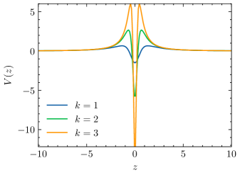
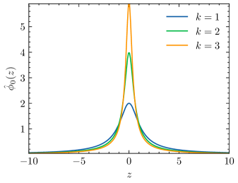
Figure 1: The plots of the effective potential and zero-mass mode with parameter $\gamma_{1}=-1$ and different values of $k$.

6 Conclusions and Discussions

The localization of $U(1)$ gauge fields in Randall-Sundrum II (RSII)-like models has been a long-standing problem in braneworld theories. To address this issue, we propose a new non-minimal coupling action inspired by the work of Germani [24]. Specifically, we modify the original action by dropping the term $\mathcal{F}_{AB}\mathcal{F}^{AB}$ and adding a new term $\gamma_{1}\mathcal{R}^{AB}_{\ \ \ CD}\mathcal{F}_{AB}\mathcal{F}^{CD}$.

With our proposed action, we are able to obtain a localized zero-mass mode, which leads to the 4D conventional $U(1)$ gauge action in 4D. Notably, our proposed action preserves gauge symmetry and avoids introducing new degrees of freedom into the scenario.

However, we also find that the massive KK modes exhibit imaginary masses, which is a feature of the action and is independent of the parameters $\gamma_{1}$ and $\gamma_{2}$.

In summary, our proposed non-minimal coupling action offers a promising solution for the localization of the $U(1)$ gauge field in braneworlds. Nevertheless, the presence of tachyonic modes warrants further investigation into the stability of the theory. It remains to be seen whether our proposed non-minimal coupling action will provide a viable solution for localizing other types of gauge fields in braneworld scenarios. In addition, while the Lagrangian (1.2) is proved to be unique in four dimensions [51], is our action (2.6) also unique in five-dimensional spacetime? We would like to address this issue in a future work.

References

- [1] L. Randall and R. Sundrum, A large mass hierarchy from a small extra dimension, Phys. Rev. Lett. 83 (1999) 3370 [hep-ph/9905221].
- [2] L. Randall and R. Sundrum, An alternative to compactification, Phys. Rev. Lett. 83 (1999) 4690 [hep-th/9906064].
- [3] M. Gremm, Four-dimensional gravity on a thick domain wall, Phys. Lett. B 478 (2000) 434 [hep-th/9912060].
- [4] B. Bajc and G. Gabadadze, Localization of matter and cosmological constant on a brane in anti de Sitter space, Phys. Lett. B 474 (2000) 282 [hep-th/9912232].
- [5] V.A. Rubakov and M.E. Shaposhnikov, Do we live inside a domain wall?, Phys. Lett. B 125 (1983) 136.
- [6] S. Randjbar-Daemi and M.E. Shaposhnikov, Fermion zero-modes on brane-worlds, Phys. Lett. B 492 (2000) 361 [hep-th/0008079].
- [7] C. Ringeval, P. Peter and J.-P. Uzan, Localization of massive fermions on the brane, Phys. Rev. D 65 (2002) 044016 [hep-th/0109194].
- [8] R. Koley and S. Kar, Scalar kinks and fermion localization in warped spacetimes, Class. Quantum Grav. 22 (2005) 753 [hep-th/0407158].
- [9] A. Melfo, N. Pantoja and J.D. Tempo, Fermion localization on thick branes, Phys. Rev. D 73 (2006) 044033 [hep-th/0601161].
- [10] Y.-X. Liu, L.-D. Zhang, L.-J. Zhang and Y.-S. Duan, Fermions on thick branes in background of Sine-Gordon kinks, Phys. Rev. D 78 (2008) 065025 [0804.4553].
- [11] Y.-X. Liu, Introduction to extra dimensions and thick braneworlds, in Memorial Volume for Yi-Shi Duan, pp. 211–275, World Scientific (2018) [1707.08541].
- [12] I. Oda, Trapping of nonAbelian gauge fields on a brane, hep-th/0103257.
- [13] B. Batell and T. Gherghetta, Yang-Mills localization in warped space, Phys. Rev. D 75 (2007) 025022 [hep-th/0611305].
- [14] K. Ohta and N. Sakai, Non-Abelian gauge field localized on walls with four-dimensional world volume, Prog. Theor. Phys. 124 (2010) 71 [1004.4078].
- [15] K. Ohta and N. Sakai, Erratum: Non-Abelian Gauge Field Localized on Walls with Four-Dimensional World Volume, Progress of Theoretical Physics 127 (2012) 1133.
- [16] M. Arai, F. Blaschke, M. Eto and N. Sakai, Matter fields and non-Abelian gauge fields localized on walls, PTEP 2013 (2013) 013B05 [1208.6219].
- [17] G. Alencar, R.R. Landim, C.R. Muniz and R.N. Costa Filho, Nonminimal couplings in Randall-Sundrum scenarios, Phys. Rev. D 92 (2015) 066006 [1502.02998].
- [18] M. Arai, F. Blaschke, M. Eto and N. Sakai, Non-Abelian gauge field localization on walls and geometric higgs mechanism, PTEP 2017 (2017) 053B01 [1703.00427].
- [19] M. Arai, F. Blaschke, M. Eto and N. Sakai, Localized non-Abelian gauge fields in non-compact extra-dimensions, PTEP 2018 (2018) 063B02 [1801.02498].
- [20] M. Arai, F. Blaschke, M. Eto, M. Kawaguchi and N. Sakai, Standard model gauge fields localized on non-Abelian vortices in six dimensions, PTEP 2021 (2021) 123B07 [2105.06026].
- [21] A. Pomarol, Gauge bosons in a five-dimensional theory with localized gravity, Phys. Lett. B 486 (2000) 153 [hep-ph/9911294].
- [22] K. Ghoroku and A. Nakamura, Massive vector trapping as a gauge boson on a brane, Phys. Rev. D 65 (2002) 084017 [hep-th/0106145].
- [23] A. Golovnev, V. Mukhanov and V. Vanchurin, Vector inflation, JCAP 0806 (2008) 009 [0802.2068].
- [24] C. Germani, Spontaneous localization on a brane via a gravitational mechanism, Phys. Rev. D 85 (2012) 055025 [1109.3718].
- [25] Z.-H. Zhao, Q.-Y. Xie and Y. Zhong, New localization method of U(1) gauge vector field on flat branes in (asymptotic) AdS5 spacetime, Class. Quantum Grav. 32 (2015) 035020 [1406.3098].
- [26] G. Alencar, R. Landim, M. Tahim and R. Costa Filho, Gauge field localization on the brane through geometrical coupling, Phys. Lett. B 739 (2014) 125 [1409.4396].
- [27] C.A. Vaquera-Araujo and O. Corradini, Localization of Abelian gauge fields on thick branes, Eur. Phys. J. C 75 (2015) 48 [1406.2892].
- [28] Z.-H. Zhao and Q.-Y. Xie, Localization of U(1) gauge vector field on flat branes with five-dimension (asymptotic) AdS5 spacetime, JHEP 2018 (2018) 72 [1712.09843].
- [29] L.F. Freitas, G. Alencar and R.R. Landim, Universal aspects of U(1) gauge field localization on branes in D-dimensions, JHEP 02 (2019) 035 [1809.07197].
- [30] T.-T. Sui, W.-D. Guo, Q.-Y. Xie and Y.-X. Liu, Generalized geometrical coupling for vector field localization on thick brane in asymptotic anti–de Sitter spacetime, Phys. Rev. D 101 (2020) 055031 [2001.02154].
- [31] R.I. de Oliveira Junior, M.O. Tahim, G. Alencar and R.R. Landim, Localization of a Model with U(1) Kinetic Gauge Mixing, Mod. Phys. Lett. A 35 (2020) 2050047.
- [32] Y. Isozumi, K. Ohashi and N. Sakai, Massless Localized Vector Field on a Wall in D=5 SQED with Tensor Multiplets, JHEP 11 (2003) 061 [hep-th/0310130].
- [33] A. Chumbes, J. Hoff da Silva and M. Hott, A model to localize gauge and tensor fields on thick branes, Phys. Rev. D 85 (2012) 085003 [1108.3821].
- [34] Z.-H. Zhao, Y.-X. Liu and Y. Zhong, U(1) gauge field localization on a Bloch brane with Chumbes-Holf da Silva-Hott mechanism, Phys. Rev. D 90 (2014) 045031 [1402.6480].
- [35] A. Kehagias and K. Tamvakis, Localized gravitons, gauge bosons and chiral fermions in smooth spaces generated by a bounce, Phys. Lett. B 504 (2001) 38 [hep-th/0010112].
- [36] T.-T. Sui and L. Zhao, Localization of vector field on pure geometrical thick brane, Chin. Phys. Lett. 34 (2017) 061101 [1703.05653].
- [37] M. Arai, F. Blaschke, M. Eto and N. Sakai, Topological massless bosons on edges: Jackiw-Rebbi mechanism for bosonic fields, Physical Review D 100 (2019) 095014 [1811.08708].
- [38] M. Eto and M. Kawaguchi, Localization of gauge bosons and the Higgs mechanism on topological solitons in higher dimensions, JHEP 10 (2019) 098 [1907.04573].
- [39] C.-E. Fu, Z.-h. Zhao and M.-H. Sun, Gauge invariance and localization of vector Kaluza–Klein modes, Eur. Phys. J. C 82 (2022) 102.
- [40] A. Prasanna, A new invariant for electromagnetic fields in curved space-time, Physics Letters A 37 (1971) 331.
- [41] H.A. Buchdahl, On a Lagrangian for non-minimally coupled gravitational and electromagnetic fields, J. Phys. A: Math. Gen. 12 (1979) 1037.
- [42] F. Mueller-Hoissen, Nonminimal coupling from dimensional reduction of the Gauss-Bonnet action, Phys. Lett. B 201 (1988) 325.
- [43] C.W. Misner, K.S. Thorne and J.A. Wheeler, Gravitation, W. H. Freeman, San Francisco (1973).
- [44] T.A. Chowdhury, R. Rahman and Z.A. Sabuj, Gravitational properties of the Proca field, Nuclear Physics B 936 (2018) 364.
- [45] G.R. Dvali, G. Gabadadze and M.A. Shifman, (Quasi)localized gauge field on a brane: Dissipating cosmic radiation to extra dimensions?, Phys. Lett. B 497 (2001) 271 [hep-th/0010071].
- [46] T. Gherghetta, TASI lectures on a holographic view of beyond the standard model physics, 1008.2570.
- [47] C.V. Sukumar, Supersymmetric quantum mechanics of one-dimensional systems, J. Phys. A 18 (1985) 2917.
- [48] D. Bazeia, C. Furtado and A.R. Gomes, Brane structure from scalar field in warped spacetime, J. Cosmol. Astropart. Phys. 0402 (2004) 002 [hep-th/0308034].
- [49] C. Bogdanos, A. Dimitriadis and K. Tamvakis, Brane models with a Ricci-coupled scalar field, Phys. Rev. D 74 (2006) 045003 [hep-th/0604182].
- [50] Y. Zhong and Y.-X. Liu, Pure geometric thick f(R)-branes: Stability and localization of gravity, Eur. Phys. J. C 76 (2016) 321 [1507.00630].
- [51] G.W. Horndeski, Conservation of charge and the einstein-maxwell field equations, J. Math. Phys. 17 (1976) 1980.
- [52] K. Peeters, Introducing Cadabra: A Symbolic computer algebra system for field theory problems, arXiv:hep-th/0701238 (2007) [hep-th/0701238].
- [53] K. Peeters, A Field-theory motivated approach to symbolic computer algebra, Comput. Phys. Commun. 176 (2007) 550 [cs/0608005].
- [54] K. Peeters, Cadabra2: Computer algebra for field theory revisited, J. Open Source Softw. 3 (2018) 1118.