MGTANet: Encoding Sequential LiDAR Points Using Long Short-Term Motion-Guided Temporal Attention for 3D Object Detection

Abstract

Most scanning LiDAR sensors generate a sequence of point clouds in real-time. While conventional 3D object detectors use a set of unordered LiDAR points acquired over a fixed time interval, recent studies have revealed that substantial performance improvement can be achieved by exploiting the spatio-temporal context present in a sequence of LiDAR point sets. In this paper, we propose a novel 3D object detection architecture, which can encode LiDAR point cloud sequences acquired by multiple successive scans. The encoding process of the point cloud sequence is performed on two different time scales. We first design a short-term motion-aware voxel encoding that captures the short-term temporal changes of point clouds driven by the motion of objects in each voxel. We also propose long-term motion-guided bird’s eye view (BEV) feature enhancement that adaptively aligns and aggregates the BEV feature maps obtained by the short-term voxel encoding by utilizing the dynamic motion context inferred from the sequence of the feature maps. The experiments conducted on the public nuScenes benchmark demonstrate that the proposed 3D object detector offers significant improvements in performance compared to the baseline methods and that it sets a state-of-the-art performance for certain 3D object detection categories. Code is available at https://github.com/HYjhkoh/MGTANet.git.

Introduction

3D object detectors detect, localize, and classify objects in a 3D coordinate system. Notably, 3D object detection is essential in various robotic and autonomous driving applications. Accordingly, to date, various LiDAR-based 3D object detectors have been proposed (Yan, Mao, and Li 2018; Lang et al. 2019; Zhou and Tuzel 2018; Deng et al. 2020; Shi, Wang, and Li 2019; Yang et al. 2020; Shi and Rajkumar 2020; Chen et al. 2019; Yang et al. 2019; Shi et al. 2020; He et al. 2020). In these works, 3D object detection was performed based on a single set of LiDAR point clouds acquired from a fixed number of laser scans. The point data in each set are unordered, and only the geometrical distributions of points are used to extract the features. In several robotics applications, LiDAR sensors stream point cloud sequences in real time through continuous scanning. However, existing 3D object detection methods do not utilize the temporal distribution of sequential LiDAR points, leaving room for improving the detection performance.

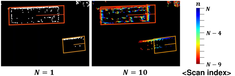
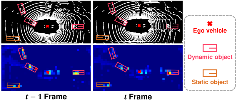
Figure 1: Visualization of (a) LiDAR points acquired over multiple scans (1 scan versus 10 scans) and (b) bird’s-eye-view (BEV) feature maps obtained from the adjacent frames.

In the literature, there exist numerous relevant studies. Similar problems have been considered in video object detection, which detects objects using multiple adjacent video frames (Feichtenhofer, Pinz, and Zisserman 2017; Zhu et al. 2017; Wang et al. 2018a; Deng et al. 2019; Wu et al. 2019; Guo et al. 2019; Kim et al. 2021; Chen et al. 2020c; Koh et al. 2021). The primary interest of these studies focused on enhancing visual features using a sequence of video frames. Recently, this study has been extended to LiDAR-based 3D object detection (Huang et al. 2020; Yin et al. 2020; Yuan et al. 2021; Emmerichs, Pinggera, and Ommer 2021; Yang et al. 2021). In this study, the 3D object detectors that consume the temporal sequence of point clouds are called 3D object detection with point cloud sequence (3D-PCS). Several 3D-PCS methods have employed various sequence encoding models to aggregate the intermediate features obtained from each set of points (Huang et al. 2020; Yin et al. 2020; Yuan et al. 2021; Emmerichs, Pinggera, and Ommer 2021; Yang et al. 2021). The method in (Huang et al. 2020) was based on a ConvLSTM model (Xingjian et al. 2015) modified to capture a temporal structure in a sequence of point features. 3DVID (Yin et al. 2020) incorporated an attentive spatio-temporal memory in a ConvGRU model (Ballas et al. 2015) to enable spatio-temporal reasoning across a long-term point cloud sequence. VelocityNet (Emmerichs, Pinggera, and Ommer 2021) used deformable convolution to generate spatio-temporal features based on the velocity patterns of dynamic objects. 3D-MAN (Yang et al. 2021) attempted proposal-level feature aggregation using a transformer architecture.

In this paper, we propose a new 3D object detector, referred to as Motion-Guided Temporal Attention Network (MGTANet), designed to encode a finite-length sequence of LiDAR point clouds. The proposed MGTANet finds a representation of sequential point sets over two different time scales.

First, $N$ sets of points acquired by successive LiDAR scans constitute a single frame and are encoded by short-term motion-guided BEV feature extraction. Figure 1 (a) illustrates the example of the point sets acquired by multiple scans. The points from different scanning grids can be observed to exhibit certain temporal patterns due to the motion of objects. These patterns can be used as contextual cues to enhance the features of objects. While most existing 3D object detectors merge these sets of points without considering their temporal context, we devise short-term motion-aware voxel feature encoding (SM-VFE) to arrange the sets of points in the scanning order and perform sequence modeling in the latent motion embedding space. The voxel features produced by the short-term voxel encoding are then transformed into bird’s-eye-view (BEV) domain features using a standard convolutional neural network (CNN) backbone.

Second, $K$ BEV feature maps obtained by the short-term voxel encoding over $K$ successive frames are aggregated through long-term motion-guided BEV feature enhancement. 3D motion of objects causes dynamic changes in BEV features over frames (see Figure 1 (b)), so these features should be aligned to boost the effect of feature aggregation. Motivated by the idea that the motion context provides a valuable clue for temporal feature alignment, we propose the motion-guided deformable alignment (MGDA) that extracts the motion features from two adjacent multi-scale BEV features and uses them to determine the position offsets and weights of the deformable masks. We also propose a novel spatio-temporal feature aggregation (STFA) that combines the aligned BEV features via spatio-temporal deformable attention. While the existing deformable DETR (Zhu et al. 2020b) cannot adaptively apply a deformable mask to each BEV feature map due to structural limitations, we introduce the concept of derivative queries to utilize the relationship with the feature map of interest in aggregating the adjacent BEV feature maps. This novel structure allows multiple BEV feature maps to be weighted and aggregated in an effective and computationally-efficient manner.

Our experiment results on a widely used public nuScenes dataset (Caesar et al. 2020) confirm that the proposed MGTANet outperforms existing 3D-PCS methods by significant margins and set a state-of-the-art performance in some evaluation metrics in the benchmark.

The key contributions of our study are summarized as follows.

• We propose a new 3D object detection architecture, MGTANet that exploits the spatio-temporal information in point cloud sequences both in short-term and long-term time scales.

• We design an enhanced voxel encoding architecture that performs sequence modeling by considering LiDAR scanning orders in a short sequence. In order to model points acquired by successive LiDAR scans in each voxel, a latent motion feature is augmented to each voxel representation. To the best of our knowledge, voxel encoding that accounts for temporal point distribution has not been introduced in the previous literature.

• We present a long-term feature aggregation method to find the representation of multiple BEV feature maps that dynamically vary over longer time scales. Our evaluation shows that motion context information extracted from the adjacent BEV feature maps plays a pivotal role in finding better representation of the sequential feature maps. Combination of both short-term and long-term encoding of LiDAR point cloud sequences offers performance gains up to 5.1 % in mean average prediction (mAP) and 3.9 % in nuScenes detection score (NDS) over CenterPoint baseline (Yin, Zhou, and Krahenbuhl 2021) on the nuScenes 3D object detection benchmark.

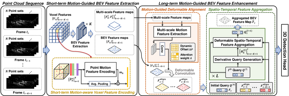
Figure 2: Overall architecture of the proposed MGTANet. MGTANet comprises three main blocks. SM-VFE performs voxel encoding based on a LiDAR point cloud sequence acquired over multiple LiDAR scans in a short sequence. MGDA then aligns the previous BEV feature maps to the current BEV feature map. Finally, STFA aggregates only the relevant parts of the aligned feature maps using a deformable cross-attention mechanism.

Related Work

3D Object Detection with a Single Point Set

LiDAR-based 3D object detectors can be roughly categorized into grid encoding-based methods (Yan, Mao, and Li 2018; Zhou and Tuzel 2018; Lang et al. 2019; Deng et al. 2020), point encoding-based methods (Shi, Wang, and Li 2019; Yang et al. 2020; Shi and Rajkumar 2020), and hybrid methods (Chen et al. 2019; Yang et al. 2019; Shi et al. 2020; He et al. 2020). Among these, grid encoding-based methods organize the irregular point clouds using regular grid structures such as voxels (Zhou and Tuzel 2018) or pillars (Lang et al. 2019) and extract the volumetric representations. In contrast, point encoding-based methods retain geometrical information of point clouds and extract point-wise features using PointNet (Qi et al. 2017a) or PointNet++ (Qi et al. 2017b). Moreover, some approaches take advantage of the merits of both these methods. In our study, the grid encoding-based methods are adopted as a baseline detector since they are more prevalent in training large-scale datasets such as nuScenes with state-of-the-art detection performance.

3D Object Detection with Point Cloud Sequence

The performance of 3D object detection methods can be improved by exploiting the temporal information in the LiDAR point cloud sequences. To date, several 3D-PCS methods have been proposed (Huang et al. 2020; Yin et al. 2020; Yuan et al. 2021; Emmerichs, Pinggera, and Ommer 2021; Yang et al. 2021). These methods explored various ways to find the representation of time-varying features obtained from multiple point sets. The method proposed in (Huang et al. 2020) encoded temporal LiDAR features using long short term memory (LSTM) and 3DVID (Yin et al. 2020) realized an improved sequence modeling ability using an attentive spatio-temporal Transformer GRU. TCTR (Yuan et al. 2021) modeled temporal-channel information of multiple frames and decoded spatial-wise information using a transformer architecture. VelocityNet (Emmerichs, Pinggera, and Ommer 2021) aligned temporal feature maps using deformable convolution driven by a motion map obtained from the velocities of objects. 3D-MAN (Yang et al. 2021) stored the proposals and features obtained from a fast single-frame detector in a memory bank and fused them using a multi-view alignment and aggregation module.

The proposed MGTANet differs from the aforementioned methods in that it presents a holistic approach to process the temporal information of the point cloud sequences. Within point sets that exhibit only slight motion on a short-term scale, the proposed method captures the temporal distribution of points through voxel encoding. The proposed approach also considers the novel motion-guided feature alignment approach to actively adapt to dynamic feature changes occuring over longer time scales.

Proposed Method

In this section, we present the details of the proposed 3D object detector based on point cloud sequences.

Overview

The overall architecture of the proposed MGTANet is depicted in Figure 2. The proposed 3D-PCS method consists of three main blocks; 1) short-term motion-aware voxel feature encoding (SM-VFE) 2) motion-guided deformable alignment (MGDA), and 3) spatio-temporal feature aggregation (STFA). Herein, SM-VFE is performed in a short sequence to encode enhanced voxel representations, whereas both MGDA and STFA are performed in long sequences to extract spatio-temporal BEV features under the guidance of motion information.

We assume that a LiDAR sensor generates a sequence of point clouds as it scans. The point clouds $P_{k}^{n}$ denote the point set acquired from the $n$th scanning step and the $k$th frame. The $k$th frame consists of $N$ consecutive point sets, i.e., $I_{k}=\{P_{k}^{n}\}_{n=1}^{N}$. The ego-motion compensation is applied to the point sets within each frame (Caesar et al. 2020). MGTANet uses a total of $N\times K$ point sets in the latest $K$ frames $\{I_{k}\}_{k=t-K+1}^{t}$ as inputs and produces the object detection results for the $t$th frame, where $t$ denotes the index for the frame of interest.

The $N$ point sets in each frame are encoded using the SM-VFE. First, these $N$ point sets are voxelized by a pre-defined grid size. Each voxel contains the points that belong to different point sets $P_{k}^{1},P_{k}^{2},...,P_{k}^{N}$ and exhibits a particular motion pattern over $N$ point sets. The proposed SM-VFE extracts a voxel embedding vector that models the temporal distribution of such points obtained from each voxel. The voxel features $\{\textbf{{V}}_{k}\}_{k=t-K+1}^{t}$ generated by SM-VFE are further encoded by a sparse 3D CNN backbone to produce the $K$ BEV feature maps $\{\textbf{{F}}_{k}\}_{k=t-K+1}^{t}$ (Yan, Mao, and Li 2018).

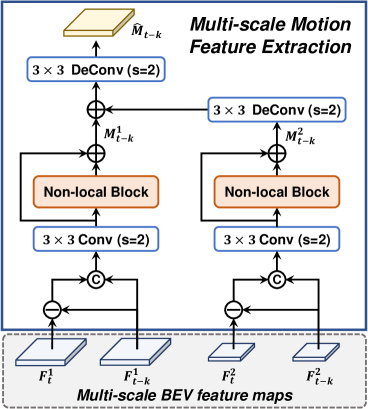
(a) Multi-scale motion feature extraction

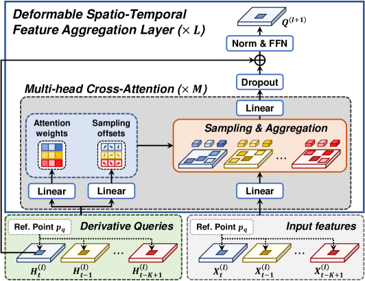
(b) Deformable spatio-temporal feature aggregation

Figure 3: Structure of sub-modules in long-term motion-guided BEV feature enhancement model (a) Multi-scale motion feature extraction module extracts the motion context feature with multi-scale BEV features. (b) Deformable spatio-temporal feature aggregation module implements multi-head cross-attention to aggregate the adjacent BEV feature maps.

Next, the BEV feature maps $\{\textbf{{F}}_{k}\}_{k=t-K+1}^{t}$ are aggregated over a longer time scale. Before these features are aggregated, they are spatially aligned to improve the effect of feature aggregation. First, MGDA aligns the previous $K-1$ BEV feature maps $\{\textbf{{F}}_{k}\}_{k=t-K+1}^{t-1}$ to the current BEV feature map $\textbf{{F}}_{t}$ under the guidance of contextual motion information. MGDA performs deformable convolution (Dai et al. 2017) to align each BEV feature map. The motion features extracted from multi-scale BEV feature maps are used to determine the sampling offsets and attention weights of the deformable masks. MGDA produces the aligned BEV features $\textbf{{F}}_{t-1}^{align},...,\textbf{{F}}_{t-K+1}^{align}$. Then, STFA aggregates the $K$ BEV feature maps $\textbf{{F}}_{t},\textbf{{F}}_{t-1}^{align},...,\textbf{{F}}_{t-K+1}^{align}$ using the deformable cross-attention model modified to enable spatio-temporal attention. Finally, STFA produces the aggregated feature map, $\hat{\textbf{{F}}}_{t}$, which is further processed by the 3D detection head to output the final 3D detection results.

Short-term Motion-aware Voxel Feature Encoding

SM-VFE encodes LiDAR points considering the geometrical change occurring over time in each voxel. First, the $N$ point sets $\{P_{k}^{n}\}_{n=1}^{N}$ in the $k$th frame are merged and voxelized using a voxel structure (Zhou and Tuzel 2018) or a pillar structure (Lang et al. 2019). Then, each voxel contains the $N$ point sets $\{\tilde{P}_{k}^{n}\}_{n=1}^{N}$ sub-sampled from $\{P_{k}^{n}\}_{n=1}^{N}$. Let the cardinality of $\tilde{P}_{k}^{n}$ be $N_{k}^{n}$ and the $i$th element of $\tilde{P}_{k}^{n}$ be $\tilde{p}_{k}^{n}(i)$. The point entity $\tilde{p}_{k}^{n}(i)$ contains the $(x,y,z)$ 3D coordinates, reflectance, and time lag of a LiDAR point. We perform averaging operation over the elements of each point set $\tilde{P}_{k}^{n}$ as

$$\bar{p}_{k}^{n}=\frac{1}{N_{k}^{n}}\sum_{i=1}^{N_{k}^{n}}\tilde{p}_{k}^{n}(i).$$ (1)

If $\tilde{P}_{k}^{n}$ is empty, $\bar{p}_{k}^{n}$ is set to a zero vector of the same length. Next, we encode the sequence of $N$ points $\{\bar{p}_{k}^{n}\}_{n=1}^{N}$. For this, differential encoding is applied to represent the motion with respect to the last point $\bar{p}_{k}^{N}$, i.e., $D_{k}=\{\bar{p}_{k}^{N}-\bar{p}_{k}^{n}\}_{n=1}^{N-1}$. Each motion vector $(\bar{p}_{k}^{N}-\bar{p}_{k}^{n})$ passes through the fully-connected ($\mathrm{FC}$) layer, which is followed by the channel-wise attention ($\mathrm{CWA}$) (Hu, Shen, and Sun 2018), as given below

$$q_{k}^{n}=\mathrm{CWA}(\mathrm{FC}(\bar{p}_{k}^{N}-\bar{p}_{k}^{n})).$$ (2)

Finally, the sequence $\{q_{k}^{n}\}_{n=1}^{N-1}$ is concatenated and encoded by an additional $\mathrm{FC}$ layer

$$m_{k}=\mathrm{FC}(\mathrm{Concat}(\{q_{k}^{n}\}_{n=1}^{N-1})).$$ (3)

This motion feature $m_{k}$ is concatenated to the original voxel features computed by VoxelNet (Zhou and Tuzel 2018) or PointPillars (Lang et al. 2019). These motion-aware voxel features are delivered to a conventional sparse 3D CNN backbone for further encoding (Yan, Mao, and Li 2018).

Motion-Guided Deformable Alignment

MGDA aligns the adjacent BEV feature maps $\{\textbf{{F}}_{k}\}_{k=t-K+1}^{t}$ using motion-guided deformable convolution. For feature alignment, MGDA applies a deformable convolution (Zhu et al. 2019b) to each of the previous feature maps $\{\textbf{{F}}_{k}\}_{k=t-K+1}^{t-1}$. The deformable mask applied to $\textbf{{F}}_{t-k}$ is determined by the motion features computed based on the following two features $\textbf{{F}}_{t-k}$ and $\textbf{{F}}_{t}$.

Figure 3 (a) presents the structure of the motion feature extraction block. To extract the motion features, we consider the multi-scale features $\textbf{{F}}_{t-k}^{1},\cdots,\textbf{{F}}_{t-k}^{S}$ obtained from the intermediate layers of the network branch for producing $\textbf{{F}}_{t-k}$. Similarly, the multi-scale features $\textbf{{F}}_{t}^{1},\cdots,\textbf{{F}}_{t}^{S}$ can be obtained from the intermediate layers for $\textbf{{F}}_{t}$. These multi-scale features aid in representing motion at different scales and granularities. We only consider two scales $S=2$ in our implementation. For each scale, the motion features are obtained from

$$\tilde{\textbf{{M}}}^{s}_{t-k} =\mathrm{Conv}_{3\times 3}([\textbf{{F}}^{s}_{t-k},(\textbf{{F}}^{s}_{t}-\textbf{{F}}^{s}_{t-k})])$$ (4)

$$\textbf{{M}}^{s}_{t-k} =\tilde{\textbf{{M}}}^{s}_{t-k}+\mathrm{NLblock}(\tilde{\textbf{{M}}}^{s}_{t-k}),$$ (5)

where $s\in\{1,2\}$ denotes the scale index, $[\cdot,\cdot]$ denotes the channel-wise concatenation, and $\mathrm{NLblock}$ denotes the non-local block (Wang et al. 2018b). The features $\textbf{{M}}^{1}_{t-k}$ and $\textbf{{M}}^{2}_{t-k}$ with two different scales are resized to the same size via up-sampling. Then, they are summed element-wise to produce the final motion feature $\hat{\textbf{{M}}}_{t-k}$. Note that $\hat{\textbf{{M}}}_{t-k}$ has the same size as $\textbf{{F}}_{t-k}$.

Let $\Delta\textbf{{P}}_{t-k}$ and $\textbf{{A}}_{t-k}$ be the offsets and weights of the deformable mask applied to the features $\textbf{{F}}_{t-k}$. Note that $\Delta\textbf{{P}}_{t-k}$ and $\textbf{{A}}_{t-k}$ are simply obtained by applying a $1\times 1$ convolution to the motion feature $\hat{\textbf{{M}}}_{t-k}$. Then, the deformable mask with the offsets $\Delta\textbf{{P}}_{t-k}$ and weights $\textbf{{A}}_{t-k}$ is applied to $\textbf{{F}}_{t-k}$ for feature alignment. Finally, this operation produces the aligned BEV feature maps $\{\textbf{{F}}_{k}^{align}\}_{k=t-K+1}^{t-1}$.

Spatio-Temporal Feature Aggregation

STFA produces an enhanced feature map $\hat{\textbf{{F}}}_{t}$ by aggregating the BEV feature maps $\textbf{{F}}_{t-K+1}^{align},...,\textbf{{F}}_{t-1}^{align},\textbf{{F}}_{t}$. We re-design a deformable attention (Zhu et al. 2020b) to aggregate multi-frame features with spatio-temporal attention.

STFA successively decodes the query $\textbf{{Q}}^{(l)}$ over $L$ attention layers, where $l$ denotes the decoding layer index. In the first decoding layer, $\textbf{{Q}}^{(0)}$ is initialized by $\textbf{{F}}_{t}$. STFA performs simultaneous deformable attention on the $K$ input features $\{\textbf{{X}}_{k}^{(l)}\}_{k=t-K+1}^{t}$ denoted as

$$\textbf{{X}}_{t-k}^{(l)}=\left\{\begin{array}[]{ccc}\textbf{{F}}_{t-k}^{align}&\mbox{for}\quad k\neq 0\\ \textbf{{Q}}^{(l)}&\mbox{for}\quad k=0\end{array}\right..$$ (8)

using $K$ derivative queries $\{\textbf{{H}}_{k}^{(l)}\}_{k=t-K+1}^{t}$. The derivative query $\textbf{{H}}_{t-k}^{(l)}$ is derived from the main query $\textbf{{Q}}^{(l)}$ as

$$\textbf{{H}}_{t-k}^{(l)}=\left\{\begin{array}[]{ccc}\mathrm{Conv}_{3\times 3}([\textbf{{F}}_{t-k}^{align},\textbf{{Q}}^{(l)}])&\mbox{for}\quad k\neq 0\\ \textbf{{Q}}^{(l)}&\mbox{for}\quad k=0\end{array}\right..$$ (11)

The derivative query $\textbf{{H}}_{t-k}^{(l)}$ is used to determine the offsets and weights of the deformable masks applied to $\textbf{{X}}_{t-k}^{(l)}$. When $k\neq 0$, the derivative query $\textbf{{H}}_{t-k}^{(l)}$ depends on both $\textbf{{F}}_{t-k}^{align}$ and $\textbf{{Q}}^{(l)}$, since the deformable mask for $\textbf{{F}}_{t-k}^{align}$ should be determined based on the information present in both the $(t-k)$th and the $t$th frames. In contrast, when $k=0$, the derivative query $\textbf{{H}}_{t}^{(l)}$ is determined solely by $\textbf{{Q}}^{(l)}$.

Figure 3 (b) depicts the deformable attention with $M$ multi-heads using the derivative queries $\{\textbf{{H}}_{k}^{(l)}\}_{k=t-K+1}^{t}$. Let $q$ index $HW$ elements of the input feature map, where $W$ and $H$ denote the width and height of input features. Consider a 2D reference point $p_{q}$ at the location of $q$th element of the input feature map. Given the mask offset $\Delta_{t-k,qmj}^{(l)}$ and attention weight $A_{t-k,qmj}^{(l)}$, the feature aggregation is performed as

$$y_{q}= \sum_{m=1}^{M}W_{m}(\sum_{k=0}^{K-1}\sum_{j=1}^{J}A_{t-k,qmj}^{(l)}W_{m}^{{}^{\prime}}$$

$$\cdot\textbf{{X}}_{t-k}^{(l)}(p_{q}+\Delta_{t-k,qmj}^{(l)})),$$ (12)

where $m$ and $j$ are the multi-head index and sampling point index, respectively. $W_{m}\in\mathbb{R}^{C\times(C/M)}$ and $W_{m}^{{}^{\prime}}\in\mathbb{R}^{(C/M)\times(C)}$ denote the learnable projection matrices, where $C$ is the channel size of the input feature. We let $\textbf{{X}}_{t-k}^{(l)}(p)$ be the element of $\textbf{{X}}_{t-k}^{(l)}$ at the position $p$. The mask offsets $\Delta_{t-k,qm}^{(l)}$ and the attention weights $A_{t-k,qm}^{(l)}$ are obtained from

$$\Delta_{t-k,qm}^{(l)} =W_{\Delta,m}(\textbf{{H}}_{t-k}^{(l)}(p_{q}))$$ (13)

$$A_{t-k,qm}^{(l)} =\mathrm{Softmax}(W_{A,m}(\textbf{{H}}_{t-k}^{(l)}(p_{q}))),$$ (14)

where $\Delta_{t-k,qm}^{(l)}=\left[\Delta_{t-k,qm1}^{(l)},\cdots,\Delta_{t-k,qmJ}^{(l)}\right]^{T}$, and $A_{t-k,qm}^{(l)}=\left[A_{t-k,qm1}^{(l)},\cdots,A_{t-k,qmJ}^{(l)}\right]^{T}$, $\mathrm{Softmax(\cdot)}$ is the softmax function, and $W_{\Delta,m}(\in\mathbb{R}^{2J\times C})$ and $W_{A,m}(\in\mathbb{R}^{J\times C})$ are the learnable projection matrices.

Finally, the $q$th element of main query is updated as

$$\textbf{{Q}}^{(l+1)}(p_{q})=\mathrm{FFN}(\mathrm{LN}(\mathrm{Dropout}(y_{q})+\textbf{{Q}}^{(l)}(p_{q}))),$$ (15)

where $\mathrm{FFN}(\cdot)$ denotes feed-forward network (Vaswani et al. 2017), $\mathrm{LN(\cdot)}$ denotes the layer normalization (Ba, Kiros, and Hinton 2016), and $\mathrm{Dropout(\cdot)}$ denotes the drop-out operation (Srivastava et al. 2014). After $L$ layers of query decoding, the aggregated BEV feature maps can finally be obtained as $\hat{\textbf{{F}}}_{t}=\textbf{{Q}}^{(L)}$.

  Method NDS mAP Car Truck Bus Trailer C.V Ped. Motor. Bicycle T.C Barrier PointPillars (Lang et al. 2019) 45.3 30.5 68.4 23.0 28.2 23.4 4.1 59.7 27.4 1.1 30.8 38.9 WYSIWYG (Hu et al. 2020) 41.9 35.0 79.1 30.4 46.6 40.1 7.1 65.0 18.2 0.1 28.8 34.7 3DSSD (Yang et al. 2020) 56.4 42.6 81.2 47.2 61.4 30.5 12.6 7.2 36.0 8.6 31.1 47.9 SA-Det3D (Bhattacharyya, Huang, and Czarnecki 2021) 59.2 47.0 81.2 43.8 57.2 47.8 11.3 73.3 32.1 7.9 60.6 55.3 SSN V2 (Zhu et al. 2020a) 61.6 50.6 82.4 41.8 46.1 48.0 17.5 75.6 48.9 24.6 60.1 61.2 CBGS (Zhu et al. 2019a) 63.3 52.8 81.1 48.5 54.9 42.9 10.5 80.1 51.5 22.3 70.9 65.7 CVCNet (Chen et al. 2020a) 64.2 55.8 82.7 46.1 45.8 46.7 20.7 81.0 61.3 34.3 69.7 69.9 HotSpotNet (Chen et al. 2020b) 66.6 59.3 83.1 50.9 56.4 53.3 23.0 81.3 63.5 36.6 73.0 71.6 CyliNet (Rapoport-Lavie and Raviv 2021) 66.1 58.5 85.0 50.2 56.9 52.6 19.1 84.3 58.6 29.8 79.1 69.0 CenterPoint (Yin, Zhou, and Krahenbuhl 2021) 67.3 60.3 85.2 53.5 63.6 56.0 20.0 84.6 59.5 30.7 78.4 71.1 AFDetV2 (Hu et al. 2022) 68.5 62.4 86.3 54.2 62.5 58.9 26.7 85.8 63.8 34.3 80.1 71.0 S2M2-SSD (Zheng et al. 2022) 69.3 62.9 86.3 56.0 65.4 59.8 26.2 84.5 61.6 36.4 77.7 75.1 TransFusion-L (Bai et al. 2022) 70.2 65.5 86.2 56.7 66.3 58.8 28.2 86.1 68.3 44.2 82.0 78.2 VISTA (Deng et al. 2022) 70.4 63.7 84.7 54.2 64.0 55.0 29.1 83.6 71.0 45.2 78.6 71.8 3DVID (with PointPillars) (Yin et al. 2020) 53.1 45.4 79.7 33.6 47.1 43.1 18.1 76.5 40.7 7.9 58.8 48.8 3DVID (with CenterPoint) (Yin et al. 2021) 71.4 65.4 87.5 56.9 63.5 60.2 32.1 82.1 74.6 45.9 78.8 69.3 MGTANet-P 61.4 50.9 81.3 45.8 55.0 48.9 18.2 74.4 52.6 17.8 61.7 53.0 MGTANet-C 71.2 65.4 87.7 56.9 64.6 59.0 28.5 86.4 72.7 47.9 83.8 65.9 MGTANet-CT 72.7 67.5 88.5 59.8 67.2 61.5 30.6 87.3 75.8 52.5 85.5 66.3  

Table 1: Performance on nuScenes test benchmark. The model is trained on nuScenes train set and evaluated on nuScenes test set. C.V and T.C, respectively, indicates the construction vehicle and the traffic cone. Ped. and Motor. are short for the motorcycle and the pedestrian, respectively. The best performance are in boldface.

Experiments

nuScenes dataset

The nuScenes dataset (Caesar et al. 2020) is a large-scale autonomous driving dataset that contains 700, 150, and 150 scenes for training, validation, and testing. It comprises LiDAR point cloud data acquired at 20Hz using 32-channel LiDAR. Keyframe samples are provided at 2Hz with 360-degree object annotations. The dataset also provides intermediate sensor frames. Average precision (AP) metric defines a match by thresholding the 2D center distance on the ground plane, and NDS metric is the one suggested by nuScenes 3D object detection benchmark (Caesar et al. 2020). These metrics were used to evaluate the performance of our proposed 3D detection method on 10 object categories (barrier, bicycle, bus, car, motorcycle, pedestrian, trailer, truck, construction vehicle, and traffic cone).

Implementation details

Data Processing. Following the format of nuScenes dataset (Caesar et al. 2020), a single frame consists of $N=10$ multiple LiDAR scans, i.e., 10 point sets. Each LiDAR point is represented as $(x,y,z,r,\Delta t)$, where $(x,y,z)$ denotes the coordinate of a 3D point, $r$ denotes the reflectance, and $\Delta t$ denotes the time delta in seconds from the keyframe. In our experiment, the number of frames $K$ processed by the MGTANet was set to 3, corresponding to a duration of 1.5 seconds.

Network Architecture. The proposed method was implemented on two widely used 3D object detectors, PointPillars (Lang et al. 2019) and CenterPoint (Yin, Zhou, and Krahenbuhl 2021). For PointPillars, the range of point clouds was within $[-51.2,51.2]\times[-51.2,51.2]\times[-5.0,3.0]m$ on the $(x,y,z)$ axes and the LiDAR voxel structure comprised $512\times 512\times 1$ voxel grids with a grid size of $0.2\times 0.2\times 8.0m$. We chose the CenterPoint (Yin, Zhou, and Krahenbuhl 2021) using the backbone used in SECOND (Yan, Mao, and Li 2018). The voxelization range was set to $[-54.0,54.0]\times[-54.0,54.0]\times[-5.0,3.0]m$ along the $(x,y,z)$ axes. The size of a voxel was set to $(0.075\times 0.075\times 0.2m)$, and the dimension of the voxel structure was set to $1440\times 1440\times 40$. In our evaluation, we considered three versions of MGTANet, including 1) MGTANet-P: MGTANet with a PointPillars baseline, 2) MGTANet-C: MGTANet with a CenterPoint baseline, and 3) MGTANet-CT: MGTANet with a CenterPoint baseline and with test time augmentation (Shanmugam et al. 2021) enabled. Following the configuration of the 3DVID method (Yin et al. 2021), MGTANet-C and MGTANet-CT were implemented to allow a latency by one frame.

Training. Our model was trained in two stages. In the first stage, we trained the SM-VFE, backbone, and detection head jointly in the same manner as single-frame 3D detectors. A one-cycle learning rate policy was used for 20 epochs with a maximum learning rate of 0.001. After initializing the model with the weights obtained from the first training stage, our entire network was fine-tuned for 40 epochs with the same learning rate scheduling policy but with a maximum learning rate of 0.0002. The Adam optimizer was used to optimize the network in both stages. We utilized the loss function used in (Lang et al. 2019) and (Yin, Zhou, and Krahenbuhl 2021). We applied data augmentation methods during pre-training and fine-tuning, including random flipping, rotation, scaling, and ground-truth box sampling (Yan, Mao, and Li 2018). The batch size was set to 16 for MGTANet-P and 8 for MGTANet-C and MGTANet-CT.

  Method Proposed 3D-PCS Strategy Performance Short-term Motion-aware VFE Spatio-Temporal Feature Aggregation Motion-Guided Deformable Alignment mAP (%) NDS (%) Baseline 54.99 63.33 Our MGTANet ✓ 56.52_↑1.53 64.22_↑0.89 ✓ ✓ 58.24_↑3.25 65.22_↑1.89 ✓ ✓ ✓ 59.61_↑4.62 65.94_↑2.61  

Table 2: Ablation study on the nuScenes valid set. The effects of three main modules are highlighted in this study.

  Method Performance mAP (%) NDS (%) Baseline 54.99 63.33 + Motion embedding 56.24_↑1.25 64.00_↑0.67 + Channel-wise attention 56.52_↑1.53 64.22_↑0.89  

Table 3: Ablation study to evaluate the sub-modules of SM-VFE.

Performance on nuScenes test set.

Table 1 provides the performance of several LiDAR-based 3D object detectors evaluated on nuScenes 3D object detection tasks. The results for other LiDAR-based methods are brought from the nuScenes leaderboard except for 3DVID. Note that MGTANet-CT outperforms other latest 3D object detectors in the leaderboard. To the best of our knowledge, 3DVID (Yin et al. 2020, 2021) had the record of state-of-the-art (SOTA) performance among the existing methods based on point cloud sequences. MGTANet-CT surpassed 3DVID, setting a new SOTA performance. Note that MGTANet-P achieved an 8.3% better performance in NDS compared to the 3DVID with PointPillars baseline (Yin et al. 2020). The performance of MGTANet-C is comparable to that of 3DVID with a CenterPoint baseline (Yin et al. 2021); however, MGTANet-CT demonstrates better performance.

By encoding point cloud sequences, MGTANet exhibited a remarkable improvement in performance compared to the baseline methods. MGTANet-P achieved 16.1% gain in NDS and 20.4% gain in mAP over PointPillars baseline. MGTANet-C achieved up to 3.9% gain in NDS and 5.1% gain in mAP over CenterPoint baseline. This demonstrates that the spatio-temporal context information contained in a point cloud sequence can significantly contribute to improving the performance of 3D object detection method.

Ablation studies on nuScenes valid set

We conducted several ablation studies on the nuScenes validation set. To reduce the time required for these experiments, we used only 1/7 of the training set to perform training and the entire validation set for evaluation. We used CenterPoint (Yin, Zhou, and Krahenbuhl 2021) as a baseline detector for all ablation studies.

Three main modules. Table 2 shows the contributions of SM-VFE, MGDA, and STFA to the overall performance. Using spatio-temporal information in the voxel encoding stage, SM-VFE improves the performance of the baseline by 1.53% in mAP. When both SM-VFE and STFA are enabled, i.e., the multiple BEV features encoded using SM-VFE are aggregated by STFA without feature alignment, the mAP performance is improved by additional 1.72%. Finally, when we add MGDA module to boost the effect of feature aggregation, 1.37% further mAP improvement is achieved. Combination of all three modules offers a total performance gain of 4.62% in mAP and 2.61% in NDS over the CenterPoint baseline.

Sub-modules of SM-VFE. Table 3 provides the performance achieved by each component of SM-VFE. We use the vanilla voxel encoding method of CenterPoint as a baseline. When we add the motion embedding to the voxel features, the mAP is improved by 1.25% over the baseline. The channel-wise attention strategy yields additional gains of 0.28% in mAP and 0.22% in NDS by weighting the motion-sensitive channels of the latent features.

Derivative query for STFA. Table 4 demonstrates the effectiveness of the derivative queries used in STFA. Baseline* indicates the method that adds SM-VFE voxel encoding method to CenterPoint. Single query indicates the method that determines the deformable masks only using the main query features. Note that the derivative queries offer a performance gain of 0.74% in mAP and 0.38% in NDS over the single query. This shows that the derivative queries effectively leverage the capabilities of our spatio-temporal cross-attention mechanism.

  Method Query type Performance mAP (%) NDS (%) Baseline* - 56.52 64.22 STFA Single 57.50_↑0.98 64.84_↑0.62 Derivative 58.24_↑1.72 65.22_↑1.00  

Table 4: Comparison of derivative queries versus a single query in STFA.

Conclusions

In this paper, we proposed a new 3D object detection method MGTANet designed to model temporal structures in point cloud sequences. The proposed MGTANet can effectively find the spatio-temporal representation of point cloud sequences using motion context. First, we proposed the enhanced voxel encoding method, SM-VFE to model the temporal distribution of points acquired from consecutive LiDAR scans. We devised the latent motion embedding method that can enhance the quality of the voxel features. Second, we proposed the architecture for aggregating the BEV feature maps produced by the SM-VFE over multiple frames. First, MGDA aligned the adjacent BEV feature maps through the deformable convolution. The offsets and weights of the deformable masks were determined based on multi-scale motion features. STFA then aggregated the multiple BEV feature maps aligned by MGDA using spatio-temporal deformable attention. We introduced the derivative queries, which can enable simultaneous co-attention to the adjacent BEV features. Our evaluation conducted on nuScenes dataset confirmed that the proposed MGTANet exhibited significant improvements in performance compared to LiDAR-only baselines; moreover it outperformed the latest top-ranked 3D-PCS methods on the nuScenes 3D object detection leaderboard.

Appendix

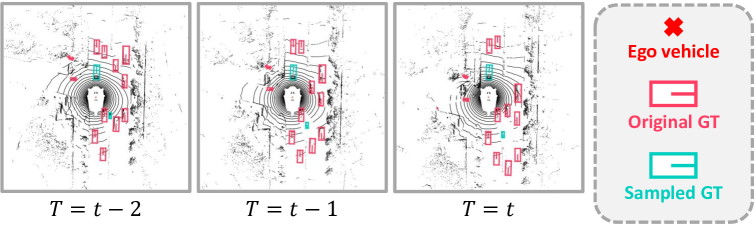
Figure 1: Visualization of GT sampling. We implement GT sampling by keeping relative motion of objects within sequence.

Implementation Details of Data Augmentations

In training stage, we apply the data augmentations, including random flipping, global scaling, global rotation, and GT sampling(Yan, Mao, and Li 2018). We randomly flipped the LiDAR points, and rotated the point cloud within a range of $[-\frac{\pi}{4},\frac{\pi}{4}]$ along the $z$ axis. We also scaled the coordinates of the points with a factor within $[0.95.1.05]$. As used in (Yan, Mao, and Li 2018), we randomly sampled several ground truth 3D boxes from other scenes and pasted corresponding 3D objects as a point cloud into the frame of interest. To leverage the capabilities of temporal information, this augmentation was applied to the neighboring frame while maintaining the relative motion pattern within sequence as depicted in Figure 1. In the last 5 epochs in training stage, we apply these augmentation techniques except GT sampling to point cloud sequences by consistently using random parameters.

Additional Experiments

Effectiveness of MGDA. Table 1 shows the effectiveness of MGDA. To simplify these experiments, BEV features are aggregated by the simple method, where the BEV features from multiple frames are concatenated, and fed into a $3\times 3$ convolution layer. When this simple strategy is applied to the CenterPoint without MGDA, the performance is reduced by 2.36% in mAP and by 1.80% in NDS. In contrast, we observe that MGDA improves the performance by 3.38% in mAP and by 2.26% in NDS over baseline. This demonstrates that feature alignment is considered crucial for performing feature aggregation.

  Method Performance mAP (%) NDS (%) Baseline 54.99 63.33 w/o MGDA 52.63 ($\downarrow 2.36$) 61.53 ($\downarrow 1.80$) with MGDA 58.37 ($\uparrow 3.38$) 65.59 ($\uparrow 2.26$)  

Table 1: Ablation study for effectiveness of MGDA.

Performance comparison on nuScenes valid set Table 2 compares our MGTANet with several LiDAR-based 3D object detectors on the nuScenes(Caesar et al. 2020). We used the whole training set for training and the whole validation set for evaluating. Our framework works in both online and offline modes. The MGTANet-C with online mode employs two previous frames to produce detection results in the frame of interest, and achieves 3.3% performance gain in mAP and 1.9% performance gain in NDS over our baseline. When applying offline mode using a previous frame and a current frame, our model achieves the best results with 64.8% mAP and 70.6% NDS.

  Method NDS mAP Car Truck Bus Trailer C.V Ped. Motor. Bicycle T.C Barrier CBGS (Zhu et al. 2019a) 56.3 56.3 82.9 52.9 64.7 37.5 18.3 80.3 60.1 39.4 64.8 64.3 CVCNet (Chen et al. 2020a) 65.5 54.6 83.2 50.0 62.0 34.5 20.2 81.2 54.4 33.9 61.1 65.5 HotSpotNet (Chen et al. 2020b) 66.0 59.5 84.0 56.2 67.4 38.0 20.7 82.6 66.2 49.7 65.8 64.3 CenterPoint* (Yin, Zhou, and Krahenbuhl 2021) 66.8 59.6 85.5 58.6 71.5 37.3 17.1 85.1 58.9 43.4 69.7 68.5 MGTANet-C* (Online-mode) 68.7 62.9 87.0 59.6 72.3 40.1 21.5 86.3 69.3 51.4 73.4 67.8 MGTANet-C* (Offline-mode) 70.6 64.8 87.9 61.3 73.2 40.2 23.0 86.6 74.1 59.9 75.7 66.1  

Table 2: Performance on nuScenes valid set. The model is trained on nuScenes whole train set and evaluated on nuScenes val set. * denotes the model implemented in the released code of CenterPoint(Yin, Zhou, and Krahenbuhl 2021).

Qualitative Results. Figure 2 and 3 shows the qualitative results of our MGTANet and CenterPoint. Our model can produce more accurate 3D detection results with fewer false positives than CenterPoint. In Figure 2, CenterPoint fails to detect far distant objects whose point clouds are sparse. In contrast, MGTANet accurately recognize these objects thanks to the temporal information from adjacent frames. Similarly, when partial occlusion occurs, as shown in Figure 3, MGTANet detects objects more accurately than CenterPoint.

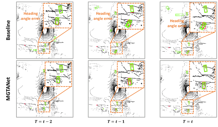
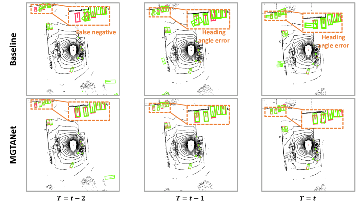
Figure 2: Comparing of CenterPoint and our MGTANet. Predicted and ground truth 3D bounding boxes are assigned with green and red, respectively. It can be found that our method shows much better results when objects are too far.

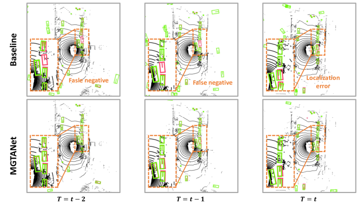
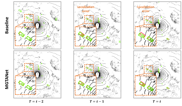
Figure 3: Comparing of CenterPoint and our MGTANet. Predicted and ground truth 3D bounding boxes are assigned with green and red, respectively. It can be found that our method shows much better results when objects are occluded by the others.

References

- Ba, Kiros, and Hinton (2016) Ba, J. L.; Kiros, J. R.; and Hinton, G. E. 2016. Layer normalization. arXiv preprint arXiv:1607.06450.
- Bai et al. (2022) Bai, X.; Hu, Z.; Zhu, X.; Huang, Q.; Chen, Y.; Fu, H.; and Tai, C.-L. 2022. Transfusion: Robust lidar-camera fusion for 3d object detection with transformers. In Proceedings of the IEEE/CVF Conference on Computer Vision and Pattern Recognition, 1090–1099.
- Ballas et al. (2015) Ballas, N.; Yao, L.; Pal, C.; and Courville, A. 2015. Delving deeper into convolutional networks for learning video representations. arXiv preprint arXiv:1511.06432.
- Bhattacharyya, Huang, and Czarnecki (2021) Bhattacharyya, P.; Huang, C.; and Czarnecki, K. 2021. Sa-det3d: Self-attention based context-aware 3d object detection. In Proceedings of the IEEE/CVF International Conference on Computer Vision, 3022–3031.
- Caesar et al. (2020) Caesar, H.; Bankiti, V.; Lang, A. H.; Vora, S.; Liong, V. E.; Xu, Q.; Krishnan, A.; Pan, Y.; Baldan, G.; and Beijbom, O. 2020. nuscenes: A multimodal dataset for autonomous driving. In Proceedings of the IEEE/CVF conference on computer vision and pattern recognition, 11621–11631.
- Chen et al. (2020a) Chen, Q.; Sun, L.; Cheung, E.; and Yuille, A. L. 2020a. Every view counts: Cross-view consistency in 3d object detection with hybrid-cylindrical-spherical voxelization. Advances in Neural Information Processing Systems, 33: 21224–21235.
- Chen et al. (2020b) Chen, Q.; Sun, L.; Wang, Z.; Jia, K.; and Yuille, A. 2020b. Object as hotspots: An anchor-free 3d object detection approach via firing of hotspots. In European conference on computer vision, 68–84. Springer.
- Chen et al. (2020c) Chen, Y.; Cao, Y.; Hu, H.; and Wang, L. 2020c. Memory Enhanced Global-Local Aggregation for Video Object Detection. In Proceedings of the IEEE/CVF Conference on Computer Vision and Pattern Recognition, 10337–10346.
- Chen et al. (2019) Chen, Y.; Liu, S.; Shen, X.; and Jia, J. 2019. Fast point r-cnn. In Proceedings of the IEEE/CVF International Conference on Computer Vision, 9775–9784.
- Dai et al. (2017) Dai, J.; Qi, H.; Xiong, Y.; Li, Y.; Zhang, G.; Hu, H.; and Wei, Y. 2017. Deformable convolutional networks. In Proceedings of the IEEE international conference on computer vision, 764–773.
- Deng et al. (2019) Deng, J.; Pan, Y.; Yao, T.; Zhou, W.; Li, H.; and Mei, T. 2019. Relation Distillation Networks for Video Object Detection. arXiv preprint arXiv:1908.09511.
- Deng et al. (2020) Deng, J.; Shi, S.; Li, P.; Zhou, W.; Zhang, Y.; and Li, H. 2020. Voxel r-cnn: Towards high performance voxel-based 3d object detection. arXiv preprint arXiv:2012.15712, 1(2): 4.
- Deng et al. (2022) Deng, S.; Liang, Z.; Sun, L.; and Jia, K. 2022. VISTA: Boosting 3D Object Detection via Dual Cross-VIew SpaTial Attention. In Proceedings of the IEEE/CVF Conference on Computer Vision and Pattern Recognition, 8448–8457.
- Emmerichs, Pinggera, and Ommer (2021) Emmerichs, D.; Pinggera, P.; and Ommer, B. 2021. VelocityNet: Motion-Driven Feature Aggregation for 3D Object Detection in Point Cloud Sequences. In 2021 IEEE International Conference on Robotics and Automation (ICRA), 13279–13285. IEEE.
- Feichtenhofer, Pinz, and Zisserman (2017) Feichtenhofer, C.; Pinz, A.; and Zisserman, A. 2017. Detect to track and track to detect. In Proceedings of the IEEE international conference on computer vision, 3038–3046.
- Guo et al. (2019) Guo, C.; Fan, B.; Gu, J.; Zhang, Q.; Xiang, S.; Prinet, V.; and Pan, C. 2019. Progressive Sparse Local Attention for Video object detection. arXiv preprint arXiv:1903.09126.
- He et al. (2020) He, C.; Zeng, H.; Huang, J.; Hua, X.-S.; and Zhang, L. 2020. Structure aware single-stage 3d object detection from point cloud. In Proceedings of the IEEE/CVF Conference on Computer Vision and Pattern Recognition, 11873–11882.
- Hu, Shen, and Sun (2018) Hu, J.; Shen, L.; and Sun, G. 2018. Squeeze-and-excitation networks. In Proceedings of the IEEE conference on computer vision and pattern recognition, 7132–7141.
- Hu et al. (2020) Hu, P.; Ziglar, J.; Held, D.; and Ramanan, D. 2020. What You See Is What You Get: Exploiting Visibility for 3d Object Detection. In Proceedings of the IEEE/CVF Conference on Computer Vision and Pattern Recognition, 11001–11009.
- Hu et al. (2022) Hu, Y.; Ding, Z.; Ge, R.; Shao, W.; Huang, L.; Li, K.; and Liu, Q. 2022. Afdetv2: Rethinking the necessity of the second stage for object detection from point clouds. In Proceedings of the AAAI Conference on Artificial Intelligence, volume 36, 969–979.
- Huang et al. (2020) Huang, R.; Zhang, W.; Kundu, A.; Pantofaru, C.; Ross, D. A.; Funkhouser, T.; and Fathi, A. 2020. An lstm approach to temporal 3d object detection in lidar point clouds. In European Conference on Computer Vision, 266–282. Springer.
- Kim et al. (2021) Kim, J.; Koh, J.; Lee, B.; Yang, S.; and Choi, J. W. 2021. Video object detection using object’s motion context and spatio-temporal feature aggregation. In 2020 25th International Conference on Pattern Recognition (ICPR), 1604–1610. IEEE.
- Koh et al. (2021) Koh, J.; Kim, J.; Shin, Y.; Lee, B.; Yang, S.; and Choi, J. W. 2021. Joint Representation of Temporal Image Sequences and Object Motion for Video Object Detection. In 2021 IEEE International Conference on Robotics and Automation (ICRA), 13370–13376. IEEE.
- Lang et al. (2019) Lang, A. H.; Vora, S.; Caesar, H.; Zhou, L.; Yang, J.; and Beijbom, O. 2019. Pointpillars: Fast encoders for object detection from point clouds. In Proceedings of the IEEE/CVF Conference on Computer Vision and Pattern Recognition, 12697–12705.
- Qi et al. (2017a) Qi, C. R.; Su, H.; Mo, K.; and Guibas, L. J. 2017a. Pointnet: Deep learning on point sets for 3d classification and segmentation. In Proceedings of the IEEE conference on computer vision and pattern recognition, 652–660.
- Qi et al. (2017b) Qi, C. R.; Yi, L.; Su, H.; and Guibas, L. J. 2017b. Pointnet++: Deep hierarchical feature learning on point sets in a metric space. Advances in neural information processing systems, 30.
- Rapoport-Lavie and Raviv (2021) Rapoport-Lavie, M.; and Raviv, D. 2021. It’s All Around You: Range-Guided Cylindrical Network for 3D Object Detection. In Proceedings of the IEEE/CVF International Conference on Computer Vision, 2992–3001.
- Shanmugam et al. (2021) Shanmugam, D.; Blalock, D.; Balakrishnan, G.; and Guttag, J. 2021. Better Aggregation in Test-Time Augmentation. In 2021 IEEE/CVF International Conference on Computer Vision (ICCV), 1194–1203.
- Shi et al. (2020) Shi, S.; Guo, C.; Jiang, L.; Wang, Z.; Shi, J.; Wang, X.; and Li, H. 2020. Pv-rcnn: Point-voxel feature set abstraction for 3d object detection. In Proceedings of the IEEE/CVF Conference on Computer Vision and Pattern Recognition, 10529–10538.
- Shi, Wang, and Li (2019) Shi, S.; Wang, X.; and Li, H. 2019. Pointrcnn: 3d object proposal generation and detection from point cloud. In Proceedings of the IEEE/CVF conference on computer vision and pattern recognition, 770–779.
- Shi and Rajkumar (2020) Shi, W.; and Rajkumar, R. 2020. Point-gnn: Graph neural network for 3d object detection in a point cloud. In Proceedings of the IEEE/CVF conference on computer vision and pattern recognition, 1711–1719.
- Srivastava et al. (2014) Srivastava, N.; Hinton, G.; Krizhevsky, A.; Sutskever, I.; and Salakhutdinov, R. 2014. Dropout: a simple way to prevent neural networks from overfitting. The journal of machine learning research, 15(1): 1929–1958.
- Vaswani et al. (2017) Vaswani, A.; Shazeer, N.; Parmar, N.; Uszkoreit, J.; Jones, L.; Gomez, A. N.; Kaiser, Ł.; and Polosukhin, I. 2017. Attention is all you need. Advances in neural information processing systems, 30.
- Vora et al. (2020) Vora, S.; Lang, A. H.; Helou, B.; and Beijbom, O. 2020. Pointpainting: Sequential fusion for 3d object detection. In Proceedings of the IEEE/CVF conference on computer vision and pattern recognition, 4604–4612.
- Wang et al. (2018a) Wang, S.; Zhou, Y.; Yan, J.; and Deng, Z. 2018a. Fully motion-aware network for video object detection. In Proceedings of the European conference on computer vision (ECCV), 542–557.
- Wang et al. (2018b) Wang, X.; Girshick, R.; Gupta, A.; and He, K. 2018b. Non-local neural networks. In Proceedings of the IEEE conference on computer vision and pattern recognition, 7794–7803.
- Wu et al. (2019) Wu, H.; Chen, Y.; Wang, N.; and Zhang, Z. 2019. Sequence Level Semantics Aggregation for Video Object Detection. arXiv preprint arXiv:1907.06390.
- Xingjian et al. (2015) Xingjian, S.; Chen, Z.; Wang, H.; Yeung, D.-Y.; Wong, W.-K.; and Woo, W.-c. 2015. Convolutional LSTM network: A machine learning approach for precipitation nowcasting. In Advances in neural information processing systems, 802–810.
- Yan, Mao, and Li (2018) Yan, Y.; Mao, Y.; and Li, B. 2018. Second: Sparsely embedded convolutional detection. Sensors, 18(10): 3337.
- Yang et al. (2020) Yang, Z.; Sun, Y.; Liu, S.; and Jia, J. 2020. 3dssd: Point-based 3d single stage object detector. In Proceedings of the IEEE/CVF conference on computer vision and pattern recognition, 11040–11048.
- Yang et al. (2019) Yang, Z.; Sun, Y.; Liu, S.; Shen, X.; and Jia, J. 2019. Std: Sparse-to-dense 3d object detector for point cloud. In Proceedings of the IEEE/CVF International Conference on Computer Vision, 1951–1960.
- Yang et al. (2021) Yang, Z.; Zhou, Y.; Chen, Z.; and Ngiam, J. 2021. 3D-MAN: 3D multi-frame attention network for object detection. In Proceedings of the IEEE/CVF Conference on Computer Vision and Pattern Recognition, 1863–1872.
- Yin et al. (2021) Yin, J.; Shen, J.; Gao, X.; Crandall, D.; and Yang, R. 2021. Graph neural network and spatiotemporal transformer attention for 3D video object detection from point clouds. IEEE Transactions on Pattern Analysis and Machine Intelligence.
- Yin et al. (2020) Yin, J.; Shen, J.; Guan, C.; Zhou, D.; and Yang, R. 2020. Lidar-based online 3d video object detection with graph-based message passing and spatiotemporal transformer attention. In Proceedings of the IEEE/CVF Conference on Computer Vision and Pattern Recognition, 11495–11504.
- Yin, Zhou, and Krahenbuhl (2021) Yin, T.; Zhou, X.; and Krahenbuhl, P. 2021. Center-based 3d object detection and tracking. In Proceedings of the IEEE/CVF conference on computer vision and pattern recognition, 11784–11793.
- Yuan et al. (2021) Yuan, Z.; Song, X.; Bai, L.; Wang, Z.; and Ouyang, W. 2021. Temporal-channel transformer for 3d lidar-based video object detection for autonomous driving. IEEE Transactions on Circuits and Systems for Video Technology.
- Zheng et al. (2022) Zheng, W.; Hong, M.; Jiang, L.; and Fu, C.-W. 2022. Boosting 3D Object Detection by Simulating Multimodality on Point Clouds. In Proceedings of the IEEE/CVF Conference on Computer Vision and Pattern Recognition, 13638–13647.
- Zhou and Tuzel (2018) Zhou, Y.; and Tuzel, O. 2018. Voxelnet: End-to-end learning for point cloud based 3d object detection. In Proceedings of the IEEE conference on computer vision and pattern recognition, 4490–4499.
- Zhu et al. (2019a) Zhu, B.; Jiang, Z.; Zhou, X.; Li, Z.; and Yu, G. 2019a. Class-balanced grouping and sampling for point cloud 3d object detection. arXiv preprint arXiv:1908.09492.
- Zhu et al. (2019b) Zhu, X.; Hu, H.; Lin, S.; and Dai, J. 2019b. Deformable convnets v2: More deformable, better results. In Proceedings of the IEEE/CVF conference on computer vision and pattern recognition, 9308–9316.
- Zhu et al. (2020a) Zhu, X.; Ma, Y.; Wang, T.; Xu, Y.; Shi, J.; and Lin, D. 2020a. Ssn: Shape signature networks for multi-class object detection from point clouds. In European Conference on Computer Vision, 581–597. Springer.
- Zhu et al. (2020b) Zhu, X.; Su, W.; Lu, L.; Li, B.; Wang, X.; and Dai, J. 2020b. Deformable detr: Deformable transformers for end-to-end object detection. arXiv preprint arXiv:2010.04159.
- Zhu et al. (2017) Zhu, X.; Wang, Y.; Dai, J.; Yuan, L.; and Wei, Y. 2017. Flow-guided feature aggregation for video object detection. In Proceedings of the IEEE international conference on computer vision, 408–417.