Unsupervised Linear and Iterative Combinations of Patches for Image Denoising

Abstract

We introduce a parametric view of non-local two-step denoisers, for which BM3D is a major representative, where quadratic risk minimization is leveraged for unsupervised optimization. Within this paradigm, we propose to extend the underlying mathematical parametric formulation by iteration. This generalization can be expected to further improve the denoising performance, somehow curbed by the impracticality of repeating the second stage for all two-step denoisers. The resulting formulation involves estimating an even larger amount of parameters in a unsupervised manner which is all the more challenging. Focusing on the parameterized form of NL-Ridge, the simplest but also most efficient non-local two-step denoiser, we propose a progressive scheme to approximate the parameters minimizing the risk. In the end, the denoised images are made up of iterative linear combinations of patches. Experiments on artificially noisy images but also on real-world noisy images demonstrate that our method compares favorably with the very best unsupervised denoisers such as WNNM, outperforming the recent deep-learning-based approaches, while being much faster.

Keywords Patch-based image denoising  $\cdot$ non-local methods  $\cdot$ unsupervised learning  $\cdot$ Stein’s unbiased risk estimation  $\cdot$ statistical aggregation

1 Introduction

Among the inverse problems in imaging, denoising is without doubt the most extensively studied. In its simplest formulation, an image $x\in\mathbb{R}^{d}$ is perturbed by an additive white Gaussian noise (AWGN) $w$ of variance $\sigma^{2}$. Denoising then consists in processing the resulting noisy image $y=x+w$ in order to remove the noise component $w$ and recovering the original signal $x$.

Over the years, a rich variety of strategies, tools and theories have emerged to address this issue at the intersection of statistics, signal processing, optimization and functional analysis. But this field has been recently immensely influenced by the development of machine learning techniques and deep neural networks. Viewing denoising as a simple regression problem, this task ultimately amounts to learning a network to match the corrupted image to its source. In practice, a training phase is necessary beforehand, during which the network is optimized by stochastic gradient descent on an external dataset consisting of clean/noisy image pairs. The power of deep-learning lies in its tremendous generalization capabilities allowing it to be just as effective beyond its training set. This approach has revolutionized denoising, as well as many inverse problems in computer vision. Numerous supervised neural networks, mostly convolutional, have been proposed since then for image denoising [19, 20, 21, 22, 23, 24, 25, 35], leading to state-of-the-art performances.

However, these supervised methods, in addition to being cumbersome due to the computationally demanding optimization phase, suffer from their high sensitivity to the quality of the training set. The latter must indeed provide diverse, abundant and representative examples of images; otherwise, mediocre or even totally aberrant results can be obtained afterwards. This makes their use sometimes impossible in some cases, a fortiori when noise-free images are missing. Unsupervised learning - a machine learning technique in which only the input noisy image is used for training - with deep neural networks was investigated as an alternative strategy [30, 31, 32] but their performance are still limited when compared to their conventional counterparts [9, 10, 11, 12, 13, 15, 7, 17, 18].

In this context, BM3D [9] remains the reference method in unsupervised denoising and is still competitive today even if it was developed fifteen years ago. Leveraging the non-local strategy, its mechanism relies on processing collaboratively groups of similar noisy patches across the image, assuming a locally sparse representation in a transform domain. Since then, a lot of methods based on this strategy were developed achieving comparable performance [10, 11, 12, 13, 14]. In a recent paper [11], we proposed a unified view of unsupervised non-local two-step methods, BM3D [9] being at the forefront. We showed how these methods can be reconciled starting from the definition of a family of estimators. Under this paradigm, we inferred a novel algorithm [11] based on ridge regressions, which, despite its apparent simplicity, obtains the best performances. A natural idea for improving these non-local two-step methods [9, 10, 11] is to repeat the second step again and again, taking advantage of the availability of a supposedly better image estimate than in the previous step. However, counter-intuitively, it does not work in practice as if these methods intrinsically peaked at the second step.

In this paper, in order to overcome the second stage limitation, we propose to generalize the underlying parametric formulation of non-local denoisers by chaining them. We show that, when iterating linear combinations of patches and by exploiting more and more refined pilots, unsupervised learning is feasible and effective. Despite the very large number of parameters of the underlying function to be estimated, the resulting algorithm is remains relatively fast. Compared to the two-step version [11], the proposed algorithm named LIChI (Linear and Iterative Combinations of patcHes for Image denoising), implementing the generalized class of functions, removes a large amount of denoising artifacts, resulting in a nicer final image. The denoising performance, assessed in terms of PSNR values, is also significantly improved when compared to unsupervised deep-learning-based and conventional methods.

The remainder of the paper is organized as follows. In Section 2, we describe a parametric view of non-local two-step denoisers [9, 10, 11] and verify the second stage limitation. In Section 3, we introduce a generalization by iteration of these denoisers and propose a progressive scheme to approximate the optimal parameters in a unsupervised manner when considering linear combinations of similar patches. In Section 4, leveraging some techniques with inspiration from deep-learning, we show how to derive an initial pilot, and study its influence on the final result. Finally, in Section 5, experimental results on popular datasets, either artificially noisy or real-world data, demonstrate that our method improves significantly the original version [11]. In particular, the resulting algorithm outperforms the unsupervised deep-learning-based techniques and compares favorably with the very best method [12] while being much faster at execution.

2 Premilinaries: a parametric view of unsupervised two-step non-local methods

2.1 A parametric formulation of non-local denoisers

Popularized by BM3D [9], the grouping technique (a.k.a. block-matching) has proven to be a key ingredient in achieving state-of-the-art performances in unsupervised image denoising [10], [11], [12], [13], [14]. This technique consists in gathering small noisy patches together according to their similarity in order to denoise them collaboratively. Figure 1 summarizes the whole process composed of three steps. First, groups of $k$ similar noisy square patches $\sqrt{n}\times\sqrt{n}$ are formed. In practice, for each overlapping patch taken as reference, the similarity, in the $\ell_{2}$ sense generally, with its surrounding overlapping patches is computed. Its $k$-nearest neighbors, including the reference patch, are then selected to form a so-called similarity matrix $Y_{i}\in\mathbb{R}^{n\times k}$, where each column represents a flattened patch. Note that, excluding time optimization tricks, the number of groups of patches is strictly equal to the number $N$ of overlapping patches in the noisy input image. Subsequently, the $N$ groups are processed in parallel with the help of a local denoising function $f$. An estimate of the noise-free corresponding similarity matrix $\hat{X}_{i}=f(Y_{i})\in\mathbb{R}^{n\times k}$ is then obtained for each group. Finally, the denoised patches are repositioned to their initial locations in the image and aggregated, or reprojected [2], as pixels may have several estimates. Generally, plain (or sometimes weighed) averaging is used to that end.

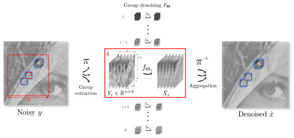
BM3D [9] assumes a locally sparse representation in a transform domain:	NL-Bayes [10] was originally established in the Bayesian setting:	NL-Ridge [11] denoises each patch by linearly combining its most similar noisy patches:
$f_{\Theta_{i}}(Y_{i})=P^{\top}(\Theta_{i}\odot(PY_{i}Q))Q^{\top},$	$f_{\Theta_{i},\beta_{i}}(Y_{i})=\Theta_{i}Y_{i}+\beta_{i}\vec{1}_{k}^{\top},$	$f_{\Theta_{i}}(Y_{i})=Y_{i}\Theta_{i}.$
where $P$ and $Q$ are orthogonal matrices and $\odot$ denotes the Hadamard product.	where $\vec{1}_{k}$ denotes the $k$-dimensional all-ones vector.

Figure 1: Illustration of the parametric view of non-local denoisers. Examples of parameterized functions $f_{\Theta_{i}}$, unequivocally identifying the denoiser, are given whose parameters $\Theta_{i}$ are eventually selected for each group of patches by "internal adaptation" (see equation (6)).

The choice of the local denoising function $f$ remains an open question. Restricting it to be a member of a class of parameterized functions $(f_{\Theta})$, we have proposed in [11] a unified framework to properly select one candidate among the chosen class for each group of patches. Figure 1 gives the underlying parameterized functions for three different denoisers [9, 10, 11]. Formally, adopting an even broader view, a non-local denoiser $\phi_{\boldsymbol{\Theta}}$ taking as input a noisy image $y$ composed of $N$ overlapping patches of size $\sqrt{n}\times\sqrt{n}$ can itself be viewed as a highly parameterized function:

$$\phi_{\boldsymbol{\Theta}}(y)=\pi^{-1}(F_{\boldsymbol{\Theta}}(\pi(y)))$$ (1)

where $\pi$ is an operator that extracts $N$ groups of similar patches, viewed as similarity matrices $(Y_{i})_{i=1}^{N}\in\mathbb{R}^{N\times n\times k}$, $\pi^{-1}$ is its pseudo-inverse (replacing the patches at their initial positions and aggregating them by plain averaging) and $F_{\boldsymbol{\Theta}}=\{f_{\Theta_{i}}\}_{i=1}^{N}$ is the function performing the denoising of all similarity matrices in a parallel fashion with $\boldsymbol{\Theta}=\{\Theta_{i}\}_{i=1}^{N}$. More precisely, $F_{\boldsymbol{\Theta}}:\mathbb{R}^{N\times n\times k}\mapsto\mathbb{R}^{N\times n\times k}$ is a function treating each group independently through $f_{\Theta_{i}}$ which is exclusively dedicated to the $i^{th}$ similarity matrix $Y_{i}$. In the following, we assume that patch grouping operator $\pi$ is ideal and forms the patch groups solely based on the similarity of the underlying noise-free patches, and thus independently of the noise realization. This way, $\pi(y)_{i}$ can be identified as the $i^{th}$ noisy similarity matrix associated to the noise-free one $\pi(x)_{i}$.

Note that the number of parameters of $\phi_{\boldsymbol{\Theta}}$ is $N$ times the number of parameters of a single local denoising function $f_{\Theta_{i}}$. Therefore, its number of parameters grows linearly with the number of patches. As an illustrative example and excluding time optimization tricks, $\boldsymbol{\Theta}\in\mathbb{R}^{N\times n\times k}$ in the case of BM3D [9] because $\Theta_{i}\in\mathbb{R}^{n\times k}$ has the same size as a patch group (see Fig. 1). This represents about a hundred million parameters to be found for a $256\times 256$ image with standard patch and group sizes, $n=8\times 8$ and $k=16$.

2.2 Parameter optimization

In [11], we showed that unsupervised two-step non-local algorithms [9, 10, 11] could be reconciled adopting a local minimal risk point of view to compute parameters $\{\Theta_{i}\}_{i=1}^{N}$ independently. More generally, the ultimate objective is to minimize the global risk defined as:

$$\mathcal{R}_{\boldsymbol{\Theta}}(x)=\mathbb{E}\|\phi_{\boldsymbol{\Theta}}(y)-x\|_{2}^{2},$$ (2)

where $x$ is the clean image supposed known and $y$ is the random vector following the distribution dictated by the given noise model (for example, in the case of additive white Gaussian noise of variance $\sigma^{2}$, $y\sim\mathcal{N}(x,\sigma^{2}I)$ where $I$ is the identity matrix). The mathematical expectation is therefore solely on $y$. In others words, the optimal estimator $\hat{x}=\phi_{\boldsymbol{\Theta}^{\ast}}(y)$ minimizes the risk, i.e.

$$\boldsymbol{\Theta}^{\ast}=\arg\min_{\boldsymbol{\Theta}}\mathcal{R}_{\boldsymbol{\Theta}}(x).$$ (3)

Solving (3) directly is difficult due to the aggregation step via operator $\pi^{-1}$ in (1). Therefore, a (suboptimal) greedy approach is used and aims at minimizing the risk at the individual patch group level, as originally proposed in [11]. This allows the problem to be decomposed into $N$ simpler independent subproblems:

$$\Theta_{i}^{\ast}=\arg\min_{\Theta_{i}}\underbrace{\mathbb{E}\|f_{\Theta_{i}}(Y_{i})-X_{i}\|_{F}^{2}}_{R_{\Theta_{i}}(X_{i})},$$ (4)

where $Y_{i}=\pi(y)_{i}$ and $X_{i}=\pi(x)_{i}$ are the $i^{th}$ noisy and noise-free similarity matrices, respectively, and where $\|\cdot\|_{F}$ denotes the Frobenius norm. For the underlying parameterized functions of [9], [10] and [11] (see Fig. 1), problem (4) has a closed-form solution in the case of additive white Gaussian noise as shown by [11].

2.3 Internal adaptation

Obviously $x$ is unknown in practice as it is precisely what we are looking for. Consequently, the minimization problem (3) cannot actually be solved. However, assuming that a (weak) estimate $\tilde{x}$ of the denoised image (a.k.a. pilot or oracle [3]) is available, the authors of [35] proposed, in the context of deep learning, to substitute it for $x$ in risk expression (2). Formally, the idea is to consider the surrogate:

$$\mathcal{R}_{\boldsymbol{\Theta}}(\tilde{x})=\mathbb{E}\|\phi_{\boldsymbol{\Theta}}(y)-\tilde{x}\|_{2}^{2},$$ (5)

where $y$ follows the distribution imposed by the noise model (for example, in the case of additive white Gaussian noise of variance $\sigma^{2}$, $y\sim\mathcal{N}(\tilde{x},\sigma^{2}I)$).

Originally, this so-called "internal adaptation" technique was viewed as a simple post-processing refinement to boost performances of lightweight networks first trained in a supervised manner [35, 4, 5]. In particular, as argued by their authors [35], "internal adaptation" can be useful when the incoming noisy image $y$ deviates from the general statistics of the training set. However, this technique, as shown in [11], turns out to be at the core of the second stage of state-of-the-art unsupervised two-step denoisers [9, 10, 11] where each local risk defined in (4) is replaced by the empirical one:

$$R_{\Theta_{i}}(\tilde{X}_{i})=\mathbb{E}\|f_{\Theta_{i}}(Y_{i})-\tilde{X}_{i}\|_{F}^{2}$$ (6)

where $Y_{i}=\pi(y)_{i}$ and $\tilde{X}_{i}=\pi(\tilde{x})_{i}$.

As long as the pilot $\tilde{x}$ is not too far from the ground truth image $x$, $\hat{x}=\phi_{\boldsymbol{\Theta}^{\ast}}(y)$ obtained through "internal adaptation" by minimizing (5) may be closer to $x$ than the pilot itself (although there is no mathematical guarantee). In practice, all state-of-the-art two-step denoisers [9, 10, 11] always observe a significant boost in performance using this technique compared to the estimate obtained during their first stage. However, counter-intuitively, repeating the process does not bring much improvement and tends on the contrary to severely degrade the image after a few iterations (see Fig. 2). Therefore, these methods stop directly after a single step of "internal adaptation".

Based on this concept, we introduce below a generalized expression of (1) to overcome the second stage limitation. Using a progressive optimization scheme, the proposed algorithm, when used with linear combinations of patches, enables to considerably improve the denoising performance, making it as competitive as WNNM [12], the best unsupervised method to the best of our knowledge.

Figure 2: Evolution of the PSNR for BM3D [9], NL-Bayes [10] and NL-Ridge [11] algorithms when repeating the "internal adaptation" stage on Set12 dataset with noise level $\sigma=25$. After a remarkable jump of PSNR observed between the first estimate and the second one, obtained with "internal adaptation", the PSNR barely improves thereafter and even decreases.

3 Unsupervised iterative linear combinations of patches

In the following, for the sake of simplicity, we assume an additive white Gaussian noise model of variance $\sigma^{2}$.

3.1 Denoising by iterative linear combinations of patches

We propose to study a class of parameterized functions that generalizes (1):

$$\Phi_{\{\boldsymbol{\Theta}_{m}\}_{m=1}^{M}}(y)=\left[\phi_{\boldsymbol{\Theta}_{M}}\circ\ldots\circ\phi_{\boldsymbol{\Theta}_{1}}\right](y)$$ (7)

where $M\in\mathbb{N}^{\ast}$ and "$\circ$" denotes the function composition operator. In other words, we consider the $M$ times iterated version of function (1). In this work, we focus on group denoising functions of the following form:

$$f_{\Theta_{i}}(Y_{i})=Y_{i}\Theta_{i}$$ (8)

already used in [11] (see Fig. 1). This choice is motivated by the fact that, despite their apparent simplicity, we proved in [11] that considering linear combinations of patches is remarkably efficient for image denoising. Note that when fixing $\boldsymbol{\Theta}_{m}=\{I_{k}\}_{i=1}^{N}$ for $m\geq 2$, where $I_{k}$ denotes the identity matrix of size $k$, the above class of functions coincides with (1) as $f_{I_{k}}$ is the identity function $\operatorname{id}_{\mathbb{R}^{n\times k}}$.

3.2 A progressive scheme for parameter optimization

Following the same approach as for two-step non-local denoisers, our objective is to minimize the quadratic risk:

$$\{\boldsymbol{\Theta}_{m}^{\ast}\}_{m=1}^{M}=\mathop{\arg\min}\limits_{\{\boldsymbol{\Theta}_{m}\}_{m=1}^{M}}\underbrace{\mathbb{E}\|\Phi_{\{\boldsymbol{\Theta}_{m}\}_{m=1}^{M}}(y)-x\|_{2}^{2}}_{\mathcal{R}_{\{\boldsymbol{\Theta}_{m}\}_{m=1}^{M}}(x)}$$ (9)

where $x$ is the ground truth image assumed known for the moment and $y\sim\mathcal{N}(x,\sigma^{2}I)$. The optimal estimator, in the $\ell_{2}$ sense, is then $\hat{x}=\Phi_{\{\boldsymbol{\Theta}_{m}^{\ast}\}_{m=1}^{M}}(y)$.

Solving (9) is much more challenging than minimizing (2) due to the repeated aggregation/extraction steps implicitly contained in expression (7) via $\pi\circ\pi^{-1}$. Indeed, it is worth noting that $[\pi\circ\pi^{-1}](z)\neq z$ for $z\in\mathbb{R}^{N\times n\times k}$ when patches in $z$ are not consistent (i.e. there exists two different patch estimates for the same underlying patch). Therefore, we propose a (suboptimal) progressive approach to approximate the solution of (9) as follows:

$$\left\{\begin{array}[]{l}\displaystyle\boldsymbol{\Theta}^{\ast}_{1}=\mathop{\operatorname{argmin}}\limits_{\boldsymbol{\Theta}_{1}}\mathbb{E}\|\phi_{\boldsymbol{\Theta}_{1}}(y)-y_{1}\|_{2}^{2}\\ \displaystyle\boldsymbol{\Theta}^{\ast}_{2}=\mathop{\operatorname{argmin}}\limits_{\boldsymbol{\Theta}_{2}}\mathbb{E}\|[\phi_{\boldsymbol{\Theta}_{2}}\circ\phi_{\boldsymbol{\Theta}^{\ast}_{1}}](y)-y_{2}\|_{2}^{2}\\ \displaystyle\quad\quad\quad\quad\quad\quad\quad\quad\quad\quad\quad\quad\vdots\\ \displaystyle\boldsymbol{\Theta}^{\ast}_{M}=\mathop{\operatorname{argmin}}\limits_{\boldsymbol{\Theta}_{M}}\mathbb{E}\|[\phi_{\boldsymbol{\Theta}_{M}}\circ\phi_{\boldsymbol{\Theta}^{\ast}_{M-1}}\circ\ldots\circ\phi_{\boldsymbol{\Theta}^{\ast}_{1}}](y)-y_{M}\|_{2}^{2}\\ \end{array}\right.$$ (10)

where $y_{m}=x+\tau_{m}(y-x)$ with $(\tau_{m})_{1\leq m\leq M}$ a strictly decreasing sequence satisfying $0\leq\tau_{m}<1$ and $\tau_{M}=0$ (i.e. $y_{M}=x$). Basically, $\boldsymbol{\Theta}_{m}$ are found iteratively in a way such that composing by a new $\phi_{\boldsymbol{\Theta}_{m}}$ closes the gap even more with the ground truth image $x$. Essentially, the proposed scheme amounts to solving $M$ problems of the form:

$$\boldsymbol{\Theta}^{\ast}_{m}=\arg\min_{\boldsymbol{\Theta}_{m}}\mathbb{E}\|\phi_{\boldsymbol{\Theta}_{m}}(z_{m-1})-y_{m}\|_{2}^{2},$$ (11)

where $z_{m}=[\phi_{\boldsymbol{\Theta}^{\ast}_{m}}\circ\ldots\circ\phi_{\boldsymbol{\Theta}^{\ast}_{1}}](y)$ if $m\geq 1$ and $z_{0}=y$ (note that, by construction, $z_{m}$ is expected to be close to $y_{m}$).

3.3 Resolution when the ground truth is available

In order to solve (11), we adopt a greedy approach by minimizing the quadratic loss at the individual patch group level as done in (4). The problem is then decomposed into as many independent subproblems as there are patch groups:

$$\Theta_{i}^{m\ast}=\arg\min_{\Theta_{i}^{m}}\mathbb{E}\|f_{\Theta_{i}^{m}}(Z_{i}^{m-1})-Y_{i}^{m}\|_{F}^{2},$$ (12)

where $Y_{i}^{m}=\pi(y_{m})_{i}=X_{i}+\tau_{m}(Y_{i}-X_{i})$ with $X_{i}=\pi(x)_{i}$ and $Z_{i}^{m-1}=\pi(z_{m-1})_{i}$.

In its current state, (12) cannot be solved easily as in (4) because the probability distribution of the pixels contained in $Z_{i}^{m-1}$ is intractable. Indeed, the repeated aggregation/extraction steps from which $Z_{i}^{m-1}$ is formed make obtaining its law cumbersome. However, it can be approximated by construction as a convex combination of the $i^{th}$ noisy and noise-free similarity matrices $Y_{i}=\pi(y)_{i}$ and $X_{i}=\pi(x)_{i}$, respectively, that is:

$$Z_{i}^{m-1}\approx X_{i}+t_{i}^{m-1}(Y_{i}-X_{i}),$$ (13)

with $t_{i}^{m-1}\in(0,1]$ to be estimated for each similarity matrix and expected to be close to $\tau_{m-1}$ when $m\geq 2$. Note that for $m=1$, this approximation is in fact exact with $t_{i}^{0}=1$. Denoting $\operatorname{sd}(.)$ the operator that computes the standard deviation of the coefficients of the input random matrix, we have $\operatorname{sd}(Y_{i}-Z^{m-1}_{i})=(1-t_{i}^{m-1})\sigma$. The parameter $t_{i}^{m-1}$ can therefore be estimated by:

$$t_{i}^{m-1}=1-\operatorname{sd}(Y_{i}-Z^{m-1}_{i})/\sigma.$$ (14)

Finally, conceding this small approximation, minimization problem (12) yields a closed-form solution given by (see appendix):

$$\Theta_{i}^{m\ast}=\left(1-\frac{\tau_{m}}{t_{i}^{m-1}}\right)\left(X_{i}^{\top}X_{i}+n(t_{i}^{m-1}\sigma)^{2}I_{k}\right)^{-1}X_{i}^{\top}X_{i}+\frac{\tau_{m}}{t_{i}^{m-1}}I_{k}.$$ (15)

3.4 Use of M cost-efficient pilots for unsupervised resolution

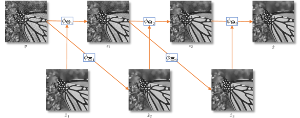
Figure 3: Illustration of the proposed scheme based on the use of $M=3$ pilots for unsupervised optimization.

Obviously solving the initial objective (9) is impossible in practice, whatever the scheme of optimization adopted, as the ground truth image $x$ is missing. In section 2, we have mentioned that substituting a pilot $\tilde{x}$ for $x$, that is applying "internal adaptation" [35], constitutes the reference method to overcome this issue when $M=1$. In the general case, we propose to use $M$ different pilots $\tilde{x}_{1},\ldots,\tilde{x}_{M}$. More precisely, pilot $\tilde{x}_{m}$ is dedicated to the computation of $\boldsymbol{\Theta}^{\ast}_{m}$ as follows:

• $X_{i}=\pi(x)_{i}$ is replaced by $\tilde{X}^{m}_{i}=\pi(\tilde{x}_{m})_{i}$.

• $t_{i}^{m-1}$ is computed using the sample standard deviation in (14) where $Y_{i}=\pi(y)_{i}$ and $Z_{i}^{m-1}=\pi(z_{m-1})_{i}$ are the only realizations at our disposal.

• $\Theta_{i}^{m\ast}$ is finally computed with (15).

Let us assume that, for $m\geq 1$, $\boldsymbol{\Theta}^{\ast}_{1},\ldots,\boldsymbol{\Theta}^{\ast}_{m-1}$ have already been computed and that pilot $\tilde{x}_{m}$ is available. Then, $\boldsymbol{\Theta}^{\ast}_{m}$ can be computed using this pilot and we propose to use an updated one for the next step of the form:

$$\tilde{x}_{m+1}=[\phi_{\boldsymbol{\Xi}_{m}}\circ\phi_{\boldsymbol{\Theta}^{\ast}_{m-1}}\circ\ldots\circ\phi_{\boldsymbol{\Theta}^{\ast}_{1}}](y)=\phi_{\boldsymbol{\Xi}_{m}}(z_{m-1}).$$ (16)

where parameters $\boldsymbol{\Xi}_{m}$ are to be found. Ideally, we want:

$$\boldsymbol{\Xi}^{\ast}_{m}=\arg\min_{\boldsymbol{\Xi}_{m}}\mathbb{E}\|\phi_{\boldsymbol{\Xi}_{m}}(z_{m-1})-x\|_{2}^{2}$$ (17)

for which the solution is given, according to (15) with $\tau_{m}=0$, by:

$$\boldsymbol{\Xi}^{\ast}_{m}=\left\{\left(X_{i}^{\top}X_{i}+n(t_{i}^{m-1}\sigma)^{2}I_{k}\right)^{-1}X_{i}^{\top}X_{i}\right\}_{i=1}^{N}$$ (18)

But, as $x$ is unknown in practice, $X_{i}=\pi(x)_{i}$ is replaced by the latest pilot at our disposition, that is $\tilde{X}^{m}_{i}=\pi(\tilde{x}_{m})_{i}$, and sample standard deviation is used for the computation of $t_{i}^{m-1}$ in (14). This way, provided that an initial pilot $\tilde{x}_{1}$ is available, all set of matrices from $\boldsymbol{\Theta}^{\ast}_{1}$ to $\boldsymbol{\Theta}^{\ast}_{M}$ can be computed iteratively with updated pilots at each step to finally get $\hat{x}=\Phi_{\{\boldsymbol{\Theta}_{m}^{\ast}\}_{m=1}^{M}}(y)=z_{M}$ as the final estimate for $x$. As for the choice of the initial pilot $\tilde{x}_{1}$, the reader is referred to section 4 in this regard. Figure 3 illustrates the proposed scheme for unsupervised resolution based on the use of $M$ different pilots.

We want to emphasize that using the $M$ proposed pilots instead of a single one for each step does not add much in terms of computational cost, while improving a lot the estimation process. Indeed, the cost for computing the $\boldsymbol{\Xi}^{\ast}_{m}$ can be immediately recycled to compute the $\boldsymbol{\Theta}^{\ast}_{m}$ at the same time:

$$\boldsymbol{\Theta}^{\ast}_{m}=\left\{(1-\frac{\tau_{m}}{t_{i}^{m-1}})\Xi_{i}^{m\ast}+\frac{\tau_{m}}{t_{i}^{m-1}}I_{k}\right\}_{i=1}^{N}$$ (19)

The whole detailed procedure is summarized in Algorithm 1 where patch grouping is performed on $z_{m}$ at each step $m$.

Algorithm 1 LIChI: Linear and Iterative Combinations of patcHes for Image denoising

Noisy image $y$, initial pilot $\tilde{x}_{1}$, noise level $\sigma$, group size $k$, patch size $\sqrt{n}$, number of iterations $M$, sequence $(\tau_{i})_{1\leq i\leq M}$.

Denoised image $\hat{x}$.

$z_{0}=y$

for $m=1$ to $M$ do

     for each $\sqrt{n}\times\sqrt{n}$ patch in $z_{m-1}$ indexed by $i$ do

         Find its $k$ most similar patches in $z_{m-1}$ to form similarity matrix $Z^{m-1}_{i}$.

         Form $\tilde{X}^{m}_{i}$ and $Y^{m}_{i}$ with the corresponding patches in $\tilde{x}_{m}$ and $y$, respectively.

         $\displaystyle t_{i}^{m-1}=1-\operatorname{sd}(Y^{m}_{i}-Z^{m-1}_{i})/\sigma$

         $\displaystyle\Xi_{i}^{m}=\left(\tilde{X}_{i}^{m\top}\tilde{X}^{m}_{i}+n(t_{i}^{m-1}\sigma)^{2}I_{k}\right)^{-1}\tilde{X}_{i}^{m\top}\tilde{X}^{m}_{i}$

         $\displaystyle\tilde{X}^{m+1}_{i}=Z^{m-1}_{i}\Xi_{i}^{m}$

         $\displaystyle\Theta_{i}^{m}=(1-\frac{\tau_{m}}{t_{i}^{m-1}})\Xi_{i}^{m}+\frac{\tau_{m}}{t_{i}^{m-1}}I_{k}$

         $\displaystyle Z^{m}_{i}=Z^{m-1}_{i}\Theta_{i}^{m}$

     end for

     Reposition and aggregate patches of each patch group $Z^{m}_{i}$ and $\tilde{X}^{m+1}_{i}$ to form $z_{m}$ and updated pilot $\tilde{x}_{m+1}$.

end for

return $z_{M}$

4 Building an initial pilot

In Algorithm 1, an initial pilot $\tilde{x}_{1}$ is necessary. If in theory, any denoiser can be used to that end, we show in this section how to build one of the form $\tilde{x}_{1}=\phi_{\boldsymbol{\Theta}}(y)$ where linear combinations of patches is once again leveraged for local denoising (8). The denoisers that we consider in this section are then described by Algorithm 2, all differing in the estimation of the parameters $\boldsymbol{\Theta}=\{\Theta_{i}\}_{i=1}^{N}$ corresponding to the combination weights.

Algorithm 2 Pilot initialization by linear combinations of patches

Noisy image $y$, noise level $\sigma$, group size $k$, patch size $\sqrt{n}$.

Pilot image $\tilde{x}$.

for each $\sqrt{n}\times\sqrt{n}$ patch in $y$ indexed by $i$ do

     Find its $k$ most similar patches in $y$ to form similarity matrix $Y_{i}$.

     Compute combination weights $\Theta_{i}$ with (21), (26), (27) or (28).

     $\tilde{X}_{i}=Y_{i}\Theta_{i}$.

end for

Reposition and aggregate patches of each patch group $\tilde{X}_{i}$ to form the pilot image $\tilde{x}$.

return $\tilde{x}$

4.1 Stein’s unbiased risk estimate (SURE)

Considering the same risk minimization problem as (2) for the optimization of $\boldsymbol{\Theta}=\{\Theta_{i}\}_{i=1}^{N}$ brings us back to the study of the $N$ independent subproblems of the form (4). However, this time we aim to minimize each local risk by getting rid of any surrogate for the ground truth similarity matrices $X_{i}$. Stein’s unbiased risk estimate (SURE) provides such an opportunity. Indeed, this popular technique in image denoising [26, 27, 28] gives an estimate of the risk $R_{\Theta_{i}}(X_{i})$ that solely depends on the observation $Y_{i}$. In the case of linear combinations of patches (8), the computation of SURE yields (see appendix):

$$-kn\sigma^{2}+\|Y_{i}\Theta_{i}-Y_{i}\|_{F}^{2}+2n\sigma^{2}\operatorname{tr}(\Theta_{i}),$$ (20)

where $\operatorname{tr}(.)$ denotes the trace operator. Substituting this estimate for the risk $R_{\Theta_{i}}(X_{i})$ and minimizing it with regards to $\Theta_{i}$, we get:

$$\Theta_{i}^{\text{SURE}}=\left(Y_{i}^{\top}Y_{i}\right)^{-1}\left(Y_{i}^{\top}Y_{i}-n\sigma^{2}I_{k}\right).$$ (21)

Note that $\Theta_{i}^{\text{SURE}}$ is close to the parameters $\Theta_{i}^{\ast}$ minimizing the risk as long as the variance of SURE is low. A rule of thumbs used in [26] states that the number of parameters must not be "too large" compared to the number of data in order for the variance of SURE to remain small. In our case, this suggests that $n>k$. In other words, a small amount of large patches are necessary for this technique. Finally, a possible pilot for $x$ is $\tilde{x}_{1}=\phi_{\boldsymbol{\Theta}^{\text{SURE}}}(y)$ with $\boldsymbol{\Theta}^{\text{SURE}}=\{\Theta^{\text{SURE}}_{i}\}_{i=1}^{N}$.

4.2 Noisier2Noise

Although somewhat counter-intuitive, the authors of [29] showed, in a deep-learning context, that training a neural network to recover the original noisy image from a noisier version (synthetically generated by adding extra noise) constitutes an efficient way to learn denoising weights without access to any clean training examples. Drawing a parallel, this amounts in our case to considering the minimization of the following risk:

$$\mathcal{R}_{\boldsymbol{\Theta}}(y)=\mathbb{E}\|\phi_{\boldsymbol{\Theta}}(z)-y\|_{2}^{2},$$ (22)

where $y$ is the only noisy observation at our disposal and $z$ is the noisier random vector following the probability distribution dictated by the chosen extra-noise model. In particular, in the case of additive white Gaussian noise of variance $(\alpha\sigma)^{2}$, where $\alpha>0$ is an hyperparameter controlling the amount of extra noise, $z\sim\mathcal{N}(y,(\alpha\sigma)^{2}I)$. Mathematically speaking, minimizing (22) is no more difficult than minimizing (2) and the same greedy approximation used in (4) can be applied bringing us to solve the $N$ independent local subproblems:

$$\hat{\Theta}_{\alpha,i}=\arg\min_{\Theta_{i}}\;\mathbb{E}\|f_{\Theta_{i}}(Z_{i})-Y_{i}\|_{F}^{2},$$ (23)

where $Z_{i}=\pi(z)_{i}$ and $Y_{i}=\pi(y)_{i}$. As showed by [11], problem (23) amounts to solving a multivariate ridge regression and the closed-form solution is:

$$\hat{\Theta}_{\alpha,i}=\left(Y_{i}^{\top}Y_{i}+n(\alpha\sigma)^{2}I_{k}\right)^{-1}Y_{i}^{\top}Y_{i}.$$ (24)

To get an estimate of the noise-free image $x$, Noisier2Noise [29] suggests to compute:

$$\frac{(1+\alpha^{2})\phi_{\hat{\boldsymbol{\Theta}}_{\alpha}}(z)-z}{\alpha^{2}}$$ (25)

where $\hat{\boldsymbol{\Theta}}_{\alpha}$ is the minimizer of (22) approached by $\{\hat{\Theta}_{\alpha,i}\}_{i=1}^{N}$. In appendix, we show that this quantity is equal to $\phi_{\boldsymbol{\Theta}_{\alpha}^{\text{}}}(y)$ on average with $\boldsymbol{\Theta}_{\alpha}^{\text{Nr2N}}=\{\Theta^{\text{Nr2N}}_{\alpha,i}\}_{i=1}^{N}$ where:

$$\Theta^{\text{Nr2N}}_{\alpha,i}=\left(Y_{i}^{\top}Y_{i}+n(\alpha\sigma)^{2}I_{k}\right)^{-1}\left(Y_{i}^{\top}Y_{i}-n\sigma^{2}I_{k}\right).$$ (26)

The choice of the hyperparameter $\alpha$ remains an open question. The authors of [29] recommend the value $\alpha=0.5$ that works well for a variety of noise levels in their experiments. This is the value that we use for all our experiments thereafter. Interestingly, for $\alpha\rightarrow 0$, parameters $\boldsymbol{\Theta}_{\alpha}^{\text{Nr2N}}$ converge to $\boldsymbol{\Theta}^{\text{SURE}}$. A practical advantage of $\boldsymbol{\Theta}_{\alpha}^{\text{Nr2N}}$ over $\boldsymbol{\Theta}^{\text{SURE}}$ is that the matrices $Y_{i}^{\top}Y_{i}+n(\alpha\sigma)^{2}I_{k}$ in (26) are symmetric positive-definite and therefore invertible, contrary to $Y_{i}^{\top}Y_{i}$ in (21) which is only positive semi-definite and positive-definite almost surely in the case of ideal additive white Gaussian noise when $n\geq k$. For real-world noisy images, estimation through combination weights $\boldsymbol{\Theta}_{\alpha}^{\text{Nr2N}}$ is recommended over $\boldsymbol{\Theta}^{\text{SURE}}$ as, in some cases, matrices $Y_{i}^{\top}Y_{i}$ may not be invertible.

Note that the same weight expressions as (26) can also be obtained within the Recorrupted-to-recorrupted [34] paradigm, which was originally applied in a deep-learning context, and that provides an unbiased estimate of a risk close to (4).

4.3 Two additional extreme pilots

In the case where the noisy patches within a group $Y_{i}$ are originally strictly identical (perfect patch group), the optimal weights are the one computing a plain averaging (see appendix):

$$\Theta_{i}^{\text{AVG}}=\vec{1}_{k}\vec{1}_{k}^{\top}/k$$ (27)

where $\vec{1}_{k}$ denotes the $k$-dimensional all-ones vector. Under the optimistic assumption that each patch group formed is perfect, the pilot $\tilde{x}_{1}=\phi_{\boldsymbol{\Theta^{\text{AVG}}}}(y)$ with $\Theta^{\text{AVG}}=\{\Theta_{i}^{\text{AVG}}\}_{i=1}^{N}$ is then optimal.

On the contrary, when the patch groups formed are highly dissimilar, collaborative denoising cannot be beneficial and the resulting "do-nothing" weights are:

$$\Theta_{i}^{\text{Noisy}}=I_{k}.$$ (28)

where $I_{k}$ is the identity matrix of size $k$. Under this pessimistic assumption, the pilot $\tilde{x}_{1}=\phi_{\boldsymbol{\Theta}^{\text{Noisy}}}(y)=y$ is optimal. This in fact amounts to consider the original noisy image itself as an initial pilot for Algorithm 1.

4.4 Comparison of the pilots

Figure 4: Average PSNR (in dB) results on patch groups (dotted line), after aggregation (dashed line) and when taken as input for Algorithm 1 (solid line) for Set12 dataset depending on combination weights used and noise level. Patch and group sizes are chosen as indicated by Table 1.

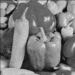
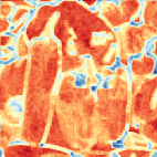
Noisy ($\sigma=15$)	Average / 26.83 dB	SURE / 25.43 dB	Noisier2Noise / 28.06 dB

Figure 5: Colormap of the PSNR (in dB) of the denoised similarity matrices ($n=7\times 7$ and $k=18$) associated with each overlapping patch of the noisy image. The average PSNR on similarity matrices is also indicated.

To study the performance of the proposed pilots, we compare them at three different levels: at the individual patch group level, at the global level after the aggregation stage and finally, most importantly, when taken at input for Algorithm 1. Figure 4 displays the average PSNR results obtained for these three criteria at different noise levels on a popular image dataset. Although the studied pilots have very different behaviors at the patch group level, they tend to give similar results when taken as input for Algorithm 1. The "do-noting" weights (28), however, perform slightly worse than the other three, especially at high noise levels, while the averaging ones (27) are disappointing at low noise levels. As for SURE (21) and Noisier2Noise (26) weights, they give almost identical results in the end even if the Noisier2Noise weights are much more efficient on the similarity matrices. By the way, this highlights a non-intuitive phenomenon which was already observed in [4]: being efficient at the patch scale is a sufficient but not necessary condition to be efficient after the aggregation stage. This confirms that aggregation is not a basic post-processing step but plays a crucial role in image denoising.

Figure 5 provides a visual comparison of the performance of the different combination weights depending on the location of the reference patch for intermediate noise level. Unsurprisingly, combination weights (27) are extremely effective on the smooth parts of the image because they are theoretically optimal when applied on groups of patches being originally identical (see appendix). However, when patch groups are less homogeneous, which occurs when the reference patch is a rare patch, averaging over inherently dissimilar patches severely affects restoration. On the contrary, SURE (21) and Noisier2Noise (26) weights seem to be more versatile and less sensitive to the homogeneity of the similarity matrices, yielding comparable reconstruction errors regardless of the rarity of the reference patch.

4.5 The crucial role of the aggregation stage

Number of estimates used per pixel	AVG (27.62 dB / 27.93 dB)	SURE (25.64 dB / 31.52 dB)	Nr2N (28.79 dB / 31.83 dB)

Figure 6: Image denoising of Castle image from BSD68 dataset ($\sigma=15$) by Algorithm 2 for three different combinations weights: (21) , (26) and (27). Right: a single estimate per pixel (no aggregation), left: aggregation by averaging all estimates per pixel.

To get a better understanding of the role of the aggregation stage, we define $\psi_{\boldsymbol{\Theta}}(y)$ as the estimator that skips it:

$$\psi_{\boldsymbol{\Theta}}(y)=\rho(F_{\boldsymbol{\Theta}}(\pi(y)))$$ (29)

where operator $\rho$ replaces each patch at their initial location and selects a single estimate among those available for a given pixel. The single estimate is arbitrarily chosen at random from the most central pixels of the denoised reference patches to avoid considering poor quality estimates. In particular, when the patch size $\sqrt{n}$ is an odd number, the chosen estimates are the denoised central pixels of the reference patches. Figure 6 illustrates the gap of performance between $\psi_{\boldsymbol{\Theta}}(y)$ and $\phi_{\boldsymbol{\Theta}}(y)$ for combination weights (21), (26) and (27). Skipping the aggregation step results in a much poorer estimation, especially for weights (21) and (26). As a matter of fact, non-local methods have the particularity of producing a large number of estimates per noisy pixel, up to a few thousand (see Fig. 6), because a noisy pixel can appear in many similarity matrices and even several times in one. To study the benefit of exploiting those multiple estimates, a bias-variance decomposition can be leveraged:

$$\underbrace{\mathbb{E}\|\tilde{x}-x\|_{2}^{2}/d}_{\text{MSE}}=\underbrace{\|\mathbb{E}(\tilde{x})-x\|_{2}^{2}/d}_{\text{squared-bias}}+\underbrace{\mathbb{E}\|\tilde{x}-\mathbb{E}(\tilde{x})\|_{2}^{2}/d}_{\text{variance}}$$ (30)

where $\tilde{x}$ is the estimator for the ground truth image $x$. Figure 7 highlights the bias–variance tradeoff for estimators $\psi_{\boldsymbol{\Theta}}(y)$ and $\phi_{\boldsymbol{\Theta}}(y)$ and combination weights (21), (26) and (27) where $y$ is the noisy image shown in Fig. 3. We can notice that the squared-bias part of the MSE in (30) is practically unchanged whether aggregation is applied or not. However, a remarkable drop in variance is notable. This is particularly impressive for SURE estimator (21), which significantly reduces its variance and so its MSE thanks to aggregation, closing the gap with the Noisier2Noise estimator (26) as they share almost the same squared-bias. However, for averaging estimator (27), the variance represents a very small part in the MSE decomposition (30) and so aggregation is not beneficial.

Figure 7: Bias-variance tradeoff between estimators (1) and (29), i.e. with (w/) and without (w/o) aggregation, for three different types of combination weights. Results obtained with noisy image shown in Fig. 3 at noise level $\sigma=20$ with patch size $n=9\times 9$ and group size $k=18$, estimated via Monte-Carlo simulation using $100$ different realizations of the noise.

We can draw a parallel with a popular machine-learning ensemble meta-algorithm: bootstrap aggregating, also called bagging [16]. Bagging consists of fitting several (weak) models to sampled versions of the original training dataset (bootstrap) and combining them by averaging the outputs of the models during the testing phase (aggregation). This procedure is known for improving model performance, as it decreases the variance of the model, without increasing the squared-bias. In our case, the bootstrap samples can be materialized by the numerous noisy similarity matrices $Y_{i}$ on which (weak) models $f_{\Theta_{i}}(.)$ are trained in an unsupervised manner. Combining pixel estimates by aggregation enables to significantly reduce the variance while keeping the squared-bias unchanged.

5 Experimental results

In this section, we compare the performance of the proposed method, referred to as LIChI (Algorithm 1), with state-of-the-art methods, including related deep-learning-based methods [19, 20, 35, 30, 31, 32] applied to standard gray images artificially corrupted with additive white Gaussian noise with zero mean and variance $\sigma^{2}$ but also real-world noisy images. The implementations provided by the authors were used for all algorithms. Performances of LIChI and other methods are assessed in terms of PSNR values when the ground truth is available. The code can be downloaded at: https://github.com/sherbret/LIChI/.

5.1 Setting of algorithm parameters

In all our experiments, the patch size $n$, the group size $k$ and the strictly decreasing sequence $(\tau_{m})_{1\leq m\leq M}$ in algorithm 1 are empirically chosen as $n=6\times 6$, $k=64$ and $\tau_{m}=0.75\times(1-m/M)$, respectively. As for the number of iterations $M$, its value depends on the noise level $\sigma$: the higher the noise level, the more iterations of linear combinations of patches are necessary. Moreover, its optimal value is also influenced by the quality of the initial pilot, itself dependent on patch and group sizes according to algorithm 2. In Table 1, we report, for each noise range, the recommended patch size $n$ and group size $k$ in algorithm 2 for deriving the first pilot $\tilde{x}$ with Noisier2Noise weights as this the most relevant choice based on the experiments in section 4, and the associated number of iterations $M$.

Table 1: Recommended patch size $n$ and group size $k$ for Algorithm 2 and corresponding number of iterations $M$ in Algorithm 1.

$\sigma$	$n$	$k$	$M$
${\color[rgb]{1,1,1}1}0<\sigma\leq 10$	$9\times 9$	16	6
$10<\sigma\leq 30$	$11\times 11$	16	9
$30<\sigma\leq 50$	$13\times 13$	16	11

For the sake of computational efficiency, the search for similar patches, computed in the $\ell_{2}$ sense, across the image is restricted to a small local window $w\times w$ centered around each reference patch (in our experiments $w=65$). Considering iteratively each overlapping patch of the image as reference patch is also computationally demanding, therefore only an overlapping patch over $\delta$, both horizontally and vertically, is considered as a reference patch. The number of reference patches and thus the time spent searching for similar patches is then divided by $\delta^{2}$. This common technique [9, 11, 12] is sometimes referred in the literature as the step trick. In our experiments, we take $\delta=3$. Finally, to further speed up the algorithm, the search for the location of patches similar to the reference ones is only performed every third iteration because, in practice, the calculated locations vary little from one iteration to the next.

5.2 Results on artificially noisy images

We tested the denoising performance of our method on three well-known datasets: Set12, BSD68 [36] and Urban100 [37]. Figure 8 provides a qualitative comparison with other state-of-the-art algorithms. LIChI compares favorably with the very best methods, including DnCNN [19] which is the most cited supervised neural network for image denoising. In particular, this neural network, contrary to our method, is unable to recover properly the stripes on Barbara image, probably because such structures were not present in its external training dataset. Moreover, the benefit of iterating linear combinations, compared to the one-pass version represented by NL-Ridge [11] is clearly visible. Indeed, many eye-catchy artifacts, especially around the edges, are removed and the resulting denoised image is much more pleasant and natural.

Table 2: The PSNR (dB) results of different methods on three datasets corrupted with synthetic white Gaussian noise and $\sigma=5$, $15$, $25$, $35$ and $50$. Best among each category (unsupervised or supervised) is in bold. Best among each subcategory is underlined.

|c@  c@  c c@      c@  c@  c@  c@  c@  c@  c@  c@  c@       c@  c@  c@  c@  c@  c@  c@  c@  c@       c@  c@  c@  c@  c@  c@  c@  c@  c@ c| Methods Set12 BSD68 Urban100

Noisy 34.25 / 24.61 / 20.17 / 17.25 / 14.15 34.25 / 24.61 / 20.17 / 17.25 / 14.15 34.25 / 24.61 / 20.17 / 17.25 / 14.15

Unsupervised Traditional 2-step BM3D [9] 38.02 / 32.37 / 29.97 / 28.40 / 26.72 37.55 / 31.07 / 28.57 / 27.08 / 25.62 38.30 / 32.35 / 29.70 / 27.97 / 25.95
NL-Bayes [10] 38.12 / 32.25 / 29.88 / 28.30 / 26.45 37.62 / 31.16 / 28.70 / 27.18 / 25.58 38.33 / 31.96 / 29.34 / 27.61 / 25.56

NL-Ridge [11] 38.19 / 32.46 / 30.00 / 28.41 / 26.73 37.67 / 31.20 / 28.67 / 27.14 / 25.67 38.56 / 32.53 / 29.90 / 28.13 / 26.29

3-32

M-step

WNNM [12] 38.36 / 32.70 / 30.26 / 28.69 / 27.05 37.80 / 31.37 / 28.83 / 27.30 / 25.87 - / 32.97 / 30.39 / - / 26.83

LIChi 38.36 / 32.71 / 30.24 / 28.61 / 26.81 37.80 / 31.41 / 28.86 / 27.31 / 25.72 38.77 / 33.00 / 30.37 / 28.59 / 26.56

2-32

Deep learning DIP [30] - / 30.12 / 27.54 / - / 24.67 - / 28.83 / 26.59 / - / 24.13 - / - / - / - / -
Noise2Self [31] - / 31.01 / 28.64 / - / 25.30 - / 29.46 / 27.72 / - / 24.77 - / - / - / - / -

Self2Self [32] - / 32.07 / 30.02 / - / 26.49 - / 30.62 / 28.60 / -/ 25.70 - / - / - / - / -

Supervised DnCNN [19] - / 32.86 / 30.44 / 28.82 / 27.18 - / 31.73 / 29.23 / 27.69 / 26.23 - / 32.68 / 29.97 / 28.11 / 26.28
FFDNet [20] 38.11 / 32.75 / 30.43 / 28.92 / 27.32 37.80 / 31.63 / 29.19 / 27.73 / 26.29 38.12 / 32.43 / 29.92 / 28.27 / 26.52
LIDIA [35] - / 32.85 / 30.41 / -/ 27.19 - / 31.62 / 29.11 / -/ 26.17 - / 32.80 / 30.12 / - / 26.51
DCT2net [4] 37.65 / 32.10 / 29.71 / 28.10 / 26.39 37.34 / 31.09 / 28.64 / 27.17 / 25.68 37.59 / 31.48 / 28.81 / 27.04 / 25.17

PSNR results are reported in Table 5.2 on the three datasets considered at different noise levels. For the sake of a fair comparison, algorithms are divided into two categories: unsupervised methods, meaning that these algorithms only have access to the input noisy image (either traditional or deep learning-based), and supervised ones (i.e. deep neural networks) that require a training phase beforehand on an external dataset. Note that only the single-image extension was considered for Noise2Self [31] and the time-consuming "internal adaptation" option was not used for LIDIA [35]. Results show that, although simpler conceptually, LIChI is as efficient as WNNM [12], the best unsupervised denoiser, to the best of our knowledge. This proves that considering iterative linear combinations of noisy patches is enough to reach state-of-the-art performances. However, for very high noise levels ($\sigma\geq 50$), our method seems to lose some of its effectiveness and the low-rank paradigm adopted by WNNM [12] is objectively better. Finally, it is interesting to notice that, on Urban100 [37] dataset which contains abundant structural patterns and textures, all supervised neural networks are outperformed by the best unsupervised methods.

Noisy / 22.09 dB	Ground truth BM3D / 31.72 dB NL-Ridge / 32.07 dB DnCNN / 31.06 dB WNNM / 32.16 dB LIChI (ours) / 32.15 dB
Noisy / 22.09 dB	Ground truth BM3D / 36.76 dB NL-Ridge / 36.82 dB DnCNN / 37.06 WNNM / 36.95 dB LIChI (ours) / 37.18 dB
Noisy / 22.09 dB	Ground truth BM3D / 29.50 dB NL-Ridge / 29.99 dB DnCNN / 30.06 WNNM / 30.94 dB LIChI (ours) / 30.99 dB

Figure 8: Qualitative comparison of image denoising results with synthetic white Gaussian noise ($\sigma=20$). Zoom-in regions are indicated for each method. From top to bottom: Barbara from Set12, Img009 from Urban100 and Img019 from Urban100.

Noisy	Noisy BM3D [9] NL-Ridge [11] FFDNet [20] WNNM [12] LIChI (ours)
Noisy	Noisy BM3D [9] NL-Ridge [11] FFDNet [20] WNNM [12] LIChI (ours)
Noisy	Noisy BM3D [9] NL-Ridge [11] FFDNet [20] WNNM [12] LIChI (ours)

Figure 9: Qualitative comparison of image denoising results on real-world noisy images from Darmstadt Noise Dataset [33]. Zoom-in regions are indicated for each method. From top to bottom: Img0003, Img0037 and Img0044.

5.3 Results on real-world noisy images

We also tested the proposed method on the Darmstadt Noise Dataset [33] which is a dataset composed of $50$ real-noisy images. It relies on taking sets of images of a static scene with different ISO values, where the nearly noise-free low-ISO image is carefully post-processed to derive the ground-truth. To make this dataset even more realistic, ground-truth images are hidden from the users to avoid any bias in the evaluation. To compute standard metrics on denoised images, the user has to upload them on the official website where the computation is done automatically.

The real noise can be modeled as a Poisson-Gaussian noise, itself approximated with a heteroscedastic Gaussian noise whose variance is intensity-dependent:

$$y=\mathcal{N}(x,\operatorname{diag}(ax+b))$$ (31)

where $(a,b)\in\mathbb{R}^{+}\times\mathbb{R}^{+}$ are the noise parameters and operator $\operatorname{diag}(.)$ constructs the diagonal matrix associated to the input vector. For each noisy image, the authors of [33] calculated the adequate noise parameters $(a,b)$ based on this model and made them available to the user. To apply Gaussian denoisers on these noisy images, and in particular the proposed method, a stabilization of variance is necessary. We used the generalized Anscombe transform [6] to that end as in [33].

Table 3: Results for denoising on raw data with VST on Darmstadt Noise Dataset (DND)

	Unsupervised						Supervised
Methods	BM3D [9]	NL-Ridge [11]	KSVD [7]	NCSR [14]	WNNM [12]	LIChI	MLP [25]	TNRD [22]	FFDNet [20]	DCT2net [4]
PSNR (in dB)	47.15	47.01	46.87	47.07	47.05	47.35	45.71	45.70	47.40	46.83

Figure 9 shows a qualitative comparison of the results obtained with state-of-the-art Gaussian denoisers. Since the real noise is relatively low, it is difficult to really differentiate between all methods. However, the good news is that this experiment proves that Gaussian denoisers are able to handle real noise in a decent way via variance stabilization. Table 3 compares the average PSNR obtained on this dataset for different methods. LIChI obtains the second best score, surpassing BM3D [9] which was so far the best unsupervised method on this dataset, and further closing the gap with FFDNet [20], a supervised neural network trained on a large set of images artificially corrupted with Gaussian noise.

5.4 Complexity

We want to emphasize that LIChI, though being an iterative algorithm, is relatively fast compared to its traditional and deep-learning-based unsupervised counterparts. In Table 5.4, we reported the running time of different state-of-the-art algorithms. It is provided for information purposes only, as the implementation, the language used and the machine on which the code is run, highly influence the execution time. The CPU used is a 2,3 GHz Intel Core i7 and the GPU is a GeForce RTX 2080 Ti. Note that LIChI has been entirely implemented in Python with Pytorch, enabling it to run on GPU unlike its traditional counterparts. The gap in terms of running time between supervised and unsupervised methods is explained by the fact that these latter solve optimization problems on the fly. In comparison, supervised methods find optimal parameters for empirical risk minimization in advance on an external dataset composed of clean/noisy images and this time for optimization, sometimes counting in days on a GPU, is not taking into account in Table 5.4. Nevertheless, note that traditional unsupervised methods are much less computationally demanding than deep-learning-based ones because, unlike the latter which use the time-consuming gradient descent algorithm for optimization, traditional ones have closed-form solutions.

Table 4: Running time (in seconds) of different methods for an image of size $256\times 256$. Best among each category (unsupervised or supervised) is in bold. Best among each subcategory is underlined.

|c@  c@  c c@      c@  c@  c@  c|

Methods CPU / GPU

Unsupervised Traditional 2-step BM3D [9] 1.68 / -

NL-Bayes [10] 0.21 / -

NL-Ridge [11] 0.66 / 0.162

3-8

M-step WNNM [12] 63.31 / -

LIChI 11.42 / 1.08

2-8

Deep learning DIP [30] - / $\sim$ 5 min
Noise2Self [31] - / $\sim$ 5 min
Self2Self [32] - / $\sim$ 1 hr

Supervised DnCNN [19] 0.35 / 0.007
FFDNet [20] 0.06 / 0.001
LIDIA [35] 21.08 / 1.18
DCT2net [4] 0.18 / 0.007

6 Conclusion

We presented a parametric unified view of non-local denoisers, with BM3D in the foreground, and extended their underlying formulation by iteration. Within this paradigm and using quadratic risk minimization, we proposed a progressive approach to find the optimal parameters in an unsupervised manner. We derive LIChI algorithm, which exploits iterative non-local linear combinations of patches. Our experimental results show that LIChI preserves much better structural patterns and textures and generates much less visual artifacts, in particular around the edges, than single-iterated denoisers, such as BM3D. The proposed algorithm compares favorably with WNNM, the best unsupervised denoiser to the best of our knowledge, both in terms of both quantitative measurement and visual perception quality, while being faster at execution.

A possible extension of our work would be to adapt the proposed iterative formulation to other parametric group denoising functions than linear combinations. If in our experiments, only the latter produced significant improvements over the single-iterated version, the door remains open for other, possibly better, initiatives.

7 Appendix

7.1 Proofs of the article

In what follows, $X,Y\in\mathbb{R}^{n\times k}$ with $Y_{i,j}\sim{\cal N}(X_{i,j},\sigma^{2})$ independent along each row and $f_{\Theta}:Y\mapsto Y\Theta$ with $\Theta\in\mathbb{R}^{k\times k}$.

Lemma 1.

Let $A\in\mathbb{R}^{n\times k}$, $\lambda\in\mathbb{R}^{+}$ and $\mu\in\mathbb{R}$. If $A^{\top}A$ is invertible or $\lambda>0$:

$$\mathop{\arg\min}\limits_{\Theta\in\mathbb{R}^{k\times k}}\|A\Theta-A\|_{F}^{2}+\lambda\|\Theta\|_{F}^{2}+2\mu\operatorname{tr}(\Theta)=(A^{\top}A+\lambda I_{k})^{-1}(A^{\top}A-\mu I_{k}).$$

Proof.

Let $H:\Theta\in\mathbb{R}^{k\times k}\mapsto\|A\Theta-A\|_{F}^{2}+\lambda\|\Theta\|_{F}^{2}+2\mu\operatorname{tr}(\Theta)$ and $\displaystyle h_{j}:\theta\in\mathbb{R}^{k}\mapsto\|A\theta-A_{\cdot,j}\|_{2}^{2}+\lambda\|\theta\|_{2}^{2}+2\mu\theta_{j}$ such that

$$H(\Theta)=\sum_{j=1}^{k}h_{j}(\Theta_{\cdot,j}).$$

Then, as $A^{\top}A+\lambda I_{k}$ is symmetric positive definite and thus invertible, we have:

$$\nabla h_{j}(\theta)=2A^{\top}(A\theta-A_{\cdot,j})+2\lambda\theta+2\mu e_{j}=0\Leftrightarrow\theta=(A^{\top}A+\lambda I_{k})^{-1}(A^{\top}A_{\cdot,j}-\mu e_{j}),$$

and finally,

$$\arg\min_{\Theta}H(\Theta)=(A^{\top}A+\lambda I_{k})^{-1}(A^{\top}A-\mu I_{k}).$$

∎

Proposition 1.

Let $(\tau_{1},\tau_{2})\in\mathbb{R}^{\ast}\times\mathbb{R}$.

$$\arg\min_{\Theta}\mathbb{E}\|f_{\Theta}(X+\tau_{1}(Y-X))-(X+\tau_{2}(Y-X))\|_{F}^{2}=(1-\frac{\tau_{2}}{\tau_{1}})(X^{\top}X+n(\tau_{1}\sigma)^{2}I_{k})^{-1}(X^{\top}X)+\frac{\tau_{2}}{\tau_{1}}I_{k}.$$

Proof.

Let $W=Y-X$ and $\Theta^{\prime}=(\tau_{1}\Theta-\tau_{2}I_{k})$. By development of the squared Frobenius norm and by linearity of expectation, we have:

$$\mathbb{E}\|f_{\Theta}(X+\tau_{1}W)-(X+\tau_{2}W)\|_{F}^{2}=\mathbb{E}\left(\|X\Theta-X\|_{F}^{2}+2\langle X\Theta-X,W\Theta^{\prime}\rangle_{F}+\|W\Theta^{\prime}\|_{F}^{2}\right)\\ =\|X\Theta-X\|_{F}^{2}+\mathbb{E}\|W\Theta^{\prime}\|_{F}^{2}$$

with

$$\mathbb{E}\|W\Theta^{\prime}\|_{F}^{2}=\mathbb{E}\left(\sum_{i=1}^{n}\sum_{j=1}^{k}\left(\sum_{l=1}^{k}W_{i,l}\Theta^{\prime}_{l,j}\right)^{2}\right)=\sum_{i=1}^{n}\sum_{j=1}^{k}\mathbb{E}\left(\left(\sum_{l=1}^{k}W_{i,l}\Theta^{{}^{\prime}}_{l,j}\right)^{2}\right)=\sum_{i=1}^{n}\sum_{j=1}^{k}\sum_{l=1}^{k}\sigma^{2}\Theta^{{}^{\prime}2}_{l,j}\\ =n\sigma^{2}\|\Theta^{\prime}\|_{F}^{2}=n\sigma^{2}\left(\tau_{1}^{2}\|\Theta\|_{F}^{2}-2\tau_{1}\tau_{2}\operatorname{tr}(\Theta)+k\tau_{2}^{2}\right).$$

Using Lemma 1, this quantity is minimized for:

$$(X^{\top}X+n(\tau_{1}\sigma)^{2}I_{k})^{-1}(X^{\top}X+n\tau_{1}\tau_{2}\sigma^{2}I_{k})=(1-\frac{\tau_{2}}{\tau_{1}})(X^{\top}X+n(\tau_{1}\sigma)^{2}I_{k})^{-1}X^{\top}X+\frac{\tau_{2}}{\tau_{1}}I_{k}.$$

∎

Proposition 2 (SURE).

An unbiased estimate of the risk $R_{\Theta}(X)=\mathbb{E}\|f_{\Theta}(Y)-X\|^{2}_{F}$ is Stein’s unbiased risk estimate (SURE):

$$\operatorname{SURE}_{\Theta}(Y)=-kn\sigma^{2}+\|Y\Theta-Y\|_{F}^{2}+2n\sigma^{2}\operatorname{tr}(\Theta)$$

which is minimized for:

$$\Theta^{\textnormal{SURE}}=\left(Y^{\top}Y\right)^{-1}\left(Y^{\top}Y-n\sigma^{2}I_{k}\right).$$

Proof.

For $n=1$, all components of $Y$ are independent and Stein’s unbiased risk estimate is given by [1]:

$$\operatorname{SURE}_{\Theta}(Y)=-k\sigma^{2}+\|f_{\Theta}(Y)-Y\|_{F}^{2}+2\sigma^{2}\operatorname{div}f_{\Theta}(Y)$$

with $\displaystyle\operatorname{div}f_{\Theta}(Y)=\sum_{j=1}^{k}\frac{\partial}{\partial y_{j}}Y\Theta_{\cdot,j}=\sum_{j=1}^{k}\Theta_{j,j}=\operatorname{tr}(\Theta)$.

For $n\geq 1$,

$$\mathbb{E}\|f_{\Theta}(Y)-X\|_{F}^{2}=\sum_{i=1}^{n}\mathbb{E}\|Y_{i,\cdot}\Theta-X_{i,\cdot}\|_{F}^{2}=\sum_{i=1}^{n}\mathbb{E}(\operatorname{SURE}_{\Theta}(Y_{i,\cdot}))=\mathbb{E}(\underbrace{-kn\sigma^{2}+\|Y\Theta-Y\|_{F}^{2}+2n\sigma^{2}\operatorname{tr}(\Theta)}_{\operatorname{SURE}_{\Theta}(Y)}).$$

Moreover, using Lemma 1, $\operatorname{SURE}_{\Theta}(Y)$ is minimized for:

$$\Theta^{\text{SURE}}=\left(Y^{\top}Y\right)^{-1}\left(Y^{\top}Y-n\sigma^{2}I_{k}\right).$$

∎

Proposition 3 (Noisier2Noise).

Let $\alpha>0$ and $y,z$ two vectors with $z\sim\mathcal{N}(y,(\alpha^{2}\sigma^{2})I)$. We have:

$$\mathbb{E}\left[\frac{(1+\alpha^{2})\phi_{\hat{\boldsymbol{\Theta}}_{\alpha}}(z)-z}{\alpha^{2}}\right]=\phi_{\boldsymbol{\Theta}_{\alpha}^{\textnormal{Nr2N}}}(y)$$

with $\hat{\boldsymbol{\Theta}}_{\alpha}$ and $\boldsymbol{\Theta}_{\alpha}^{\textnormal{Nr2N}}$ defined in (24) and (26), respectively.

Proof.

As $I_{k}=\left(Y_{i}^{\top}Y_{i}+n(\alpha\sigma)^{2}I_{k}\right)^{-1}\left(Y_{i}^{\top}Y_{i}+n(\alpha\sigma)^{2}I_{k}\right)$, a factorization by $\left(Y_{i}^{\top}Y_{i}+n(\alpha\sigma)^{2}I_{k}\right)^{-1}$ gives:

$$\frac{(1+\alpha^{2})\hat{\Theta}_{\alpha,i}-I_{k}}{\alpha^{2}}=\left(Y_{i}^{\top}Y_{i}+n(\alpha\sigma)^{2}I_{k}\right)^{-1}\left(Y_{i}^{\top}Y_{i}-n\sigma^{2}I_{k}\right)=\Theta_{\alpha,i}^{\textnormal{Nr2N}}$$

. Therefore,

$$\frac{(1+\alpha^{2})\phi_{\hat{\boldsymbol{\Theta}}_{\alpha}}(z)-z}{\alpha^{2}}=\phi_{\frac{1+\alpha^{2}}{\alpha^{2}}\hat{\boldsymbol{\Theta}}_{\alpha}-\frac{1}{\alpha^{2}}\boldsymbol{I}}(z)=\phi_{\boldsymbol{\Theta}_{\alpha}^{\textnormal{Nr2N}}}(z)$$

with $\boldsymbol{I}=\{I_{k}\}_{i=1}^{N}$. And finally, by linearity of expectation,

$$\mathbb{E}\left[\frac{(1+\alpha^{2})\phi_{\hat{\boldsymbol{\Theta}}_{\alpha}}(z)-z}{\alpha^{2}}\right]=\mathbb{E}\left[\phi_{\boldsymbol{\Theta}_{\alpha}^{\textnormal{Nr2N}}}(z)\right]=\phi_{\boldsymbol{\Theta}_{\alpha}^{\textnormal{Nr2N}}}(y).$$

∎

Proposition 4.

Let $\mathcal{S}_{k}$ be the set of left stochastic matrices of size $k$ (each column summing to 1). If each column of $X\in\mathbb{R}^{n\times k}$ is the same:

$$\mathop{\arg\min}\limits_{\Theta\in\mathcal{S}_{k}}\mathbb{E}\|f_{\Theta}(Y)-X\|_{F}^{2}=\vec{1}_{k}\vec{1}_{k}^{\top}/k$$

where and $\vec{1}_{k}$ denotes the $k$-dimensional all-ones vector.

Proof.

According to the proof of Proposition 1 with $\tau_{1}=1$ and $\tau_{2}=0$:

$$\mathbb{E}\|f_{\Theta}(Y)-X\|_{F}^{2}=\|X\Theta-X\|_{F}^{2}+n\sigma^{2}\|\Theta\|_{F}^{2}.$$

When $\Theta$ is restricted to be a left stochastic matrix and assuming that each column of $X$ is the same, $\|X\Theta-X\|_{F}^{2}=0$ and the problem amounts to minimizing $k$ independent problems (one for each column of $\Theta$) of the form:

$$\underset{\theta}{\textnormal{minimize}}\quad \|\theta\|_{2}^{2}$$

subject to $$\forall 1\leq i\leq k,\theta_{i}\geq 0\text{ and }\langle\theta,\vec{1}_{k}\rangle=1$$

Using Karush–Kuhn–Tucker conditions, the unique solution is $\theta^{*}=\vec{1}_{k}/k$, and so $\Theta^{*}=\vec{1}_{k}\vec{1}_{k}^{\top}/k$.

∎

Acknowledgment

This work was supported by Bpifrance agency (funding) through the LiChIE contract. Computations were performed on the Inria Rennes computing grid facilities partly funded by France-BioImaging infrastructure (French National Research Agency - ANR-10-INBS-04-07, “Investments for the future”).

We would like to thank R. Fraisse (Airbus) for fruitful discussions.

References

- [1] C. Stein, “Estimation of the mean of a multivariate normal distribution,” in Annals of Statistics, vol. 9, no. 6, pp. 1135-1151, 1981.
- [2] J. Salmon and Y. Strozecki, “From patches to pixels in Non-Local methods: Weighted-average reprojection", in IEEE International Conference on Image Processing, pp. 1929-1932, 2010.
- [3] M. Lebrun, M. Colom, A. Buades, and J.-M. Morel, “Secrets of image denoising cuisine”, in Acta Numerica, vol. 21, no. 4, pp. 475-576, 2012.
- [4] S. Herbreteau and C. Kervrann, “DCT2net: An Interpretable Shallow CNN for Image Denoising,” in IEEE Transactions on Image Processing, vol. 31, pp. 4292-4305, 2022.
- [5] S. Mohan, J. L. Vincent, R. Manzorro, P. Crozier, C. Fernandez-Granda, and E. Simoncelli, “Adaptive denoising via gaintuning” in Advances in Neural Information Processing Systems, vol. 34, pp. 23727-23740.
- [6] L. Starck, F. Murtagh, and A. Bijaoui, “Image Processing and Data Analysis: The Multiscale Approach,” in Cambridge University Press, 1998.
- [7] M. Elad and M. Aharon, “Image denoising via sparse and redundant representations over learned dictionaries,” in IEEE Transactions on Image Processing, vol. 15, no. 12, pp. 3736-3745, 2006.
- [8] A. Buades, B. Coll, and J.-M. Morel, “A review of image denoising algorithms, with a new one,” in SIAM Journal on Multiscale Modeling and Simulation, vol. 4, no. 2, pp. 490-530, 2005.
- [9] K. Dabov, A. Foi, V. Katkovnik, and K. Egiazarian, “Image denoising by sparse 3D transform-domain collaborative filtering,” in IEEE Transactions on Image Processing, vol. 16, no. 8, pp. 2080–2095, 2007.
- [10] A. Buades, M. Lebrun, and J.-M. Morel. “A Non-local Bayesian image denoising algorithm,” in SIAM Journal on Imaging Science, vol. 6, no. 3, pp. 1665-1688, 2013.
- [11] S. Herbreteau and C. Kervrann “Towards a Unified View of Unsupervised Non-Local Methods for Image Denoising: The NL-Ridge Approach,” in 2022 IEEE International Conference on Image Processing (ICIP), pp. 3376-3380, 2022.
- [12] S. Gu, L. Zhang, W. Zuo, and X. Feng, “Weighted Nuclear Norm Minimization with Application to Image Denoising,” in IEEE Conference on Computer Vision and Pattern Recognition, Columbus, OH, USA, 2014, pp. 2862-2869.
- [13] W. Dong, G. Shi, and X. Li, “Nonlocal image restoration with bilateral variance estimation: a low-rank approach,” in IEEE Transactions on Image Processing, vol. 22, no. 2, pp. 700–711, 2013.
- [14] W. Dong, L. Zhang, G. Shi, and X. Li, “Nonlocally Centralized Sparse Representation for Image Restoration,” in IEEE Transactions on Image Processing, vol. 22, no. 4, pp. 1620-1630, 2013.
- [15] D. Zoran and Y. Weiss, “From learning models of natural image patches to whole image restoration,” in 2011 International Conference on Computer Vision, pp. 479-486, 2011.
- [16] T. Hastie, R. Tibshirani, and J. H. Friedman, “The elements of statistical learning,” (2nd ed.), Springer, New York, 2009.
- [17] C. Kervrann, “PEWA : Patch-based exponentially weighted aggregation for image denoising,” in Neural Information Processing Systems, Montreal, Canada, 2014, pp. 2150–2158.
- [18] Q. Jin, I. Grama, C. Kervrann, and Q. Liu, “Non-local means and optimal weights for noise removal,” in SIAM Journal on Imaging Sciences, vol. 10, no. 4, pp. 1878-1920, 2017.
- [19] K. Zhang, W. Zuo, Y. Chen, D. Meng, and L. Zhang, “Beyond a gaussian denoiser: residual learning of deep CNN for image denoising,” in IEEE Transactions on Image Processing, vol. 26, no. 7, pp. 3142–3155, 2017.
- [20] K. Zhang, W. Zuo, and L. Zhang, “FFDNet: Toward a Fast and Flexible Solution for CNN based Image Denoising,” in IEEE Transactions on Image Processing, vol. 27, no. 9, pp. 4608–4622, 2018.
- [21] X. Mao, C. Shen, and Y. Yang. “Image restoration using very deep convolutional encoder-decoder networks with symmetric skip connections,” in Advances in Neural Information Processing Systems, pp. 2802–2810, 2016.
- [22] Y. Chen and T. Pock, “Trainable nonlinear reaction diffusion: A flexible framework for fast and effective image restoration,” in IEEE Transactions on Pattern Analysis and Machine Intelligence, vol. 39, no. 6, pp. 1256–1272, 2017.
- [23] Ding Liu, Bihan Wen, Yuchen Fan, Chen Change Loy, and Thomas S Huang, “Non-local recurrent network for image restoration,” in Advances in Neural Information Processing Systems, pp. 1673–1682, 2018.
- [24] P. Tobias and R. Stefan, “Neural Nearest Neighbors Networks,” in Advances in Neural Information Processing Systems (NeurIPS), 2018.
- [25] H. C. Burger, C. J. Schuler, and S. Harmeling, “Image denoising: Can plain neural networks compete with BM3D?,” in IEEE Conference on Computer Vision and Pattern Recognition, pp. 2392–2399, 2012.
- [26] T. Blu and F. Luisier, “The SURE-LET Approach to Image Denoising,” in IEEE Transactions on Image Processing, vol. 16, no. 11, pp. 2778–2786, 2007.
- [27] D. Van De Ville and M. Kocher, “SURE-Based Non-Local Means,” in IEEE Signal Processing Letters, vol. 16, no. 11, pp. 973–976, 2009.
- [28] Y.-Q. Wang and J.-M. Morel, “Sure guided Gaussian mixture image denoising,” SIAM Journal on Imaging Sciences, vol. 6, no. 2, pp. 999–1034, 2013.
- [29] N. Moran, D. Schmidt, Y. Zhong, and P. Coady, “Noisier2noise: Learning to denoise from unpaired noisy data,” in Proceedings of the IEEE/CVF Conference on Computer Vision and Pattern Recognition, pp. 12064-12072, 2020.
- [30] D. Ulyanov, A. Vedaldi, and V. Lempitsky, “Deep image prior,” in Proceedings of the IEEE Conference on Computer Vision and Pattern Recognition, pp. 9446–9454, 2018.
- [31] J. Batson and L. Royer, “Noise2self: Blind denoising by self-supervision,” in Proceedings of the 36th International Conference on Machine Learning, vol. 97, pp. 524-533, 2019.
- [32] Y. Quan, M. Chen, T. Pang, and H. Ji “Self2Self with dropout: Learning self-supervised denoising,” CVPR, 2020.
- [33] T. Plotz and S. Roth, “Benchmarking denoising algorithms with real photographs,” in IEEE Conference on Computer Vision and Pattern Recognition (CVPR), July 2017.
- [34] T. Pang, H. Zheng, Y. Quan and H. Ji, “ Recorrupted-to-recorrupted: unsupervised deep learning for image denoising,” in Proceedings of the IEEE/CVF conference on computer vision and pattern recognition, pp. 2043-2052, 2021.
- [35] G. Vaksman, M. Elad, and P. Milanfar, “LIDIA: Lightweight Learned Image Denoising With Instance Adaptation,” in Conference on Computer Vision and Pattern Recognition (CVPR) Workshops, June, 2020.
- [36] D. Martin, C. Fowlkes, D. Tal, and J. Malik, “A database of human segmented natural images and its application to evaluating segmentation algorithms and measuring ecological statistics,” in International Conference on Computer Vision, vol. 2, pp. 416–423, 2001.
- [37] J.-B. Huang, A. Singh, and N. Ahuja, “Single image super-resolution from transformed self-exemplars,” in Conference on Computer Vision and Pattern Recognition (CVPR), pp.5197–5206, 2015.