Microscopic Optical Potentials: recent achievements and future perspectives

Abstract

Few years ago we started the investigation of microscopic Optical Potentials (OP) in the framework of chiral effective field theories [1, 2] and published our results in a series of manuscripts. Starting from the very first work [3], where a microscopic OP was introduced following the multiple scattering procedure of Watson [4], and then followed by Refs. [5, 6], where the agreement with experimental data and phenomenological approaches was successfully tested, we finally arrived at a description of elastic scattering processes off non-zero spin nuclei [7]. Among our achievements, it is worth mentioning the partial inclusion of three-nucleon forces [8], and the extension of our OP to antiproton-nucleus elastic scattering [9]. Despite the overall good agreement with empirical data obtained so far, we do believe that several improvements and upgrades of the present approach are still to be achieved.

In this short essay we would like to address some of the most relevant achievements and discuss an interesting development that, in our opinion, is needed to further improve microscopic OPs in order to reach in a near future the same level of accuracy of the phenomenological ones.

1 Introduction

It is well known that a suitable and successful framework to describe nucleon-nucleus processes is provided by the concept of the nuclear optical potential. Within this approach it is possible to compute the scattering observables across wide regions of the nuclear landscape and to extend calculations to inelastic channels or to a wide variety of nuclear reactions, e.g., nucleon transfer, knockout, capture, or breakup. Even if it is true that a phenomenological approach is generally preferred to achieve a more accurate description of the available experimental data, nowadays, with the upcoming facilities for exotic nuclei (FRIB at MSU just to mention one of the most important projects [10]), we strongly believe that a microscopic approach will be the preferred way to make robust predictions and to assess the unavoidable theoretical uncertainties already in a near future [11].

2 Rooting optical potentials within ab initio approaches

The calculation of a microscopic optical potential requires, in principle, the solution of the full many-body nuclear problem for the incident nucleon and the A nucleons of the target. In practice, with suitable approximations, microscopic optical potentials are usually calculated from two basic quantities: the nucleon-nucleon ($NN$) $t$ matrix and the matter distribution of the nucleus in the coordinate $\rho({\bm{r}},{\bm{r}^{\prime}})$, or in the momentum $\rho({\bm{k}},{\bm{k}^{\prime}})$ representation space. Formally we have to start from the the full $(A+1)$-body Lippmann-Schwinger equation that allows to determine the two-body transition matrix $T$ defined as

$$V|\Psi\rangle=T|\phi\rangle\;,$$ (1)

where $|\Psi\rangle$ is the scattered state and $|\Phi\rangle$ is a free wave (asymptotic) solution, in terms of an external two-body interaction $V$

$$T=V+VG_{0}(E)T\,.$$ (2)

The previous relation can be manipulated in order to obtain a set of two equations in terms of an auxiliary quantity, i.e. the optical potential $U$.

The first approximation we need is given by the spectator expansion [12], in which the scattering relation is expanded in a finite series of terms where the target nucleons interact directly with the incident proton. In particular, the first term of this series only involves the interaction of the projectile with a single target nucleon, the second term involves the interaction of the projectile with two target nucleons, and so on to the subsequent orders.

As a consequence we can split Eq. (2) into a set of two equations. The first one is an integral equation for $T$

$$T=U+UG_{0}(E)PT\,,$$ (3)

where $U$ is the optical potential operator, and the second one is an integral equation for $U$

$$U=V+VG_{0}(E)QU\,.$$ (4)

$G_{0}(E)$ is the free propagator for the $(A+1)$-nucleon system and the operators $P$ and $Q$ in Eqs. (3) and (4) are projection operators,

$$P+Q=\hbox{$1\hskip-1.2pt\vrule depth=0.0pt,height=6.88889pt,width=0.7pt\vrule depth=0.0pt,height=0.3pt,width=1.19995pt$}\,.$$ (5)

For elastic scattering processes $P$ selects only the ground state $|\Phi_{0}\rangle$, i.e.

$$P=|\Phi_{0}\rangle\langle\Phi_{0}|\;.$$ (6)

Eq. (4) can be numerically solved if we assume the validity of another approximation, namely the impulse approximation where, since the projectile energy scales involved are large compared to nuclear binding forces of the interacting target nucleon, we can safely use the free $NN$ $t$ matrix in the Eq. (3). Most of the theoretical derivations can be found in Refs. [3, 12].

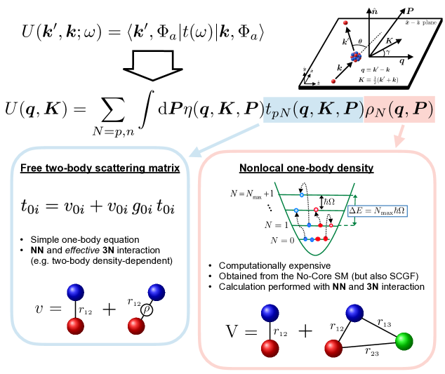
Figure 1: In this infographic the main building blocks of the optical potential are schematically shown along the main features of each components. For practical reasons the auxiliary optical potential $U$ is expressed as a function of the center-of-mass momentum ${\bm{K}}\equiv 1/2({\bm{k}}+{\bm{k}}^{\prime})$, and the momentum transfer ${\bm{q}}\equiv({\bm{k}}-{\bm{k}}^{\prime})$. It can be factorized into three pieces [13, 14, 15, 16]: the Möller correction $\eta({\bm{q}},{\bm{K}},{\bm{P}})$ that ensures the conservation of the transmitted flux after the transformation in the center-of-mass reference frame, the projectile-target potential $t_{NN}({\bm{q}},{\bm{K}};\omega)$ that depends also on the energy of the projectile $\omega$, and the structure component $\rho_{N}({\bm{q}},{\bm{P}})$, i.e. the Fourier transform of the non-local matter density in the momentum space. For both inputs we show into the coloured insertions the main features. For the potential part, at the moment, we are able to include the full $NN$ interaction and averaged $NNN$ contributions in terms of a medium density-dependent $NN$ interaction [17]. This solution requires to fix a density $\bar{\rho}$ at which the calculations are performed. So far [7, 8] we decided to explore the impact of $NNN$ terms performing calculations for several values of $\bar{\rho}$ (usually in the range $0.08$ fm${}^{-3}\leq\bar{\rho}\leq 0.13$ fm^-3, see Figs 1-6 of Ref. [7]). Investigations in this direction are currently underway [18]. For the structure part we used the NCSM [21] for light nuclei that allows us to fully use both $NN$ and $NNN$ terms (see Sect II and III. of Ref. [7]). For medium nuclei other approaches should be explored, like Self-Consistent Green Functions (SCGF) [22, 23].

Then, from a practical point of view, the OP can be computed in momentum space as follows (after some mathematical manipulations that can be found in Refs. [13, 14, 15, 16])

$$\begin{split}U({\bm{q}},{\bm{K}};E)=\sum_{N=p,n}&\int d{\bm{P}}\;\eta({\bm{q}},{\bm{K}},{\bm{P}})\,t_{NN}\left[{\bm{q}},\frac{1}{2}\left(\frac{A+1}{A}{\bm{K}}+\sqrt{\frac{A-1}{A}}{\bm{P}}\right);E\right]\\ &\times\rho_{N}\left({\bm{P}}+\sqrt{\frac{A-1}{A}}\frac{{\bm{q}}}{2},{\bm{P}}-\sqrt{\frac{A-1}{A}}\frac{{\bm{q}}}{2}\right)\,,\end{split}$$ (7)

where ${\bm{q}}$ and ${\bm{K}}$ represent the momentum transfer and the average momentum, respectively. Here ${\bm{P}}$ is an integration variable, $t_{NN}$ is the $NN$ $t$ matrix and $\rho_{N}$ is the one-body nuclear density matrix. The parameter $\eta$ is the Möller factor, that imposes the Lorentz invariance of the flux when we pass from the $NA$ to the $NN$ frame in which the $t$ matrices are evaluated. Finally, $E$ is the energy at which the $t$ matrices are evaluated and it is fixed at one half the kinetic energy of the incident nucleon in the laboratory frame.

As shown in Fig. 1, the calculation of Eq. (7) requires two external inputs: the $NN$ $t$ matrix and the one-body density $\rho_{N}$.

The calculation of the density matrix could be performed using different ab initio approaches. The method followed in Refs. [19, 20], where one-body translationally invariant densities were computed within the ab initio No-Core Shell Model (NCSM) [21] approach proved to be very successful in our own works [7, 9]. Alternatively other methods could be used, i.e. Self-Consistent Green Functions (SCGF) [22, 23], that allow to overcome the main limitation of the NCSM method, namely the severe limits on the atomic mass of the target nucleus due to the computational overload. Work in this direction is currently underway and a thorough investigation of nickel and calcium isotopes will soon appear [24]. For heavier nuclei, the only available method is Density Functional Theory (DFT). Even if most of the parametrizations have a phenomenological derivation, in recent years some authors [25] started to employ such approach from an ab initio point of view.

The main advantages of using ab initio methods in our framework is twofold. On one hand we can preserve the consistency of our theoretical framework if the same realistic interactions are used both for the structure part and the projectile-target interaction (with some caveats explained in Refs. [3, 5, 6, 8, 7]) and, on the other hand, we are able to provide more theoretically founded predictions for exotic nuclei since we do not have to rely on any fitting procedure on any selections of stable nuclei.

To calculate the projectile-target potential we rely on modern $NN$ potentials derived in the framework of Chiral Perturbation Theory (ChPT). Among the many available choices of realistic potentials, i.e. those that reproduce phase-shifts and binding energies of light nuclei with $\chi^{2}|_{\rm data}\simeq 1$, the choice of chiral potentials over phenomenological ones responds to some important requirements that will be listed shortly below.

Generally speaking, ChPT is a perturbative technique for the description of hadron scattering amplitudes based on expansions in powers of a parameter that can be generally defined as $(p,m_{\pi})/\Lambda_{b}$, where $p$ is the magnitude of three-momenta of the external particles, $m_{\pi}$ is the pion mass, and $\Lambda_{b}$ is the chiral symmetry breaking scale [26]. ChPT respects the low-energy symmetries of Quantum ChromoDynamics (QCD) and, up to a certain extent, is model independent and systematically improvable by an order-by-order expansion, with controlled uncertainties from neglected higher-order terms [27]. Both the fact that ChPT is directly connected to QCD and that the $NN$ components (and also $NNN$) are organized in terms of a systematic theoretical expansion is a huge improvement respect to conventional $NN$ potentials, like CD-Bonn [28] or Nijmegen [29]. The hierarchy of terms could also be exploited in order to provide an estimate for the theoretical uncertainties.

From a practical point of view, for our own calculations [3, 5, 6, 7, 8, 9] we mainly employed the $NN$ chiral interactions developed by Entem et al. [30, 31] up to the fifth order (N⁴LO) or, alternatively, the ones developed by Epelbaum et al. [32, 33] following a different strategy. The main difference between the two theoretical approaches of the chiral potentials concerns the renormalization procedures. The strategy followed in Refs. [32, 33] consists in a coordinate space regularization for the long-range contributions, and a conventional momentum space regularization for the contact (short-range) terms. On the other hand, for Refs. [30, 31], a slightly more conventional approach was pursued. A spectral function regularization was employed to regularize the loop contributions and a conventional regulator function to deal with divergences in the Lippman-Schwinger equation.

The three-nucleon forces deserve a separate treatment since so far we can employ genuine $3N$ forces only to compute the one-body densities of the target nuclei (up to the third order N²LO with a local and nonlocal regularization [34, 35]). At N²LO order we include the $2\pi$ exchange diagram between three nucleons, a one-$\pi$-exchange plus a $NN$ contact term and a $3N$ contact term. For more details and an explicit derivation of the relevant formulae, we refer the reader to Refs. [34]. For the projectile-target part we follow the prescriptions by Holt et al. [17] to derive a suitable density-dependent NN interaction.

2.1 A selection of results

To show the robustness of our proposed approach we will show a couple of non trivial calculations perfomed in the last years. The first case is the elastic proton scattering on ⁷Li, in which the target nucleus has spin and parity quantum numbers $J^{\pi}=3/2^{-}$. Theoretical predictions along with the experimental data are presented in Fig. 2.

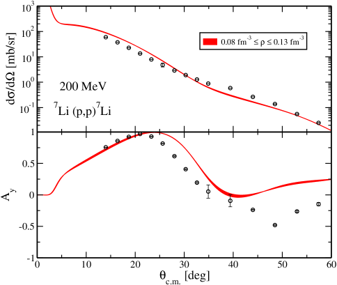
Figure 2: Differential cross section (upper panel) and analyzing power (lower panel), as functions of the center-of-mass scattering angle, for 200 MeV protons elastically scattered from ⁷Li (J^π = 3/2^-). The results were obtained using the $NN$ $t$ matrix computed with the $NN$ chiral interaction at N³LO order supplemented by a density dependent NN interaction (where the baryon density is varied in the range between 0.08 fm^-3 and 0.13 fm^-3) and the one-body nonlocal density matrices computed with the NCSM method using realistic nucleon-nucleon and three-nucleon local-nonlocal chiral interactions.

The differential cross section and analyzing power were measured at the Indiana University Cyclotron Facility using a polarized proton beam at a laboratory bombarding energy of 200.4 MeV [36]. The agreement between the theoretical prediction and the empirical data is good for the differential cross section, over all the angular distribution shown in the figure, and satisfactory for the analyzing power for values of the scattering angle up to $\sim 45^{\rm o}$.

The second test case is an extension much needed for future applications: inverse kinematics. In fact, in recent years, experimental efforts have multiplied to develop the technologies necessary to study the elastic scattering of protons (and ions) by using inverse kinematics. This configuration is necessary to study exotic nuclei that have very short average lifetimes. A very interesting experiment performed at the GSI was the study of the scattering of ^56,58Ni nuclei on hydrogen targets at energies near 400 MeV/nucleon in inverse kinematics for the determination of the distribution of nuclear matter [37]. Since the only theoretical approach used so far to analyze the experimental data is the Glauber model which contains phenomenological inputs, it is mandatory to establish a framework in which microscopic calculations could help understading experimental results.

In Fig. 3 we show the results only for $t\leq 0.1$ (GeV/c)² in the laboratory system because, due to the challenges of inverse kinematics, the regime of the elastic scattering needs to be focused at small center-of-mass angles. The agreement with experimental data is impressive despite the different kinematics and the high-energy regime at which the measurements are performed.

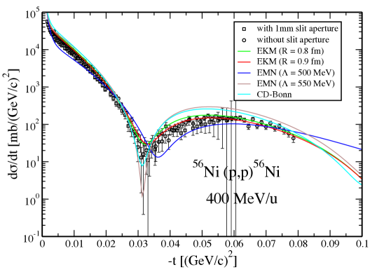
Figure 3: Differential cross section as a function of the Mandelstam variable $t$ in the laboratory frame for ⁵⁶Ni(p, p)⁵⁶Ni elastic scattering at $E=400$ MeV/u. Calculations are performed with different microscopic OPs derived from the $NN$ chiral potentials of Epelbaum et al. (EKM) [32, 33] and Entem et al. (EMN) [30, 31] at N⁴LO in comparison with the well known CD-Bonn [28]. With empty black squares and circles are shown the empirical data along with the corresponding error bars [37].

3 Necessary extensions

Among the different extensions under development, we would like to mention probably the most relevant one: the inclusion in our framework of inelastic reactions.

In the previous sections we mentioned a class of experiments that usually need the subtraction of contributions from the inelastic channel to perform a correct data analysis. In this perspective, if we wish to establish a consistent microscopic approach for inelastic NA scattering, which is our long-term goal, it is mandatory to develop a two-step theory program: first a reliable description of OPs for states with spin-parity quantum numbers J${}^{\pi}\neq 0^{+}$ (already under study with good results [7]) and then an extension of our formalism that, so far, is restricted to the elastic channel.

Let’s suppose to extend the definition of the projection operator $P$

$$P\equiv P_{0}+P_{1}=\ket{\Psi_{0}}\bra{\Psi_{0}}+\ket{\Psi_{1}}\bra{\Psi_{1}}\,,$$ (8)

with still $P+Q=\hbox{$1\hskip-1.2pt\vrule depth=0.0pt,height=6.88889pt,width=0.7pt\vrule depth=0.0pt,height=0.3pt,width=1.19995pt$}$. Inserting this relation into the many-body Lippmann-Schwinger equation we could follow the same prescriptions adopted for elastic case to define the following quantities

$$T_{00}\equiv P_{0}TP_{0}\,,\quad T_{01}\equiv P_{0}TP_{1}\,,\dots\quad G_{00}\equiv P_{0}G_{0}(E)P_{0}\,,\ldots$$ (9)

that represent the new scattering amplitudes that can be accomodated in a matrix form as follows (see Fig. 4)

$${\bm{T}}={\bm{U}}+{\bm{U}}{\bm{G}}{\bm{T}}\,,$$ (10)

with the previous terms defined as

$${\bm{T}}\equiv\begin{pmatrix}T_{00}&T_{01}\\ T_{10}&T_{11}\end{pmatrix}\,,\qquad{\bm{U}}\equiv\begin{pmatrix}U_{00}&U_{01}\\ U_{10}&U_{11}\end{pmatrix}\,,\qquad{\bm{G}}\equiv\begin{pmatrix}G_{00}&0\\ 0&G_{11}\end{pmatrix}\,.$$ (11)

When projected on the momentum basis, the equation for the $00$ component of the scattering matrix becomes

$$T_{00}({\bm{k}}^{\prime},{\bm{k}})=U_{00}({\bm{k}}^{\prime},{\bm{k}})+\int d{\bm{p}}\frac{U_{00}({\bm{k}}^{\prime},{\bm{p}})T_{00}({\bm{p}},{\bm{k}})}{E-E(p)+i\epsilon}+\int d{\bm{p}}\frac{U_{01}({\bm{k}}^{\prime},{\bm{p}})T_{10}({\bm{p}},{\bm{k}})}{E-E(p)-e_{1}+i\epsilon}\,,$$ (12)

and similarly for the other equations. Here $e_{1}$ is the excitation energy of the first excited state. Of course the previous equation has to be expanded in partial waves along with the other 3 equations. Work along this direction is in progress [38].

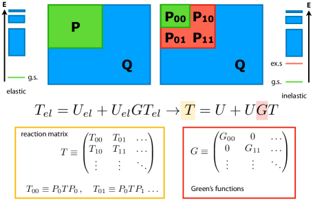
Figure 4: This infographic shows how the structure of Eq. 2 must change in order to include the description of inelastic processes. In order to accommodate the inclusion of the relevant excited state, it is necessary to calculate four optical potentials that describe all the available scattering channels. According to this picture we would need both stationary and transition densities.

References

References

- [1] Epelbaum E, Hammer H W and Meissner U G 2009 Rev. Mod. Phys. 81 1773
- [2] Machleidt R and Entem D R 2011 Phys. Rep. 503 1
- [3] Vorabbi M, Finelli P and Giusti C 2016 Phys. Rev. C 93 034619
- [4] Riesenfeld W B and Watson K M 1956 Phys. Rev. 102 1157
- [5] Vorabbi M, Finelli P and Giusti C 2017 Phys. Rev. C 96 044001
- [6] Vorabbi M, Finelli P and Giusti C 2018 Phys. Rev. C 98 064602
- [7] Vorabbi M, Gennari M, Finelli P, Giusti C, Navrátil P and Machleidt R 2022 Phys. Rev. C 105 014621
- [8] Vorabbi M, Gennari M, Finelli P, Giusti C, Navrátil P and Machleidt R 2021 Phys. Rev. C 103 024604
- [9] Vorabbi M, Gennari M, Finelli P, Giusti C and Navrátil P 2020 Phys. Rev. Lett. 124 162501
- [10] Castelvecchi D 2022 Nature 605 201
- [11] Hebborn C et al., arXiv:2210.07293 [nucl-th]
- [12] Chinn C R, Elster Ch, Thaler R M and Weppner S P 1992 Phys. Rev. C 52 1992
- [13] Elster Ch and Tandy P C 1989 Phys. Rev. C 40 81
- [14] Elster Ch, Cheon T, Redish E F and Tandy P C 1990 Phys. Rev. C 41 814
- [15] Elster Ch, Weppner S P and Chinn C R 1997 Phys. Rev. C 56 2080
- [16] Weppner S P, Elster Ch and Huber D 1998 Phys. Rev. C 57 1378
- [17] Holt J W, Kaiser N and Weise W 2010 Phys. Rev. C 81 024002
- [18] Vorabbi M, Finelli P and Giusti C, in preparation
- [19] Burrows M, Elster Ch, Popa G, Launey K, Nogga A and Maris P, 2017 Phys. Rev. C 97 024325
- [20] Gennari M, Vorabbi M, Calci A and Navrátil P 2017 Phys. Rev. C 97 034619
- [21] Barrett B R, Navrátil P and Vary J P 2013 Prog. Part. Nucl. Phys. 69 131
- [22] Dickhoff W H and Barbieri C 2004 Prog. in Part. and Nuc. Phys. 52 377
- [23] Carbone A, Cipollone A, Barbieri C, Rios A and Polls A 2013 Phys. Rev. C 88 054326
- [24] Vorabbi M, Barbieri C, Somà V, Finelli P and Giusti C, in preparation
- [25] Marino F, Barbieri C, Carbone A, Colò G, Lovato A, Pederiva F, Roca-Maza X and Vigezzi E, 2021 Phys. Rev. C 104 024315
- [26] Scherer S 2003 Adv. Nucl. Phys. 27 277
- [27] Georgi G 1993 Ann. Rev. Nucl. Part. Sci. 43 209
- [28] Machleidt R 2001 Phys. Rev. C 63 024001
- [29] de Swart J J, Klomp R A M M, Rentmeester M C M and Rijken T A, 1995 Few Body Syst. Suppl. 8 438
- [30] Entem D R, Kaiser N, Machleidt R and Nosyk Y 2015 Phys. Rev. C 91 014002
- [31] Entem D R, Machleidt R and Nosyk Y 2017 Phys. Rev. C 96 024004
- [32] Epelbaum E, Krebs H and Meißner U - G 2015 Phys. Rev. Lett. 115 122301
- [33] Epelbaum E, Krebs H and Meißner U - G 2015 Eur. Phys. J. A 51 53
- [34] Navràtil P 2007 Few-Body Syst. 41 117
- [35] Gysbers P, Hagen G, Holt J D, Jansen G R , Morris T D, Navrátil P, Papenbrock T, Quaglioni S, Schwenk A, Stroberg S R and Wendt K A 2019 Nat. Phys. 15 428
- [36] Glover C W, Foster C C, Schwandt P, Comfort J R, Rapaport J, Taddeucci T N, Wang D, Wagner G J, Seubert J, Carpenter A W, Carr J A, Petrovich F, Philpott R J and Threapleton M J 1991 Phys. Rev. C 43 1664
- [37] Von Schmid M 2015 Nuclear matter distribution of 56Ni measured with EXL, https://d-nb.info/1112044388/34, Ph. D. Thesis
- [38] Vorabbi M, Gennari M, Finelli P, Giusti C and Navrátil P, in preparation