Fast convolution kernels on pascal GPU with high memory efficiency

Abstract

The convolution computation is widely used in many fields, especially in CNNs. Because of the rapid growth of the training data in CNNs, GPUs have been used for the acceleration, and memory-efficient algorithms are focused because of thier high performance. In this paper, we propose two convolution kernels for single-channel convolution and multi-channel convolution respectively. Our two methods achieve high performance by hiding the access delay of the global memory efficiently, and achieving high ratio of floating point Fused Multiply-Add operations per fetched data from the global memory. In comparison to the latest Cudnn library developed by Nvidia aimed to accelerate the deep-learning computation, the average performance improvement by our research is 2.6X for the single-channel, and 1.4X for the multi-channel.

1 Introduction

Convolution is widely used as a fundamental operation in many applications such as computer vision, natural language processing, signal processing. Especially, the Convolution Neural Network (CNN), a popular model used for deep-learning, is widely used in many applications such as image recognition [2][6], video analysis[3], natural language processing[7], and has yielded remarkable results.

Recently, many CNN models have been proposed, such as AlexNet [15], GoogleNet [11], VGGNet [6], ResNet [9], etc. They are used in many areas, and are improved steadily. The sizes of their networks have grown larger, and this leads to the increase of their processing time. The CNNs have several layers, but a large portion of the total processing time is used for the convolution layers. Because of the high inherent parallelism of the convolution algorithms, many researchers are exploring to use GPUs to accelerate them. They can be divided into four categories: 1) Direct-based method, 2) FFT-based method, 3) Winograd-based method and 4) General matrix multiplication (GEMM) based method.

Recently, many of the algorithms and their modified versions have been aggregated into a public library called Cudnn by Nvidia, which aims to accelerate the deep-learning platforms like Chainer[4], Caffe[14], etc. As the volume of the processing data used in deep-learning increases, the memory-efficient algorithms play an increasingly more important role, resulting in the constant proposal of many improved versions. Among them, Implicit-GEMM[12] has been included in the Cudnn because of its high efficiency. It divides the feature map and the filter data into many sub-blocks and converts them to many sub-matrices by using only on-chip memory of GPU, not using global memory. This method is very memory-efficient, and achieved a high ratio of floating point Fused Multiply-Add (FMA) operations per data transferred from the global memory. In [1], two memory-efficient methods were proposed. Both of them are faster than the Implicit-GEMM, however their performances are negatively affected when the feature map size is smaller than 32, because it fixes the amount of the data assigned to each $SM$, which sometimes is not suitable to the small feature map. In CNN models such as [15][11][6][9], more than half of the convolution layers are used for the calculation of the images smaller than 32 (such as 28, 14, 7). This means that [1] cannot handle the modern CNN models efficiently.

In this paper, we propose two methods to accelerate the convolution kernels for single-channel and multi-channel respectively. In these methods, the memory access is optimized to achieve higher performance. For the single-channel kernel, our approach follows the computation method proposed in [1], however, the data are divided and assigned to each $SM$ carefully to hide the access delay of the global memory considering the input data size and the hardware features of our target GPUs (Pascal GPUs). For the multi-channel kernel, we propose a stride-fixed block method. This method aims to maximize the number of FMA operations per loaded data because the total amount of data that have to be loaded to each $SM$ is much larger than the single-channel convolution, and the access delay can be hidden by data prefetching.

2 Optimization Methods

In this section, we first introduce the CNN models, and then discuss what kind of optimization method is applicable on Pascal GPUs.

2.1 The Convolution Models

The multi-channel convolution can be defined as follows:

$$\begin{split}O^{m}(x,y)=\sum_{ch=1}^{C}\sum_{i=0}^{K-1}\sum_{j=0}^{K-1}I^{ch}(x+i,y+j)\cdot F^{ch,m}(i,j),\\ where\hskip 14.22636ptx\in[0,W_{x}-K+1),y\in[0,W_{y}-K+1),m\in[1,M].\end{split}$$ (1)

Here, $I$ is the input feature map set and $F$ is the input filter set. $O$ is the output feature map set which is generated from $I$ and $F$. $x$ and $y$ are the coordinates of the pixels of the feature maps. $W_{x}$ is the width and $W_{y}$ is the height of the input feature map. $i$ and $j$ are the offsets, and are added to the coordinates. Their upper bound $K$ decides the size of filter. $ch$ represents the channel of the input in the range of $[1,C]$ ($C$ is the number of channels), and all of the convolution results are added along the dimension $ch$. $m$ represents the filter number, and each filter has $C$ channels. $M$ is the number of filters, and it is defined in each convolution layer. When $C=1$, it is called single-channel convolution, and its definition is given the following equation.

$$\begin{split}O^{m}(x,y)=\sum_{i=0}^{K-1}\sum_{j=0}^{K-1}I(x+i,y+j)\cdot F^{m}(i,j)\\ \end{split}$$ (2)

2.2 Acceleration models on GPU

Here, we discuss the acceleration methods of the convolution calculation. However, this discussion is not restricted to the convolution, and can be applied to other applications.

In GPUs, the on-chip memory including registers and shared memory, and the off-chip memory, mainly the global memory are supported. The register is the fastest, and the global memory is the slowest and largest. To fully utilize this hierarchy, many studies such as [1] have been proposed. However, throughout all computation, data loading time from the global memory to the on-chip memory is most critical, and hiding the latency of the global memory is the most important point for the acceleration.

To hide the latency of the global memory, two methods can be considered:

1. keep the operation units busy (mainly Fused Multiply-Add (FMA) operation units in convolution) by executing more than $N_{FMA}$ operations (the lowest value to make the units busy) in each $SM$ for the current data set until the next data set arrive from the global memory by data prefetching, and

2. transfer a large volume of data ($V_{s}$) from the global memory continuously.

In most cases, the first approach is preferable, because the data loading overhead from the global memory can be relatively reduced more by executing more number of operations per loaded data. In the multi-channel convolution, the data size is large enough, and it is possible to find the division of the feature maps and filters that makes it possible to execute more than $N_{FMA}$ operations in each $SM$. However, in the single-channel convolution, when the size of feature maps is small, the number of executable operations becomes less than $N_{FMA}$ even with the data prefetching, and the second approach is required. Thus, it is necessary to make it clear under what conditions which method shows better performance.

Table 1 shows several parameters of GTX 1080Ti and its performance for accessing single precision data. As shown in Table 1, in GTX 1080Ti, 2 FMA operations can be executed in one clock cycle in each core, namely 256 FMA operations in each $SM$ (each $SM$ has $N_{cores}$ = 128 cores). According to the method proposed in [5], the global memory latency of the GTX 1080Ti is 258 clock cycles. In order to hide this 258 clock cycles, $N_{FMA}=66,048$ FMA operations ($66,048=258\times N_{cores}\times 2$) are required in each $SM$ for the current data set (the set of divided feature maps and filters).

The volume size $V_{s}$ can be calculated as follows. The Geforce GTX 1080Ti has a base clock of 1480 MHz and the bandwidth of 484 GB/s, which means the transfer rate is roughly 327 bytes per clock cycle. Therefore, the volume size which is needed to hide the latency (258 clock cycles) becomes 84,366 = 327 $\times$ 258 bytes. To realize the data transfer of this size, 21,120 ($=$ 84,366 / 4) threads are required because each thread fetches a 4 byte data in single precision. Thus, in each of 28 $SMs$ ($N_{sm}=28$ is the total number of $SMs$ in the GTX 1080Ti), 768 threads are required to fetch one 4-byte word respectively (in total, it becomes 768 $\times 4\times 28=$ 86,016 > 84,366). This means that the minimum volume size to make the global memory busy is $V_{s}=$ 86,016 bytes. For dividing the feature maps and filters, and assigning them to each $SM$, the following procedure should be taken:

1. Divide the feature maps and filters so that the total size of data that are assigned to each $SM$ is smaller than the size of the shared memory $S_{shared}$ (96KB in GTX 1080Ti).

2. Evaluate the number of FMA operations that can be executed for the data in each $SM$.

3. If it is larger than $N_{FMA}$, use the the first method which is based on the data prefetching.

4. If not, redivide the feature maps and filters so that the total size of data that are transferred to all $SMs$ becomes larger than $V_{s}$, and use the second approach.

Additionally, for accessing global memory, it is necessary to confirm that the starting address and the size of the sequential accessing segment is a multiple of 32-byte. In Pascal GPU, a multiple of 128-byte shows better performance than that of 32-byte and 64-byte, but the performance for 32-byte and 64-byte is acceptable.

Table 1: Parameters to access single precision data

	GTX 1080Ti
Architecture	Pascal
Global Memory Latency (clock cycles)	258
Bandwidth (Gb/s)	484
Base clock cycle (MHz)	1480
SM	28
Transmission Rate (Byte/clock cycle)	327
Data Requirement (bytes)	84,366
Thread Requirement/SM	768
Warp Requirement/SM	24
Data Requirement/SM (bytes)	3072
Flops/clock cycle/core	2

2.3 Data Mapping

As shown in Fig.1(a), in the single-channel convolution ($C=1$), the size of each filter is $K\times K\times{4\mbox{-}byte}$, and they are stored in the global memory continuously. With this data mapping, the filters can be divided only along the dimension $m$, and the filters can be loaded from the global memory efficiently because they are stored continuously. Three approaches for dividing the feature maps and filters can be considered.

1. Only the filters are divided. They are assigned to each $SM$, and in each $SM$, the assigned filters are applied to the whole feature maps (the feature map is processed sequentially against each filter).

2. Only the feature maps are divided. They are assigned to each $SM$, and in each $SM$, the assigned feature maps are processed by all filters (the filters are applied sequentially).

3. Both feature maps and filters are divided, and they are assigned to each $SM$ (the combination of the first and the second approach).

By using different approach, the amount of data that has to be loaded to the shared memory memory from the global memory, and the number of FMA operations that can be executed in parallel become different. Therefore, finding a good balance between the size of divided feature maps and filters becomes a key point.

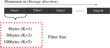
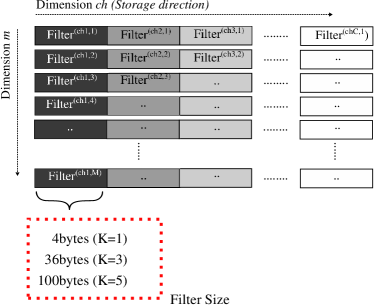
(a) Single-Channel (b) Multi-Channel

Figure 1: Memory storage form of the Filter

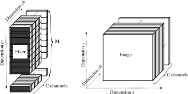
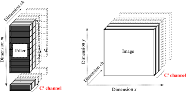
(a)       (b)

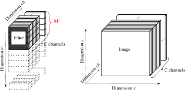
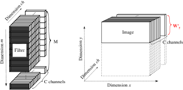
(c)       (d)

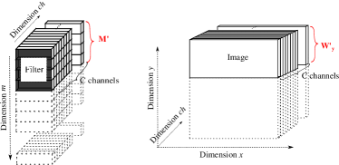
(e)

Figure 2: Assignment of the input data

In the multi-channel convolution ($C>1$), which is the typical case in the convolution layers of the CNN except for the first one, the data size becomes much larger than the single-channel convolution. Fig.1(b) shows how the filters are stored in the global memory. They are stored along the dimension $ch$ first, and then along the dimension $m$. In this case, the dividing method of the filters along the dimension $m$ as used for the single-channel convolution can not be applied as it is, because the data size of each filter is normally not a multiple of 32-byte. Especially when $K=1$ (the filter size is only 4 bytes), the filters are accessed as 4-byte segments, and it causes serious performance reduction because of non-coalescing memory access.To solve this problem, several approaches can be considered. Fig.2(a) shows the whole data structure before the data division.

1. In Fig.2(b), both the filters and the feature maps are divided along the dimension $ch$, and the data for $C^{\prime}=C/N_{sm}$ channels are assigned to each $SM$ ($N_{sm}$ is the total number of $SMs$). With this division, the data calculated in each thread have to be summed along dimension $ch$. This means that add operations among $SMs$ are required, and $W_{x}\times{W_{y}\times{C^{\prime}}\times{4\mbox{-}byte}}$ byte in the global memory are used for this summation. The global memory accesses to this area and the synchronous operations required for this summation considerably reduce the overall performance.

2. In Fig.2(c), only the filters are divided along the dimension $m$. $M^{\prime}\times C=M/N_{sm}\times C$ filters are assigned to each $SM$, and the whole feature map are loaded to $SMs$ from the global memory. In this approach, if the total size of the filters is less than the total size of all shared memory ($K\times K\times C\times M\times 4\mbox{-}byte<N_{sm}\times S_{shared}$), the divided filters can be cached in each $SM$, and no additional access to the global memory is required.

3. On the other hand, in Fig.2(d), only the feature maps are divided along dimension $y$. The divided feature maps are assigned to each $SM$, and the whole filters are loaded to $SMs$ from the global memory. In this case, if the total size of the feature maps is smaller than the total size of the shared memory, the divided feature maps can be cached in each $SM$, and no additional access to the global memory is required.

4. However, the total size of the filters and feature maps are larger than the total size of the shared memory in general. Thus, as shown in Fig.2(e), both the filters and feature maps have to be divided respectively, and each divided segments is cached in each $SM$ or loaded from the global memory. In this case, there exist many alternatives for how to divide the filters and features maps.

According to our preliminary evaluation, the performance with the data dividing method along the dimension $ch$ (Fig.2(b)) is obviously slower than other dividing methods because of the additional access to the global memory for the addition. For achieving higher performance, it is necessary to choose other dividing methods considering the data size and the hardware features of the target GPUs so that in each $SM$ the number of FMA operations that can be executed per loaded data from the global memory is maximized.

3 GPU Implementation

According to the discussion in Section 2, in both the single-channel and multi-channel convolution, it is important to make the number of FMA operations per pre-fetched data higher than $N_{FMA}$ in order to achieve higher performance. However, in some cases of the single-channel convolution, for example when the size of feature maps is small, the number of FMA operations cannot be kept high enough by data prefetching. This means that, in case of single channel convolution, according to the size of input data, we need to choose one of the two methods described in Section 2.2: data prefetching or data transfer larger than $V_{s}$.

In the multi-channel convolution, the size of input data is large enough, and the number of FMA operations can be kept high enough by data prefetching. However, the performance can be improved more by achieving higher FMA operation ratio for the fetched data, because to fetch the data from the global memory, each thread has to issue the instruction to read data, and the clock cycles are spent for issuing these read instructions. Therefore, in the multi-channel convolution, to find the data dividing method that maximizes the number of FMA operations for each divided data is the key to achieve higher performance.

3.1 Single-Channel Convolution

Here, we describe how to divide the input data to achieve higher performance in the single channel convolution. As for the convolution calculation in each $SM$, we follow the method proposed in [1].

As shown in equation (4), the total amount of the input data is given by:

$$\begin{split}D_{input}=D_{filter}+D_{map}=(K\times{K}\times{M}+W_{x}\times{W_{y}})\times{4}\,Bytes.\end{split}$$ (3)

Let $N_{sm}$ be the number of $SMs$. There are two ways to divide the input data and assign them to each $SM$. In the first method, the input data is divided along the dimension $m$ of the filter. $D_{1}$, the size of input data assigned to each $SM$, becomes

$$\begin{split}D_{1}=\frac{D_{filter}}{N_{sm}}+D_{map}=(K\times{K}\times{\lceil\frac{M}{N_{sm}}\rceil}+W_{x}\times{W_{y}})\times{4}\,Bytes\end{split}$$ (4)

In general, $D_{map}$ is too large to be stored in the on-chip memory of each $SM$. Thus, $D_{map}$ is divided into $P$ pieces along the dimension $y$. The size of each piece becomes $D_{Inc1}=D_{map}/{P}$. Here, for each line of feature map, since the convolution requires additional $K-1$ lines, the amount of data that have to be held in the on-chip memory becomes

$$\begin{split}D_{1}=\frac{D_{filter}}{N_{sm}}+D_{Inc1}+(K-1)*W_{x}=(K\times{K}\times{\lceil\frac{M}{N_{sm}}\rceil}+(\lceil\frac{W_{y}}{P}\rceil+K-1)\times{W_{x}})\times{4}\,Bytes\end{split}$$ (5)

and the number of FMA operation that can be executed for these data in each $SM$ is given by

$$\begin{split}Th_{1}=\frac{D_{filter}}{N_{sm}}\times{D_{Inc1}}=K\times{K}\times{\lceil\frac{M}{N_{sm}}\rceil}\times{\lceil\frac{W_{y}}{P}\rceil\times{W_{x}}}.\end{split}$$ (6)

In the second method, the input data is divided along the dimension $y$ of the feature map. In this case, $D_{2}$, the amount of the input data assigned to each $SM$, becomes

$$\begin{split}D_{2}=D_{filter}+\frac{D_{map}}{N_{sm}}=(K\times{K}\times{M}+({\lceil\frac{W_{y}}{N_{sm}}\rceil+K-1})\times{W_{x}})\times{4}\,Bytes.\end{split}$$ (7)

$D_{filter}$ is too large to be stored in the on-chip memory in general, and it is divided into $Q$ pieces. The size of each piece becomes $D_{Inc2}=D_{filter}/{Q}$. Then, $D_{2}$ becomes

$$\begin{split}D_{2}=D_{Inc2}+\frac{D_{map}}{N_{sm}}=\frac{D_{filter}}{Q}+\frac{D_{map}}{N_{sm}}=(K\times{K}\times{\lceil\frac{M}{Q}\rceil}+(\lceil\frac{W_{y}}{N_{sm}}\rceil+K-1)\times{W_{x}})\times{4}\,Bytes\end{split}$$ (8)

and the number of FMA operation that can be executed for these data in each $SM$ is given by

$$\begin{split}Th_{2}=D_{Inc2}\times\frac{D_{map}}{N_{sm}}=K\times{K}\times{\lceil\frac{M}{Q}\rceil}\times({\lceil\frac{W_{y}}{N_{sm}}\rceil})\times{W_{x}}.\end{split}$$ (9)

The values of $P$ and $Q$ are decided considering if $D_{1}$ or $D_{2}$ is smaller than $S_{shared}$, and if $Th_{1}$ or $Th_{2}$ is larger than $N_{FMA}$. If $P=1$ or $Q=1$, the feature maps or the filters are not divided, and they are transferred to the on-chip memory at a time. If $P>1$ or $Q>1$, the feature maps or the filters are divided into several pieces, and the pieces are transferred to each $SM$ by using the data prefetching. With smaller $P$ and $Q$, $D_{1}$, $D_{2}$ and $Th_{1}$, $Th_{2}$ become larger. The lower bound of $P$ and $Q$ is given by the requirement that $D_{1}$ and $D_{2}$ have to be smaller than $S_{shared}$, and the upper bound is given by the requirement that $Th_{1}$ and $Th_{2}$ should be larger than $N_{FMA}$. $P$ and $Q$ should be chosen so that these requirements can be satisfied. In our implementation, $P$ and $Q$ are decided as follows.

1. $Th_{1}$ or $Th_{2}$ should be larger than the number of FMA operation $N_{FMA}$.
        $Th_{1}\geq N_{FMA}$ and $Th_{2}\geq N_{FMA}$
   Thus, the upper bound of $P$ and $Q$ (they must be smaller than $W_{y}$ and $M$ respectively) is given as follows
     $P\leq\frac{K\times{K}\times{\lceil\frac{M}{N_{sm}}\rceil}\times{W_{y}}\times{W_{x}}}{N_{FMA}}\,and\,P\leq{W_{y}}$,         $Q\leq\frac{K\times{K}\times{M}\times{\lceil\frac{W_{y}}{N_{sm}}\rceil}\times{W_{x}}}{N_{FMA}}\,and\,Q\leq{M}$

2. $D_{1}$ and $D_{2}$ must be smaller than the size of on-chip memory. The lower bound of $P$ and $Q$ is given as follows.
      $P\geq\frac{4\times{W_{y}}\times{W_{x}}}{S_{shared}-4\times{K\times{K\times{\lceil\frac{M}{N_{SM}}}\rceil}}+(1-K)\times{4}\times{W_{x}}}$,      $Q\geq\frac{4\times{M}\times{K}\times{K}}{S_{shared}-4\times{W_{x}}\times{(\lceil\frac{W_{y}}{N_{SM}}+K-1)}}$
   Actually, there exist one more requirement to decide this lower bound. The number of required registers for the computation must be smaller than that supported in each $SM$. Its detail is not shown here, but considering this requirement, the lower bound is calculated.

3. If there exist $P$ and $Q$ ($P$ and $Q$ must be an integer) in the range specified by (2) and (3), Any of them can be used. In our current implementation, the minimum ones are chosen as $P$ and $Q$, because the smaller values means less number of division, and make the processing sequence simpler. If no value exists, $P$ and $Q$ are set to 1.

4. Using the obtained $P$ and $Q$, $D_{1}$ and $D_{2}$ are calculated and compared. If $D_{1}$ is smaller than $D_{2}$, $Q$ is reset to 1 to use the first dividing method described above, and otherwise, $P$ is reset to 1 to use the second one. Both methods can be used because they both satisfy the requirements, but for the safety (for leaving more memory space on the on-chip memory), the smaller one is chosen.

Following this procedure, the input data are divided and allocated to each $SM$ in the best balance.

3.2 Multi-Channel Convolution

As described above, in the multi-channel convolution, both feature maps and filters are divided, and prefetching is used to transfer them to each $SM$ from the global memory. Recently, the block-based methods show high performance in convolution due to their continuous and simple memory access sequence. Fig.3 shows the data mapping of the filters and feature map, and how they are divided and calculated in each $SM$. In the block-based method, as shown in Fig.3(a), the following data are loaded to the on-chip memory in each $SM$.

1. $S$ bytes of each filter along the dimension $ch$ (called segment in the following discussion) of $M^{\prime}$ filters ($S\times{M^{\prime}}$ bytes in total), and

2. a part of feature map, $W^{\prime}_{x}\times{W^{\prime}_{y}}\times{4\,bytes}$ in the same channel ($W^{\prime}_{x}$ is an arbitrary value that is decided by the size of on-chip memory, but $W^{\prime}_{y}$ is specified as $\lceil\frac{S}{K\times{4bytes}}\rceil$, because when $S$ bytes are fetched along the dimension $ch$, $\lceil\frac{S}{K\times{4bytes}}\rceil$ lines in the feature map are required to apply the filter).

Then, the convolution is calculated for these data, and the next data (next $S\times M^{\prime}$ bytes of filters and $W^{\prime}_{y}\times W^{\prime}_{x}$ bytes of feature maps are loaded by data prefetching. In [1], the filter size is chosen as $S$ ($S=K\times{K}\times{4\,bytes}$), and only the filters of the target channel and a part of feature map of the same $channel$ are loaded to the on-chip memory. However, the filter size $K\times K$ is usually odd and often small, and the performance is seriously degraded because of non-coalescing memory access. [16] tried to solve this problem by extending $S$ to 128-bytes. By fetching continuous 128 bytes on the global memory, the highest memory throughput can be achieved in GPUs. In this method, the filters of several channels (and a part of the next channel) are fetched at the same time, and they are kept in the on-chip memory. First, only the filters of the first channel are used for the computation, and then, the filters of the next channel are used. With this larger $S$, $M^{\prime}$ has to be kept small because of the limited size of on-chip memory, and smaller $M^{\prime}$ means less parallelism ($M^{\prime}$ filters are applied in parallel to the feature map of the same channel). In [1], higher parallelism comes first, while in [16], lower access delay has a higher priority.

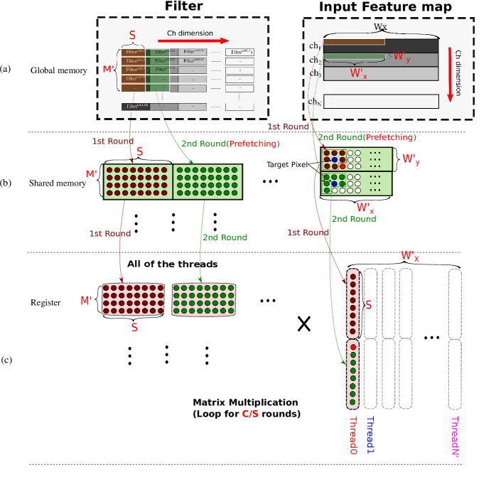
Figure 3: Multi-Channel Convolution Kernel

Here, we propose a stride-fixed block method not only to maintain the efficient global memory access, but also to achieve high parallelism in each $SM$.

1. $S$ is set to a multiple of 32-bytes. Actually, 32 or 64 is used. Small $S$ allows larger $M^{\prime}$, namely higher parallelism, under the limited size of on-chip memory. When $S$ is 32 or 64 bytes, the memory throughput from the global memory becomes a bit worse than $S=128$ bytes (the highest throughput), but it is acceptable. $S=32$ is the minimum value to maintain efficient global memory access.

2. Next, we fix $W^{\prime}_{x}$. $W^{\prime}_{x}$ pixels in the feature map are fetched along the dimension $x$ from the global memory. Thus, $W^{\prime}_{x}$ should be a multiple of 128-bytes to achieve the highest memory throughput. Larger $W^{\prime}_{x}$ is preferable because it increases the Instruction Level Parallelism (ILP), which can improve the performance of the convolution.

3. After deciding the values of $S$ and $W^{\prime}_{x}$, the most suitable $M^{\prime}$ can be found by the requirements of the number of FMA operations.
     $M^{\prime}\geq\frac{N_{FMA}\times{4\mbox{-}bytes}}{S\times{W^{\prime}_{x}}}$.

4. Because the data prefetching is used to fetch the next data set while the current data set is being used for the current calculation, the size of data set cannot exceeds the half of the size of shared memory. Thus,   $(S\times{M^{\prime}}+\lceil\frac{S}{K\times{4bytes}}\rceil\times{W^{\prime}_{x}})\leq\frac{S_{shared}}{2}$
   Here, $\lceil\frac{S}{K\times{4bytes}}\rceil=W^{\prime}_{y}$ is the number of feature maps required for the calculation.

With this approach, for given $S$, $W^{\prime}_{x}$ and $M^{\prime}$ to achieve high performance based on block method can be obtained.

From here, we describe how the convolution calculation is executed in each $SM$. As shown in Fig.3(a)(b), first, each $SM$ loads $S\,bytes$ of $M^{\prime}$ filters to the shared memory. At the same time, $W^{\prime}_{x}$ pixels on $\lceil\frac{S}{K\times{4bytes}}\rceil=W^{\prime}_{y}$ lines of the feature maps are also loaded. After the first round loading of these data, the same size of data for the next round are pre-fetched: the next $S\times M^{\prime}$ bytes along the dimension $ch$, and the next $W^{\prime}_{x}$ pixels of the $W^{\prime}_{y}$ lines. During the second round loading, the convolutions for the first round data set are calculated on the chip as shown in Fig.3(b)(c). On the chip, each thread corresponds to one target pixel of the feature map as shown in Fig.3(b). Because the accessing speed of registers is faster than that of shared memory, it is required to transfer each data in the shared memory to the registers in order to achieve high performance. In the convolution computation, the target pixel and its neighbors in the feature map are sent to the corresponding registers by each thread. Here, one important point is that only $S/{4bytes}$ pixels in the feature map have to be loaded onto the registers. The rest pixels, the red ones in Fig.3(b), are just held in the shared memory for the next round. The filter data are also transferred to the registers by the corresponding thread, but in this case, all data are transferred to the registers because all of them are used. After that, each pixel data is multiplied by the corresponding filter data, and their products are added. When all computations for the data stored in on-chip memory has been finished, data prefetching for the third round is started. During this loading, the convolution for the second round data is calculated.

By using this method, the size of $S$ can be kept small, and the number of filters $M^{\prime}$ can be increased. This ensures that more filters can be applied in parallel to the same feature map. This does not increase the number of data loading of the feature maps, and hides the latency caused by global memory access.

4 Experimental analysis

We implemented our two convolution kernels on Pascal series GPU Geforce GTX 1080Ti by using the CUDA 8.0. Their performances were evaluated using many convolutions which are commonly used in popular CNN models[15][9][6][11], and compared with the latest public library Cudnn v7.1[12].

In the single-channel convolution, we changed the sample size of the feature maps from 28 to 1K and the size of the corresponding channels from 512 to 32. The filter size is 1, 3 or 5, which is usually used in many CNN models. In CUDA programming, by assigning more number of blocks to each $SM$, the $SMs$ can be kept busy. In our current implementation, $N_{block}=2\times{N_{SM}}=2\times{28}$ blocks are used. Two blocks are assigned to each $SM$, and 512 threads are assigned to each block. Thus, the maximum number of registers for each thread is constrained to 128. For each tested case, $P$ and $Q$ are decided following the method described in Section 3.1. Fig.5 shows the results of the single-channel convolution. Our method is faster than Cudnn v7.1 in all tested cases. The performance gain is 1.5X to 5.6X, and its average is 2.6X. In the multi-channel convolution, we changed the sample size of the feature maps from 7 to 512, and the size of the corresponding channels from 64 to 512. The filter size is also 1, 3, or 5. As discussed in Section 3.2, larger $M^{\prime}$ is preferable for making data prefetching more effective. Therefore, we fixed the segment size $S$ as 32 or 64 bytes, and then $M^{\prime}$ and $W^{\prime}_{x}$ are decided following the method described in Section 3.2. According to our preliminary evaluation, when $M^{\prime}=64$ and $W^{\prime}_{x}=128$, the performance becomes best, and we used these values for this comparison. As shown in Fig.5, our method is faster than Cudnn in all tested cases, and the throughput has been increased by 1.05X to 2X, with an average increase of 1.39X. In [1], a different GPU is used, and a direct comparision is not possible. However, when $K=3$, our performance is 4X faster than [1] on GPU the peak performance of which is 2.4X faster than that used in [1].

We also implemented our two kernels on Maxwell series GPU GTX Titan X, and it also showed that our performance is faster than Cudnn on the same GPU by 1.3X to 3.7X in the single-channel convolution and 1.08X to 1.8X in the multi-channel convolution.

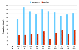
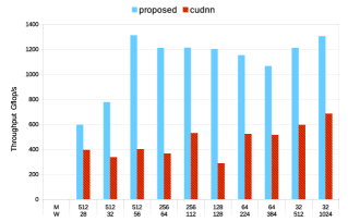
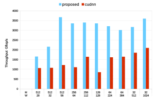
Filter Size = 1 Filter Size = 3 Filter Size = 5

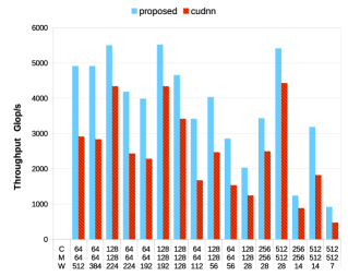
Figure 4: Performance of the Single-Channel Convolution Kernel

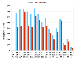
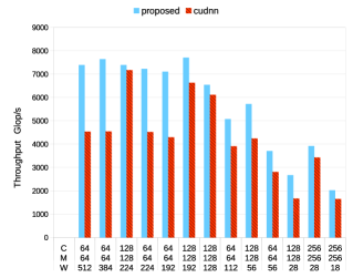
Filter Size = 1 Filter Size = 3 Filter Size = 5

Figure 5: Performance of the Multi-Channel Convolution Kernel

5 CONCLUSIONS

In this paper, we proposed two convolution kernels on Pascal series GPUs for single-channel and multi-channel respectively. For single-channel convolution, we introduced an effective method of data mapping, which can hide the access delay of the global memory efficiently. For multi-channel convolution, we introduced a method that not only guarantees the memory access efficiency, but also achieves high FMA operation ratio per loaded data. Performance comparison with the public library Cudnn shows that our approaches are faster in all tested cases: 1.5X to 5.5X in the single-channel convolution and 1.05X to 2X in the multi-channel convolution. Our approaches was designed assuming Pascal architecture, but the performance is also faster than Cudnn on Maxwell architecture. This practice shows that our approaches can be applied to the wide range of CNN models on various GPUs. In our current implementation, the throughput is still lower than the theoretical maximum. It means that the convolution kernel still has the room for improvement, and this is our main future work.

References

- [1] Xiaoming Chen, Jianxu Chen, Danny Z. Chen, Xiaobo Sharon Hu. “Optimizing Memory Efficiency for Convolution Kernels on Kepler GPUs,”In DAC, 2017.
- [2] A. Poznanski, L. Wolf, “Cnn-n-gram for handwriting word recognition,”in: CVPR, pp. 2305-2314, 2016.
- [3] D. Yu, W. Xiong, J. Droppo, A. Stolcke, G. Ye, J. Li, and G. Zweig, “Deep convolutional neural networks with layer-wise context expansion and attention,”in Proc.Interspeech, 2016.
- [4] Eddie Bell. “A implementation of squeezenet in chainer.”https://github.com/ejlb/squeezenet-chainer, 2016.
- [5] X. Mei, X. Chu, “Dissecting GPU memory hierarchy through microbenchmarking,”IEEE Trans. Parallel Distrib. Syst, 2016.
- [6] K. Simonyan and A. Zisserman. “Very deep convolutional networks for large-scale image recognition,”In ICLR, 2015.
- [7] Zhang, Y. and Wallace, B. “A sensitivity analysis of (and practitioners guide to) convolutional neural networks for sentence classification.”arXiv:1510.03820, 2015.
- [8] A. Lavin. “Fast algorithms for convolutional neural networks.”arXiv:1509.09308, 2015.
- [9] K. He, X. Zhang, et al. “Deep residual learning for image recognition,”arXiv:1512.03385, 2015.
- [10] S. Li, Y. Zhang, C. Xiang, and L. Shi. “Fast Convolution Operations on Many-Core Architectures.”In HPCC, pages 316-323, 2015.
- [11] Szegedy, C. et al. “Going deeper with convolutions.”Preprint at http://arxiv.org/abs/1409.4842, 2014.
- [12] Sharan Chetlur, Cliff Woolley, et al. “cuDNN: Efficient primitives for deep learning.”arXiv:1410.0759, 2014.
- [13] M. Mathieu, M. Henaff, et al. “Fast training of convolutional networks through ffts.”In CoRR, 2013.
- [14] Jia, Y. “Caffe: An open source convolutional architecture for fast feature embedding.” http://caffe.berkeleyvision.org/, 2013.
- [15] Krizhevsky, A., Sutskever, I., and Hinton, G. E. “ImageNet classification with deep convolutional neural networks,”In NIPS, pp. 1106-1114, 2012.
- [16] Guangming Tan, Linchuan Li, et al. “Fast implementation of DGEMM on Fermi GPU.”In Supercomputing 2011, pages 35:15:11, New York, NY, USA, 2011. ACM.
- [17] R. Nath, S. Tomov, and J. Dongarra. “An improved magma gemm for fermi gpus.”Technical Report 227, LAPACK Working Note, 2010.