Distributed Model Predictive Covariance Steering

Abstract

This paper proposes Distributed Model Predictive Covariance Steering (DMPCS), a novel method for safe multi-robot control under uncertainty. The scope of our approach is to blend covariance steering theory, distributed optimization and model predictive control (MPC) into a single methodology that is safe, scalable and decentralized. Initially, we pose a problem formulation that uses the Wasserstein distance to steer the state distributions of a multi-robot team to desired targets, and probabilistic constraints to ensure safety. We then transform this problem into a finite-dimensional optimization one by utilizing a disturbance feedback policy parametrization for covariance steering and a tractable approximation of the safety constraints. To solve the latter problem, we derive a decentralized consensus-based algorithm using the Alternating Direction Method of Multipliers (ADMM). This method is then extended to a receding horizon form, which yields the proposed DMPCS algorithm. Simulation experiments on large-scale problems with up to hundreds of robots successfully demonstrate the effectiveness and scalability of DMPCS. Its superior capability in achieving safety is also highlighted through a comparison against a standard stochastic MPC approach. A video with all simulation experiments is available here.

I Introduction

Multi-robot control is a domain with a significant variety of applications such as swarm robotics [1], multi-UAV navigation [2], motion planning [3], underwater vehicles [4], and so forth. As the scale and complexity of such systems continuously increases, some of the most desired attributes for algorithms designed to control these systems include safety under uncertainty, scalability and decentralization.

Model predictive control (MPC) has found several successful multi-robot applications [5, 6, 7], thanks to its optimization-based nature and intrinsic feedback capabilities. In the case where stochastic disturbances are present, several stochastic MPC (SMPC) approaches have been proposed for handling them such as [8, 9, 10, 11]. Nevertheless, the literature in combining MPC with the steering of the state distribution of a system to exact targets for enhancing safety remains quite scarce [12, 13, 14].

Covariance steering (CS) theory considers a class of stochastic optimal control problems, where the main objective is to steer the state mean and covariance of a system to desired targets. While initial CS approaches had dealt with infinite-horizon problems for linear time-invariant systems [15, 16], finite-horizon CS methods that also address linear time-variant dynamics, have recently gained attention such as [17, 18, 19, 20]. Several successful robotics applications of CS can be found in motion planning [21], trajectory optimization [13, 14], multi-agent control [22], etc.

In SMPC based methods, it is typically the feed-forward control inputs that are treated as optimization variables, while the feedback gains are fixed to a stabilizing value for the closed-loop system [9]. However, the state covariance cannot actively be steered with such methods, while fixed static feedback gains might perform poorly for time-varying dynamics. Thus, control policies resulting from standard SMPC approaches might be suboptimal and/or overly conservative against safety criteria. On the contrary, CS methods yield the optimal feedback gains that steer the state covariance to the desired targets, thus providing more flexibility to satisfy optimality and safety guarantees at the same time.

Although CS allows for finding the optimal control policies to steer the state statistics to desired values in the unconstrained case, the latter might be unreachable in the presence of state and/or input constraints. In MPC applications, especially, such infeasibilities can occur quite frequently, since the prediction horizon is usually much smaller than the total time horizon. Therefore, it would be desirable to penalize the deviation from the desired state statistics by utilizing a distance metric between distributions such as the Wasserstein distance [23], instead of imposing hard constraints [12].

In addition, the main limitation of applying CS methods to large-scale multi-robot systems lies in the fact that computational demands increase significantly with respect to the state/control dimension and time horizon. Nevertheless, recent work [22] has shown that this computational burden can be significantly alleviated by merging CS with the Alternating Direction Method of Multipliers (ADMM), an optimization procedure that has found several recent applications in decentralized control [24, 25, 26, 27].

In this paper, we propose Distributed Model Predictive Covariance Steering (DMPCS) for safe and scalable multi-robot navigation. First, we provide a problem formulation which utilizes the Wasserstein distance for steering the robots to prescribed target distributions and probabilistic constraints for ensuring their safe operation. Subsequently, by exploiting CS theory, a suitable disturbance feedback policy parametrization, and an efficient approximation of the safety constraints, we transform the original problem into a finite-dimensional optimization one. To solve this, we propose an ADMM-based method for establishing consensus between neighboring robots and achieving decentralization. The latter method is then integrated into an MPC scheme, which yields the final DMPCS algorithm. Simulation experiments on large-scale navigation tasks with up to hundreds of robots illustrate the efficacy and scalability of DMPCS. In addition, a comparison against a standard SMPC approach underlines the advantages of DMPCS in steering the distributions of the robots and achieving safety throughout the tasks.

II Problem Description

II-A Notation

The space of $n\times n$ symmetric, positive semi-definite (definite) matrices is denoted with $\mathbb{S}_{n}^{+}$ ($\mathbb{S}_{n}^{++}$). The $n\times n$ identity matrix is denoted as $I_{n}$ whereas $\mathbf{0}$ denotes the zero matrix (or vector) with appropriate dimensions. The trace operator is denoted with ${\mathrm{tr}}(\cdot)$. The expectation and covariance of a random variable (r.v.) $x\in\mathbb{R}^{n}$ are given by $\mathbb{E}[x]\in\mathbb{R}^{n}$ and ${\mathrm{Cov}}[x]\in\mathbb{S}^{+}_{n}$, respectively. With $x\sim\pazocal{N}(\mu,\Sigma)\in\mathbb{R}^{n}$, we refer to a Gaussian r.v. $x$ with $\mathbb{E}[x]=\mu$ and ${\mathrm{Cov}}[x]=\Sigma$. With $\llbracket a,b\rrbracket$, we denote the integer set $[a,b]\cap\mathbb{Z}$ for any $a,b\in\mathbb{R}$.. The cardinality of a set $\pazocal{X}$ is denoted with $|\pazocal{X}|$. Finally, given a set $\pazocal{C}$, we denote with $\pazocal{I}_{\pazocal{C}}(x)$ the indicator function such that $\pazocal{I}_{\pazocal{C}}(x)=0$ if $x\in\pazocal{C}$ and $\pazocal{I}_{\pazocal{C}}(x)=+\infty$, otherwise.

II-B Problem Description

Let us consider a team of $N$ robots given by the set $\pazocal{V}=\{1,\dots,N\}$. Each robot $i\in\pazocal{V}$ is subject to the following discrete-time, stochastic, nonlinear dynamics

$$x_{i,k+1}=f_{i}(x_{i,k},u_{i,k})+w_{i,k},\quad x_{i,0}\sim\pazocal{N}_{i,0},$$ (1)

for $k\in\llbracket 0,K\rrbracket$, where $K$ is the time horizon, $x_{i,k}\in\mathbb{R}^{n_{i}}$, $u_{i,k}\in\mathbb{R}^{m_{i}}$ and $f_{i}:\mathbb{R}^{n_{i}\times m_{i}}\rightarrow\mathbb{R}^{n_{i}}$ are the state, control input and transition dynamics function of the $i$-th robot, and $w_{i,k}\sim\pazocal{N}(0,W_{i})\in\mathbb{R}^{n_{i}}$ is zero mean Gaussian noise with $W\in\mathbb{S}_{n_{i}}^{+}$. Each robot’s initial state $x_{i,0}$ is given by a multivariate Gaussian distribution $\pazocal{N}_{i,0}=\pazocal{N}(\mu_{i,0},\Sigma_{i,0})$ with $\mu_{i,0}\in\mathbb{R}^{n_{i}}$ and $\Sigma_{i,0}\in\mathbb{S}_{n_{i}}^{+}$. The position of the $i$-th robot in 2D (or 3D) space is denoted with $p_{i,k}\in\mathbb{R}^{q}$ with $q=2$ (or $q=3$) and can be extracted with $p_{i,k}=H_{i}x_{i,k}$, where $H_{i}\in\mathbb{R}^{q\times n_{i}}$ is defined accordingly. Furthermore, the environment, wherein the robots operate, includes circle (in 2D) or spherical (in 3D) obstacles given by the set $\pazocal{O}=\{1,\dots,O\}$, where each obstacle $o\in\pazocal{O}$ has position $p_{o}\in\mathbb{R}^{q}$ and radius $r_{o}\in\mathbb{R}$.

We consider the problem of steering the state distributions of all robots $i\in\pazocal{V}$ to the target Gaussian ones $\pazocal{N}_{i,\mathrm{f}}=\pazocal{N}(\mu_{i,\mathrm{f}},\Sigma_{i,\mathrm{f}})$ with $\mu_{i,\mathrm{f}}\in\mathbb{R}^{n_{i}}$, $\Sigma_{i,\mathrm{f}}\in\mathbb{S}_{n_{i}}^{++}$. To penalize the deviation of the actual distributions from the target ones, we utilize the notion of the Wasserstein distance as a metric to describe similarity between r.v. probability distributions [23]. In particular, we define the following cost:

$$J_{i}:=\sum_{k=1}^{K}\pazocal{W}_{2}^{2}(x_{i,k},x_{i,\mathrm{f}})+\sum_{k=0}^{K-1}l_{i}(u_{i,k}),$$ (2)

for each robot $i\in\pazocal{V}$, where $x_{i,\mathrm{f}}\sim\pazocal{N}_{i,\mathrm{f}}$, $\pazocal{W}_{2}^{2}(x_{a},x_{b})$ is the squared Wasserstein distance between $x_{a},x_{b}$ and $l_{i}(u_{i,k})=u_{i,k}^{\mathrm{T}}R_{i}u_{i,k}$ penalizes the control effort with $R_{i}\in\mathbb{S}_{m_{i}}^{++}$.

The following probabilistic collision avoidance constraints between the robots and the obstacles are also imposed

$$\mathbb{P}(\|p_{i,k}-p_{o}\|_{2}\geq d_{i,o}+r_{o})\geq 1-\alpha,$$

$$\qquad\forall\ k\in\llbracket 0,K\rrbracket,\ i\in\pazocal{V},\ o\in\pazocal{O},$$ (3)

where $\alpha<0.5$ and $d_{i,o}\in\mathbb{R}$ is the minimum allowed distance between the center of robot $i$ and obstacle $o$. In addition, we also wish for all robots to avoid collisions with each other, through the following constraints

$$\mathbb{P}(\|p_{i,k}-p_{j,k}\|_{2}\geq d_{i,j})\geq 1-\alpha,$$

$$~{}\forall\ k\in\llbracket 0,K\rrbracket,\ i\in\pazocal{V},\ j\in\pazocal{V}\backslash\{i\},$$ (4)

where $d_{i,j}\in\mathbb{R}$ is the minimum allowed distance between the centers of the robots $i$ and $j$.

Let us also define the sets of admissible control policies of the robots. A control policy for robot $i\in\pazocal{V}$ is a sequence $\pi_{i}=\{\tau_{i,0},\tau_{i,1},\dots,\tau_{i,K}\}$ where each $\tau_{i,k}:\mathbb{R}^{n_{i}(k+1)}\rightarrow\mathbb{R}^{m_{i}}$ is a function of $\mathscr{X}_{i,0:k}=\{x_{i,0},\dots,x_{i,k}\}$ that is the set of states already visited by robot $i$ at time $k$. The set of admissible policies for robot $i$ is denoted as $\Pi_{i}$. Finally, any additional control constraints we wish to impose are represented as $u_{i,k}\in\pazocal{U}_{i}$. The multi-robot distribution steering problem can now be formulated as follows.

Problem 1 (Multi-Robot Distribution Steering Problem)

Find the optimal control policies $\pi_{i}^{*},\ \forall i\in\pazocal{V}$, such that

$$~{}~{}~{}~{}~{}~{}~{}~{}~{}~{}\{\pi_{i}^{*}\}_{i\in\pazocal{V}}=\operatornamewithlimits{argmin}\sum_{i\in\pazocal{V}}J_{i}(\pi_{i})$$

$$\mathrm{s.t.} ~{}~{}\eqref{nonlinear dynamics},\eqref{obs avoidance},\eqref{collision avoidance},~{}u_{i,k}=\tau_{i,k}(\mathscr{X}_{i}^{k})\in\Pi_{i},~{}u_{i,k}\in\pazocal{U}_{i},\ i\in\pazocal{V}.$$

III Multi-Agent Covariance Steering With Wasserstein Distance

The scope of this work is to address Problem 1 using CS theory. While CS methods have mainly been developed for linear dynamics, they can be extended for nonlinear ones by linearizing around the mean of some reference trajectory [28, 29, 30]. After linearization, we utilize a disturbance feedback policy parametrization which yields closed form expressions for the state means and covariances. Finally, we transform Problem 1 to an equivalent finite-dimensional optimization one over the new policy parameters.

III-A Dynamics Linearization

By considering the first-order Taylor expansion of $f_{i}(x_{i,k},u_{i,k})$ around some nominal trajectories ${\bm{x}}_{i}^{\prime}=[x_{i,0}^{\prime};\dots;x_{i,K}^{\prime}],\ {\bm{u}}_{i}^{\prime}=[u_{i,0}^{\prime};\dots;u_{i,K-1}^{\prime}]$, we obtain the discrete-time, stochastic, linear time-variant dynamics

$$x_{i,k+1}=A_{i,k}x_{i,k}+B_{i,k}u_{i,k}+r_{i,k}+w_{i,k},~{}~{}~{}x_{i,0}\sim\pazocal{N}_{i,0},$$ (5)

where $A_{i,k}\in\mathbb{R}^{n_{i}\times n_{i}}$, $B_{i,k}\in\mathbb{R}^{n_{i}\times m_{i}}$ and $r_{i,k}\in\mathbb{R}^{n_{i}}$ are given by

$$A_{i,k} =\left.\frac{\partial f}{\partial x_{k}}\right|_{\begin{subarray}{c}x_{k}=x_{k}^{\prime}\\ u_{k}=u_{k}^{\prime}\end{subarray},},\quad B_{i,k}=\left.\frac{\partial f}{\partial u_{k}}\right|_{\begin{subarray}{c}x_{k}=x_{k}^{\prime}\\ u_{k}=u_{k}^{\prime}\end{subarray},},$$ (6a)

$$r_{i,k} =f_{i}(x_{i,k}^{\prime},u_{i,k}^{\prime})-A_{i,k}x_{i,k}^{\prime}-B_{i,k}u_{i,k}^{\prime}.$$ (6b)

Therefore, each state trajectory can be expressed as

$${\bm{x}}_{i}={\bf G}_{i,0}x_{i,0}+{\bf G}_{i,u}{\bm{u}}_{i}+{\bf G}_{i,w}{\bm{w}}_{i}+{\bf G}_{i,w}{\bm{r}}_{i},$$ (7)

where ${\bm{x}}_{i}=[x_{i,0};\dots;x_{i,K}]\in\mathbb{R}^{(K+1)n_{i}}$, ${\bm{u}}_{i}=[u_{i,0};\dots;u_{i,K-1}]\in\mathbb{R}^{Km_{i}}$, ${\bm{w}}_{i}=[w_{i,0};\dots;w_{i,K-1}]\in\mathbb{R}^{Kn_{i}}$, ${\bm{r}}_{i}=[r_{i,0};\dots;r_{i,K-1}]\in\mathbb{R}^{Kn_{i}}$, and the matrices $\mathbf{G}_{i,0}$, $\mathbf{G}_{i,u}$ and $\mathbf{G}_{i,w}$ can be found in Eq. (9), (10) in [31].

III-B Controller Parametrization

Let us now consider the following affine disturbance feedback control policies, introduced in [32],

$$u_{i,k}=\begin{cases}\begin{aligned} &\bar{u}_{i,k}+L_{i,k}(x_{i,0}-\mu_{i,0})\\ &~{}~{}~{}~{}~{}+\sum^{k-1}_{l=0}K_{i,(k-1,l)}w_{i,l}\end{aligned}&\mbox{if}\ k\in\llbracket 1,K-1\rrbracket\\[19.91684pt] \bar{u}_{i,0}+L_{i,0}(x_{i,0}-\mu_{i,0})&\mbox{if}\ k=0\end{cases}$$ (8)

where $\bar{u}_{i,k}\in\mathbb{R}^{m_{i}}$ are the feed-forward parts of the control inputs and $L_{i,k},\ K_{i,(k-1,l)}\in\mathbb{R}^{m_{i}\times n_{i}}$ are feedback matrices. Here, we assume perfect state measurements, such that the disturbances that have acted upon the system can be obtained. It follows that ${\bm{u}}_{i}=\bar{{\bm{u}}}_{i}+{\bf L}_{i}(x_{i,0}-\mu_{i,0})+{\bf K}_{i}{\bm{w}}_{i},$ where $\bar{{\bm{u}}}_{i}=[\bar{u}_{i,0};\dots;\bar{u}_{i,K-1}]\in\mathbb{R}^{Km_{i}}$ and ${\bf L}_{i}\in\mathbb{R}^{Km_{i}\times n_{i}}$, ${\bf K}_{i}\in\mathbb{R}^{Km_{i}\times Kn_{i}}$ are given by

$${\bf L}_{i}=\begin{bmatrix}L_{i,0}^{\mathrm{T}}&L_{i,1}^{\mathrm{T}}&\cdots&L_{i,K-1}^{\mathrm{T}}\end{bmatrix}^{{\mathrm{T}}},$$

$${\bf K}_{i}=\begin{bmatrix}{\bf 0}&{\bf 0}&\dots&{\bf 0}&{\bf 0}\\ K_{i,(0,0)}&{\bf 0}&\dots&{\bf 0}&{\bf 0}\\ K_{i,(1,0)}&K_{i,(1,1)}&\dots&{\bf 0}&{\bf 0}\\ \vdots&\vdots&\ddots&\vdots&\vdots\\ K_{i,(K-2,0)}&K_{i,(K-2,1)}&\dots&K_{i,(K-2,K-2)}&{\bf 0}\end{bmatrix}.$$

Thus, the state trajectory of the $i$-th robot is obtained with

$${\bm{x}}_{i} ={\bf G}_{i,0}x_{i,0}+{\bf G}_{i,u}\bar{{\bm{u}}}_{i}+{\bf G}_{i,u}{\bf L}_{i}(x_{i,0}-\mu_{i,0})$$

$$~{}~{}~{}~{}~{}~{}~{}~{}~{}~{}~{}~{}~{}~{}~{}~{}~{}~{}+({\bf G}_{i,w}+{\bf G}_{i,u}{\bf K}_{i}){\bm{w}}_{i}+{\bf G}_{i,w}{\bf r}_{i}.$$ (9)

Each state $x_{i,k}$ can be extracted with $x_{i,k}={\bf T}_{i,k}{\bm{x}}_{i}$, where ${\bf T}_{i,k}:=\begin{bmatrix}{\bf 0},\dots,I,\dots,{\bf 0}\end{bmatrix}\in\mathbb{R}^{n_{i}\times(K+1)n_{i}}$ is a block matrix whose $(k+1)$-th block is equal to the identity matrix and all the remaining blocks are equal to the zero matrix. Similarly, we also define ${\bf S}_{i,k}\in\mathbb{R}^{m_{i}\times Km_{i}}$ such that $u_{i,k}={\bf S}_{i,k}{\bm{u}}_{i}$.

III-C State Mean and Covariance Expressions

Given that each state trajectory ${\bm{x}}_{i}$ has been approximated as an affine expression of the Gaussian vectors $x_{i,0}$ and ${\bm{w}}_{i}$, it follows that ${\bm{x}}_{i}$ is also Gaussian, i.e., ${\bm{x}}_{i}\in\pazocal{N}({\bm{\mu}}_{i},{\bm{\Sigma}}_{i})$. With similar arguments as in [32, Proposition 1], its mean ${\bm{\mu}}_{i}=\mathbb{E}[{\bm{x}}_{i}]$ and covariance ${\bm{\Sigma}}_{i}={\mathrm{Cov}}[{\bm{x}}_{i}]$ are given by

$${\bm{\mu}}_{i}={\bm{\eta}}_{i}(\bar{{\bm{u}}}_{i}),\quad{\bm{\Sigma}}_{i}={\bm{\theta}}_{i}({\bf L}_{i},{\bf K}_{i}),$$ (10)

with

$${\bm{\eta}}_{i}(\bar{{\bm{u}}}_{i}) :={\bf G}_{i,0}\mu_{i,0}+{\bf G}_{i,u}\bar{{\bm{u}}}_{i}+{\bf G}_{i,w}{\bf r}_{i},$$

$${\bm{\theta}}_{i}({\bf L}_{i},{\bf K}_{i}) :=({\bf G}_{i,0}+{\bf G}_{i,u}{\bf L}_{i})\Sigma_{i,0}({\bf G}_{i,0}+{\bf G}_{i,u}{\bf L}_{i})^{\mathrm{T}}$$

$$~{}~{}~{}~{}+({\bf G}_{i,w}+{\bf G}_{i,u}{\bf K}_{i}){\bf W}_{i}({\bf G}_{i,w}+{\bf G}_{i,u}{\bf K}_{i})^{\mathrm{T}},$$

where ${\bf W}_{i}={\mathrm{bdiag}}(W_{i},\dots,W_{i})\in\mathbb{R}^{Kn_{i}\times Kn_{i}}$. It follows that for each $x_{i,k}\sim\pazocal{N}(\mu_{i,k},\Sigma_{i,k})$, we have

$$\mu_{i,k}={\bf T}_{i,k}{\bm{\eta}}_{i}(\bar{{\bm{u}}}_{i}),\quad\Sigma_{i,k}={\bf T}_{i,k}{\bm{\theta}}_{i}({\bf L}_{i},){\bf T}_{i,k}^{\mathrm{T}}.$$ (11)

It is important to note that the mean states depend only on the feed-forward control inputs $\bar{{\bm{u}}}_{i}$, while the state covariances depend only on the feedback matrices ${\bf L}_{i},{\bf K}_{i}$.

III-D Problem Transformation

The fact that the distributions of the states $x_{i,k}$ can be approximated as multivariate Gaussian ones, is of paramount importance here, since the Wasserstein distance admits a closed-form expression for Gaussian distributions - which does not hold for any arbitrary probability distributions [23]. Therefore, we can rewrite each cost $J_{i}$ as $J_{i}(\bar{{\bm{u}}}_{i},{\bf L}_{i},{\bf K}_{i})=J_{i}^{\mathrm{dist}}(\bar{{\bm{u}}}_{i},{\bf L}_{i},{\bf K}_{i})+J_{i}^{\mathrm{cont}}(\bar{{\bm{u}}}_{i},{\bf L}_{i},{\bf K}_{i}),$ where $J_{i}^{\mathrm{dist}}$ corresponds to the Wasserstein distances part and $J_{i}^{\mathrm{cont}}$ to the control effort part. Detailed expressions are provided in Appendix VII-A.

Since the control input $u_{i,k}$ is a Gaussian r.v. as well, the control constraint $u_{i,k}\in\pazocal{U}_{i}$ cannot be a hard constraint. For this reason, we use the following chance constraint instead,

$$\mathbb{P}(u_{i,k}\in\pazocal{U}_{i}) =\mathbb{P}(u_{i,k}^{\mathrm{T}}R_{i}u_{i,k}\leq\gamma_{i})\geq 1-\beta,$$ (12)

which using the Markov inequality yields the constraint

$$\mathbb{E}\left[u_{i,k}^{\mathrm{T}}R_{i}u_{i,k}\right]\leq\tilde{\gamma}_{i},$$ (13)

with $\tilde{\gamma}_{i}=\beta\gamma_{i}$ and $\beta<0.5$. These constraints can be written more compactly for all $k\in\llbracket 0,K-1\rrbracket$ as $a_{i}(\bar{{\bm{u}}}_{i},{\bf L}_{i},{\bf K}_{i})\leq 0$, with the exact expression provided in Appendix VII-A.

Finally, we also wish to express the collision avoidance constraints (3), (4) w.r.t. the decision variables. Starting from the obstacle avoidance ones, the chance constraint (3) will always be satisfied if the following two constraints hold:

$$\|\mathbb{E}[p_{i,k}]-p_{o}\|_{2}\geq d_{i,o}+r_{o},\quad\ i\in\pazocal{V},\ o\in\pazocal{O},$$ (14)

$$~{}~{}~{}d_{i,o}\geq\bar{\alpha}\sqrt{\lambda_{\mathrm{max}}\big{(}\bar{\Sigma}_{i,k}\big{)}},\quad\ i\in\pazocal{V},\ o\in\pazocal{O},$$ (15)

where $\bar{\alpha}=\varphi^{-1}(\alpha)$, $\varphi^{-1}(\cdot)$ is the inverse of the cumulative density function of the normal distribution with unit variance and $\bar{\Sigma}_{i,k}=H_{i}\Sigma_{i,k}H_{i}^{\mathrm{T}}$ is the position covariance. This is equivalent with enforcing that the $(\mu\pm\bar{\alpha}\sigma)$ confidence ellipsoid of the $i$-th robot’s position is collision free. In addition, since we are steering the covariances $\bar{\Sigma}_{i,k}$ to be as close as possible to the target $\bar{\Sigma}_{i,\mathrm{f}}=H_{i}\Sigma_{i,\mathrm{f}}H_{i}^{\mathrm{T}}$ through minimizing $J_{i}^{\mathrm{dist}}(\bar{{\bm{u}}}_{i},{\bf L}_{i},{\bf K}_{i})$, then assuming that the actual and target covariances will be close, we replace (15) with

$$d_{i,o}\geq\bar{\alpha}\sqrt{\lambda_{\mathrm{max}}\big{(}\bar{\Sigma}_{i,\mathrm{f}}\big{)}},\quad\ i\in\pazocal{V},\ o\in\pazocal{O}.$$ (16)

Therefore, depending on the values of $\bar{\Sigma}_{i,\mathrm{f}}$ and $\bar{\alpha}$, we must choose a value for $d_{i,o}$ such that (16) will be satisfied, and then only the constraint (14) remains part of the optimization.

In a similar manner, the inter-robot collision avoidance chance constraints can be substituted with

$$\|\mathbb{E}[p_{i,k}]-\mathbb{E}[p_{j,k}]\|_{2}\geq d_{i,j},~{}~{}\ i\in\pazocal{V},\ j\in\pazocal{V}\backslash\{i\},$$ (17)

$$d_{i,j}\geq\bar{\alpha}\sqrt{\lambda_{\mathrm{max}}\big{(}\bar{\Sigma}_{i,\mathrm{f}}\big{)}}+\bar{\alpha}\sqrt{\lambda_{\mathrm{max}}\big{(}\bar{\Sigma}_{j,\mathrm{f}}\big{)}},~{}~{}\ i\in\pazocal{V},\ j\in\pazocal{V}\backslash\{i\}.$$ (18)

The constraints (14) and (17) can be written as $b_{i}(\bar{{\bm{u}}}_{i})\leq 0$ and $c_{i,j}(\bar{{\bm{u}}}_{i},\bar{{\bm{u}}}_{j})\leq 0$, by utilizing (10) with the exact expression provided in Appendix VII-A. Therefore, we arrive to the following tranformation of Problem 1.

Problem 2 (Multi-Robot Distribution Steering Problem II)

Find the optimal feed-forward control sequences $\bar{{\bm{u}}}_{i}^{*}$ and feedback matrices ${\bf L}_{i}^{*},{\bf K}_{i}^{*},\ \forall i\in\pazocal{V}$, such that

$$\{\bar{{\bm{u}}}_{i}^{*},{\bf L}_{i}^{*},{\bf K}_{i}^{*}\}_{i\in\pazocal{V}}=\operatornamewithlimits{argmin}\sum_{i\in\pazocal{V}}J_{i}(\bar{{\bm{u}}}_{i},{\bf L}_{i},{\bf K}_{i})$$ (19a)

$$\mathrm{s.t.}\quad a_{i}(\bar{{\bm{u}}}_{i},{\bf L}_{i},{\bf K}_{i})\leq 0,\quad{\bm{b}}_{i}(\bar{{\bm{u}}}_{i})\leq 0,\quad\ i\in\pazocal{V},$$ (19b)

$$c_{i,j}(\bar{{\bm{u}}}_{i},\bar{{\bm{u}}}_{j})\leq 0,\quad i\in\pazocal{V},\ j\in\pazocal{V}\backslash\{i\}.$$ (19c)

IV Distributed Approach with ADMM

In this section, we present an ADMM-based methodology for solving Problem 2 in a decentralized fashion. In this direction, we first introduce the notions of copy variables and consensus between neighboring robots, so that we can reformulate the problem in an equivalent form that is suitable for ADMM. Subsequently, the derivation of the ADMM updates is illustrated, yielding a distributed soft-constrained CS algorithm in a trajectory optimization format.

IV-A Decentralized Consensus Approach

Problem 1 cannot be solved directly in a distributed manner due to the inter-robot constraints (19c). To address this issue, we first make the relaxation that each robot $i\in\pazocal{V}$ only considers inter-robot constraints with its closest neighbors given by the set $\pazocal{V}_{i}\subseteq\pazocal{V}$ - defined such that $i\in\pazocal{V}_{i}$ as well. Hence, the constraints (19c) can be replaced with $c_{i,j}(\bar{{\bm{u}}}_{i},\bar{{\bm{u}}}_{j})\leq 0,\ j\in\pazocal{V}_{i}\backslash\{i\},\ i\in\pazocal{V}$. Subsequently, we introduce for each robot $i\in\pazocal{V}$, the copy variables $\bar{{\bm{u}}}_{j}^{i}$ regarding their neighbors $j\in\pazocal{V}_{i}$. These copy variables can be interpreted as “what is safe for robot $j$ from the perspective of robot $i$”. Thus, the augmented feed-forward control input $\bar{{\bm{u}}}_{i}^{\mathrm{aug}}=[\{\bar{{\bm{u}}}_{j}^{i}\}_{j\in\pazocal{V}_{i}}]\in\mathbb{R}^{K\tilde{m}_{i}}$ can be defined with $\tilde{m}_{i}=\sum_{j\in\pazocal{V}_{i}}m_{j}$ . As a result, the inter-robot constraints can be rewritten from the perspective of the $i$-th robot as $c_{i,j}(\bar{{\bm{u}}}_{i},\bar{{\bm{u}}}_{j}^{i})\leq 0,~{}j\in\pazocal{V}_{i}\backslash\{i\},\ i\in\pazocal{V},$ or more compactly as $c_{i}^{\mathrm{aug}}(\bar{{\bm{u}}}_{i}^{\mathrm{aug}})\leq 0,~{}i\in\pazocal{V}.$

Nevertheless, after the introduction of the copy variables, a requirement for enforcing a consensus between variables that refer to the same robot emerges. To accommodate this, let us define the global feed-forward control variable ${\bm{g}}=[{\bm{g}}_{1};\dots;{\bm{g}}_{N}]\in\mathbb{R}^{Km}$ where $m=\sum_{i\in\pazocal{V}}m_{i}$. The necessary consensus constraints can be formulated as $\bar{{\bm{u}}}_{j}^{i}={\bm{g}}_{j},\ j\in\pazocal{V}_{i}\backslash\{i\},\ i\in\pazocal{V},$ or written more compactly as $\bar{{\bm{u}}}_{i}^{\mathrm{aug}}=\tilde{{\bm{g}}}_{i}$, $i\in\pazocal{V},$ where $\tilde{{\bm{g}}}_{i}=[\{{\bm{g}}_{j}\}_{j\in\pazocal{V}_{i}}]\in\mathbb{R}^{K\tilde{m}_{i}}$. Consequently, Problem 2 can be rewritten in the following equivalent form.

Problem 3 (Multi-Robot Distribution Steering Problem III)

Find the optimal feed-forward control sequences $\bar{{\bm{u}}}_{i}^{\mathrm{aug}*}$ and feedback matrices ${\bf L}_{i}^{*},{\bf K}_{i}^{*},\ \forall i\in\pazocal{V}$, such that:

$$\{\bar{{\bm{u}}}_{i}^{\mathrm{aug}*}, {\bf L}_{i}^{*},{\bf K}_{i}^{*}\}_{i\in\pazocal{V}}=\operatornamewithlimits{argmin}\sum_{i\in\pazocal{V}}J_{i}(\bar{{\bm{u}}}_{i},{\bf L}_{i},{\bf K}_{i})$$ (20a)

$$\mathrm{s.t.}\quad a_{i}(\bar{{\bm{u}}}_{i},{\bf L}_{i},{\bf K}_{i})\leq 0,\quad b_{i}(\bar{{\bm{u}}}_{i})\leq 0,$$ (20b)

$$c_{i}^{\mathrm{aug}}(\bar{{\bm{u}}}_{i}^{\mathrm{aug}})\leq 0,\quad\bar{{\bm{u}}}_{i}^{\mathrm{aug}}=\tilde{{\bm{g}}}_{i},\quad i\in\pazocal{V}.$$ (20c)

Remark 1

Since the inter-robot constraints only involve the feed-forward control inputs $\bar{{\bm{u}}}_{i}$, then it is sufficient to add copy variables only for the latter - and not for ${\bf L}_{i},{\bf K}_{i}$ as well. This is an important advantage of the policy parametrization we have selected, as in previous work [22] where a state feedback parametrization was used, there was a requirement for consensus between both the feed-forward control inputs and the feedback gains, even in the case of mean inter-agent state constraints. Therefore, the affine disturbance feedback parametrization allows to significantly reduce the amount of optimization variables that each robot contains.

IV-B Distributed Covariance Steering with Wasserstein Metric

Subsequently, let us proceed with the derivation of a decentralized ADMM algorithm for solving Problem 3. First, let us rewrite the problem in a more convenient form as

$$\min\sum_{i\in\pazocal{V}}J_{i}(\bar{{\bm{u}}}_{i},{\bf L}_{i},{\bf K}_{i})+\pazocal{I}_{a_{i}}(\bar{{\bm{u}}}_{i},{\bf L}_{i},{\bf K}_{i})$$

$$~{}~{}~{}~{}~{}~{}~{}~{}~{}~{}~{}~{}~{}+\pazocal{I}_{b_{i}}(\bar{{\bm{u}}}_{i})+\pazocal{I}_{c_{i}^{\mathrm{aug}}}(\bar{{\bm{u}}}_{i}^{\mathrm{aug}})$$ (21a)

$$~{}~{}~{}~{}~{}~{}~{}~{}~{}~{}\mathrm{s.t.}\quad\bar{{\bm{u}}}_{i}^{\mathrm{aug}}=\tilde{{\bm{g}}}_{i},\quad i\in\pazocal{V}.$$ (21b)

The augmented Lagrangian (AL) is given by

$$\pazocal{L}_{\rho} =\sum_{i\in\pazocal{V}}J_{i}(\bar{{\bm{u}}}_{i},{\bf L}_{i},{\bf K}_{i})+\pazocal{I}_{a_{i}}(\bar{{\bm{u}}}_{i},{\bf L}_{i},{\bf K}_{i})+\pazocal{I}_{b_{i}}(\bar{{\bm{u}}}_{i})$$

$$~{}~{}~{}~{}~{}+\pazocal{I}_{c_{i}^{\mathrm{aug}}}(\bar{{\bm{u}}}_{i}^{\mathrm{aug}})+{\bm{\lambda}}_{i}^{\mathrm{T}}(\bar{{\bm{u}}}_{i}^{\mathrm{aug}}-\tilde{{\bm{g}}}_{i})+\frac{\rho}{2}\|\bar{{\bm{u}}}_{i}^{\mathrm{aug}}-\tilde{{\bm{g}}}_{i}\|_{2}^{2},$$

where ${\bm{\lambda}}_{i}$ are the dual variables for the constraints $\bar{{\bm{u}}}_{i}^{\mathrm{aug}}=\tilde{{\bm{g}}}_{i}$ and $\rho>0$ is a penalty parameter.

Algorithm 1 Distributed Model Predictive Covariance Steering (DMPCS)

1:Set: $N_{\mathrm{total}}$, $N_{\mathrm{pred}}$, $N_{\mathrm{comp}},\ \rho,\ \ell_{\mathrm{max}},\ \mu_{i,\mathrm{f}},\ \Sigma_{i,\mathrm{f}},\ R_{i},\ \gamma_{i},\ \forall i\in\pazocal{V}$

2:$\hat{x}_{i,0}\leftarrow$ Measure initial robot states, $\forall i\in\pazocal{V}$.

3:Initialize: $\ell\leftarrow 0$, $\bar{{\bm{u}}}_{i|0}^{\mathrm{aug}}\leftarrow 0$, ${\bf L}_{i|0}\leftarrow 0$, ${\bf K}_{i|0}\leftarrow 0$, ${\bm{g}}_{i|0}\leftarrow 0$, ${\bm{\lambda}}_{i|0}\leftarrow 0$, ${\bm{\mu}}_{i|0}\leftarrow[\hat{x}_{i,0};\dots;\hat{x}_{i,0}],\ \forall i\in\pazocal{V}$

4:for $k=0,\dots,N_{\mathrm{total}}$ do

5:     $\hat{x}_{i,k}\leftarrow$ Measure current robot states, $\forall i\in\pazocal{V}$.

6:     if $\mathrm{mod}(k,N_{\mathrm{comp}})==0$ then

7:         $\pazocal{V}_{i|k},\pazocal{P}_{i|k}\leftarrow$ Adapt neighborhoods based on current positions $\hat{p}_{i|k}$. # In parallel $\forall\ i\in\pazocal{V}$

8:          $\{A_{i,k^{\prime}},B_{i,k^{\prime}},r_{i,k^{\prime}}\}_{k^{\prime}\in\llbracket k,k+N_{\mathrm{pred}}-1\rrbracket}\leftarrow$ Linearize dynamics using (6a), (6b), around trajectories $~{}~{}~{}~{}~{}~{}~{}~{}~{}~{}~{}~{}~{}~{}~{}~{}~{}~{}{\color[rgb]{1,1,1}.}$ $\{\mu_{i,k^{\prime}},\bar{u}_{i,k^{\prime}}\}_{k^{\prime}\in\llbracket k,k+N_{\mathrm{pred}}-1\rrbracket}$. # In parallel $\forall\ i\in\pazocal{V}$

9:         ${\bf G}_{i,0|k},{\bf G}_{i,u|k},{\bf G}_{i,w|k}\leftarrow$ Construct using Eq. (9), (10) from [31]. # In parallel $\forall\ i\in\pazocal{V}$

10:         $\mu_{i,k|k}\leftarrow\hat{x}_{i,k},\ \Sigma_{i,k|k}\leftarrow 0,\ \ell\leftarrow 0$

11:         while $\ell\leq\ell_{\mathrm{max}}$ do

12:              $\bar{{\bm{u}}}_{i|k}^{\mathrm{aug}},{\bf L}_{i|k},{\bf K}_{i|k}\leftarrow$ Solve local optimization problem (22). # In parallel $\forall\ i\in\pazocal{V}$

13:              All robots $j\in\pazocal{P}_{i|k}\backslash\{i\}$ send $\bar{{\bm{u}}}_{i|k}^{j}$ to each robot $i\in\pazocal{V}$.

14:              ${\bm{g}}_{i|k}\leftarrow$ Update with (23). # In parallel $\forall\ i\in\pazocal{V}$

15:              All robots $j\in\pazocal{V}_{i|k}\backslash\{i\}$ send ${\bm{g}}_{j|k}$ to each robot $i\in\pazocal{V}$.

16:              ${\bm{\lambda}}_{i|k}\leftarrow$ Update with (24). # In parallel $\forall\ i\in\pazocal{V}$

17:              $\ell\leftarrow\ell+1$          

18:         $\kappa\leftarrow k$      

19:     $u_{i,k}\leftarrow$ Compute with (25) and apply control decision. # In parallel $\forall\ i\in\pazocal{V}$

In the first ADMM block, the AL is minimized w.r.t. $\bar{{\bm{u}}}_{i}^{\mathrm{aug}}$, ${\bf L}_{i}$ and ${\bf K}_{i}$, which yields the following $N$ local subproblems

$$\bar{{\bm{u}}}_{i}^{\mathrm{aug}},{\bf L}_{i},{\bf K}_{i}\leftarrow\operatornamewithlimits{argmin}_{\bar{{\bm{u}}}_{i}^{\mathrm{aug}},{\bf L}_{i},{\bf K}_{i}}J_{i}(\bar{{\bm{u}}}_{i},{\bf L}_{i},{\bf K}_{i})+{\bm{\lambda}}_{i}^{\mathrm{T}}(\bar{{\bm{u}}}_{i}^{\mathrm{aug}}-\tilde{{\bm{g}}}_{i})$$

$$~{}~{}~{}~{}~{}~{}~{}~{}~{}~{}~{}~{}~{}~{}~{}~{}~{}~{}~{}~{}~{}~{}~{}+\frac{\rho}{2}\|\bar{{\bm{u}}}_{i}^{\mathrm{aug}}-\tilde{{\bm{g}}}_{i}\|_{2}^{2}$$ (22)

$$\mathrm{s.t.}\quad a_{i}(\bar{{\bm{u}}}_{i},{\bf L}_{i},{\bf K}_{i})\leq 0,\ b_{i}(\bar{{\bm{u}}}_{i})\leq 0,\ c_{i}^{\mathrm{aug}}(\bar{{\bm{u}}}_{i}^{\mathrm{aug}})\leq 0.$$

Note that each one of these subproblems can be solved in parallel by each robot $i$. Nevertheless, these are still non-convex problems due to the cost part $J_{i}^{\mathrm{dist}}$ and the constraints $b_{i}(\bar{{\bm{u}}}_{i})\leq 0$ and $c_{i}^{\mathrm{aug}}(\bar{{\bm{u}}}_{i}^{\mathrm{aug}})\leq 0$. In particular, as the cost $J_{i}^{\mathrm{dist}}$ is a sum of a convex and a concave term, we follow the same approach as in [32] and solve the local problems with an iterative convex-concave procedure [33]. In each such internal iteration, we also linearize the non-convex constraints around the previous mean trejectories as in [34].

Remark 2

A significant computational advantage of using the squared Wasserstein distance as the measure of difference between the actual and target distributions, is that the convexified version of (22) is a convex quadratically constrained quadratic program (QCQP). This is in contrast with other CS approaches that yield semi-definite programs [32, 19, 18] which are computationally more demanding to solve.

In the second ADMM block, the AL is minimized w.r.t. ${\bm{g}}$, which gives the “per-robot” update rules

$${\bm{g}}_{i}\leftarrow\frac{1}{|\pazocal{P}_{i}|}\sum_{j\in\pazocal{P}_{i}}\bar{{\bm{u}}}_{i}^{j}+\frac{1}{\rho}{\bm{\lambda}}_{i}^{j},$$ (23)

where $\pazocal{P}_{i}=\{j\in\pazocal{V}:i\in\pazocal{V}_{j}\}$ defines the set that contains all robots $j\in\pazocal{V}$ that have $i$ as a neighbor, and ${\bm{\lambda}}_{i}^{j}$ is the part of the dual variable ${\bm{\lambda}}_{i}$ that corresponds to the constraint $\bar{{\bm{u}}}_{j}^{i}={\bm{g}}_{j}$. Finally, the dual variables are updated as follows

$${\bm{\lambda}}_{i}\leftarrow{\bm{\lambda}}_{i}+\rho(\bar{{\bm{u}}}_{i}^{\mathrm{aug}}-\tilde{{\bm{g}}}_{i}),$$ (24)

by all $i\in\pazocal{V}$. The updates (22), (23) and (24) are repeated in the presented order until we reach to $\ell_{\mathrm{max}}$ iterations.

V Distributed Model Predictive
Covariance Steering

This section presents Distributed Model Predictive Covariance Steering (DMPCS) which uses the method proposed in Section IV at its core, by extending it in a receding horizon fashion. The full algorithm is presented in Algorithm 1.

Let us denote with $N_{\mathrm{total}}$ and $N_{\mathrm{pred}}$, the total and prediction time horizons, respectively. With $N_{\mathrm{comp}}\ (\leq N_{\mathrm{pred}})$, we set how often a new MPC computation is performed. After setting all parameters (Line 1) and measuring the initial states $\hat{x}_{i,0}$ (Line 2), we initialize all decision variables with zeros, and the mean state trajectories with ${\bm{\mu}}_{i|0}\leftarrow[\hat{x}_{i,0};\dots;\hat{x}_{i,0}]$ (Line 3). With the notation $z_{\cdot|k}$ we refer to any quantity $z$ that is computed at time $k$.

Then, the control procedure starts for $k=0,\dots,N_{\mathrm{total}}$. After measuring the current state if $k>0$ (Line 5), a new MPC computation starts if $\mathrm{mod}(k,N_{\mathrm{comp}})=0$. In this case, the neighborhood sets of all robots $i\in\pazocal{V}$ are first found, by identifying the ones that are in close distance, based on their current positions (Line 7). Subsequently, the dynamics linearizaton (Line 8) and the construction of the matrices ${\bf G}_{i,0|k},{\bf G}_{i,u|k},{\bf G}_{i,w|k}$ (Line 9) take place. The mean $\mu_{i,k|k}$ is always initialized being equal with $\hat{x}_{i,k}$, while the initial covariance is set to $\Sigma_{i,k|k}=0$ (Line 10) since in this MPC format, we have perfect information of the initial state $x_{i,k}$ before the optimization starts.

(a)

(b)

(c)

(d)

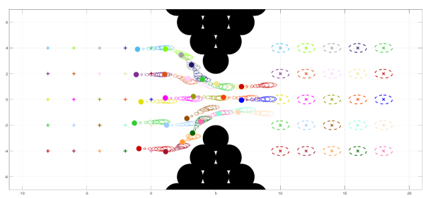
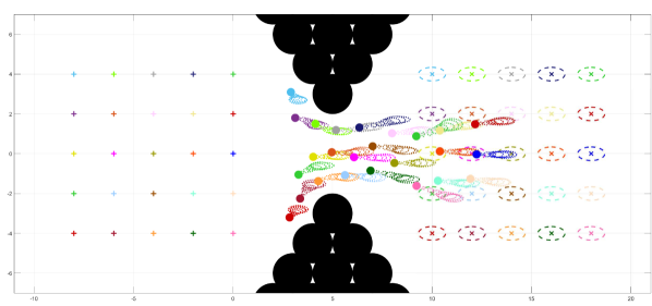
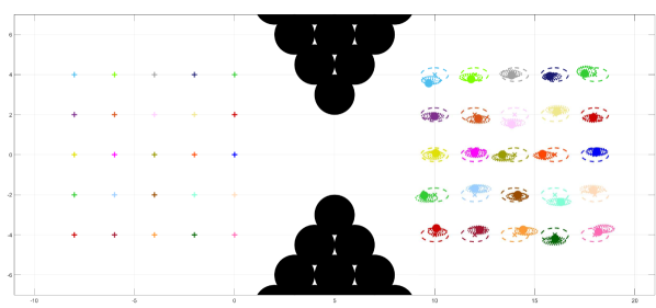
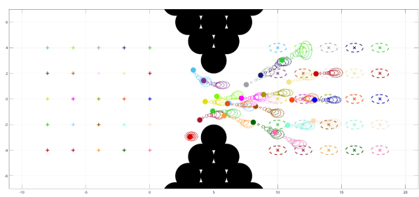
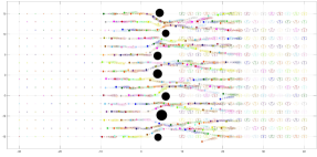
Figure 1: A task with $25$ robots required to pass through a narrow bottleneck before reaching their targets. Each snapshot shows their positions and planned distribution trajectories. Their initial positions are shown with “+”, while the $(\mu\pm 3\sigma)$ regions of the target distributions are shown as dashed ellipses with “x” at the center. The dotted ellipses illustrate the planned distribution trajectories at a particular timestep. Figures (a)-(c) show snapshots of DMPCS at $k=20,40,90$. Figure (d) shows a snapshot where a collison has occured when using a standard SMPC approach instead.

Figure 2: A large-scale multi-robot task where DMPCS steers 256 robots to their desired targets while ensuring their safety.

The execution of the proposed ADMM method of Section IV follows. First, the local decision variables $\bar{{\bm{u}}}_{i|k}^{\mathrm{aug}},{\bf L}_{i|k},{\bf K}_{i|k}$ of each robot are obtained (Line 12) through solving the local CS problems (22) as explained in Section IV-B. Afterwards, each robot $i$ receives the copy variables $\bar{{\bm{u}}}_{i|k}^{j}$ from all $j\in\pazocal{P}_{i|k}\backslash\{i\}$ (Line 13), so that it can compute ${\bm{g}}_{i|k}$ (Line 14) with (23). Subsequently, each robot $i$ receives the variables ${\bm{g}}_{j|k}$ from all $j\in\pazocal{V}_{i|k}\backslash\{i\}$ (Line 15), so that $\tilde{{\bm{g}}}_{i|k}$ is constructed and the dual updates (24) take place (Line 16). This iterative ADMM procedure is terminated after $\ell_{\mathrm{max}}$ iterations. Finally, the control input of each robot is computed (Line 19) through

$$u_{i,k|\kappa} =\bar{u}_{i,k|\kappa}+L_{i,k|\kappa}(\hat{x}_{i,\kappa}-\mu_{i,\kappa|\kappa})$$

$$~{}~{}~{}~{}~{}~{}~{}~{}~{}~{}~{}~{}~{}~{}~{}~{}~{}~{}~{}~{}~{}~{}~{}~{}~{}~{}+\sum^{k-1}_{l=0}K_{i,(k-1,l)|\kappa}\ w_{i,l}$$ (25)

where $\kappa$ is the last time $k$ that an MPC cycle took place. Note that in the special case where we assign $\hat{x}_{i,\kappa}=\mu_{i,\kappa|\kappa}$, the second term in the RHS of (25) becomes zero but this can change if the assumption of $\Sigma_{i,k|k}=0$ is relaxed.

Remark 3

All computations in DMPCS (Lines 7-9,12,14,16,19) can be performed in parallel by every robot $i\in\pazocal{V}$. In addition, all necessary communication steps (Lines 13,15) take place locally between neighboring robots. Therefore, the proposed algorithm is fully distributed in terms of computational and communication requirements.

Remark 4

The neighborhood adaptation that is performed in the beginning of every MPC cycle, based on the current positions of the robots, is an important advantage compared to the trajectory optimization approach followed in previous work [22], as it allows for using smaller adjustable neighborhoods and considering only collision avoidance constraints that are currently relevant. Except for enhancing safety, this also allows for using less copy variables, which further reduces dimensionality and computational demands.

VI Simulation Experiments

This sections presents simulation experiments that demonstrate the performance and scalability of DMPCS. In the main paper, we provide snapshots of the motion of the robots for two tasks, while we refer the reader to the supplementary video for the full experiments and additional tasks. In the following problem setup, all robots have unicycle dynamics with states $x_{i,k}=[\mathrm{x}_{i,k};\mathrm{y}_{i,k};\theta_{i,k};v_{i,k}]\in\mathbb{R}^{4}$ and inputs ${\bm{u}}_{i,k}=[a_{i,k};\omega_{i,k}]\in\mathbb{R}^{2}$, where $(\mathrm{x}_{i,k},\mathrm{y}_{i,k})$, $\theta_{i,k}$ $v_{i,k}$, $\omega_{i,k}$, $a_{i,k}$ are their 2D position coordinates, angles, linear and angular velocities and linear accelerations, respectively. In all experiments, we use $N_{\mathrm{pred}}=7$ and $N_{\mathrm{comp}}=2$. The discretization time step is $dt=0.05$. The process noise covariance is $W_{i}={\mathrm{diag}}(0.02,0.02,\pi/180,0.2)$. We set the control cost matrix $R_{i}={\mathrm{diag}}(10^{-2},10^{-2})$ and $\gamma_{i}=1$. For the collision avoidance constraints, we select $d_{i,o}=0.75$, $d_{i,j}=1.5$ and $\bar{\alpha}=\varphi^{-1}(0.997)=3$. Finally, we set $\rho=10^{-2},\ \ell_{\mathrm{max}}=30$ and $|\pazocal{V}_{i}|=6$.

In the first task, 25 robots are required to reach to their desired distribution targets while passing through a narrow “bottleneck” and avoiding collisions. The time horizon is set to $N_{\mathrm{total}}=90$. In Fig. 1(a)-1(c), the performance of DMPCS is demonstrated through three different snapshots that show the positions and planned distribution trajectories of the robots at the time. All robots successfully avoid collisions and reach to their desired distribution targets (Fig. 1(c)). For comparison purposes, in Fig. 1(d), we show a snapshot of the robots when using a standard SMPC approach that only optimizes for the feed-forward control inputs while using a fixed stabilizing feedback gain as in [9]. Unlike the CS approach, the standard SMPC cannot actively steer the covariances of the robots which leads to collisions as shown in the snapshot.

In the next task, we highlight the scalability of DMPCS to large-scale multi-robot problems. In particular, we consider a problem with 256 robots that need to move from one $16\times 16$ square grid to another one while avoiding collisions with each other and the obstacles in between. For this task, we used $N_{\mathrm{total}}=150$. Figure 2 shows a snapshot of the task at $k=40$, while the full task is available in the supplementary video. With DMPCS, all robots are successfully driven to their targets while maintaining their safety.

VII Conclusion

In this work, we propose DMPCS, a novel distributed SMPC algorithm for multi-robot control under uncertainty. Our approach combines CS theory using the Wasserstein distance and ADMM into an MPC scheme, to ensure safety while achieving scalability and parallelization. Numerical simulations verify the performance of DMPCS in various multi-robot navigation problems. The increased safety capability of the proposed method is also illustrated by comparing with standard SMPC approaches.

Appendix

VII-A Cost and Constraints Expressions

Following a similar derivation as in [32, Proposition 4], the cost $J_{i}^{\mathrm{dist}}$ can be written equivalently as

$$J_{i}^{\mathrm{dist}}(\bar{{\bm{u}}}_{i},{\bf L}_{i},{\bf K}_{i})=\sum_{k=1}^{K}\|{\bf T}_{i,k}{\bm{\eta}}_{i}(\bar{{\bm{u}}}_{i})-\mu_{i,\mathrm{f}}\|_{2}^{2}$$

$$+\|{\bm{\zeta}}_{i,k}({\bf L}_{i},{\bf K}_{i})\|_{F}^{2}+{\mathrm{tr}}(\Sigma_{i,\mathrm{f}})-2\|\sqrt{\Sigma_{i,\mathrm{f}}}{\bm{\zeta}}_{i,k}({\bf L}_{i},{\bf K}_{i})\|_{*},$$

where

$${\bm{\zeta}}_{i,k}({\bf L}_{i},{\bf K}_{i})={\bf T}_{i,k}\begin{bmatrix}{\bf G}_{i,0}+{\bf G}_{i,u}{\bf L}_{i}&{\bf G}_{i,w}+{\bf G}_{i,u}{\bf K}_{i}\end{bmatrix}.$$

The second part $J_{i}^{\mathrm{cont}}$ can be expressed as

$$J_{i}^{\mathrm{cont}}(\bar{{\bm{u}}}_{i},{\bf L}_{i},{\bf K}_{i}) =\bar{{\bm{u}}}_{i}^{\mathrm{T}}{\bf R}_{i}\bar{{\bm{u}}}_{i}+{\mathrm{tr}}({\bf R}_{i}{\bf L}_{i}\Sigma_{i,0}{\bf L}_{i}^{\mathrm{T}})$$

$$~{}~{}~{}~{}~{}+{\mathrm{tr}}({\bf R}_{i}{\bf K}_{i}{\bf W}_{i}{\bf K}_{i}^{\mathrm{T}})$$

where ${\bf R}_{i}={\mathrm{bdiag}}(R_{i},\dots,R_{i})\in\mathbb{R}^{Km_{i}\times Km_{i}}$. The proof for this expression consists of similar steps with the one in [32, Proposition 5] and is omitted due to space limitations.

The constraint (13) can be written as $a_{i}(\bar{{\bm{u}}}_{i},{\bf L}_{i},{\bf K}_{i})=[a_{i,0,};\dots;a_{i,K-1}]$ where each $a_{i,k}$ is given by

$$a_{i,k}(\bar{{\bm{u}}}_{i},{\bf L}_{i},{\bf K}_{i})=\bar{{\bm{u}}}_{i}^{\mathrm{T}}{\bf S}_{i,k}^{\mathrm{T}}R_{i}{\bf S}_{i,k}\bar{{\bm{u}}}_{i}+{\mathrm{tr}}({\bf S}_{i,k}^{\mathrm{T}}R_{i}{\bf S}_{i,k}{\bf L}_{i}\Sigma_{i,0}{\bf L}_{i}^{\mathrm{T}})$$

$$~{}~{}~{}~{}~{}~{}~{}~{}~{}~{}~{}~{}~{}~{}~{}~{}~{}~{}+{\mathrm{tr}}({\bf S}_{i,k}^{\mathrm{T}}R_{i}{\bf S}_{i,k}{\bf K}_{i}{\bf W}_{i}{\bf K}_{i}^{\mathrm{T}})-\gamma_{i}\leq 0.$$

The constraint (14) can be written as

$$b_{i}(\bar{{\bm{u}}}_{i}) =d_{i,o}+r_{o}-\|\mathbb{E}[p_{i,k}]-p_{o}\|_{2}$$

$$=d_{i,o}+r_{o}-\|H{\bf T}_{i,k}{\bm{\eta}}_{i}(\bar{{\bm{u}}}_{i})-p_{o}\|_{2}\leq 0.$$

Finally, the constraint (17) can be written as

$$c_{i,j}(\bar{{\bm{u}}}_{i},\bar{{\bm{u}}}_{j}) =d_{i,j}-\|\mathbb{E}[p_{i,k}]-\mathbb{E}[p_{j,k}]\|_{2}$$

$$=\|H{\bf T}_{i,k}{\bm{\eta}}_{i}(\bar{{\bm{u}}}_{i})-H{\bf T}_{j,k}{\bm{\eta}}_{j}(\bar{{\bm{u}}}_{j})\|_{2}\leq 0.$$

References

• [1] V. S. Chipade and D. Panagou, “Multiagent planning and control for swarm herding in 2-d obstacle environments under bounded inputs,” IEEE Transactions on Robotics, vol. 37, no. 6, pp. 1956–1972, 2021.
• [2] I. Maza, K. Kondak, M. Bernard, and A. Ollero, “Multi-uav cooperation and control for load transportation and deployment,” in Selected papers from the 2nd International Symposium on UAVs, Reno, Nevada, USA June 8–10, 2009.   Springer, 2009, pp. 417–449.
• [3] Y. Kantaros, M. Malencia, V. Kumar, and G. J. Pappas, “Reactive temporal logic planning for multiple robots in unknown environments,” in 2020 IEEE International Conference on Robotics and Automation (ICRA), 2020, pp. 11 479–11 485.
• [4] S. Heshmati-Alamdari, G. C. Karras, and K. J. Kyriakopoulos, “A predictive control approach for cooperative transportation by multiple underwater vehicle manipulator systems,” IEEE Transactions on Control Systems Technology, vol. 30, no. 3, pp. 917–930, 2022.
• [5] F. Rey, Z. Pan, A. Hauswirth, and J. Lygeros, “Fully decentralized ADMM for coordination and collision avoidance,” in 2018 European Control Conference (ECC), 2018, pp. 825–830.
• [6] L. Dai, Q. Cao, Y. Xia, and Y. Gao, “Distributed MPC for formation of multi-agent systems with collision avoidance and obstacle avoidance,” Journal of the Franklin Institute, vol. 354, no. 4, pp. 2068–2085, 2017.
• [7] X. Zhang, J. Ma, Z. Cheng, S. Huang, C. W. de Silva, and T. H. Lee, “Improved hierarchical ADMM for nonconvex cooperative distributed model predictive control,” arXiv preprint arXiv:2011.00463, 2020.
• [8] S. Yan, P. J. Goulart, and M. Cannon, “Stochastic MPC with dynamic feedback gain selection and discounted probabilistic constraints,” IEEE Transactions on Automatic Control, 2021.
• [9] E. Arcari, A. Iannelli, A. Carron, and M. N. Zeilinger, “Stochastic MPC with robustness to bounded parametric uncertainty,” arXiv preprint arXiv:2205.10275, 2022.
• [10] G. Schildbach, L. Fagiano, C. Frei, and M. Morari, “The scenario approach for stochastic model predictive control with bounds on closed-loop constraint violations,” Automatica, vol. 50, no. 12, pp. 3009–3018, 2014.
• [11] F. Oldewurtel, C. N. Jones, and M. Morari, “A tractable approximation of chance constrained stochastic MPC based on affine disturbance feedback,” in 2008 47th IEEE conference on decision and control.   IEEE, 2008, pp. 4731–4736.
• [12] K. Okamoto and P. Tsiotras, “Stochastic model predictive control for constrained linear systems using optimal covariance steering,” arXiv preprint arXiv:1905.13296, 2019.
• [13] I. M. Balci, E. Bakolas, B. Vlahov, and E. A. Theodorou, “Constrained covariance steering based tube-MPPI,” in 2022 American Control Conference (ACC).   IEEE, 2022, pp. 4197–4202.
• [14] J. Yin, Z. Zhang, E. Theodorou, and P. Tsiotras, “Trajectory distribution control for model predictive path integral control using covariance steering,” in 2022 International Conference on Robotics and Automation (ICRA).   IEEE, 2022, pp. 1478–1484.
• [15] A. Hotz and R. E. Skelton, “Covariance control theory,” Int. J. Control., vol. 46, no. 1, pp. 13–32, 1987.
• [16] J.-H. Xu and R. E. Skelton, “An improved covariance assignment theory for discrete systems,” IEEE Trans. Automat. Contr., vol. 37, no. 10, pp. 1588–1591, 1992.
• [17] Y. Chen, T. T. Georgiou, and M. Pavon, “Optimal steering of a linear stochastic system to a final probability distribution, part i,” IEEE Trans. Automat. Contr., vol. 61, no. 5, pp. 1158–1169, 2015.
• [18] G. Kotsalis, G. Lan, and A. S. Nemirovski, “Convex optimization for finite-horizon robust covariance control of linear stochastic systems,” SIAM Journal on Control and Optimization, vol. 59, no. 1, pp. 296–319, 2021.
• [19] I. M. Balci and E. Bakolas, “Exact SDP formulation for discrete-time covariance steering with Wasserstein terminal cost,” arXiv preprint arXiv:2205.10740, 2022.
• [20] F. Liu, G. Rapakoulias, and P. Tsiotras, “Optimal covariance steering for discrete-time linear stochastic systems,” arXiv preprint arXiv:2211.00618, 2022.
• [21] K. Okamoto and P. Tsiotras, “Optimal stochastic vehicle path planning using covariance steering,” IEEE Robot. Autom. Lett., vol. 4, no. 3, pp. 2276–2281, 2019.
• [22] A. D. Saravanos, A. Tsolovikos, E. Bakolas, and E. Theodorou, “Distributed Covariance Steering with Consensus ADMM for Stochastic Multi-Agent Systems,” in Proceedings of Robotics: Science and Systems, Virtual, July 2021.
• [23] C. R. Givens and R. M. Shortt, “A class of Wasserstein metrics for probability distributions.” Michigan Mathematical Journal, vol. 31, no. 2, pp. 231–240, 1984.
• [24] T. Halsted, O. Shorinwa, J. Yu, and M. Schwager, “A survey of distributed optimization methods for multi-robot systems,” arXiv preprint arXiv:2103.12840, 2021.
• [25] Z. Cheng, J. Ma, X. Zhang, C. W. de Silva, and T. H. Lee, “ADMM-based parallel optimization for multi-agent collision-free model predictive control,” arXiv preprint arXiv:2101.09894, 2021.
• [26] A. D. Saravanos, Y. Aoyama, H. Zhu, and E. A. Theodorou, “Distributed differential dynamic programming architectures for large-scale multi-agent control,” arXiv preprint arXiv:2207.13255, 2022.
• [27] M. A. Pereira, A. D. Saravanos, O. So, and E. A. Theodorou, “Decentralized Safe Multi-agent Stochastic Optimal Control using Deep FBSDEs and ADMM,” in Proceedings of Robotics: Science and Systems, New York City, NY, USA, June 2022.
• [28] J. Ridderhof, K. Okamoto, and P. Tsiotras, “Nonlinear uncertainty control with iterative covariance steering,” in 2019 IEEE 58th Conference on Decision and Control (CDC).   IEEE, 2019, pp. 3484–3490.
• [29] E. Bakolas and A. Tsolovikos, “Greedy finite-horizon covariance steering for discrete-time stochastic nonlinear systems based on the unscented transform,” in 2020 American Control Conference (ACC).   IEEE, 2020, pp. 3595–3600.
• [30] Z. Yi, Z. Cao, E. Theodorou, and Y. Chen, “Nonlinear covariance control via differential dynamic programming,” in 2020 American Control Conference (ACC).   IEEE, 2020, pp. 3571–3576.
• [31] I. M. Balci and E. Bakolas, “Covariance steering of discrete-time stochastic linear systems based on wasserstein distance terminal cost,” IEEE Control Systems Letters, vol. 5, no. 6, pp. 2000–2005, 2021.
• [32] ——, “Covariance control of discrete-time gaussian linear systems using affine disturbance feedback control policies,” in 2021 60th IEEE Conference on Decision and Control (CDC), 2021, pp. 2324–2329.
• [33] A. L. Yuille and A. Rangarajan, “The concave-convex procedure,” Neural computation, vol. 15, no. 4, pp. 915–936, 2003.
• [34] F. Augugliaro, A. P. Schoellig, and R. D’Andrea, “Generation of collision-free trajectories for a quadrocopter fleet: A sequential convex programming approach,” in 2012 IEEE/RSJ International Conference on Intelligent Robots and Systems, 2012, pp. 1917–1922.