From CNNs to Shift-Invariant Twin Models Based on Complex Wavelets

Abstract

We propose a novel antialiasing method to increase shift invariance and prediction accuracy in convolutional neural networks. Specifically, we replace the first-layer combination “real-valued convolutions $\to$ max pooling” ($\mathbb{R}$Max) by “complex-valued convolutions $\to$ modulus” ($\mathbb{C}$Mod), which is stable to translations. To justify our approach, we claim that $\mathbb{C}$Mod and $\mathbb{R}$Max produce comparable outputs when the convolution kernel is band-pass and oriented (Gabor-like filter). In this context, $\mathbb{C}$Mod can be considered as a stable alternative to $\mathbb{R}$Max. Thus, prior to antialiasing, we force the convolution kernels to adopt such a Gabor-like structure. The corresponding architecture is called mathematical twin, because it employs a well-defined mathematical operator to mimic the behavior of the original, freely-trained model. Our antialiasing approach achieves superior accuracy on ImageNet and CIFAR-10 classification tasks, compared to prior methods based on low-pass filtering. Arguably, our approach’s emphasis on retaining high-frequency details contributes to a better balance between shift invariance and information preservation, resulting in improved performance. Furthermore, it has a lower computational cost and memory footprint than concurrent work, making it a promising solution for practical implementation.

1 Introduction

Over the past decade, some progress has been made on understanding the strengths and limitations of convolutional neural networks (CNNs) for computer vision [21, 35, 41]. The ability of CNNs to embed input images into a feature space with linearly separable decision regions is a key factor to achieve high classification accuracy. An important property to reach this linear separability is the ability to discard or minimize non-discriminative image components. In particular, feature vectors are expected to be stable with respect to translations [35]. However, subsampling operations, typically found in convolution and pooling layers, are an important source of instability—a phenomenon known as aliasing [1]. A few approaches have attempted to address this issue.

Blurpooled CNNs.

Zhang [42] proposed to apply a low-pass blurring filter before each subsampling operation in CNNs. Specifically, 1. max pooling layers ($\mbox{Max}\to\mbox{Sub}$) are replaced by max-blur pooling ($\mbox{Max}\to\mbox{Blur}\to\mbox{Sub}$); 2. convolution layers followed by ReLU ($\mbox{Conv}\to\mbox{Sub}\to\mbox{ReLU}$) are blurred before subsampling ($\mbox{Conv}\to\mbox{ReLU}\to\mbox{Blur}\to\mbox{Sub}$). The combination $\mbox{Blur}\to\mbox{Sub}$ is referred to as blur pooling. This approach follows a well-known practice in signal processing, which involves low-pass filtering a high-frequency signal before subsampling, in order to avoid artifacts in reconstruction. Their approach improved the shift invariance as well as the accuracy of CNNs trained on ImageNet and CIFAR-10 datasets. However, this was achieved with a significant loss of information.

A question then arises: is it possible to design a non-destructive antialiasing method, and if so, does it further improve accuracy? In a more recent work, Zou et al. [45] tackled this question through an adaptive antialiasing approach, called adaptive blur pooling. In this nonlinear setting, the blurring filter varies across channels and image locations, therefore preserving high-frequency information in strategic zones. Albeit achieving higher prediction accuracy, this approach remains fundamentally based on low-pass filtering. Consequently, features that are not blurred may still be unstable to translations. Furthermore, adaptive blur pooling requires additional memory, computational resources, and trainable parameters.

Proposed Approach.

In this paper, we propose an alternative antialiasing approach based on complex-valued convolutions, extracting high-frequency features that are stable to translations. We observed improved accuracy for ImageNet and CIFAR-10 classification, compared to the two antialiasing methods based on blur pooling [42, 45]. Furthermore, our approach offers significant advantages in terms of computational efficiency and memory usage, and does not induce any additional training, unlike adaptive blur pooling.

Our proposed method replaces the first layers of a CNN:

$$\mbox{Conv}\to\mbox{Sub}\to\mbox{Bias}\to\mbox{ReLU}\to\mbox{MaxPool},$$ (1)

equivalently written as

$$\mbox{Conv}\to\mbox{Sub}\to\mbox{MaxPool}\to\mbox{Bias}\to\mbox{ReLU},$$ (2)

by the following combination:

$$\mathbb{C}\mbox{Conv}\to\mbox{Sub}\to\mbox{Modulus}\to\mbox{Bias}\to\mbox{ReLU},$$ (3)

where $\mathbb{C}$Conv denotes a convolution operator with a complex-valued kernel, whose real and imaginary parts approximately form a 2D Hilbert transform pair [11]. From (2) and (3), we introduce the two following operators:

$$\mathbb{R}\mbox{Max}\; :\;\mbox{Conv}\to\mbox{Sub}\to\mbox{MaxPool};$$ (4)

$$\mathbb{C}\mbox{Mod}\; :\;\mathbb{C}\mbox{Conv}\to\mbox{Sub}\to\mbox{Modulus}.$$ (5)

Our method is motivated by the following theoretical claim. In a recent paper submission [23], we proved that 1. $\mathbb{C}$Mod is nearly invariant to translations, if the convolution kernel is band-pass and clearly oriented; 2. $\mathbb{R}$Max and $\mathbb{C}$Mod produce comparable outputs, except for some filter frequencies regularly scattered across the Fourier domain. We then combined these two properties to establish a stability metric for $\mathbb{R}$Max as a function of the convolution kernel’s frequency vector. This work was essentially theoretical, with limited experiments conducted on a deterministic model solely based on the dual-tree complex wavelet packet transform (DT-$\mathbb{C}$WPT). However, it lacked applications to tasks such as image classification. Building upon this theoretical study, in this paper, we consider the $\mathbb{C}$Mod operator as a proxy for $\mathbb{R}$Max, extracting comparable, yet more stable features.

In compliance with the theory, the $\mathbb{R}$Max-$\mathbb{C}$Mod substitution is only applied to the output channels associated with oriented band-pass filters, referred to as Gabor-like kernels. This kind of structure is known to arise spontaneously in the first layer of CNNs trained on image datasets such as ImageNet [38]. In this paper, we enforce this property by applying additional constraints to the original model, prior to antialiasing. Specifically, a predefined number of convolution kernels are guided to adopt Gabor-like structures, instead of letting the network learn them from scratch. For this purpose, we rely on the dual-tree complex wavelet packet transform (DT-$\mathbb{C}$WPT) [2]. Throughout the paper, we refer to this constrained model as a mathematical twin, because it employs a well-defined mathematical operator to mimic the behavior of the original model. In this context, replacing $\mathbb{R}$Max by $\mathbb{C}$Mod is straightforward, since the complex-valued filters are provided by DT-$\mathbb{C}$WPT.

Other Related Work.

Following the ideas developed for antialiasing, Chaman and Dokmanic [5] reached perfect shift invariance by using an adaptive, input-dependent subsampling grid, whereas previous models rely on fixed grids. This idea was harnessed by Xu et al. [37] to get shift equivariance in generative models. This approach is not intended to compete with other antialiasing methods, but rather to complement them at the subsampling stages.

Another aspect of shift invariance in CNNs is related to boundary effects. The fact that CNNs can encode the absolute position of an object in the image by exploiting boundary effects was discovered independently by Islam et al. [15], and Kayhan and Gemert [17]. This phenomenon is left outside the scope of our paper.

Wavelet scattering networks (ScatterNets), by Bruna and Mallat [4], perform cascading wavelet convolutions and nonlinear operations. They produce shift-invariant image representations that are stable to deformation and preserve high-frequency information. Further extensions include roto-translation invariant ScatterNets [27], hybrid ScatterNets combined with fully-trained layers [26] or dictionary learning [40], dual-tree complex wavelet ScatterNets [31], graph ScatterNets [44], learnable ScatterNets via feature map mixing [6] or parametric wavelet filters [9]. As deep learning architectures with well-defined mathematical properties, ScatterNets may be used as explanatory models for standard, freely-trained networks. However, there is no exact correspondence between the two types of architectures [34]. In contrast, our models are enhanced versions of existing networks, rather than ad hoc constructions. This allows to draw comparisons in terms of prediction accuracy and shift invariance.

Finally, we draw the reader’s attention to the family of complex-valued CNNs ($\mathbb{C}$VCNNs), which is the focus of a comprehensive survey [22]. These networks are well suited for tasks requiring the phase information to be propagated through the entire network, as done in the context of magnetic resonance imaging [7], polarimetric imaging [43] or audio signals [33]. However, for image recognition tasks, $\mathbb{C}$VCNNs do not seem to perform better than standard CNNs, with equal number of trainable parameters [33]. Conversely, our approach discards the phase information by computing the modulus. In summary, $\mathbb{C}$VCNNs and our models, although both employing complex-valued convolutions, are suited for different contexts.

2 Proposed Approach

We first describe the general principles of our antialiasing approach based on complex convolutions. We then provide some details about the mathematical twin based on DT-$\mathbb{C}$WPT, and explain how our method has been benchmarked against blur-pooling-based antialiased models.

We represent feature maps as 2D sequences, defined by straight capital letters: $\mathrm{X}\in\mathcal{S}$. Indexing is denoted by square brackets: for any 2D index $\boldsymbol{n}\in\mathbb{Z}^{2}$, $\mathrm{X}[\boldsymbol{n}]\in\mathbb{R}$ or $\mathbb{C}$. The cross-correlation between $\mathrm{X}$ and $\mathrm{V}\in\mathcal{S}$ is defined by $(\mathrm{X}\star\mathrm{V})[\boldsymbol{n}]:=\sum_{\boldsymbol{k}\in\mathbb{Z}^{2}}\mathrm{X}[\boldsymbol{n}+\boldsymbol{k}]\,\mathrm{V}[\boldsymbol{k}]$. The down arrow refers to subsampling: for any $m\in\mathbb{N}^{*}$, $(\mathrm{X}\downarrow m)[\boldsymbol{n}]:=\mathrm{X}[m\boldsymbol{n}]$.

2.1 Standard Architectures

A convolution layer with $K$ input channels, $L$ output channels and subsampling factor $m\in\mathbb{N}\setminus\{0\}$ is parameterized by a weight tensor $\mathbf{V}:=(\mathrm{V}_{lk})_{l\in\left\{1\mathinner{\ldotp\ldotp}L\right\},\,k\in\left\{1\mathinner{\ldotp\ldotp}K\right\}}\in\mathcal{S}^{L\times K}$. For any multichannel input $\mathbf{X}:=(\mathrm{X}_{k})_{k\in\left\{1\mathinner{\ldotp\ldotp}K\right\}}\in\mathcal{S}^{K}$, the corresponding output $\mathbf{Y}:=(\mathrm{Y}_{l})_{l\in\left\{1\mathinner{\ldotp\ldotp}L\right\}}\in\mathcal{S}^{L}$ is defined such that, for any output channel $l\in\left\{1\mathinner{\ldotp\ldotp}L\right\}$,

$$\mathrm{Y}_{l}:=\sum_{k=1}^{K}(\mathrm{X}_{k}\star\mathrm{V}_{lk})\downarrow m.$$ (6)

For instance, in AlexNet and ResNet, $K=3$ (RGB input images), $L=64$, and $m=4$ and $2$, respectively. Next, a bias $\boldsymbol{b}:=(b_{1},\,\cdots,\,b_{L})^{\top}\in\mathbb{R}^{L}$ is applied to $\mathbf{Y}$, which is then transformed through nonlinear ReLU and max pooling operators. The activated outputs satisfy

$$\mathrm{A}^{\operatorname{max}}_{l}:=\operatorname{MaxPool}\left(\operatorname{ReLU}(\mathrm{Y}_{l}+b_{l})\right),$$ (7)

where we have defined, for any $\mathrm{Y}\in\mathcal{S}$ and any $\boldsymbol{n}\in\mathbb{Z}^{2}$,

$$\operatorname{ReLU}(\mathrm{Y})[\boldsymbol{n}] :=\max(0,\,\mathrm{Y}[\boldsymbol{n}]);$$ (8)

$$\operatorname{MaxPool}(\mathrm{Y})[\boldsymbol{n}] :=\max_{\left\|\boldsymbol{k}\right\|_{\infty}\leq 1}\mathrm{Y}[2\boldsymbol{n}+\boldsymbol{k}].$$ (9)

2.2 Antialiasing Principle

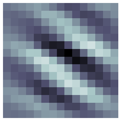
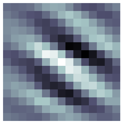
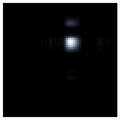
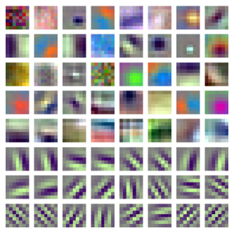
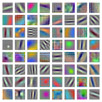
We consider the first convolution layer of a CNN, as described in (6). As widely discussed in the literature [38], after training with ImageNet, a certain number of convolution kernels $\mathrm{V}_{lk}$ spontaneously take the appearance of oriented waveforms with well-defined frequency and orientation (Gabor-like kernels), as illustrated in Fig. 1(a). A visual representation of trained convolution kernels is provided in Appendix E. In this paper, we refer to the corresponding output channels $l\in\mathcal{G}\subset\left\{1\mathinner{\ldotp\ldotp}L\right\}$ as Gabor channels. The main idea is to substitute, for any $l\in\mathcal{G}$, $\mathbb{R}$Max by $\mathbb{C}$Mod, as explained hereafter. Following (2), expression (7) can be rewritten

$$\mathrm{A}^{\operatorname{max}}_{l}=\operatorname{ReLU}\bigl{(}\mathrm{Y}^{\operatorname{max}}_{l}+b_{l}\bigr{)},$$ (10)

where $\mathrm{Y}^{\operatorname{max}}_{l}$ is the output of an $\mathbb{R}$Max operator as introduced in (4). More formally,

$$\mathrm{Y}^{\operatorname{max}}_{l}:=\operatorname{MaxPool}\left(\sum_{k=1}^{K}(\mathrm{X}_{k}\star\mathrm{V}_{lk})\downarrow m\right).$$ (11)

Then, following (3), the $\mathbb{R}$Max-$\mathbb{C}$Mod substitution yields

$$\mathrm{A}^{\operatorname{mod}}_{l}=\operatorname{ReLU}\bigl{(}\mathrm{Y}^{\operatorname{mod}}_{l}+b_{l}\bigr{)},$$ (12)

where $\mathrm{Y}^{\operatorname{mod}}_{l}$ is the output of a $\mathbb{C}$Mod operator (5), satisfying

$$\mathrm{Y}^{\operatorname{mod}}_{l}:=\left|\sum_{k=1}^{K}(\mathrm{X}_{k}\star\mathrm{W}_{lk})\downarrow(2m)\right|.$$ (13)

In the above expression, $\mathrm{W}_{lk}$ is a complex-valued analytic kernel satisfying

$$\mathrm{W}_{lk}:=\mathrm{V}_{lk}+i\mathcal{H}(\mathrm{V}_{lk}),$$ (14)

where $\mathcal{H}$ denotes the two-dimensional Hilbert transform as introduced by Havlicek et al. [11]. It is defined, for any real-valued filter $\mathrm{V}\in\mathcal{S}$ and any frequency vector $\boldsymbol{\xi}:=(\xi_{1},\,\xi_{2})^{\top}\in\left[-\pi,\,\pi\right]^{2}$, by

$$\widehat{\mathcal{H}\mathrm{V}}(\boldsymbol{\xi}):=-i\operatorname{sgn}(\xi_{1})\,\widehat{\mathrm{V}}(\boldsymbol{\xi}).$$ (15)

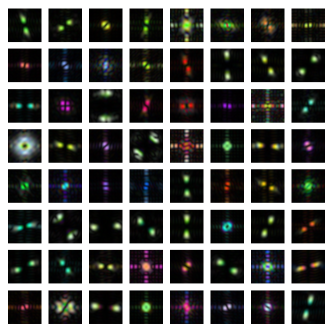
The Hilbert transform is designed such that the Fourier transform of $\mathrm{W}_{lk}$ is entirely supported in the half-plane of nonnegative $x$-values. Therefore, since $\mathrm{V}_{lk}$ is Gabor-like, the energy of $\mathrm{W}_{lk}$ is concentrated within a small window in the Fourier domain, as depicted in Fig. 1(d). Due to this property, the modulus operator provides a smooth envelope for complex-valued cross-correlations with $\mathrm{W}_{lk}$ [19]. This leads to the output $\mathrm{Y}^{\operatorname{mod}}_{l}$ (13) being nearly invariant to translations. Additionally, the subsampling factor in (13) is twice that in (11), to account for the factor-$2$ subsampling achieved through max pooling (9).

(a)

(b)

(c)

(d)

Figure 1: (a), (b): Real and imaginary parts of a Gabor-like convolution kernel $\mathrm{W}_{lk}:=\mathrm{V}_{lk}+i\mathcal{H}(\mathrm{V}_{lk})$, forming a 2D Hilbert transform pair. (c), (d): Power spectra (energy of the Fourier transform) of $\mathrm{V}_{lk}$ and $\mathrm{W}_{lk}$, respectively.

2.3 Wavelet-Based Twin Models (WCNNs)

As explained in Sec. 2.2, introducing an imaginary part to the Gabor-like convolution kernels improves shift invariance. Our antialiasing method therefore restricts to the Gabor channels $l\in\mathcal{G}\subset\left\{1\mathinner{\ldotp\ldotp}L\right\}$. However, $\mathcal{G}$ is unknown a priori: for a given output channel $l\in\left\{1\mathinner{\ldotp\ldotp}L\right\}$, whether $\mathrm{V}_{lk}$ will become band-pass and oriented after training is unpredictable. Thus, we need a way to automatically separate the set $\mathcal{G}$ of Gabor channels from the set of remaining channels, denoted by $\mathcal{F}:=\left\{1\mathinner{\ldotp\ldotp}L\right\}\setminus\mathcal{G}$. To this end, we built “mathematical twins” of standard CNNs, based on the dual-tree wavelet packet transform (DT-$\mathbb{C}$WPT). These models, which we call WCNNs in short, reproduce the behavior of freely-trained architectures with a higher degree of control and fewer trainable parameters. In this section, we present their general structure; a more detailed description is provided in Appendix A. For the purpose of readability, we assume that $K=3$ (RGB input images).

We denote by $L_{\operatorname{gabor}}:=\operatorname{card}(\mathcal{G})$ and $L_{\operatorname{free}}:=\operatorname{card}(\mathcal{F})$ the number of Gabor and remaining channels, respectively. They are determined empirically from the trained CNNs—see Tab. 1. In a twin WCNN architecture, the two groups of output channels are organized such that $\mathcal{F}=\left\{1\mathinner{\ldotp\ldotp}L_{\operatorname{free}}\right\}$ and $\mathcal{G}=\left\{(L_{\operatorname{free}}+1)\mathinner{\ldotp\ldotp}L\right\}$. The first $L_{\operatorname{free}}$ channels, which are outside the scope of our antialiasing approach, remain freely-trained as in the standard architecture. Regarding the $L_{\operatorname{gabor}}$ Gabor channels, the convolution kernels $\mathrm{V}_{lk}$ are constrained to satisfy the following requirements. First, all three RGB input channels are processed with the same filter, up to a multiplicative constant. More formally, there exists a luminance weight vector $\boldsymbol{\mu}:=(\mu_{1},\,\mu_{2},\,\mu_{3})^{\top}$, with $\mu_{k}\in\left[0,\,1\right]$ and $\sum_{k=1}^{3}\mu_{k}=1$, such that,

$$\forall k\in\left\{1\mathinner{\ldotp\ldotp}3\right\},\,\mathrm{V}_{lk}=\mu_{k}\widetilde{\mathrm{V}}_{l},$$ (16)

where $\widetilde{\mathrm{V}}_{l}:=\sum_{k=1}^{3}\mathrm{V}_{lk}$ denotes the mean kernel. Furthermore, $\widetilde{\mathrm{V}}_{l}$ must be band-pass and oriented (Gabor-like filter). The following paragraphs explain how these two constraints are implemented in our WCNN architecture.

Monochrome Filters.

Expression (16) is actually a property of standard CNNs: the oriented band-pass RGB kernels generally appear monochrome (see kernel visualization of freely-trained CNNs Appendix E). A numerical assessment of this property can by found in [23]. In WCNNs, this constraint is implemented with a trainable $1\times 1$ convolution layer [24], parameterized by $\boldsymbol{\mu}$, computing the following luminance image:

$$\mathrm{X}^{\operatorname{lum}}:=\sum_{k=1}^{3}\mu_{k}\mathrm{X}_{k}.$$ (17)

(a) WAlexNet ($32$ Gabor channels)

(b) WResNet ($24$ Gabor channels)

Figure 2: Convolution kernels in the first layer of WAlexNet (a) and WResNet-34 (b), after training with ImageNet-1K. For each output channel $l\in\left\{1\mathinner{\ldotp\ldotp}64\right\}$, the corresponding convolution kernel $(\mathrm{V}_{lk})_{k\in\left\{1\mathinner{\ldotp\ldotp}3\right\}}$ is displayed as an RGB image in the spatial domain (left), and its associated magnitude spectrum in the Fourier domain (right). The convolution kernels associated to the Gabor channels are displayed on the $4$ and $3$ last rows for WAlexNet and WResNet, respectively. For the sake of visual rendering, they have been respectively cropped to $(11\times 11)$ and $(7\times 7)$ to match the size of the freely-trained kernels.

(a) AlexNet

(b) WAlexNet (baseline)

(c) $\mathbb{C}$WAlexNet (proposed approach)

Figure 3: First layers of AlexNet and its variants, corresponding to a convolution layer followed by ReLU and max pooling (1). The models are framed according to the same colors and line styles as in Figs. 4 and 5. The green modules are the ones containing trainable parameters; the orange and purple modules represent static linear and nonlinear operators, respectively. The numbers between each module represent the depth (number of channels), height and width of each output. Fig. 3(a): freely-trained models. Top: standard AlexNet. Bottom: Zhang’s “blurpooled” AlexNet. Fig. 3(b): mathematical twins (WAlexNet) reproducing the behavior of standard (top) and blurpooled (bottom) AlexNet. The left side of each diagram corresponds to the $L_{\operatorname{free}}:=32$ freely-trained output channels, whereas the right side displays the $L_{\operatorname{gabor}}:=32$ remaining channels, where freely-trained convolutions have been replaced by a wavelet block (WBlock) as described in Sec. 2.3. Fig. 3(c): $\mathbb{C}$Mod-based antialiased WAlexNet, where WBlock has been replaced by $\mathbb{C}$WBlock, and max pooling by a modulus. The bias and ReLU are placed after the modulus, following (3). In the bottom models, we compare Zhang’s antialiasing approach (Fig. 3(b)) with ours (Fig. 3(c)) in the Gabor channels.

 

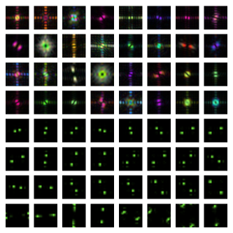
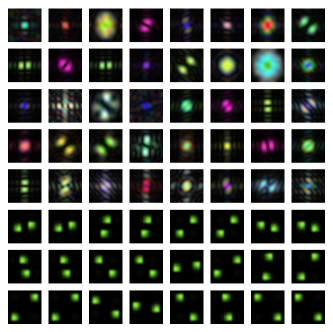
Gabor-Like Kernels. To guarantee the Gabor-like property on $\widetilde{\mathrm{V}}_{l}$, we implemented DT-$\mathbb{C}$WPT, which is achieved through a series of subsampled convolutions. The number of decomposition stages $0pt\in\mathbb{N}\setminus\{0\}$ was chosen such that $m=2^{0pt-1}$, where, as a reminder, $m$ denotes the subsampling factor as introduced in (6). DT-$\mathbb{C}$WPT generates a set of filters $\bigl{(}\mathrm{W}^{\operatorname{dt}}_{k^{\prime}}\bigr{)}_{k^{\prime}\in\left\{1\mathinner{\ldotp\ldotp}4\times 4^{0}pt\right\}}$, which tiles the Fourier domain $\left[-\pi,\,\pi\right]^{2}$ into $4\times 4^{0}pt$ overlapping square windows. Their real and imaginary parts approximately form a 2D Hilbert transform pair such as defined in (15).

The WCNN architecture is designed such that, for any Gabor channel $l\in\mathcal{G}$, $\widetilde{\mathrm{V}}_{l}$ is the real part of one such filter:

$$\exists k^{\prime}\in\left\{1\mathinner{\ldotp\ldotp}4\times 4^{0}pt\right\}:\widetilde{\mathrm{V}}_{l}=\operatorname{Re}\bigl{(}\mathrm{W}^{\operatorname{dt}}_{k^{\prime}}\bigr{)}.$$ (18)

The output $\mathrm{Y}_{l}$ introduced in (6) then becomes

$$\mathrm{Y}_{l}=\bigl{(}\mathrm{X}^{\operatorname{lum}}\star\widetilde{\mathrm{V}}_{l}\bigr{)}\downarrow 2^{0pt-1}.$$ (19)

To summarize, a WCNN substitutes the freely-trained convolution (6) with a combination of (17) and (19), for any Gabor output channels $l\in\mathcal{G}$. This combination is wrapped into a wavelet block, also referred to as WBlock in short. Technical details about its exact design are provided Appendix A. Note that the Fourier resolution of $\mathrm{V}_{lk}$ increases with the subsampling factor $m$. This property is consistent with what is observed in freely-trained CNNs: in AlexNet, where $m=4$, the Gabor-like filters are more localized in frequency (and less spatially localized) than in ResNet, where $m=2$.

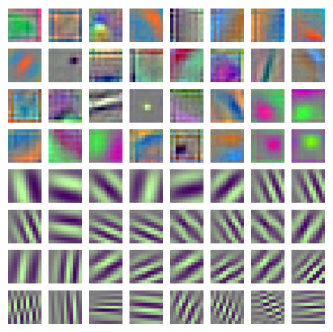
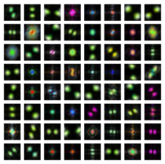
Figure 2 displays the kernels $\mathbf{V}\in\mathcal{S}^{L\times K}$, with $K=3$ and $L=64$, for the WCNN architectures based on AlexNet and ResNet, which we refer to as WAlexNet and WResNet, respectively. In these models, $m=4$ and $2$, which implies $0pt=3$ and $2$, respectively. The kernels are shown as RGB color images, after training with ImageNet, for both freely-trained and Gabor channels.

Antialiased WCNNs.

Using the antialiasing principles presented in Sec. 2.2, we replace $\mathbb{R}$Max (11) by $\mathbb{C}$Mod (13) for all Gabor channels $l\in\mathcal{G}$. In the corresponding model, referred to as $\mathbb{C}$WCNN, the wavelet block is replaced by a complex wavelet block ($\mathbb{C}$WBlock), in which (19) becomes

$$\mathrm{Z}_{l}=\bigl{(}\mathrm{X}^{\operatorname{lum}}\star\widetilde{\mathrm{W}}_{l}\bigr{)}\downarrow 2^{0pt},$$ (20)

where $\widetilde{\mathrm{W}}_{l}$ is obtained by considering both real and imaginary parts of the DT-$\mathbb{C}$WPT filter (18). Then, a modulus is applied to $\mathrm{Z}_{l}$, which yields $\mathrm{Y}^{\operatorname{mod}}_{l}$ such as defined in (13), with $\mathrm{W}_{lk}:=\mu_{k}\widetilde{\mathrm{W}}_{l}$ for any RGB channel $k\in\left\{1\mathinner{\ldotp\ldotp}3\right\}$. Finally, we apply a bias and ReLU to $\mathrm{Y}^{\operatorname{mod}}_{l}$, following (12).

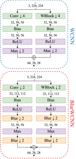
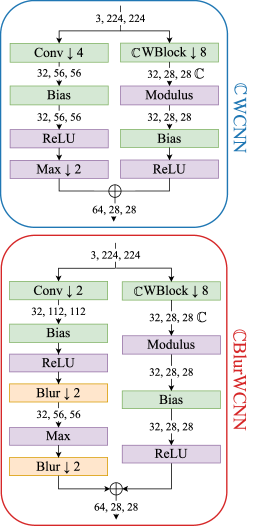
A schematic representation of WAlexNet and its antialiased version, referred to as $\mathbb{C}$WAlexNet, is provided in Figs. 3(b) and 3(c) (top).

2.4 WCNNs with Blur Pooling

We benchmark our approach against the antialiasing methods proposed by Zhang [42] and Zou et al. [45]. To this end, we first consider a WCNN antialiased with static or adaptive blur pooling, respectively referred to as BlurWCNN and ABlurWCNN. A schematic representation of BlurWAlexNet is provided in Fig. 3(b) (bottom). Then, we substitute the blurpooled Gabor channels (right branch of the diagram) with our own $\mathbb{C}$Mod-based approach. The corresponding models are respectively referred to as $\mathbb{C}$BlurWCNN and $\mathbb{C}$ABlurWCNN. Again, a schematic representation of $\mathbb{C}$BlurWAlexNet can be found in Fig. 3(c) (bottom). Note that, for a fair comparison, all models use blur pooling in the freely-trained channels as well as deeper layers. Therefore, several antialiasing methods are employed in different parts of the network.

2.5 Adaptation to ResNet: Batch Normalization

In many architectures including ResNet, the bias is computed after an operation called batch normalization (BN) [14]. In this context, (1) becomes

$$\mbox{Conv}\to\mbox{Sub}\to\mbox{BN}\to\mbox{Bias}\to\mbox{ReLU}\to\mbox{MaxPool}.$$ (21)

As detailed in Appendix B, the $\mathbb{R}$Max-$\mathbb{C}$Mod substitution yields, analogously to (3),

$$\mathbb{C}\mbox{Conv}\!\to\!\mbox{Sub}\!\to\!\mbox{Modulus}\!\to\!\mbox{BN}0\!\to\!\mbox{Bias}\!\to\!\mbox{ReLU},$$ (22)

where BN$0$ refers to a special type of batch normalization without mean centering. A schematic representation of ResNet-based models, as done in Fig. 3(a) for AlexNet, is provided in Fig. 8(a).

3 Experiments

	WAlexNet	WResNet
$m$ (subsampling factor)	$4$	$2$
$0pt$ (decomposition depth)	$3$	$2$
$L_{\operatorname{free}},\,L_{\operatorname{gabor}}$ (output channels)	$32,\,32$	$40,\,24$

Table 1: Experimental settings for our WCNN twin models. Other details are provided in Appendix C.

3.1 Experiment Details

ImageNet. We built our WCNN and $\mathbb{C}$WCNN twin models based on AlexNet [20] and ResNet-34 [12]. Their overall design is described in Sec. 2, along with setting details in Tab. 1. The values of $L_{\operatorname{free}}$ and $L_{\operatorname{gabor}}$ were determined empirically from the freely-trained AlexNet and ResNet-34; further details are provided in Appendix C. Zhang’s static blur pooling approach is tested on both AlexNet and ResNet, whereas Zou et al.’s adaptive approach is only tested on ResNet. The latter was indeed not implemented on AlexNet in the original paper, and we could not make it work on this architecture.

As mentioned above, we compare blur-pooling-based antialiasing approach (Fig. 3(b), bottom) with ours (Fig. 3(c), bottom). To apply static or adaptive blur pooling to the WCNNs, we proceed as follows. Following Zhang’s implementation, the wavelet block is not antialiased if $m=2$ as in ResNet, for computational reasons. However, when $m=4$ as in AlexNet, a blur pooling layer is placed after ReLU, and the wavelet block’s subsampling factor is divided by $2$. Moreover, max pooling is replaced by max-blur pooling. The size of the blurring filters is set to $3$, as recommended by Zhang [42]. Besides, DT-$\mathbb{C}$WPT decompositions are performed with Q-shift orthogonal filters of length $10$ as introduced by Kingsbury [18].

Our models were trained on the ImageNet ILSVRC2012 dataset [29], following the standard procedure provided by PyTorch [28]. Moreover, we set aside $100$K images from the training set—$100$ per class—in order to compute the top-$1$ error rate after each training epoch (“validation set”).

CIFAR-10.

We also trained ResNet-18, ResNet-34 and their variants on the CIFAR-10 dataset. Training was performed on $300$ epochs, with an initial learning rate equal to $0.1$, decreased by a factor of $10$ every $100$ epochs. As for ImageNet, we set aside $5\,000$ images out of $50$K to compute accuracy during the training phase. Given the images of small size in this dataset ($32\times 32$ pixels), feature extraction can be performed efficiently with a reduced number of layers. For this reason, the first layers (1) arguably have a higher influence on the overall predictive power. We therefore expect to clearly highlight the benefits of our approach on this specific task.

3.2 Evaluation Metrics

Classification Accuracy. Classification accuracy was computed on the standard ImageNet evaluation set ($50$K images). We followed the ten-crops procedure [20]: predictions are made over $10$ patches extracted from each input image, and the softmax outputs are averaged to get the overall prediction. We also considered center crops of size $224$ for one-crop evaluation. In both cases, we used top-1-5 error rates. For CIFAR-10 evaluation ($10$K images), we measured the top-1 error rate with one- and ten-crops.

Measuring Shift Invariance.

For each image in the ImageNet evaluation set, we extracted several patches of size $224$, each of which being shifted by $0.5$ pixel along a given axis. We then compared their outputs in order to measure the model’s robustness to shifts. This was done by computing the Kullback-Leibler (KL) divergence between output vectors—which, under certain hypotheses, can be interpreted as probability distributions [3, pp. 205-206]. This metric is intended for visual representation.

In addition, we measured the mean flip rate (mFR) between predictions [13], as done by Zhang [42] in its blurpooled models. For each direction (vertical, horizontal and diagonal), we measured the mean frequency upon which two shifted input images yield different top-1 predictions, for shift distances varying from $1$ to $8$ pixels. We then normalized the results with respect to AlexNet’s mFR, and averaged over the three directions. This metric is also referred to as consistency.

We repeated the procedure for the models trained on CIFAR-10. This time, we extracted patches of size $32\times 32$ from the evaluation set, and computed mFR for shifts varying from $1$ to $4$ pixels. Besides, normalization was performed with respect to ResNet-18’s mFR.

3.3 Results and Discussion

Figure 4: Evolution of the top-1 validation error (one-crop) along training with ImageNet, for AlexNet-based models, as described in Fig. 3(a). The freely-trained models, upon which the mathematical twins are built, appear in faint gray. Legend: ^†blur pooling; ^∗$\mathbb{C}$Mod-based antialiasing (our approach).

Figure 5: AlexNet-based models: mean KL divergence between the outputs of a reference image versus shifted images. Legend: ^†blur pooling; ^∗$\mathbb{C}$Mod-based antialiasing (our approach).

Model	One-crop		Ten-crops		Shifts
	top-1	top-5	top-1	top-5	mFR
	AlexNet
CNN	45.3	22.2	41.3	19.3	100.0
WCNN	44.9	21.8	40.8	19.0	101.4
$\mathbb{C}$WCNN∗	44.3	21.3	40.2	18.5	88.0
BlurCNN†	44.4	21.6	40.7	18.7	63.8
BlurWCNN†	44.3	21.4	40.5	18.5	63.1
$\mathbb{C}$BlurWCNN†∗	43.3	20.5	39.6	17.9	69.4
	ResNet-34
CNN	27.6	9.2	24.8	7.7	78.1
WCNN	27.4	9.2	24.7	7.6	77.2
$\mathbb{C}$WCNN∗	27.2	9.0	24.4	7.4	73.1
BlurCNN†	26.7	8.6	24.0	7.2	61.2
BlurWCNN†	26.7	8.6	24.1	7.3	65.2
$\mathbb{C}$BlurWCNN†∗	26.5	8.4	23.7	7.0	62.5
ABlurCNN‡	26.1	8.3	23.5	7.0	60.8
ABlurWCNN‡	26.0	8.2	23.6	6.9	62.1
$\mathbb{C}$ABlurWCNN‡∗	26.1	8.2	23.7	7.0	63.1

Table 2: Evaluation metrics on ImageNet (%): the lower the better. Models: ^†static and ^‡adaptive blur pooling; ^∗$\mathbb{C}$Mod-based antialiasing (our approach).

Model	ResNet-18			ResNet-34
	1crp	10crp	shft	1crp	10crps	shft
CNN	14.9	10.8	100.0	15.2	10.9	100.3
WCNN	14.2	10.3	92.4	14.5	10.5	99.2
$\mathbb{C}$WCNN∗	13.8	9.6	88.8	12.9	9.2	93.0
BlurCNN†	14.2	10.4	87.7	15.7	11.6	88.2
BlurWCNN†	13.1	9.7	84.6	13.2	9.9	85.6
$\mathbb{C}$BlurWCNN†∗	12.3	8.9	85.7	12.4	9.1	83.7
ABlurCNN‡	14.6	11.0	90.9	16.3	12.8	91.9
ABlurWCNN‡	14.5	11.0	86.5	14.0	10.4	93.3
$\mathbb{C}$ABlurWCNN‡∗	12.8	9.7	81.7	12.8	9.2	86.6

Table 3: Evaluation metrics on CIFAR-10 (%): top-1 error rate using one- and ten-crops methods (“1crp” and “10crp”); and mFR measuring consistency (“shft”). Models: ^†static and ^‡adaptive blur pooling; ^∗$\mathbb{C}$Mod-based antialiasing (our approach).

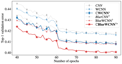
Validation and Test Accuracy. Top-1 accuracy of AlexNet-based models along training with ImageNet is plotted in Fig. 4. Similar plots are provided for ResNet in Fig. 10. In addition, error rates of AlexNet- and ResNet-based architectures, computed on the evaluation sets, are provided in Tab. 3 for ImageNet and Tab. 3 for CIFAR-10.

Our $\mathbb{C}$Mod-based approach significantly outperforms the baselines for AlexNet: $\mathbb{C}$WCNN vs WCNN (blue diamonds), and $\mathbb{C}$BlurWCNN vs BlurWCNN (red stars). Remarkably, the exclusive application of $\mathbb{C}$Mod-based antialiasing to the Gabor channels ($\mathbb{C}$WCNN, solid blue line) is sufficient to match the performance of blur-pooling-based antialiasing (BlurWCNN, dashed red line), which, in contrast, is implemented throughout the entire network. Positive results are also obtained for ResNet-based models trained on ImageNet (Tab. 3, bottom). However, adaptive blur pooling, when applied to the Gabor channels (ABlurWCNN), yields similar or marginally higher accuracy than our approach ($\mathbb{C}$ABlurWCNN). Nevertheless, our method is computationally more efficient, requires less memory (see “Computational Resources” below for more details), and do not demand additional training, unlike adaptive blur pooling. To better support this claim, we conducted ablation studies which we present in Sec. D.3. Finally, when trained on CIFAR-10 (see Tab. 3), our $\mathbb{C}$Mod-based antialiased models built upon ResNet-18 and 34 achieve significant gains in accuracy over non-antialiased models, as well as models antialiased with both blur-pooling-based methods.

As a side note, the training curves for WCNNs (colored dashed lines) closely follow those of standard CNNs (gray dotted lines). This is an expected result, since the former models are designed to mimic the behavior of the latter.

Shift Invariance (KL Divergence).

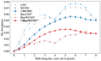
The mean KL divergence between outputs of shifted images are plotted in Fig. 5 for AlexNet trained on ImageNet. Moreover, the mean flip rate for shifted inputs (consistency) is reported in Tab. 3 for ImageNet (AlexNet and ResNet-34) and Tab. 3 for CIFAR-10 (ResNet-18 and 34).

In both AlexNet and WAlexNet, the initial convolution layer’s output undergoes a one-pixel shift for every four-pixel shift in the input image. Consequently, any divergence between the output vectors is due to the instability of subsequent layers to one-pixel shifts. In contrast, instabilities which are accountable to the initial layer are observed for shifts that are not multiples of $4$. Likewise, for input shifts of eight pixels, the max pooling’s output is shifted by exactly one pixel, resulting in even higher stability. In $\mathbb{C}$WAlexNet, the same eight-to-one-pixel ratio occurs to the modulus layer’s output, which explains why the two curves meet for $8$-pixel shifts. However, the $\mathbb{R}$Max-$\mathbb{C}$Mod substitution has greatly reduced first-layer instabilities, resulting in a flattened curve and avoiding the “bumps” observed for non-antialiased models.

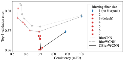
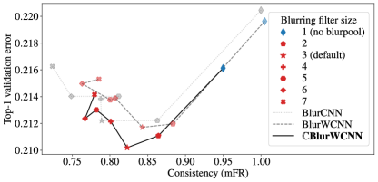
On the other hand, BlurAlexNet and BlurWAlexNet exhibit considerably flattened curves compared to non-antialiased models, as well as $\mathbb{C}$WAlexNet. This demonstrates the effectiveness of blur-pooling-based method in enhancing shift invariance. Applying $\mathbb{C}$Mod-based antialiasing instead of blur pooling on the Gabor channels ($\mathbb{C}$BlurWAlexNet) actually degrades shift invariance (except for shifts smaller than $1.5$ pixels), as evidenced by the bell-shaped curve. Nevertheless, the corresponding classifier is significantly more accurate. This is not surprising, as our approach prioritizes the conservation of high-frequency details, which are important for classification. An extreme reduction of shift variance using a large blur pooling filter would indeed result in a significant loss of accuracy. Therefore, our work achieves a better balance between shift invariance and information preservation. To gain further insights into this phenomenon, we conducted experiments by varying the size of the blurring filters in AlexNet-based models. Figure 6 shows the relationship between consistency and prediction accuracy on ImageNet (custom validation set), for different filter sizes ranging from $1$ (no blur pooling) to $7$ (heavy loss of high-frequency information). We find that a near-optimal trade-off is achieved when the filter size is set to $2$ or $3$. Furthermore, at equivalent consistency levels, $\mathbb{C}$BlurWCNN outperforms BlurWCNN in terms of accuracy. Note however that the optimal version of $\mathbb{C}$BlurWCNN is not more consistent than the optimal version of BlurWCNN, despite achieving higher accuracy.

Figure 6: Classification accuracy (ten-crops) vs consistency, measuring the stability of predictions to small input shifts, for AlexNet-based models (the lower the better for both axes). For each of the three architectures, we increased the blurring filter size from $1$ (i.e., no blur pooling) to $7$. The blue diamonds (no blur pooling) and red stars (blur pooling with filters of size $3$) correspond to the models from Figs. 4 and 5. At equivalent consistency levels, our $\mathbb{C}$Mod-based approach (solid line) yields higher accuracy.

Computational Resources.

Table 4 compares the computational resources and memory footprint required for each antialiasing method. To achieve this, we considered models with freely-trained convolutions, because the goal was to evaluate the computational performances of the various antialiasing approaches, excluding implementation tricks based on DT-$\mathbb{C}$WPT from the scope of analysis. More details are provided in Appendices F and G.

Method	Computational cost		Memory footprint
	AlexNet	ResNet	AlexNet	ResNet
No antialiasing (ref)	$\mathit{1.0}$	$\mathit{1.0}$	$\mathit{1.0}$	$\mathit{1.0}$
BlurPool [42]	$4.0$	$1.0$	$4.7$	$1.9$
ABlurPool [45]	–	$2.1$	–	$2.0$
$\mathbb{C}$Mod (ours)	$\mathbf{0.5}$	$\mathbf{0.5}$	$\mathbf{0.6}$	$\mathbf{0.4}$

Table 4: Computational cost and memory footprint required for each antialiasing method, per Gabor channel. The values are normalized relative to non-antialiased AlexNet or ResNet. Computational cost: FLOPs for computing $\mathrm{Y}^{\operatorname{max}}_{l}$ (11) or $\mathrm{Y}^{\operatorname{mod}}_{l}$ (13). Memory footprint: size of the intermediate and output tensors saved by PyTorch for the backward pass.

4 Conclusion

The mathematical twins introduced in this paper serve a proof of concept for our $\mathbb{C}$Mod-based antialiasing approach. However, its range of application extends well beyond DT-$\mathbb{C}$WPT filters. While we focused on the first convolution layer, it is important to note that such initial layers play a critical role in CNNs by extracting low-level geometric features such as edges, corners or textures. Therefore, a specific attention is required for their design. In contrast, deeper layers are more focused on capturing high-level structures that conventional image processing tools are poorly suited for, as pointed out by Oyallon et al. in the context of hybrid scattering networks [26].

Furthermore, while our approach is tailored for CNN architectures, which were chosen to make a fair comparison to related methods, it has potential for broader applicability. There is a growing interest in using self-attention mechanisms in computer vision [8] to capture complex, long-range dependencies among image representations. Recent work on vision transformers has proposed using the first layers of a CNN as a “convolutional token embedding” [10, 36, 39], effectively reintroducing inductive biases to the architecture, such as locality and weight sharing. By applying our antialiasing method to this embedding, we can provide self-attention modules with nearly shift-invariant inputs, which could be highly beneficial in improving the performance of vision transformers, especially when the amount of available data is limited.

Appendix A Design of WCNNs: Technical Details

In this section, we provide complements to the description of the mathematical twin (WCNN) introduced in Sec. 2.3. We explained that, for each Gabor channel $l\in\mathcal{G}$, the average kernel $\widetilde{\mathrm{V}}_{l}$ is the real part of a DT-$\mathbb{C}$WPT filter, as described in (18). We now explain how the filter selection is done; in other words, how $k^{\prime}$ is chosen among $\left\{1\mathinner{\ldotp\ldotp}4\times 4^{0}pt\right\}$. Since input images are real-valued, we restrict to the filters with bandwidth located in the half-plane of positive $x$-values. For the sake of concision, we denote by $K_{\operatorname{dt}}:=2\times 4^{0}pt$ the number of such filters.

For any RGB image $\mathbf{X}\in\mathcal{S}^{3}$, a luminance image $\mathrm{X}^{\operatorname{lum}}\in\mathcal{S}$ is computed following (17), using a $1\times 1$ convolution layer. Then, DT-$\mathbb{C}$WPT is performed on $\mathrm{X}^{\operatorname{lum}}$. We denote by $\mathbf{D}:=(\mathrm{D}_{k})_{k\in\left\{1\mathinner{\ldotp\ldotp}K_{\operatorname{dt}}\right\}}$ the tensor containing the real part of the DT-$\mathbb{C}$WPT feature maps:

$$\mathrm{D}_{k}=\bigl{(}\mathrm{X}^{\operatorname{lum}}\star\operatorname{Re}\mathrm{W}^{(0pt)}_{k}\bigr{)}\downarrow 2^{0pt-1}.$$ (23)

For the sake of computational efficiency, DT-$\mathbb{C}$WPT is performed with a succession of subsampled separable convolutions and linear combinations of real-valued wavelet packet feature maps [30]. To match the subsampling factor $m:=2^{0pt-1}$ of the standard model, the last decomposition stage is performed without subsampling.

Filter Selection.

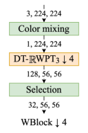
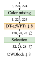
The number of dual-tree feature maps $K_{\operatorname{dt}}$ may be greater than the number of Gabor channels $L_{\operatorname{gabor}}$. In that case, we therefore want to select filters that contribute the most to the network’s predictive power. First, the low-frequency feature maps ${\mathrm{D}}_{0}$ and ${\mathrm{D}}_{(4^{0}pt+1)}$ are discarded. Then, a subset of $K_{\operatorname{dt}}^{\prime}<K_{\operatorname{dt}}$ feature maps is manually selected and permuted in order to form clusters in the Fourier domain. Considering a (truncated) permutation matrix $\boldsymbol{\varSigma}\in\mathbb{R}^{K_{\operatorname{dt}}^{\prime}\times K_{\operatorname{dt}}}$, the output of this transformation, denoted by $\mathbf{D}^{\prime}\in\mathcal{S}^{K_{\operatorname{dt}}^{\prime}}$, is defined by:

$$\mathbf{D}^{\prime}:=\boldsymbol{\varSigma}\,\mathbf{D}.$$ (24)

The feature maps $\mathbf{D}^{\prime}$ are then sliced into $Q$ groups of channels $\mathbf{D}^{(q)}\in\mathcal{S}^{K_{q}}$, each of them corresponding to a cluster of band-pass dual-tree filters with neighboring frequencies and orientations. On the other hand, the output of the wavelet block, $\mathbf{Y}^{\operatorname{gabor}}:=(\mathrm{Y}_{l})_{l\in\left\{L_{\operatorname{free}}+1\mathinner{\ldotp\ldotp}L\right\}}\in\mathcal{S}^{L_{\operatorname{gabor}}}$, where $\mathrm{Y}_{l}$ has been introduced in (6), is also sliced into $Q$ groups of channels $\mathbf{Y}^{(q)}\in\mathcal{S}^{L_{q}}$. Then, for each group $q\in\left\{1\mathinner{\ldotp\ldotp}Q\right\}$, an affine mapping between $\mathbf{D}^{(q)}$ and $\mathbf{Y}^{(q)}$ is performed. It is characterized by a trainable matrix $\boldsymbol{A}^{(q)}:=\bigl{(}\boldsymbol{\alpha}^{(q)}_{1},\,\cdots,\,\boldsymbol{\alpha}^{(q)}_{L_{q}}\bigr{)}^{\top}\in\mathbb{R}^{L_{q}\times K_{q}}$ such that, for any $l\in\left\{1\mathinner{\ldotp\ldotp}L_{q}\right\}$,

$$\mathrm{Y}^{(q)}_{l}:=\boldsymbol{\alpha}^{(q)\top}_{l}\cdot\mathbf{D}^{(q)}.$$ (25)

As in the color mixing stage, this operation is implemented as a $1\times 1$ convolution layer.

A schematic representation of the real- and complex-valued wavelet blocks can be found in Fig. 7.

Figure 7: Detail of a wavelet block with $0pt=3$ as in AlexNet, in its $\mathbb{R}$Max (left) and $\mathbb{C}$Mod (right) versions. DT-$\mathbb{R}$WPT corresponds to the real part of DT-$\mathbb{C}$WPT.

Sparse Regularization.

For any group $q\in\left\{1\mathinner{\ldotp\ldotp}Q\right\}$ and output channel $l\in\left\{1\mathinner{\ldotp\ldotp}L_{q}\right\}$, we want the model to select one and only one wavelet packet feature map within the $q$-th group. In other words, each row vector $\boldsymbol{\alpha}^{(q)}_{l}:=\bigl{(}\alpha^{(q)}_{l,\,1},\,\cdots,\,\alpha^{(q)}_{l,\,K_{q}}\bigr{)}^{\top}$ of $\boldsymbol{A}^{(q)}$ contains no more than one nonzero element, such that (25) becomes

$$\mathrm{Y}^{(q)}_{l}=\alpha^{(q)}_{lk}\mathrm{D}^{(q)}_{k}$$ (26)

for some (unknown) value of $k\in\left\{1\mathinner{\ldotp\ldotp}K_{q}\right\}$. To enforce this property during training, we add a mixed-norm $l^{1}/l^{\infty}$-regularizer [25] to the loss function to penalize non-sparse feature map mixing as follows:

$$\mathcal{L}:=\mathcal{L}_{0}+\sum_{q=1}^{Q}\lambda_{q}\sum_{l=1}^{L_{q}}\left(\frac{\bigl{\|}\boldsymbol{\alpha}^{(q)}_{l}\bigr{\|}_{1}}{\bigl{\|}\boldsymbol{\alpha}^{(q)}_{l}\bigr{\|}_{\infty}}-1\right),$$ (27)

where $\mathcal{L}_{0}$ denotes the standard cross-entropy loss and $\boldsymbol{\lambda}\in\mathbb{R}^{Q}$ denotes a vector of regularization hyperparameters. Note that the unit bias in (27) serves for interpretability of the regularized loss ($\mathcal{L}=\mathcal{L}_{0}$ in the desired configuration) but has no impact on training.

Appendix B Batch Normalization in ResNet

This section complements Sec. 2.5 in the main paper. In many recent architectures including ResNet, the bias (see Fig. 3(a)) is replaced by an affine batch normalization layer (BN). In this section, we show how to adapt our approach to this context.

(a) ResNet

(b) WResNet (baseline)

(c) $\mathbb{C}$WResNet (proposed approach)

Figure 8: First layers of ResNet and its variants, corresponding to a convolution layer followed by ReLU and max pooling. The models are framed according to the same colors and line styles as in Fig. 10. The bias module from Fig. 3(a) has been replaced by an affine batch normalization layer (“BN + Bias”, or “BN$0$ + Bias” when placed after Modulus—see Appendix B). Top: ResNet without blur pooling. Middle: Zhang’s “blurpooled” models [42]. Bottom: Zou et al.’s approach, using adaptive blur pooling [45].

 

A BN layer is parameterized by trainable weight and bias vectors, respectively denoted by $\boldsymbol{a}$ and $\boldsymbol{b}\in\mathbb{R}^{L}$. In the remaining of the section, we consider input images $\mathbf{X}$ as a stack of discrete stochastic processes. Then, expression (7) is replaced by

$$\mathrm{A}_{l}\!:=\!\operatorname{MaxPool}\!\left\{\operatorname{ReLU}\!\left(a_{l}\!\cdot\!\frac{\mathrm{Y}_{l}\!-\!\mathbb{E}_{m}[\mathrm{Y}_{l}]}{\sqrt{\mathbb{V}_{m}[\mathrm{Y}_{l}]\!+\!\varepsilon}}\!+\!b_{l}\right)\!\right\}\!,$$ (28)

with $\mathrm{Y}_{l}$ satisfying (6) (output of the first convolution layer). In the above expression, we have introduced $\mathbb{E}_{m}(\mathrm{Y}_{l})\in\mathbb{R}$ and $\mathbb{V}_{m}(\mathrm{Y}_{l})\in\mathbb{R}_{+}$, which respectively denote the mean expected value and variance of $\mathrm{Y}_{l}[\boldsymbol{n}]$, for indices $\boldsymbol{n}$ contained in the support of $\mathrm{Y}_{l}$, denoted by $\operatorname{supp}(\mathrm{Y}_{l})$. Let us denote by $N\in\mathbb{N}\setminus\{0\}$ the support size of input images. Therefore, if the filter’s support size $N_{\operatorname{filt}}$ is much smaller that $N$, then $\operatorname{supp}(\mathrm{Y}_{l})$ is roughly of size $N/m$. We thus define the above quantities as follows:

$$\mathbb{E}_{m}[\mathrm{Y}_{l}] :=\frac{m^{2}}{N^{2}}\sum_{\boldsymbol{n}\in\mathbb{Z}^{2}}\mathbb{E}[\mathrm{Y}_{l}[\boldsymbol{n}]];$$ (29)

$$\mathbb{V}_{m}[\mathrm{Y}_{l}] :=\frac{m^{2}}{N^{2}}\sum_{\boldsymbol{n}\in\mathbb{Z}^{2}}\mathbb{V}[\mathrm{Y}_{l}[\boldsymbol{n}]].$$ (30)

In practice, estimators are computed over a minibatch of images, hence the layer’s denomination. Besides, $\varepsilon>0$ is a small constant added to the denominator for numerical stability. For the sake of concision, we now assume that $\boldsymbol{a}=\boldsymbol{1}$. Extensions to other multiplicative factors is straightforward.

Let $l\in\mathcal{G}$ denote a Gabor channel. Then, recall that $\mathrm{Y}_{l}$ satisfies (19) (output of the WBlock), with

$$\widetilde{\mathrm{V}}_{l}:=\operatorname{Re}\widetilde{\mathrm{W}}_{l},$$ (31)

where $\widetilde{\mathrm{W}}_{l}$ denotes one of the Gabor-like filters spawned by DT-$\mathbb{C}$WPT. The following proposition states that, if the kernel’s bandwidth is small enough, then the output of the convolution layer sums to zero.

Proposition 1.

We assume that the Fourier transform of $\widetilde{\mathrm{W}}_{l}$ is supported in a region of size $\kappa\times\kappa$ which does not contain the origin (Gabor-like filter). If, moreover, $\kappa\leq\frac{2\pi}{m}$, then

$$\sum_{\boldsymbol{n}\in\mathbb{Z}^{2}}\mathrm{Y}_{l}[\boldsymbol{n}]=0.$$ (32)

Proof.

This proposition takes advantage of Shannon’s sampling theorem. A similar reasoning can be found in the proof of Theorem 1 in [23]. ∎

In practice, the power spectrum of DT-$\mathbb{C}$WPT filters cannot be exactly zero on regions with nonzero measure, since they are finitely supported. However, we can reasonably assume that it is concentrated within a region of size $\pi/2^{0pt-1}=\pi/m$, as explained in [23]. Therefore, since we have discarded low-pass filters, the conditions of Eq. 32 are approximately met for $\widetilde{\mathrm{W}}_{l}$.

We now assume that (32) is satisfied. Moreover, we assume that $\mathbb{E}[\mathrm{Y}_{l}[\boldsymbol{n}]]$ is constant for any $\boldsymbol{n}\in\operatorname{supp}(\mathrm{Y}_{l})$. Aside from boundary effects, this is true if $\mathbb{E}[\mathrm{X}^{\operatorname{lum}}[\boldsymbol{n}]]$ is constant for any $\boldsymbol{n}\in\operatorname{supp}(\mathrm{X}^{\operatorname{lum}})$. We then get, for any $\boldsymbol{n}\in\mathbb{Z}^{2}$, $\mathbb{E}[\mathrm{Y}_{l}[\boldsymbol{n}]]=0$. Therefore, interchanging max pooling and ReLU yields the normalized version of (10):

$$\mathrm{A}^{\operatorname{max}}_{l}=\operatorname{ReLU}\left(\frac{\mathrm{Y}^{\operatorname{max}}_{l}}{\sqrt{\mathbb{E}_{m}[\mathrm{Y}_{l}^{2}]+\varepsilon}}+b_{l}\right).$$ (33)

As in Sec. 2.2, we replace $\mathrm{Y}^{\operatorname{max}}_{l}$ by $\mathrm{Y}^{\operatorname{mod}}_{l}$ for any Gabor channel $l\in\mathcal{G}$, which yields the normalized version of (12):

$$\mathrm{A}^{\operatorname{mod}}_{l}:=\operatorname{ReLU}\left(\frac{\mathrm{Y}^{\operatorname{mod}}_{l}}{\sqrt{\mathbb{E}_{m}[\mathrm{Y}_{l}^{2}]+\varepsilon}}+b_{l}\right).$$ (34)

Implementing (34) as a deep learning architecture is cumbersome because $\mathrm{Y}_{l}$ needs to be explicitly computed and kept in memory, in addition to $\mathrm{Y}^{\operatorname{mod}}_{l}$. Instead, we want to express the second-order moment $\mathbb{E}_{m}[\mathrm{Y}_{l}^{2}]$ (in the denominator) as a function of $\mathrm{Y}^{\operatorname{mod}}_{l}$. To this end, we state the following proposition.

Proposition 2.

If we restrict the conditions of Eq. 32 to $\kappa\leq\pi/m$, we have

$$\left\|\mathrm{Y}_{l}\right\|_{2}^{2}=2\left\|\mathrm{Y}^{\operatorname{mod}}_{l}\right\|_{2}^{2}.$$ (35)

Proof.

This result, once again, takes advantage of Shannon’s sampling theorem. The proof of our Proposition 3 in [23] is based on similar arguments. ∎

As for Eq. 32, the conditions of Eq. 35 are approximately met. We therefore assume that (35) is satisfied, and (34) becomes

$$\mathrm{A}^{\operatorname{mod}}_{l}:=\operatorname{ReLU}\left(\frac{\mathrm{Y}^{\operatorname{mod}}_{l}}{\sqrt{\frac{1}{2}\mathbb{E}_{2m}[{\mathrm{Y}^{\operatorname{mod}}_{l}}^{2}]+\varepsilon}}+b_{l}\right).$$ (36)

In the case of ResNet, the bias layer (Bias) is therefore preceded by a batch normalization layer without mean centering satisfying (36), which we call BN$0$. The second-order moment of ${\mathrm{Y}^{\operatorname{mod}}_{l}}$ is computed on feature maps which are twice smaller than $\mathrm{Y}_{l}$ in both directions—hence the index “$2m$” in (36), which is the subsampling factor for the $\mathbb{C}$Mod operator.

Schematic representations of $\mathbb{R}$Max- and $\mathbb{C}$Mod-based $\mathbb{C}$WResNet are provided in Fig. 8(a).

Appendix C Experimental Settings

In this section, we provide further information that complements the experimental details presented in Secs. 3.1 and 1.

As explained in Sec. 2.3, the decomposition depth $0pt$ is chosen such that $m=2^{0pt-1}$ (subsampling factor). Since $m=4$ in AlexNet and $2$ in ResNet, we get $0pt=3$ and $2$, respectively. Therefore, the number of dual-tree filters $K_{\operatorname{dt}}:=2\times 4^{0}pt$ is equal to $128$ and $32$, respectively.

We then manually selected $K_{\operatorname{dt}}^{\prime}<K_{\operatorname{dt}}$ filters. In particular, we removed the two low-pass filters, which are outside the scope of our theoretical study. Besides, for computational reasons, in WAlexNet we removed $32$ “extremely” high-frequency filters which are clearly absent from the standard model (see Fig. 9(a)). Finally, in WResNet we removed the $14$ filters whose bandwidths outreach the boundaries of the Fourier domain $\left[-\pi,\,\pi\right]^{2}$ (see Fig. 9(b)). These filters indeed have a poorly-defined orientation, since a small fraction of their energy is located at the far end of the Fourier domain [2, see Fig. 1, “Proposed DT-$\mathbb{C}$WPT”]. Therefore, they somewhat exhibit a checkerboard pattern.

(a) WAlexNet ($0pt=3$)

(b) WResNet ($0pt=2$)

Figure 9: Mapping scheme from DT-$\mathbb{C}$WPT feature maps $\mathbf{D}\in\mathcal{S}^{K_{\operatorname{dt}}}$ to the wavelet block’s output $\mathbf{Y}^{\operatorname{gabor}}\in\mathcal{S}^{L_{\operatorname{gabor}}}$. Each wavelet feature map is symbolized by a small square in the Fourier domain, where its energy is mainly located. The gray areas show the feature maps which have been manually removed. Elsewhere, each group of feature maps $\mathbf{D}^{(q)}\in\mathcal{S}^{K_{q}}$ is symbolized by a dark frame—in (b), $K_{q}$ is always equal to $1$. For each group $q\in\left\{1\mathinner{\ldotp\ldotp}Q\right\}$, a number indicates how many output channels $L_{q}$ are assigned to it. The colored numbers in (a) refer to groups on which we have applied $l^{\infty}/l^{1}$-regularization. Note that, when inputs are real-valued, only the half-plane of positive $x$-values is considered.

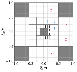
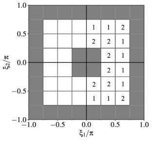
As explained in Appendix A, once the DT-$\mathbb{C}$WPT feature maps have been manually selected, the output $\mathbf{D}^{\prime}\in\mathcal{S}^{K_{\operatorname{dt}}^{\prime}}$ is sliced into $Q$ groups of channels $\mathbf{D}^{(q)}\in\mathcal{S}^{K_{q}}$. For each group $q$, a depthwise linear mapping from $\mathbf{D}^{(q)}$ to a bunch of output channels $\mathbf{Y}^{(q)}\in\mathcal{S}^{L_{q}}$ is performed. Finally, the wavelet block’s output feature maps $\mathbf{Y}^{\operatorname{gabor}}\in\mathcal{S}^{L_{\operatorname{gabor}}}$ are obtained by concatenating the outputs $\mathbf{Y}^{(q)}$ depthwise, for any $q\in\left\{1\mathinner{\ldotp\ldotp}Q\right\}$. Figure 9 shows how the above grouping is made, and how many output channels $L_{q}$ each group $q$ is assigned to.

During training, the above process aims at selecting one single DT-$\mathbb{C}$WPT feature map among each group. This is achieved through mixed-norm $l^{\infty}/l^{1}$ regularization, as introduced in (27). The regularization hyperparameters $\lambda_{q}$ have been chosen empirically. If they are too small, then regularization will not be effective. On the contrary, if they are too large, then the regularization term will become predominant, forcing the trainable parameter vector $\boldsymbol{\alpha}^{(q)}_{l}$ to randomly collapse to $0$ except for one element. The chosen values of $\lambda_{q}$ are displayed in Tab. 5.

Model	Filt. frequency	Reg. param.
WAlexNet	$\left[\pi/8,\,\pi/4\right[$	–
	$\left[\pi/4,\,\pi/2\right[$	$4.1\cdot 10^{-3}$
	$\left[\pi/2,\,\pi\right[$	$3.2\cdot 10^{-4}$
WResNet	any	–

Table 5: Regularization hyperparameters $\lambda_{q}$ for each group $q$ of DT-$\mathbb{C}$WPT feature maps. The groups with only one feature map do not need any regularization since this feature map is automatically selected. The second and third rows of WAlexNet correspond to the blue and magenta groups in Fig. 9(a), respectively.

Finally, the split $L_{\operatorname{free}}$-$L_{\operatorname{gabor}}$ between the freely-trained and Gabor channels, provided in the last row of Tab. 1 (main document), have been empirically determined from the standard models. More specifically, considering standard AlexNet and ResNet-34 trained on ImageNet (see Fig. 12), we determined the characteristics of each convolution kernel: frequency, orientation, and coherence index (which indicates whether an orientation is clearly defined). This was done by computing the tensor structure [16]. Then, by applying proper thresholds, we isolated the Gabor-like kernels from the others, yielding the approximate values of $L_{\operatorname{free}}$ and $L_{\operatorname{gabor}}$. Furthermore, this procedure allowed us to draw a rough estimate of the distribution of the Gabor-like filters in the Fourier domain, which was helpful to design the mapping scheme shown in Fig. 9.

Appendix D Additional Figures and Tables

D.1 Validation Error Along Training

As for AlexNet in Fig. 4, Top-1 validation curves of ResNet-based models along training with ImageNet and CIFAR-10 are plotted in Fig. 10. In many cases, accuracy increases when applying our $\mathbb{C}$Mod-based antialiasing method (dashed versus solid lines). However, in some cases, the gain on the validation set (a subset of images put aside from the training set) is marginal, for instance BlurWResNet-34 versus $\mathbb{C}$BlurWResNet-34 trained on ImageNet (Fig. 10(a), red stars), or non-existent, for instance WResNet-18 versus $\mathbb{C}$WResNet-18 trained on CIFAR-10 (Fig. 10(b), blue diamonds). Yet, notable gains are observed on the evaluation set (a separate dataset provided by ImageNet or CIFAR), as reported in Tabs. 3 and 3. This indicates a better generalization capability of our approach, compared to the static blur pooling-based method, or no antialiasing. In particular, for ImageNet classification (Tab. 3, bottom), simply replacing the blurpooled Gabor channels in the first layer with our $\mathbb{C}$Mod-based approach (BlurWCNN versus $\mathbb{C}$BlurWCNN) produces improvements on a similar order of magnitude as adaptive blur pooling, which is applied throughout the whole network (ABlurWCNN).

(a) ResNet-34, trained on ImageNet-1K

(b) ResNet-18, trained on CIFAR-10

(c) ResNet-34, trained on CIFAR-10

Figure 10: Evolution of the top-1 validation error (one-crop) along training, for ResNet-based models, as described in Fig. 8(a). The freely-trained models, upon which the mathematical twins are built, appear in faint gray. Legend: ^†static and ^‡adaptive blur pooling; ^∗$\mathbb{C}$Mod-based antialiasing (our approach).

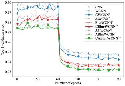
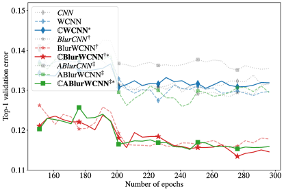
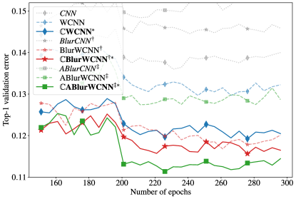
D.2 Accuracy vs Consistency

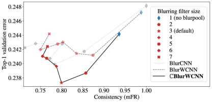
Figure 11 shows the relationship between consistency and prediction accuracy of AlexNet and ResNet-based models on ImageNet, for different filter sizes ranging from $1$ (no blur pooling) to $7$ (heavy loss of high-frequency information). The data for AlexNet on the validation set are displayed in the main document, Fig. 6. As recommended by Zhang [42], the optimal trade-off is generally achieved when the blurring filter size is equal to $3$. Moreover, in either case, at equivalent level of consistency, replacing blur pooling by our $\mathbb{C}$Mod-based antialiasing approach in the Gabor channels increases accuracy.

(a) AlexNet, test set ($50$K images)

(b) ResNet-34, validation set ($100$K images)

(c) ResNet-34, test set ($50$K images)

Figure 11: Classification accuracy (ten-crops) vs consistency, measuring the stability of predictions to small input shifts (the lower the better for both axes). The metrics have been computed on ImageNet-1K, on both validation set ($100$K images set aside from the training set) and test set ($50$K images provided as a separate dataset). For each model (BlurCNN, BlurWCNN and $\mathbb{C}$BlurWCNN), we increased the blurring filter size from $1$ (i.e., no blur pooling) to $7$. The blue diamonds (no blur pooling) and red stars (blur pooling with filters of size $3$) correspond to the models from Fig. 4 for AlexNet and Fig. 10(a) for ResNet (models trained after $90$ epochs).

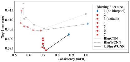
D.3 Ablation Study

In Sec. 3.3, we showed that our models outperform the baselines, except when adaptive blur pooling is used as an antialiasing method. In that case, although applying our $\mathbb{C}$Mod-based approach on the Gabor channels instead of adaptive blur pooling leads to slightly degraded accuracy, it comes with far less computational resources and memory footprint, as shown in Tab. 4. However, one may wonder: what happens if we do not employ any antialiasing on the Gabor channels (and keep on using blur pooling in the rest of the network)? Do we reach similar accuracy as well? To answer this question, we trained such ablated models, in both static and adaptive blur-pooling situations.

Model	One-crop		Ten-crops		Shifts
	top-1	top-5	top-1	top-5	mFR
WCNN◆	27.4	9.2	24.7	7.6	77.2
BlurWCNN†	26.7	8.6	24.1	7.3	65.2
$\mathbb{C}$BlurWCNN†∗	26.5	8.4	23.7	7.0	62.5
$\boldsymbol{\to}$ BlurWCNN†◆	26.8	8.6	24.3	7.1	69.7
ABlurWCNN‡	26.0	8.2	23.6	6.9	62.1
$\mathbb{C}$ABlurWCNN‡∗	26.1	8.2	23.7	7.0	63.1
$\boldsymbol{\to}$ ABlurWCNN†◆	26.4	8.4	23.9	7.0	70.3

Table 6: Ablation study on WResNet. Evaluation metrics on ImageNet (%): the lower the better. Models: ^†static and ^‡adaptive blur pooling; ^∗$\mathbb{C}$Mod-based antialiasing on the Gabor channels (our approach); ^◆ablated model: no antialiasing on the Gabor channels (neither blur pooling nor $\mathbb{C}$Mod); ^◆no antialiasing anywhere.

We found that removing antialiasing from the Gabor channels (either blur pooling or $\mathbb{C}$Mod) generally leads to decreased accuracy and consistency, as shown in Tab. 6. However, when using adaptive blur pooling, the primary improvements in performance come from other parts of the network—as evidenced when comparing the first and last rows. This limits the influence of antialiasing on the Gabor channels. Yet, although adaptive blur pooling yields the most important gains in performance, it comes at a substantial increase in computational resources due to the need for multiple such antialiasing layers throughout the network.

Appendix E Kernel Visualization (Standard Models)

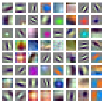
The convolution kernels $\mathbf{V}:=(\mathrm{V}_{lk})_{l\in\left\{1\mathinner{\ldotp\ldotp}64\right\},\,k\in\left\{1\mathinner{\ldotp\ldotp}3\right\}}\in\mathcal{S}^{64\times 3}$ satisfying (11) are shown in Fig. 12 for freely-trained AlexNet and ResNet-34 trained on ImageNet. The kernels are shown as RGB color images. When comparing them with WCNN kernels in Fig. 2, we can notice that, up to a few exceptions, the freely-trained channels ($4$ and $5$ first rows for AlexNet and ResNet, respectively) have been specialized to lower-frequency filters (mono- or bi-color blobs).

(a) AlexNet

(b) ResNet

Figure 12: Convolution kernels in the first layer of freely-trained AlexNet (a) and ResNet-34 (b), after training with ImageNet-1K. For each output channel $l\in\left\{1\mathinner{\ldotp\ldotp}64\right\}$, the corresponding convolution kernel $(\mathrm{V}_{lk})_{k\in\left\{1\mathinner{\ldotp\ldotp}3\right\}}$ is displayed as an RGB image in the spatial domain (left), and its associated magnitude spectrum in the Fourier domain (right).

Appendix F Computational Cost

This section provides technical details about our estimation of the computational cost (FLOPs), such as reported in Tab. 4, for one input image and one Gabor channel. This metric was estimated in the case of standard 2D convolutions.

F.1 Average Computation Time per Operation

The estimated computation time for each type of operation has been reported in Tab. 7.

$$t_{\operatorname{s}} =1.0$$ (addition)

$$t_{\operatorname{p}} =1.0$$ (multiplication)

$$t_{\operatorname{e}} =0.75$$ (exponential)

$$t_{\operatorname{mod}} =3.5$$ (modulus)

$$t_{\operatorname{relu}} =0.75$$ (ReLU)

$$t_{\operatorname{max}} =12.0$$ (max pooling)

Table 7: Computation time per operation, determined experimentally using PyTorch (CPU computations). They have been normalized with respect to the computation time of an addition.

F.2 Computational Cost per Layer

In the following paragraphs, $L\in\mathbb{N}\setminus\{0\}$ denotes the number of output channels (depth) and $N^{\prime}\in\mathbb{N}\setminus\{0\}$ denotes the size of output feature maps (height and width). However, note that $N^{\prime}$ is not necessary the same for all layers. For instance, in standard ResNet, the output of the first convolution layer is of size $N^{\prime}=112$, whereas the output of the subsequent max pooling layer is of size $N^{\prime}=56$. For each type of layer, we calculate the number of FLOPs required to produce a single output channel $l\in\left\{1\mathinner{\ldotp\ldotp}L\right\}$. Moreover, we assume, without loss of generality, that the model processes one input image at a time.

Convolution Layers.

Inputs of size $(K\times N\times N)$ (input channels, height and width); outputs of size $(L\times N^{\prime}\times N^{\prime})$. For each output unit, a convolution layer with kernels of size $(N_{\operatorname{filt}}\times N_{\operatorname{filt}})$ requires $KN_{\operatorname{filt}}^{2}$ multiplications and $KN_{\operatorname{filt}}^{2}-1$ additions. Therefore, the computational cost per output channel is equal to

$$T_{\operatorname{conv}}={N^{\prime}}^{2}\left((KN_{\operatorname{filt}}^{2}-1)\cdot t_{\operatorname{s}}+KN_{\operatorname{filt}}^{2}\cdot t_{\operatorname{p}}\right).$$ (37)

Complex Convolution Layers.

Inputs of size $(K\times N\times N)$; complex-valued outputs of size $(L\times N^{\prime}\times N^{\prime})$. For each output unit, a complex-valued convolution layer requires $2\times KN_{\operatorname{filt}}^{2}$ multiplications and $2\times(KN_{\operatorname{filt}}^{2}-1)$ additions. Computational cost per output channel:

$$T_{\mathbb{C}\operatorname{conv}}=2{N^{\prime}}^{2}\left((KN_{\operatorname{filt}}^{2}-1)\cdot t_{\operatorname{s}}+KN_{\operatorname{filt}}^{2}\cdot t_{\operatorname{p}}\right).$$ (38)

Note that, in our implementations, the complex-valued convolution layers are less expensive than the real-valued ones, because the output size $N^{\prime}$ is twice smaller, due to the larger subsampling factor.

Bias and ReLU.

Inputs and outputs of size $(L\times N^{\prime}\times N^{\prime})$. One evaluation for each output unit:

$$T_{\operatorname{bias}}={N^{\prime}}^{2}\,t_{\operatorname{s}}\qquad\mbox{and}\qquad T_{\operatorname{relu}}={N^{\prime}}^{2}\,t_{\operatorname{relu}}.$$ (39)

Max Pooling.

Outputs of size $(L\times N^{\prime}\times N^{\prime})$, with $N^{\prime}$ depending on whether subsampling is performed at this stage (no subsampling when followed by a blur pooling layer). One evaluation for each output unit:

$$T_{\operatorname{max}}={N^{\prime}}^{2}\,t_{\operatorname{max}}.$$ (40)

Modulus Pooling.

Complex-valued inputs and real-valued outputs of size $(L\times N^{\prime}\times N^{\prime})$. One evaluation for each output unit:

$$T_{\operatorname{mod}}={N^{\prime}}^{2}\,t_{\operatorname{mod}}.$$ (41)

Batch Normalization.

Inputs and outputs of size $(L\times N^{\prime}\times N^{\prime})$. A batch normalization (BN) layer, described in (28), can be split into several stages.

1. Mean: ${N^{\prime}}^{2}$ additions.

2. Standard deviation: ${N^{\prime}}^{2}$ multiplications, ${N^{\prime}}^{2}$ additions (second moment), ${N^{\prime}}^{2}$ additions (subtract squared mean).

3. Final value: ${N^{\prime}}^{2}$ additions (subtract mean), $2{N^{\prime}}^{2}$ multiplications (divide by standard deviation and multiplicative coefficient).

Overall, the computational cost per image and output channel of a BN layer is equal to

$$T_{\operatorname{bn}}={N^{\prime}}^{2}\left(4\,t_{\operatorname{s}}+3\,t_{\operatorname{p}}\right).$$ (42)

Static Blur Pooling.

Inputs of size $(L\times 2N^{\prime}\times 2N^{\prime})$; outputs of size $(L\times N^{\prime}\times N^{\prime})$. For each output unit, a static blur pooling layer [42] with filters of size $(N_{\operatorname{b}}\times N_{\operatorname{b}})$ requires $N_{\operatorname{b}}^{2}$ multiplications and $N_{\operatorname{b}}^{2}-1$ additions. The computational cost per output channel is therfore equal to

$$T_{\operatorname{blur}}={N^{\prime}}^{2}\left((N_{\operatorname{b}}^{2}-1)\cdot t_{\operatorname{s}}+N_{\operatorname{b}}^{2}\cdot t_{\operatorname{p}}\right).$$ (43)

Adaptive Blur Pooling.

Inputs of size $(L\times 2N^{\prime}\times 2N^{\prime})$; outputs of size $(L\times N^{\prime}\times N^{\prime})$. An adaptive blur pooling layer [45] with filters of size $(N_{\operatorname{b}}\times N_{\operatorname{b}})$ splits the $L$ output channels into $Q:=L/L_{\operatorname{g}}$ groups of $L_{\operatorname{g}}$ channels that share the same blurring filters. The adaptive blur pooling layer can be decomposed into the following stages.

1. Generation of blurring filters using a convolution layer with trainable kernels of size $(N_{\operatorname{b}}\times N_{\operatorname{b}})$: inputs of size $(L\times 2N^{\prime}\times 2N^{\prime})$, outputs of size $(QN_{\operatorname{b}}^{2}\times N^{\prime}\times N^{\prime})$. For each output unit, this stage requires $LN_{\operatorname{b}}^{2}$ multiplications and $LN_{\operatorname{b}}^{2}-1$ additions. The computational cost divided by the number $L$ of channels is therefore equal to

   $$T_{\operatorname{conv}\operatorname{ablur}}={N^{\prime}}^{2}\,\frac{N_{\operatorname{b}}^{2}}{L_{\operatorname{g}}}\times\\ \left((LN_{\operatorname{b}}^{2}-1)\cdot t_{\operatorname{s}}+LN_{\operatorname{b}}^{2}\cdot t_{\operatorname{p}}\right).$$ (44)

   Note that, despite being expressed on a per-channel basis, the above computational cost depends on the number $L$ of output channels. This is due to the asymptotic complexity of this stage in $O(L^{2})$.

2. Batch normalization, inputs and outputs of size $(QN_{\operatorname{b}}^{2}\times N^{\prime}\times N^{\prime})$:

   $$T_{\operatorname{bn}\operatorname{ablur}}={N^{\prime}}^{2}\,\frac{N_{\operatorname{b}}^{2}}{L_{\operatorname{g}}}\left(4\,t_{\operatorname{s}}+3\,t_{\operatorname{p}}\right).$$ (45)

3. Softmax along the depthwise dimension:

   $$T_{\operatorname{sftmx}\operatorname{ablur}}={N^{\prime}}^{2}\,\frac{N_{\operatorname{b}}^{2}}{L_{\operatorname{g}}}(t_{\operatorname{e}}+t_{\operatorname{s}}+t_{\operatorname{p}}).$$ (46)

4. Blur pooling of input feature maps, using the filter generated at stages (1)–(3): inputs of size $(L\times 2N^{\prime}\times 2N^{\prime})$, outputs of size $(L\times N^{\prime}\times N^{\prime})$. The computational cost per output channel is identical to the static blur pooling layer, even though the weights may vary across channels and spatial locations:

   $$T_{\operatorname{blur}}={N^{\prime}}^{2}\left((N_{\operatorname{b}}^{2}-1)\cdot t_{\operatorname{s}}+N_{\operatorname{b}}^{2}\cdot t_{\operatorname{p}}\right).$$ (47)

Overall, the computational cost of an adaptive blur pooling layer per input image and output channel is equal to

$$T_{\operatorname{ablur}}={N^{\prime}}^{2}\,\frac{N_{\operatorname{b}}^{2}}{L_{\operatorname{g}}}\left[\left((L+1)N_{\operatorname{b}}^{2}+3\right)\cdot t_{\operatorname{s}}\right.\\ \left.+\left((L+1)N_{\operatorname{b}}^{2}+4\right)\cdot t_{\operatorname{p}}+t_{\operatorname{e}}\right].$$ (48)

We notice that an adaptive blur pooling layer has an asymptotic complexity in $O(N_{\operatorname{b}}^{4})$, versus $O(N_{\operatorname{b}}^{2})$ for static blur pooling.

F.3 Application to AlexNet- and ResNet-based Models

Since they are normalized by the computational cost of standard models, the FLOPs reported in Tab. 4 only depend on the size of the convolution kernels and blur pooling filters, respectively denoted by $N_{\operatorname{filt}}$ and $N_{\operatorname{b}}\in\mathbb{N}\setminus\{0\}$. In addition, the computational cost of the adaptive blur pooling layer depend on the number of output channels $L$ as well as the number of output channels per group $L_{\operatorname{g}}$.

In practice, $N_{\operatorname{filt}}$ is respectively equal to $11$ and $7$ for AlexNet- and ResNet-based models. Moreover, $N_{\operatorname{b}}=3$, $L=64$ and $L_{\operatorname{g}}=8$. Actually, the computational cost is largely determined by the convolution layers, including step (1) of adaptive blur pooling.

Appendix G Memory Footprint

This section provides technical details about our estimation of the memory footprint for one input image and one output channel, such as reported in Tab. 4. This metric is generally difficult to estimate, and is very implementation-dependent. Hereafter, we consider the size of the output tensors, as well as intermediate tensors saved by torch.autograd for the backward pass. However, we didn’t take into account the tensors containing the trainable parameters. To get the size of intermediate tensors, we used the Python package PyTorchViz. These tensors are saved according to the following rules.

• Convolution (Conv), batch normalization (BN), Bias, max pooling (MaxPool or Max), blur pooling (BlurPool), and Modulus: the input tensors are saved, not the output. When Bias follows Conv or BN, no intermediate tensor is saved.

• ReLU, Softmax: the output tensors are saved, not the input.

• If an intermediate tensor is saved at both the output of a layer and the input of the next layer, its memory is not duplicated. An exception is Modulus, which stores the input feature maps as complex numbers.

• MaxPool or Max: a tensor of indices is kept in memory, indicating the position of the maximum values. The tensors are stored as 64-bit integers, so they weight twice as much as conventional float-32 tensors.

• BN: four 1D tensors of length $L$ are kept in memory: computed mean and variance, and running mean and variance. For BN0 (see Appendix B), where variance is not computed, only two tensors are kept in memory.

In the following paragraphs, we denote by $L$ the number of output channels, $N$ the size of input images (height and width), $m$ the subsampling factor of the baseline models ($4$ for AlexNet, $2$ for ResNet), $N_{\operatorname{b}}$ the blurring filter size (set to $3$ in practice). For each model, a table contains the size of all saved intermediate or output tensors. For example, the values associated to “Layer1 $\to$ Layer2” correspond to the depth (number of channel), height and width of the intermediate tensor between Layer1 and Layer2.

G.1 AlexNet-based Models

No Antialiasing.

$\mbox{Conv}\to\mbox{Bias}\to\mbox{ReLU}\to\mbox{MaxPool}$.

ReLU $\to$ MaxPool	$L$	$\frac{N}{m}$	$\frac{N}{m}$
MaxPool $\to$ output	$L$	$\frac{N}{2m}$	$\frac{N}{2m}$
MaxPool indices ($\times 2$)	$L$	$\frac{N}{2m}$	$\frac{N}{2m}$

Then, the memory footprint for each output channel is equal to

$$\implies S_{\operatorname{std}}=\frac{7}{4}\frac{N^{2}}{m^{2}}.$$

Static Blur Pooling.

$\mbox{Conv}\to\mbox{Bias}\to\mbox{ReLU}\to\mbox{BlurPool}\to\mbox{Max}\to\mbox{BlurPool}$.

ReLU $\to$ BlurPool	$L$	$\frac{2N}{m}$	$\frac{2N}{m}$
BlurPool $\to$ Max	$L$	$\frac{N}{m}$	$\frac{N}{m}$
Max $\to$ BlurPool	$L$	$\frac{N}{m}$	$\frac{N}{m}$
Max indices ($\times 2$)	$L$	$\frac{N}{m}$	$\frac{N}{m}$
BlurPool $\to$ output	$L$	$\frac{N}{2m}$	$\frac{N}{2m}$

$$\implies S_{\operatorname{blur}}=\frac{33}{4}\frac{N^{2}}{m^{2}}.$$

$\mathbb{C}$Mod-based Approach.

$\mathbb{C}\mbox{Conv}\to\mbox{Modulus}\to\mbox{Bias}\to\mbox{ReLU}$.

$\mathbb{C}$Conv $\to$ Modulus	$2L$	$\frac{N}{2m}$	$\frac{N}{2m}$
Modulus $\to$ Bias	$L$	$\frac{N}{2m}$	$\frac{N}{2m}$
ReLU $\to$ output	$L$	$\frac{N}{2m}$	$\frac{N}{2m}$

$$\implies S_{\operatorname{mod}}=\frac{N^{2}}{m^{2}}.$$

G.2 ResNet-based Models

No Antialiasing.

$\mbox{Conv}\to\mbox{BN}\to\mbox{Bias}\to\mbox{ReLU}\to\mbox{MaxPool}$.

Conv $\to$ BN	$L$	$\frac{N}{m}$	$\frac{N}{m}$
BN metrics	$4L$	–	–
ReLU $\to$ MaxPool	$L$	$\frac{N}{m}$	$\frac{N}{m}$
MaxPool $\to$ output	$L$	$\frac{N}{2m}$	$\frac{N}{2m}$
MaxPool indices ($\times 2$)	$L$	$\frac{N}{2m}$	$\frac{N}{2m}$

$$\implies S_{\operatorname{std}}=\frac{11}{4}\frac{N^{2}}{m^{2}}+4\approx\frac{11}{4}\frac{N^{2}}{m^{2}}.$$

Static Blur Pooling.

$\mbox{Conv}\to\mbox{BN}\to\mbox{Bias}\to\mbox{ReLU}\to\mbox{Max}\to\mbox{BlurPool}$.

Conv $\to$ BN	$L$	$\frac{N}{m}$	$\frac{N}{m}$
BN metrics	$4L$	–	–
ReLU $\to$ Max	$L$	$\frac{N}{m}$	$\frac{N}{m}$
Max $\to$ BlurPool	$L$	$\frac{N}{m}$	$\frac{N}{m}$
Max indices ($\times 2$)	$L$	$\frac{N}{m}$	$\frac{N}{m}$
BlurPool $\to$ output	$L$	$\frac{N}{2m}$	$\frac{N}{2m}$

$$\implies S_{\operatorname{blur}}=\frac{21}{4}\frac{N^{2}}{m^{2}}+4\approx\frac{21}{4}\frac{N^{2}}{m^{2}}.$$

Adaptive Blur Pooling.

$\mbox{Conv}\to\mbox{BN}\to\mbox{Bias}\to\mbox{ReLU}\to\mbox{Max}\to\mbox{ABlurPool}$.

Conv $\to$ BN	$L$	$\frac{N}{m}$	$\frac{N}{m}$
BN metrics	$4L$	–	–
ReLU $\to$ Max	$L$	$\frac{N}{m}$	$\frac{N}{m}$
Max $\to$ ABlurPool	$L$	$\frac{N}{m}$	$\frac{N}{m}$
Max indices ($\times 2$)	$L$	$\frac{N}{m}$	$\frac{N}{m}$
ABlurPool $\to$ output	$L$	$\frac{N}{2m}$	$\frac{N}{2m}$
Generate adaptive blurring filter
$\mbox{Conv}\to\mbox{BN}\to\mbox{Bias}\to\mbox{Softmax}$
Conv $\to$ BN	$\frac{LN_{\operatorname{b}}^{2}}{L_{\operatorname{g}}}$	$\frac{N}{2m}$	$\frac{N}{2m}$
BN metrics	$4\frac{LN_{\operatorname{b}}^{2}}{L_{\operatorname{g}}}$	–	–
Softmax $\to$ output	$\frac{LN_{\operatorname{b}}^{2}}{L_{\operatorname{g}}}$	$\frac{N}{2m}$	$\frac{N}{2m}$

$$\implies S_{\operatorname{ablur}} =\frac{21}{4}\frac{N^{2}}{m^{2}}+4+\frac{N_{\operatorname{b}}^{2}}{L_{\operatorname{g}}}\left(\frac{N^{2}}{2m^{2}}+4\right)$$

$$\approx\frac{21}{4}\frac{N^{2}}{m^{2}}+\frac{N_{\operatorname{b}}^{2}}{L_{\operatorname{g}}}\frac{N^{2}}{2m^{2}}.$$

$\mathbb{C}$Mod-based Approach.

$\mathbb{C}\mbox{Conv}\to\mbox{Modulus}\to\mbox{BN}0\to\mbox{Bias}\to\mbox{ReLU}$.

$\mathbb{C}\mbox{Conv}\to\mbox{Modulus}$	$2L$	$\frac{N}{2m}$	$\frac{N}{2m}$
$\mbox{Modulus}\to\mbox{BN}0$	$L$	$\frac{N}{2m}$	$\frac{N}{2m}$
BN0 metrics	$2L$	–	–
$\mbox{ReLU}\to$ output	$L$	$\frac{N}{2m}$	$\frac{N}{2m}$

$$\implies S_{\operatorname{mod}}=\frac{N^{2}}{m^{2}}+2\approx\frac{N^{2}}{m^{2}}.$$

References

- [1] Aharon Azulay and Yair Weiss. Why do deep convolutional networks generalize so poorly to small image transformations? Journal of Machine Learning Research, 20(184):1–25, 2019.
- [2] Ilker Bayram and Ivan W. Selesnick. On the Dual-Tree Complex Wavelet Packet and M-Band Transforms. IEEE Transactions on Signal Processing, 56(6):2298–2310, June 2008.
- [3] Christopher M. Bishop and Tom M. Mitchell. Pattern Recognition and Machine Learning. Springer, 2014.
- [4] Joan Bruna and Stéphane Mallat. Invariant Scattering Convolution Networks. IEEE Transactions on Pattern Analysis and Machine Intelligence, 35(8):1872–1886, May 2013.
- [5] Anadi Chaman and Ivan Dokmanic. Truly Shift-Invariant Convolutional Neural Networks. In Proc. IEEE/CVF Conference on Computer Vision and Pattern Recognition, pages 3773–3783, 2021.
- [6] Fergal Cotter and Nick Kingsbury. A Learnable Scatternet: Locally Invariant Convolutional Layers. In Proc. IEEE International Conference on Image Processing (ICIP), pages 350–354, Sept. 2019.
- [7] Muneer Ahmad Dedmari, Sailesh Conjeti, Santiago Estrada, Phillip Ehses, Tony Stöcker, and Martin Reuter. Complex Fully Convolutional Neural Networks for MR Image Reconstruction. In Florian Knoll, Andreas Maier, and Daniel Rueckert, editors, Machine Learning for Medical Image Reconstruction, Lecture Notes in Computer Science, pages 30–38, Cham, 2018. Springer International Publishing.
- [8] Alexey Dosovitskiy, Lucas Beyer, Alexander Kolesnikov, Dirk Weissenborn, Xiaohua Zhai, Thomas Unterthiner, Mostafa Dehghani, Matthias Minderer, Georg Heigold, Sylvain Gelly, Jakob Uszkoreit, and Neil Houlsby. An Image is Worth 16x16 Words: Transformers for Image Recognition at Scale. In Proc. International Conference on Learning Representations, 2021.
- [9] Shanel Gauthier, Benjamin Thérien, Laurent Alsène-Racicot, Muawiz Chaudhary, Irina Rish, Eugene Belilovsky, Michael Eickenberg, and Guy Wolf. Parametric Scattering Networks. In Proc. IEEE/CVF Conference on Computer Vision and Pattern Recognition, pages 5749–5758, 2022.
- [10] Ali Hassani, Steven Walton, Nikhil Shah, Abulikemu Abuduweili, Jiachen Li, and Humphrey Shi. Escaping the Big Data Paradigm with Compact Transformers. arXiv:2104.05704, June 2022.
- [11] J.P. Havlicek, J.W. Havlicek, and A.C. Bovik. The analytic image. In Proc. International Conference on Image Processing, volume 2, pages 446–449 vol.2, Oct. 1997.
- [12] Kaiming He, Xiangyu Zhang, Shaoqing Ren, and Jian Sun. Deep residual learning for image recognition. In Proc. IEEE Computer Society Conference on Computer Vision and Pattern Recognition, 2016.
- [13] Dan Hendrycks and Thomas Dietterich. Benchmarking Neural Network Robustness to Common Corruptions and Perturbations. In Proc. International Conference on Learning Representations, Mar. 2019.
- [14] Sergey Ioffe and Christian Szegedy. Batch Normalization: Accelerating Deep Network Training by Reducing Internal Covariate Shift. In Proc. 32nd International Conference on Machine Learning, pages 448–456. PMLR, June 2015.
- [15] Md Amirul Islam, Sen Jia, and Neil D. B. Bruce. How Much Position Information Do Convolutional Neural Networks Encode? In Proc. International Conference on Learning Representations, Jan. 2020.
- [16] Bernd Jahne. Practical Handbook on Image Processing for Scientific and Technical Applications. CRC Press, 2004.
- [17] Osman Semih Kayhan and Jan C. van Gemert. On Translation Invariance in CNNs: Convolutional Layers Can Exploit Absolute Spatial Location. In Proc. IEEE/CVF Conference on Computer Vision and Pattern Recognition, pages 14274–14285, 2020.
- [18] Nick Kingsbury. Design of Q-shift complex wavelets for image processing using frequency domain energy minimization. In Proceedings International Conference on Image Processing, volume 1, pages I–1013, 2003.
- [19] Nick Kingsbury and Julian Magarey. Wavelet Transforms in Image Processing. In Ales Procházka, Jan Uhlíř, P. W. J. Rayner, and N. G. Kingsbury, editors, Signal Analysis and Prediction, Applied and Numerical Harmonic Analysis, pages 27–46. Birkhäuser, Boston, MA, 1998.
- [20] Alex Krizhevsky, Ilya Sutskever, and Geoffrey E. Hinton. ImageNet classification with deep convolutional neural networks. Communications of the ACM, 60(6):84–90, May 2017.
- [21] Yann LeCun, Yoshua Bengio, and Geoffrey Hinton. Deep learning. Nature, 521(7553):436–444, 2015.
- [22] ChiYan Lee, Hideyuki Hasegawa, and Shangce Gao. Complex-Valued Neural Networks: A Comprehensive Survey. IEEE/CAA Journal of Automatica Sinica, 9(8):1406–1426, Aug. 2022.
- [23] Hubert Leterme, Kévin Polisano, Valérie Perrier, and Karteek Alahari. On the Shift Invariance of Max Pooling Feature Maps in Convolutional Neural Networks. arXiv:2209.11740, Sept. 2022.
- [24] Min Lin, Qiang Chen, and Shuicheng Yan. Network In Network. arXiv:1312.4400 [cs], 2014.
- [25] Jun Liu and Jieping Ye. Efficient L1/Lq Norm Regularization. arXiv:1009.4766, Sept. 2010.
- [26] Edouard Oyallon, Eugene Belilovsky, and Sergey Zagoruyko. Scaling the Scattering Transform: Deep Hybrid Networks. In Proc. IEEE International Conference on Computer Vision, pages 5618–5627, 2017.
- [27] Edouard Oyallon and Stéphane Mallat. Deep Roto-Translation Scattering for Object Classification. In Proc. IEEE Conference on Computer Vision and Pattern Recognition, pages 2865–2873, 2015.
- [28] Adam Paszke, Sam Gross, Soumith Chintala, Gregory Chanan, Edward Yang, Zachary DeVito, Zeming Lin, Alban Desmaison, Luca Antiga, and Adam Lerer. Automatic differentiation in PyTorch. Oct. 2017.
- [29] Olga Russakovsky, Jia Deng, Hao Su, Jonathan Krause, Sanjeev Satheesh, Sean Ma, Zhiheng Huang, Andrej Karpathy, Aditya Khosla, Michael Bernstein, Alexander C. Berg, and Li Fei-Fei. ImageNet Large Scale Visual Recognition Challenge. International Journal of Computer Vision, 115(3):211–252, Apr. 2015.
- [30] Ivan W. Selesnick, Richard Baraniuk, and Nick Kingsbury. The dual-tree complex wavelet transform. IEEE Signal Processing Magazine, 22(6):123–151, Nov. 2005.
- [31] Amarjot Singh and Nick Kingsbury. Dual-Tree wavelet scattering network with parametric log transformation for object classification. In ICASSP, IEEE International Conference on Acoustics, Speech and Signal Processing - Proceedings, 2017.
- [32] Antonio Torralba and Aude Oliva. Statistics of natural image categories. Network: Computation in Neural Systems, 14(3):391–412, Jan. 2003.
- [33] Chiheb Trabelsi, Olexa Bilaniuk, Ying Zhang, Dmitriy Serdyuk, Sandeep Subramanian, João Felipe Santos, Soroush Mehri, Negar Rostamzadeh, Yoshua Bengio, and Christopher J. Pal. Deep Complex Networks. In International Conference on Learning Representations, Feb. 2018.
- [34] Mark Tygert, Joan Bruna, Soumith Chintala, Yann LeCun, Serkan Piantino, and Arthur Szlam. A Mathematical Motivation for Complex-Valued Convolutional Networks. Neural Computation, 28(5):815–825, May 2016.
- [35] Thomas Wiatowski and Helmut Bölcskei. A Mathematical Theory of Deep Convolutional Neural Networks for Feature Extraction. IEEE Transactions on Information Theory, 64(3):1845–1866, Mar. 2018.
- [36] Haiping Wu, Bin Xiao, Noel Codella, Mengchen Liu, Xiyang Dai, Lu Yuan, and Lei Zhang. CvT: Introducing Convolutions to Vision Transformers. In Proc. IEEE/CVF International Conference on Computer Vision, pages 22–31, 2021.
- [37] Jin Xu, Hyunjik Kim, Thomas Rainforth, and Yee Teh. Group Equivariant Subsampling. In Advances in Neural Information Processing Systems, volume 34, pages 5934–5946, 2021.
- [38] Jason Yosinski, Jeff Clune, Yoshua Bengio, and Hod Lipson. How transferable are features in deep neural networks? In Advances in Neural Information Processing Systems, pages 3320–3328, 2014.
- [39] Kun Yuan, Shaopeng Guo, Ziwei Liu, Aojun Zhou, Fengwei Yu, and Wei Wu. Incorporating Convolution Designs Into Visual Transformers. In Proc. IEEE/CVF International Conference on Computer Vision, pages 579–588, 2021.
- [40] John Zarka, Louis Thiry, Tomás Angles, and Stéphane Mallat. Deep Network Classification by Scattering and Homotopy Dictionary Learning. In International Conference on Learning Representations, 2020.
- [41] Matthew D. Zeiler and Rob Fergus. Visualizing and understanding convolutional networks. In Lecture Notes in Computer Science (Including Subseries Lecture Notes in Artificial Intelligence and Lecture Notes in Bioinformatics), 2014.
- [42] Richard Zhang. Making Convolutional Networks Shift-Invariant Again. In International Conference on Machine Learning, pages 7324–7334. PMLR, May 2019.
- [43] Zhimian Zhang, Haipeng Wang, Feng Xu, and Ya-Qiu Jin. Complex-Valued Convolutional Neural Network and Its Application in Polarimetric SAR Image Classification. IEEE Transactions on Geoscience and Remote Sensing, 55(12):7177–7188, Dec. 2017.
- [44] Dongmian Zou and Gilad Lerman. Graph convolutional neural networks via scattering. Applied and Computational Harmonic Analysis, 49(3):1046–1074, Nov. 2020.
- [45] Xueyan Zou, Fanyi Xiao, Zhiding Yu, Yuheng Li, and Yong Jae Lee. Delving Deeper into Anti-Aliasing in ConvNets. International Journal of Computer Vision, 131(1):67–81, Jan. 2023.