Optimal control from inverse scattering via single-sided focusing

Abstract

We describe an algorithm to solve Bellman optimization that replaces a sum over paths determining the optimal cost-to-go by an analytic method localized in state space. Our approach follows from the established relation between stochastic control problems in the class of linear Markov decision processes and quantum inverse scattering. We introduce a practical online computational method to solve for a potential function that informs optimal agent actions. This approach suggests that optimal control problems, including those with many degrees of freedom, can be solved with parallel computations.

Introduction

Optimal control of noisy systems [1, 2] arises in numerous applications including robotics [3], production planning [4], power systems [5], traffic management [6], and financial investments [7]. Indeed the introduction of noise to intrinsically noiseless physical systems allows for efficient solution by optimal control methods. In addition, optimal control is closely related to reinforcement learning (RL) [8], which has seen a surge of research activity and applications in the past decade, spurred in part by computational advances and new more scalable solution algorithms. New methods to solve optimal control problems might thus have wide ranging impacts in both traditional control applications and RL-based machine learning problems.

In the dynamic programming approach to solving optimal control problems [9], one seeks to optimize the expected accumulated ‘cost’ along state space trajectories that reach a target state. The immediate costs incurred can include terms for both state and action costs [e.g., 10]. The choice of cost functions has often been determined by mathematical tractability or by heuristic assumptions about the desired performance of the control solutions. In robotics applications with high-dimensional state spaces, cost function specification has been adapted to the problem of ‘trajectory planning’ where the control solution is modeled as deviations from an underlying dynamical model [11, 12]. A dynamical systems view of optimally controlled trajectories can also be related to a free energy principle for the state cost [13]. In this letter, we take a similar dynamical systems perspective and show that the immediate state cost function in the optimal control cost can be associated with a known least-action principle for a class of stochastic optimal control problems. The derived dynamical model immediately yields optimally controlled trajectories, obviating the need for iterative solutions as in dynamic programming.

We consider control problems in the class of Linear Markov Decision Processes (LMDPs) [14, 15, 16]. LMDPs get their name because the Hamilton-Jacobi-Bellman equation for the optimal cost-to-go becomes a linear differential operator after a suitable exponential transform of the cost-to-go function. In the continuous time case, LMDP models can be solved using path integral Monte Carlo techniques [17, 18, 19], while discrete time formulations can be solved using a variety of methods including eigenvalue problems and temporal difference reinforcement learning [20]. In this work, we exploit the relationship of LMDP models to the Schrödinger equation [21, 17, 22, 23, 18, 24] to reinterpret the control cost function in terms of a dynamic potential. Similar approaches linking integrable systems to stochastic optimal control of mean field games was presented in Swiecicki et al. [25] and control of ensembles of non-interacting entities in Bakshi et al. [26]. One potential advantage of introducing a Schrödinger representation of optimal control is that the Schrödinger solutions automatically explore all possible control paths, which can be seen in the path integral formulation of Schrödinger equation solutions [27, 18]

Quantum inverse scattering defines a one-to-one relationship between asymptotic ‘scattering data’ and the potential [e.g., 28]. Rose [29, 30, 31] showed that Schrödinger scattering solutions can be focused such that the transmitted scattering wave is a Dirac $\delta$-function at a specified later time. These ‘single-sided focusing’ methods give a scattering interpretation to the topic of Schrödinger bridges [32], which derive from a problem originally introduced by Schrödinger [33] to provide a probabilistic derivation of his wave equation. Carroll [34] derived a similar result by considering the relationships between spectral representations of related families of second-order differential operators. Dyson [35, 36] discovered a relationship between quantum inverse scattering methods in two-dimensions and optimal feedback control of a noisy temporal signal. The single-sided focusing method of Rose considered a known potential and sought solutions for the incident wave that would be focused. In contrast, here we consider a known incident wave and seek the potential, and thus implicitly the state cost, that causes the transmitted wave to be focused to a narrow peak.

Schrödinger control problems

LMDP control problems are described by the following process model for a $p$-dimensional state $\mathbf{x}$,

$$d\mathbf{x}=\mathbf{b}(t,\mathbf{x}(t))\,dt+\mathsf{C}\mathbf{a}(t,\mathbf{x}(t))\,dt+d\xi,$$ (1)

where $\mathbf{b}$ is a $p$-dimensional dynamical drift, $\mathsf{C}$ is a $p\times n$ control projection matrix, $\mathbf{a}$ is an $n$-dimensional control variable, and $d\xi$ describes a $p$-dimensional Wiener process with $\mathbb{E}(d\xi d\xi)=\nu dt$ for a $p\times p$ covariance $\nu$. We seek to find a control $\mathbf{a}(t,x(t))$, $t_{0}=0<t<t_{f}$ such that the following cost function is mimized [18],

$$L(t_{0},\mathbf{x}_{f},\mathbf{a}(\cdot))\equiv\mathbb{E}_{P(t_{0},\mathbf{x}_{0})}\Biggl{[}q_{f}(\mathbf{x}(t_{f}))+\\ \int_{t_{0}}^{t_{f}}dt\,\left(\frac{1}{2}\mathbf{a}^{\top}(t,\mathbf{x}(t))\mathsf{m}^{-1}\mathbf{a}(t,\mathbf{x}(t))+q(t,\mathbf{x}(t))\right)\Biggr{]},$$ (2)

where $q$ is an arbitrary state cost function, $q_{f}$ is an asserted final time state cost, $\mathsf{m}$ is a matrix of control cost weights, and $P(t_{0},\mathbf{x}_{0})$ denotes the distribution of paths under the dynamics of Equation (1) that start at state $\mathbf{x}_{0}$ at time $t_{0}$. The action cost is a quadratic function of $\mathbf{x}$, which can be interpreted as the continuous state space limit of a Kullback-Liebler divergence action cost that appears in the discrete state space formulation of LMDPs [37].

Minimizing the expected cost, $L$, with respect to the choice of actions defines the optimal cost-to-go function, which is the primary objective of the optimal control calculation,

$$J(t,\mathbf{x})\equiv\underset{\mathbf{a}(t\rightarrow t_{f})}{\rm min}\ L(t,\mathbf{x},\mathbf{a}).$$ (3)

Then, substituting the optimal control variable $\mathbf{a}(t,\mathbf{x}(t))$ leads to the Hamilton-Jacobi-Bellman (HJB) equation [16] that can be used to determine the optimal cost-to-go function,

$$-\partial_{t}J=-\frac{1}{2}\left(\nabla S\right)^{\top}\mathsf{C}\mathsf{m}^{-1}\mathsf{C}^{\top}\nabla S+\mathbf{b}\cdot\nabla J+{\rm Tr}\left(\frac{\nu}{2}\Delta J\right)+q,$$ (4)

with boundary condition $J(t_{f},\mathbf{x})=q_{f}(\mathbf{x})$. By applying a Cole-Hopf transform [38, 39], we obtain an expression for the desirability function [15], which represents a partition function over optimally controlled stochastic paths [18],

$$z(t,\mathbf{x})\equiv e^{-J(t,\mathbf{x})/\lambda}.$$ (5)

With this transform, the HJB equation becomes linear in $z$,

$$\partial_{t}z+\frac{1}{2}{\rm Tr}\left(\nu\Delta z\right)+\mathbf{b}\cdot\nabla z-\frac{q}{\lambda}z=0.$$ (6)

Here we have taken the noise covariance $\nu=\lambda\mathsf{C}\mathsf{m}^{-1}\mathsf{C}^{\top}$, which determines the scalar parameter $\lambda$ in equation (5) from $\nu$, the control cost weights $\mathsf{m}$ and control projection matrix $\mathsf{C}$ [18].

As the next step in identifying the Schrödinger equation related to this control problem, define a new transform [21, 27, 40],

$$z(t,\mathbf{x})=\exp\left(R(t,\mathbf{x})-S(t,\mathbf{x})/\lambda\right).$$ (7)

Substituting Equation (7) back into Equation (6) we find the sum of two expressions,

$$0=-\frac{1}{\lambda}\Biggl{[}\partial_{t}S+\mathbf{b}\cdot\nabla S-\frac{1}{2}\left(\nabla S\right)^{\top}\mathsf{C}\mathsf{m}^{-1}\mathsf{C}^{\top}\nabla S\\ +\frac{1}{2}{\rm Tr}\left(\nu\Delta S\right)+\tilde{q}\Biggr{]}\\ +\Biggl{[}\partial_{t}R+(\mathbf{b}-\mathbf{v})\cdot\nabla R\Biggr{]},$$ (8)

where $\tilde{q}\equiv q+\mathcal{B}$,

$$\mathcal{B}\equiv-\frac{\lambda^{2}}{2}\left[{\rm Tr}\left(\mathsf{m}^{-1}\Delta R\right)+\left(\nabla R\right)^{\top}\mathsf{m}^{-1}\nabla R\right],$$ (9)

is familiar as the Bohm potential in quantum mechanics [41], and $\mathbf{v}\equiv\mathsf{m}^{-1}\nabla S$ is a current velocity, familiar from Nelson stochastic mechanics [42]. The expression in the first set of brackets of Equation (8) is thus one side of an HJB equation for $S$ but with a cost function that is modified from that in the HJB equation for $J$ by the addition of the Bohm potential. The expression in the second set of brackets of Equation (8) is one side of a continuity equation, which we interpret in terms of a state probability density $\mu\equiv\exp(2R)$. Equation (8) is satisfied if the expressions in each line are separately equal to zero, giving an HJB equation for $S$ and a continuity equation for $\mu$. But, in general we only require the sum to be zero so that lack of conservation of state probability can be compensated for by proportional deviations from HJB optimality for the cost-to-go function $S$.

Because the Bohm potential is equal to the Fisher information for the density $\mu$, we can see that high Fisher information, corresponding to a narrow density, incurs more control cost than low information, corresponding to a broad density. This trend is consistent with the theory of the linear Bellman equation [18] where control becomes more expensive in regions of state space less likely to be visited by the process noise.

With Equation (7) and separation of the two lines of Equation (8), we have arrived at an interpretation of the desirability function $z$ in terms of a diffusion process with state density $\mu$ that is controlled with optimal cost-to-go $S$. Nagasawa [21] shows that just such a diffusion process can be equivalently described by the Schrödinger equation upon making the identifications,

$$z=\exp(R-S/\lambda) \leftrightarrow\psi=\exp(R-iS/\lambda),$$ (10)

$$\hat{z}=\exp(R+S/\lambda) \leftrightarrow\psi^{\dagger}=\exp(R+iS/\lambda),$$

$$z\hat{z} =\mu=\psi\psi^{\dagger}.$$ (11)

The wavefunction $\psi$ thus defined satisfies the Schrödinger equation for a particle in a magnetic field,

$$i\hbar\partial_{t}\psi(t,\mathbf{x})=-\frac{\hbar}{2}{\rm Tr}\left(\nu\Delta\psi\right)\\ +i\hbar\mathbf{b}(t,\mathbf{x})\cdot\nabla\psi+V(t,\mathbf{x})\psi,$$ (12)

where $\mathbf{b}$ is now interpreted as a magnetic vector potential and $V$ is a new scalar potential that is related to the state cost $\tilde{q}$ [21, equation 4.14],

$$V=\tilde{q}-2\partial_{t}S-\nu(\nabla S)^{2}-2\mathbf{b}\cdot\nabla S.$$ (13)

By solving the Schrödinger equation with this potential $V$, we obtain both functions $R$ and $S$, which yield the solution to the optimal control problem in the class of linear Markov decision processes solved by the linear Bellman equation.

Focusing principle

The relation in Equation (13), if interpreted directly, makes the Schrödinger equation nonlinear and thus difficult to solve. However, if the potential $V$ is known, then we can more easily solve the linear Schrödinger equation.

The theory of quantum inverse scattering describes the problem of determining an unknown potential from spatially asymptotic information about the wavefunction, called the ‘scattering data’ [43]. We will identify the scattering data with the starting and final target state distributions for a finite horizon optimal control problem.

The unique potential that corresponds to given scattering data can be determined from a least-action principle where the action is defined as the integrated squared amplitude of the ‘tail’ of the transmitted incident wave [29, 31],

$$A\equiv\int d\mathbf{x}\,\left[\phi(t_{f},\mathbf{x})-\phi_{\rm in}(\mathbf{x})\right]^{2},$$ (14)

where $\phi_{\rm in}$ denotes an incident wavefront and $\phi(t,\mathbf{x})$ is the transmitted wave. By minimizing this action, an incident wave is focused to a Dirac $\delta$-function upon passing over the potential, which is called single-sided focusing [30].

The Euler-Lagrange equation for the action in Equation (14) is the Marčenko integral equation [31], which in one dimension is,

$$\Omega(-\tau;x_{f})+\Gamma(\tau+x_{f})+\int_{-\infty}^{\infty}d\tau^{\prime}\,\Gamma(\tau+\tau^{\prime})\Omega(-\tau^{\prime};x_{f})=0,$$ (15)

for $\tau<x_{f}$ and $\Omega(-\tau)=0$ for $\tau>x_{f}$ and where $\Gamma$ is the inverse Fourier transform of the reflection coefficient (assuming no bound states) and $\Omega$ is a causal kernel that is related to the potential as,

$$V(x)=2\partial_{x}\Omega(x,x).$$ (16)

Focusing in two-dimensions can be derived from an analogous two-dimensional Marcenko equation [44, 45, 46].

In [30], it is shown that maximum focusing corresponds to focusing of the real part of the wavefunction $\psi$. Focusing the real part of the wavefunction implies focusing also of the probability current density, $j$, so that,

$$j(t_{f},x)\equiv e^{2R(t_{f},x)}\partial_{x}S(t_{f},x)\approx m\delta(x-x_{f}).$$ (17)

Because the cost-to-go $S(t_{f},x)$ at the final time is asserted as a boundary condition, the function $\partial_{x}S$ can be arbitrary. The only way to ensure the current density $j$ is focused is if the state probability density is focused,

$$\mu(t_{f},x)=e^{2R(t_{f},x)}=\delta(x-x_{f}).$$ (18)

By using the focusing principle to derive $V$ from given boundary conditions for $\psi$, we can obtain $\tilde{q}$ from Equation (13) and then get the original state cost $q=\tilde{q}-\mathcal{B}$. Thus, for the stochastic finite-horizon optimal control problem defined in Equations (1) and (2) with convex state cost $q_{f}(x)$ at final time $t_{f}$, there exists a unique $q(x,t)$ that minimizes the variance in the final state at $t=t_{f}$ relative to an asserted target value at $x=x_{f}$.

Numerical algorithm

Inspired by the action in Equation (14), we define a ‘focusing metric’ for numerical optimization of the potential $V$,

$$\mathcal{F}(V)\equiv\sum_{x}\left[{\rm Re}\left(\psi(t_{f},\mathbf{x};V)\right)-{\rm target}(\mathbf{x})\right]^{2},$$ (19)

where $\psi$ is required to be a solution of the Schrödinger equation (12) and the ‘target’ is an asserted function that is square-normalizable.

The optimization of the metric $\mathcal{F}$ with respect to $V$ can be accomplished by solving the inverse scattering problem via numerical integration of the Marčenko equation. However, obtaining the reflection coefficient (and any bound states) from the initial state distribution can be numerically challenging. Instead, we use gradient descent to optimize the metric $\mathcal{F}$, where the gradient operates through the numerical eigensolver for the time-independent Schrödinger equation using the Jax software library [47].

Numerical example

To demonstrate the focusing algorithm, we adopt the common test problem of an agent navigating a simple maze in two dimensions. The maze is composed of both exterior walls and interior barriers. The agent is positioned in the top left corner of the maze at $t_{0}=0$ and must reach the bottom right corner of the maze by $t_{f}=0.6$. The agent path is terminated if the agent touches a wall or barrier.

We solve the control problem on an arbitrary small test system consisting of a discretized spatial grid of $51\times 51$ cells over an extent $-1\leq x_{1},x_{2}\leq 1$. We take $\hbar=\lambda=1$ and $m=0.5$. We solve the Schrödinger equation by first finding the energy eigenfunctions and eigenvalues for a given potential $V$. We then expand the wavefunction in eigenfunctions, truncating to the 15 eigenfunctions with the smallest eigenvalues. We initialized $V$ to a quadratic function of distance on the grid measured from the starting location in the top left. We then performed gradient descent with a learning rate of 0.02 until the slope of the learning curve flattened out.

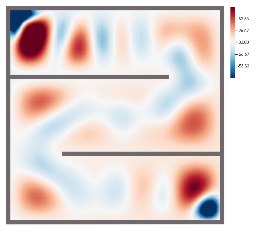
Figure 1: The potential that approximately minimizes the focusing metric for a two-dimensional gridworld maze. The agent begins in the top left of the grid and must navigate to the bottom right without hitting any of the exterior or interior walls.

We show the resulting potential $V$ that approximately minimizes $\mathcal{F}$ in Figure (1) and the state probability distribution over time for the optimally-trained agent in Figure (2). We see that the probability density focuses to a narrow target distribution at the final time as desired. In addition, the probablity density at all times navigates the barriers effectively to ensure zero probability of early termination of the agent maze navigation episode.

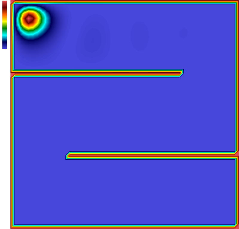
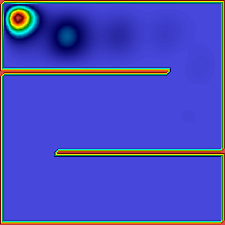
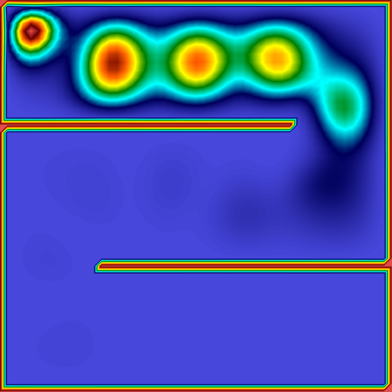
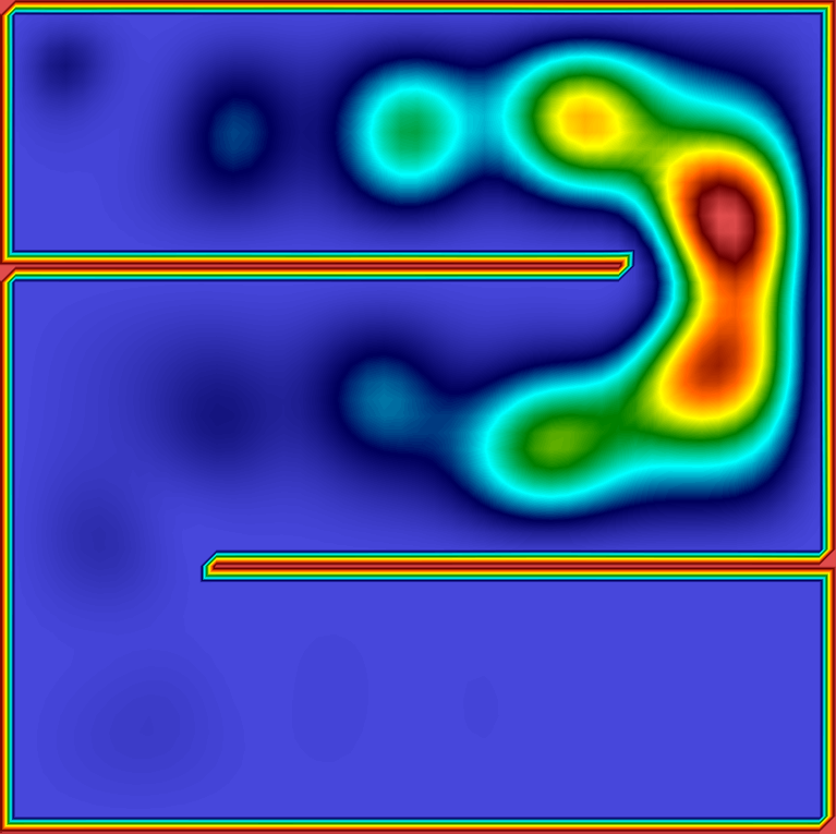
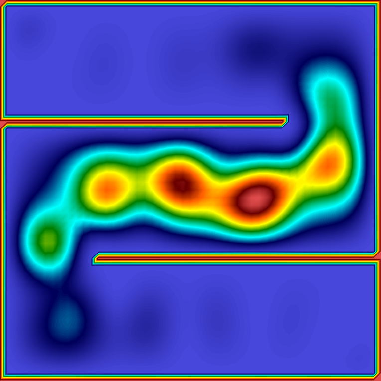
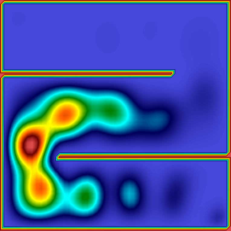
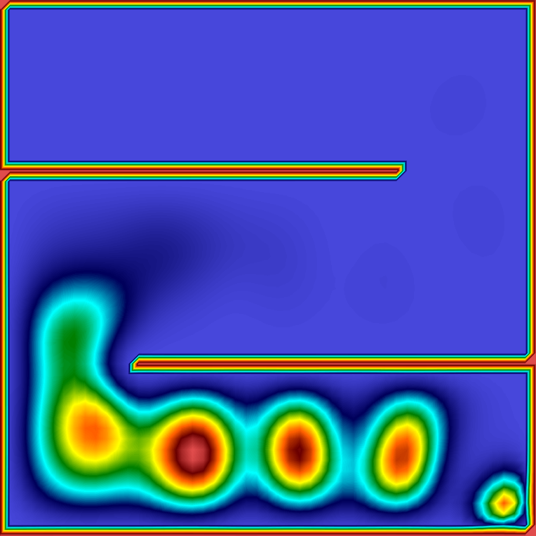
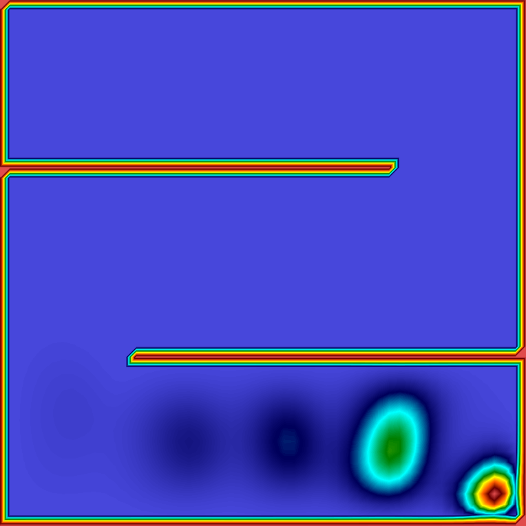
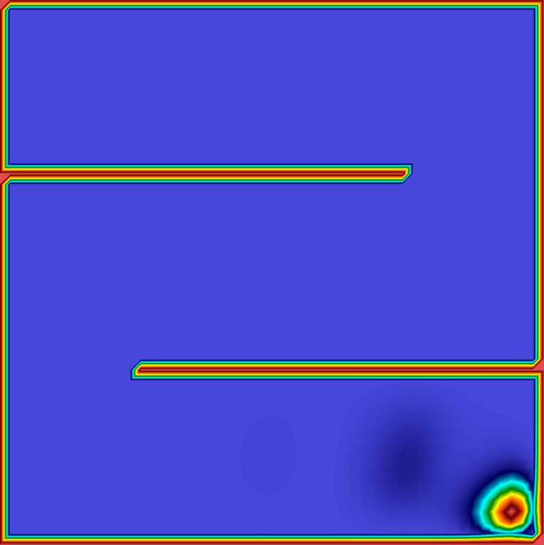
Figure 2: The agent state probability density as a function of time for the optimally controlled solution to navigating a gridworld maze. Time evolves in each panel from top left to bottom right.

Conclusions

We have shown that we can solve stochastic optimal control problems through computation of a potential function with an inverse scattering method. We assume we are given knowledge about the environment at the current time step and an asserted final time goal that the probability distribution of the agent state is ‘focused’ on specified state space locations. The control problem is then solved by computing the potential for all states and times that serves to drive an agent towards the goal. The potential is computed by matching the wavefunction solution of the Schrödinger equation to a desired target, which is a computation that can be executed in parallel across states and times.

The agent in this formulation is viewed as a dynamical system that follows ‘forces’ equal to the gradients of the potential function. Equivalently, the HJB optimal cost-to-go for the agent can be obtained from the phase of the wavefunction. While not demonstrated here, the approach admits a trivial generalization to multi-agent systems, where each agent learns its own potential.

Single-sided focusing minimizes the path length (in phase units) to reach a desired end state. Various paths considered in the variational context define a surface embedded in state space, whose area is the loss of information obtained by the agent relative to the optimal path [27]. For small deviations from the optimal path, the state cost function is determined by the probability distribution of the agent state, giving a localized description of the entire control solution that may be easily parallelized in future computational applications and can be contrasted with non-local Euclidean path integral methods [19] or episode-based training in RL [8].

The focusing action in Equation (14) is only one possible choice for determining the potential. Indeed, other actions are known to produce Euler-Lagrange equations that describe integrable systems, such as the Korteweg-de Vries (KdV) equation [48]. The optimal cost functions for control problems might then be derived as solutions to a broader class of integrable models. In the most general case of a time-dependent potential, the Schrödinger equation can be interpreted as one of the Lax operators [49] for a completely integrable dynamical model for the potential. This is another way that integrability can appear as a defining feature for solutions of stochastic optimal control problems.