Combined numerical methods for solving time-varying semilinear differential-algebraic equations with the use of spectral projectors and recalculation

Abstract

Two combined numerical methods for solving time-varying semilinear differential-algebraic equations (DAEs) are obtained. The convergence and correctness of the methods are proved. When constructing the methods, time-varying spectral projectors which can be found numerically are used. This enables to numerically solve the DAE in the original form without additional analytical transformations. To improve the accuracy of the second method, recalculation is used. The developed methods are applicable to the DAEs with the continuous nonlinear part which may not be differentiable in time, and the restrictions of the type of the global Lipschitz condition are not used in the presented theorems on the DAE global solvability and the convergence of the methods. This extends the scope of methods. The fulfillment of the conditions of the global solvability theorem ensures the existence of a unique exact solution on any given time interval, which enables to seek an approximate solution also on any time interval. Numerical examples illustrating the capabilities of the methods and their effectiveness in various situations are provided. To demonstrate this, mathematical models of the dynamics of electrical circuits are considered. It is shown that the results of the theoretical and numerical analyses of these models are consistent.

1 Introduction

Consider implicit differential equations

$$\frac{d}{dt}[A(t)x(t)]+B(t)x(t)=f(t,x(t))$$ (1)

$$A(t)\frac{d}{dt}x(t)+B(t)x(t)=f(t,x(t)),$$ (2)

and the initial condition

$$x(t_{0})=x_{0},$$ (3)

where $t\in[t_{+},\infty)$, $t_{0}\geq t_{+}\geq 0$, $f\in C([t_{+},\infty)\times{\mathbb{R}}^{n},{\mathbb{R}}^{n})$ and $A,\,B\in C([t_{+},\infty),\mathrm{L}({\mathbb{R}}^{n}))$  ($\mathrm{L}(X,Y)$ denotes the space of continuous linear operators acting from the vector space $X$ to the vector space $Y$;  $\mathrm{L}(X,X)=\mathrm{L}(X)$). The operators $A(t)$ and $B(t)$ can be degenerate (noninvertible). Equations of the type (1) and (2) with a degenerate (for some $t$) operator $A(t)$ are called degenerate differential equations or differential-algebraic equations (DAEs). In the DAE terminology, equations of the form (1), (2) are commonly referred to as semilinear. Since the operators $A(t)$, $B(t)$ are time-varying, the equations (1), (2) are called time-varying semilinear DAEs or time-varying degenerate differential equations (DEs). In what follows, for the sake of generality, the equations (1), (2), where $A(t)$  ($A\colon[t_{+},\infty)\to\mathrm{L}({\mathbb{R}}^{n})$) is an arbitrary (not necessarily degenerate) operator, will be called time-varying semilinear differential-algebraic equations.

The presence of a degenerate operator at the derivative in a DAE means the presence of algebraic constraints, namely, the graphs of the solutions must lie in the manifold generated by the “algebraic part” of the DAE and the initial points $(t_{0},x_{0})$ must also belong to this manifold (see Remark 1).

DAEs or degenerate DEs are also called descriptor equations (or descriptor systems), algebraic-differential systems, operator-differential equations and differential equations (or dynamical systems) on manifolds. These equations are used to describe mathematical models in control theory, radioelectronics, cybernetics, mechanics, economics, ecology, chemical kinetics and gas industry (see, e.g., BGHHSTisch ; Brenan-C-P ; BKT ; Fox-Jen-Zom ; HairerLR ; Kunkel_Mehrmann ; Lamour-Marz-Tisch ; Riaza ; Vlasenko1 and references therein). It is known that the dynamics of electrical circuits is modeled using DAEs which, in general, cannot be reduced to explicit ordinary differential equations (ODEs). In Sections 3.1 and 3.2 we will consider two mathematical models in the form of time-varying semilinear DAEs (1), which describes transient processes in electrical circuits.

A function $x\in C([t_{0},t_{1}),{\mathbb{R}}^{n})$  ($[t_{0},t_{1})\subseteq[t_{+},\infty)$) is said to be a solution of the equation (1) on $[t_{0},t_{1})$ if the function $A(t)x(t)$ is continuously differentiable on $[t_{0},t_{1})$ and $x(t)$ satisfies (1) on $[t_{0},t_{1})$. A function $x\in C^{1}([t_{0},t_{1}),{\mathbb{R}}^{n})$ is called a solution of the equation (2) on $[t_{0},t_{1})$ if $x(t)$ satisfies this equation on $[t_{0},t_{1})$. If the solution $x(t)$ of the equation (1) (the equation (2)) satisfies the initial condition (3), then it is called a solution of the initial value problem (IVP) or the Cauchy problem (1), (3)  (a solution of the IVP (2), (3)).

It is assumed that the operator pencil $\lambda A(t)+B(t)$ ($\lambda$ is a complex parameter) associated with the linear (left) part of the DAE (1) or (2) is a regular pencil of index not higher than 1 (index 0 or 1). This means that for each $t\geq t_{+}$ the pencil is regular, i.e., the set of its regular points is not empty (for the regular points $\lambda$ there exists the resolvent of pencil $(\lambda A(t)+B(t))^{-1}$), and there exist functions $C_{1},\,C_{2}\colon[t_{+},\infty)\to(0,\infty)$ such that for each $t\in[t_{+},\infty)$ the pencil resolvent

$$R(\lambda,t):=(\lambda A(t)+B(t))^{-1}$$

satisfies the condition (cf. Rut-Vlas2001 ; Vlasenko1 )

$$\|R(\lambda,t)\|\leq C_{1}(t),\quad|\lambda|\geq C_{2}(t)$$ (4)

(hence, for any fixed $t$ the resolvent is bounded in a neighborhood of infinity). The condition (4) means that either the point $\mu=0$ is a simple pole of the resolvent $(A(t)+\mu B(t))^{-1}$ of the pencil $A(t)+\mu B(t)$ (this is equivalent to the fact that $\lambda=\infty$ is a removable singularity of the resolvent $R(\lambda,t)$), or $\mu=0$ is a regular point of the pencil ${A(t)+\mu B(t)}$ (i.e., the operator $A(t)$ is nondegenerate). If $\mu=0$ is a regular point of the pencil $A(t)+\mu B(t)$ for each $t$, then $\lambda A(t)+B(t)$ is a regular pencil of index 0.  If $A(t)$ is degenerate for all $t$ and the condition (4) is satisfied (i.e., $\mu=0$ is a simple pole of the resolvent $(A(t)+\mu B(t))^{-1}$ for each $t$), then $\lambda A(t)+B(t)$ is a regular pencil of index 1. In the general case, the definition for the index of a regular pencil is given below.

In (Vlasenko1, , Section 6.2), for the regular pencil $\lambda A+B$ of time-invariant square matrices $A$ and $B$, the maximum length of the chain of root vectors of the pencil $A+\mu B$ at the point $\mu=0$ is referred to as the index of the pencil $\lambda A+B$. This definition can be naturally associated with the following generalization (cf. (Vlasenko1, , Section 3.3.1)) of the condition (4): Assume that the pencil $\lambda A(t)+B(t)$ is regular (for each $t\geq t_{+}$) and there exist functions $C_{1},\,C_{2}\colon[t_{+},\infty)\to(0,\infty)$ such that for each $t\in[t_{+},\infty)$,

$$\|R(\lambda,t)\|\leq C_{1}(t)|\lambda|^{\nu-1},\quad|\lambda|\geq C_{2}(t)\qquad(\nu\in{\mathbb{N}}),$$ (5)

then $\lambda A(t)+B(t)$ is called a regular pencil of index not higher than $\nu$. It follows from (5) that $\|(A(t)+\mu B(t))^{-1}\|\leq\dfrac{C_{1}(t)}{|\mu|^{\nu}}$,  $|\mu|\leq\dfrac{1}{C_{2}(t)}$. According to Vlasenko1 , we define the index of a regular pencil $\lambda A(t)+B(t)$ in the following way.

Let $A,\,B\colon\mathcal{T}\to\mathrm{L}(X,Y)$ (or $A(t)$, $B(t)$ are matrices corresponding to the linear operators $A(t),\,B(t)\in\mathrm{L}(X,Y)$ with respect to some bases in spaces $X$, $Y$, which depend on the parameter $t\in\mathcal{T}$), where $X=Y={\mathbb{R}}^{n}$ or $={\mathbb{C}}^{n}$ and $\mathcal{T}\subseteq{\mathbb{R}}$ is some interval, and the operator (or matrix) pencil $\lambda A(t)+B(t)$, where $\lambda$ is a complex parameter, is regular for each $t\in\mathcal{T}$. For a fixed $t\in\mathcal{T}$, if the point $\mu=0$ is a pole of the resolvent $(A(t)+\mu B(t))^{-1}$, then the order $\nu$ ($\nu\in{\mathbb{N}}$) of the pole is called the index of the regular pencil $\lambda A(t)+B(t)$, and in the case when $\mu=0$ is a regular point of the pencil $A(t)+\mu B(t)$, the index of the regular pencil $\lambda A(t)+B(t)$ is $\nu=0$. If the pencil $\lambda A(t)+B(t)$ has index $\nu$ for each $t\in\mathcal{T}$, then we will say that $\lambda A(t)+B(t)$ is a regular pencil of index $\nu$ ($\nu\in{\mathbb{N}}\cup\{0\}$). The same definition of the index of the regular pencil $\lambda A(t)+B(t)$ holds in the more general case when $A(t)$ and $B(t)$ are bounded linear operators (depending on the parameter $t$) from a Banach space $X$ to a Banach space $Y$.

Various notions of an index of the matrix (operator) pencil, an index of the DAE and a relationship between them are discussed, e.g., in (Fil.MPhAG, , Remark 2.1) and Lamour-Marz-Tisch ; Riaza .

If $\lambda A(t)+B(t)$ is a regular pencil of index not higher than $\nu$, i.e., the condition (5) holds, then for each $t\in[t_{+},\infty)$ there exist the two pairs of mutually complementary projectors Rut-Vlas2001 ; Vlasenko1

$$\begin{split}P_{1}(t)=\frac{1}{2\pi\mathrm{i}}\,\oint\limits_{|\lambda|=C_{2}(t)}R(\lambda,t)A(t)\,d\lambda,\qquad&Q_{1}(t)=\frac{1}{2\pi\mathrm{i}}\,\oint\limits_{|\lambda|=C_{2}(t)}A(t)R(\lambda,t)\,d\lambda,\\ P_{2}(t)=I_{{\mathbb{R}}^{n}}-P_{1}(t),\qquad&Q_{2}(t)=I_{{\mathbb{R}}^{n}}-Q_{1}(t)\qquad\end{split}$$ (6)

($P_{i}(t)P_{j}(t)=\delta_{ij}P_{i}(t)$, $P_{1}(t)+P_{2}(t)=I_{{\mathbb{R}}^{n}}$,  $Q_{i}(t)Q_{j}(t)=\delta_{ij}Q_{i}(t)$, $Q_{1}(t)+Q_{2}(t)=I_{{\mathbb{R}}^{n}}$, where $I_{{\mathbb{R}}^{n}}$ is the identity operator in ${\mathbb{R}}^{n}$, $\delta_{ij}$ is the Kronecker delta) which generate the direct decompositions of the spaces

$${\mathbb{R}}^{n}=X_{1}(t)\dot{+}X_{2}(t),\quad X_{j}(t)=P_{j}(t){\mathbb{R}}^{n},\qquad{\mathbb{R}}^{n}=Y_{1}(t)\dot{+}Y_{2}(t),\quad Y_{j}(t)=Q_{j}(t){\mathbb{R}}^{n},\quad j=1,2,$$ (7)

such that the pairs of subspaces $X_{1}(t)$, $Y_{1}(t)$ and $X_{2}(t)$, $Y_{2}(t)$ are invariant with respect to $A(t)$, $B(t)$ (i.e., $A(t),\,B(t)\colon X_{j}(t)\to Y_{j}(t)$); the restricted operators ${A_{j}(t)=\left.A(t)\right|_{X_{j}(t)}\colon X_{j}(t)\to Y_{j}(t)}$, $B_{j}(t)=\left.B(t)\right|_{X_{j}(t)}\colon X_{j}(t)\to Y_{j}(t)$, $j=1,2$, are such that the inverse operators $A_{1}^{-1}(t)$ and $B_{2}^{-1}(t)$ exist (if $X_{1}(t)\not=\{0\}$ and $X_{2}(t)\not=\{0\}$, respectively). If the regular pencil has index not higher than 1, i.e., satisfies (4), then ${A_{2}(t)=0}$ and the subspaces $X_{j}(t)$, $Y_{j}(t)$ are such that ${Y_{1}(t)=\mathcal{R}(A(t))}$ ($\mathcal{R}(A(t))$ is the range of $A(t)$), $X_{2}(t)=\mathop{\mathrm{Ker}}A(t)$, $Y_{2}(t)=B(t)X_{2}(t)$ and $X_{1}(t)=R(\lambda,t)Y_{1}(t)$, $|\lambda|\geq C_{2}(t)$. The spectral projectors (6) are real (because $A(t)$ and $B(t)$ are real) and $A(t)P_{1}(t)=Q_{1}(t)A(t)=A(t)$,  $A(t)P_{2}(t)=Q_{2}(t)A(t)=0$,  $B(t)P_{j}(t)=Q_{j}(t)B(t)$, $j=1,2$.

Using the spectral projectors, for each $t\in[t_{+},\infty)$ we obtain the auxiliary operator Rut-Vlas2001 ; Vlasenko1

$$G(t)=A(t)+B(t)P_{2}(t)=A(t)+Q_{2}(t)B(t)\in\mathrm{L}({\mathbb{R}}^{n})$$ (8)

such that $G(t)X_{j}(t)=Y_{j}(t)$, $j=1,2$; it has the inverse $G^{-1}(t)=A_{1}^{-1}(t)Q_{1}(t)+B_{2}^{-1}(t)Q_{2}(t)\in\mathrm{L}({\mathbb{R}}^{n})$ such that $G^{-1}(t)A(t)P_{1}(t)=G^{-1}(t)A(t)=P_{1}(t)$ and $G^{-1}(t)B(t)P_{2}(t)=P_{2}(t)$.

The projectors $P_{i}(t)$, $Q_{i}(t)$, $i=1,2$, and the operators $G(t)$, $G^{-1}(t)$ as operator functions have the same degree of smoothness as the operator functions $A(t)$, $B(t)$ and the function $C_{2}(t)$ from (4) (Vlasenko1, , Section 3.3).

In what follows, we suppose that $A,\,B\in C^{1}([t_{+},\infty),\mathrm{L}({\mathbb{R}}^{n}))$ and $C_{2}\in C^{1}([t_{+},\infty),(0,\infty))$, then $P_{i},\,Q_{i}\in C^{1}([t_{+},\infty),\mathrm{L}({\mathbb{R}}^{n}))$, $i=1,2$, and $G,\,G^{-1}\in C^{1}([t_{+},\infty),\mathrm{L}({\mathbb{R}}^{n}))$. Since the projectors $P_{i}(t)$, $Q_{i}(t)$ are continuous (moreover, they are continuously differentiable) as operator functions for $t\in[t_{+},\infty)$, the dimensions of the subspaces $X_{i}(t)=P_{i}(t){\mathbb{R}}^{n}$ and $Y_{i}(t)=Q_{i}(t){\mathbb{R}}^{n}$ ($i=1,2$) are constant (cf. (Kato-eng, , p. 34)), and we denote ${\dim X_{2}(t)=\dim Y_{2}(t)=d}$ ($d=const\geq 0$) and, accordingly, $\dim X_{1}(t)=\dim Y_{1}(t)=n-d$, $t\in[t_{+},\infty)$. This means that the pencil $\lambda A(t)+B(t)$ has either index 0 for each $t$ or index 1 for each $t$  ($t\in[t_{+},\infty)$).

For each $t$, any $x\in{\mathbb{R}}^{n}$ is uniquely representable with respect to the decomposition (7) in the form

$$x=P_{1}(t)x+P_{2}(t)x=x_{p_{1}}(t)+x_{p_{2}}(t),\quad x_{p_{i}}(t)=P_{i}(t)x\in X_{i}(t).$$ (9)

By using projectors $P_{i}(t)$, $Q_{i}(t)$ and operator $G^{-1}(t)$ the DAE (1) is reduced to the equivalent system of the explicit ODE (10) (with respect to $P_{1}(t)x(t)$) and the algebraic equation (AE) (11):

$$[P_{1}(t)x(t)]^{\prime}=\big{[}P^{\prime}_{1}(t)-G^{-1}(t)\,Q_{1}(t)\,[A^{\prime}(t)+B(t)]\,\big{]}P_{1}(t)x(t)+G^{-1}(t)\,Q_{1}(t)f(t,x(t)),$$ (10)

$$G^{-1}(t)\,Q_{2}(t)\big{[}f(t,x(t))-A^{\prime}(t)P_{1}(t)x(t)\big{]}-P_{2}(t)x(t)=0.$$ (11)

Using the representation (9)  ($x_{p_{i}}(t)=P_{i}(t)x(t)$), we write the system (10), (11) in the form

$$x_{p_{1}}^{\prime}(t)=\big{[}P^{\prime}_{1}(t)-G^{-1}(t)\,Q_{1}(t)\,[A^{\prime}(t)+B(t)]\,\big{]}x_{p_{1}}(t)+G^{-1}(t)\,Q_{1}(t)f\big{(}t,x_{p_{1}}(t)+x_{p_{2}}(t)\big{)},$$ (12)

$$G^{-1}(t)\,Q_{2}(t)\big{[}f\big{(}t,x_{p_{1}}(t)+x_{p_{2}}(t)\big{)}-A^{\prime}(t)x_{p_{1}}(t)\big{]}-x_{p_{2}}(t)=0.$$ (13)

The system (12), (13) or (10), (11) is a nonautonomous (time-varying) semi-explicit DAE. Generally, systems of the form $\dot{y}=f(t,y,z)$, $0=g(t,y,z)$ are referred to as nonautonomous (time-varying) semi-explicit DAEs.

Similarly, the DAE (2) is reduced to the equivalent system (the semi-explicit form)

$$[P_{1}(t)x(t)]^{\prime}=G^{-1}(t)[-B(t)P_{1}(t)x(t)+Q_{1}(t)f(t,x(t))]+P^{\prime}_{1}(t)x(t),$$

$$G^{-1}(t)Q_{2}(t)f(t,x(t))-P_{2}(t)x(t)=0.$$

or (taking into account the representation (9))

$$x_{p_{1}}^{\prime}(t)=G^{-1}(t)[-B(t)x_{p_{1}}(t)+Q_{1}(t)f(t,x_{p_{1}}(t)+x_{p_{2}}(t))]+P^{\prime}_{1}(t)(x_{p_{1}}(t)+x_{p_{2}}(t)),$$ (14)

$$G^{-1}(t)Q_{2}(t)f(t,x_{p_{1}}(t)+x_{p_{2}}(t))-x_{p_{2}}(t)=0.$$

Numerical methods for solving various types of DAEs are presented in Hairer-W ; HairerLR ; Lamour-Marz-Tisch ; Kunkel_Mehrmann ; Linh-Mehrmann ; Brenan-C-P ; Ascher-Petz ; Knorrenschild ; HankeMarTiWeinW ; Fil.CombMeth (also, see references therein). Generally, there are already a lot of works on this topic. The main idea of many works is the reduction of a DAE to an ODE or the replacement of a DAE by a stiff ODE for the further application of the methods for solving ODEs, or the use of these methods directly for solving DAEs. For example, to solve the autonomous semi-explicit DAE $y^{\prime}=f(y,z)$, $0=g(y,z)$ of index 1 (it has index 1 for all $y$, $z$ such that $[\partial g(y,z)/\partial z]^{-1}$ exists and is bounded), the $\varepsilon$-embedding method is applied in Hairer-W ; HairerLR . For the nonautonomous semi-explicit DAE $y^{\prime}=f(t,y,z)$, $0=g(t,y,z)$ of index 1, the similar $\varepsilon$-embedding method in which the Runge-Kutta (RK) method is applied to the corresponding stiff system $y^{\prime}=f(t,y,z,\varepsilon)$, $\varepsilon z^{\prime}=g(t,y,z)$ ($\varepsilon\to 0$) and then $\varepsilon=0$ is set in the resulting formulas is presented in Knorrenschild ; Kunkel_Mehrmann ; Ascher-Petz ; Brenan-C-P . A solution of the stiff system of ODEs $y^{\prime}=f(t,y,z,\varepsilon)$, $\varepsilon z^{\prime}=g(t,y,z,\varepsilon)$ ($\varepsilon>0$) in general does not approach the solution of the reduced DAE (obtained by setting $\varepsilon=0$)  $y^{\prime}=f(t,y,z,0)$, $0=g(t,y,z,0)$, however, under certain conditions it is possible to obtain a stiff ODE system whose solutions approximate solutions of the reduced DAE Knorrenschild ; Brenan-C-P . The backward differentiation formulas (BDF) method, RK method and general linear multi-step methods were presented for semi-explicit DAEs and regular nonlinear DAEs of index 1 in Kunkel_Mehrmann ; Lamour-Marz-Tisch ; Ascher-Petz ; Brenan-C-P and also for regular time-invariant quasilinear DAEs in Hairer-W . In Kunkel_Mehrmann ; Linh-Mehrmann , the collocation RK method, the BDF method and a half-explicit method were given for regular strangeness-free DAEs. The aforementioned methods are also applied for DAEs of index higher than 1. The application of the RK methods to semi-explicit DAEs of index 2 or 3 are described, e.g., in Ascher-Petz ; Brenan-C-P ; Hairer-W ; HairerLR , SatoMdA . A least-squares collocation method was constructed for linear higher-index DAEs in HankeMarTiWeinW . Also, there exist numerical methods for the reduction of the index of DAEs (see, e.g., Ascher-Petz ; Kunkel_Mehrmann ; Lamour-Marz-Tisch ; Hairer-W ).

In the present paper, we obtain numerical methods for the time-varying semilinear DAEs, using, in particular, the time-varying spectral projectors (6). Earlier (see Fil.CombMeth ), numerical methods for the time-invariant semilinear DAEs were developed using, accordingly, time-invariant spectral projectors. Also, we use the scheme with recalculation (the “predictor-corrector” scheme) which was not used in Fil.CombMeth .

The paper has the following structure. In Section 1, we consider the constraints on the operator coefficients (more precisely, on the characteristic operator pencils) of the DAEs (1) and (2), give the necessary definitions and describe the method for reducing the time-varying semilinear DAE to an equivalent semi-explicit form by using the spectral projectors. In Section 2, the two combined methods for solving the time-varying semilinear DAEs are obtained, and the theorems giving conditions for their convergence and correctness and indicating the orders of accuracy of the methods with respect to the step size (the global errors) are proved. The important remarks on the convergence of the methods, when weakening the smoothness requirements for the nonlinear functions in the DAEs, are given in Section 2. Note that in Sections 2, 3.1, 3.2 when proving the theorems, as well as when analyzing mathematical models, we use the results presented in Appendix. Appendix provides theorems and propositions (proved in prior papers), which give conditions for the existence, uniqueness and boundedness of exact global solutions, as well as certain definitions and the remarks on the solution properties and the theorem applications. In Sections 3.1, 3.2 the theoretical and numerical analyses of mathematical models of the dynamics of electric circuits are carried out, which, on the one hand, demonstrates the application of the obtained theorems and methods to real physical problems, and on the other hand, shows that the theoretical and numerical results are consistent. In Section 3.3, the comparative analysis of the methods is carried out.

In the paper, a function, for example $f$, is often denoted by the same symbol $f(x)$ as its value at the point $x$ in order to explicitly indicate its argument (or arguments), but it will be clear from the context what exactly is meant. Notice that when the formula breaks at the multiplication sign, we denote it by $\times$.

2 Combined numerical methods: the construction, convergence and orders of accuracy

One of the advantages of the numerical methods proposed in this paper is the possibility to numerically find the spectral projectors $P_{i}(t)$, $Q_{i}(t)$ (and, as a consequence, the operator $G(t)$), which enables to numerically solve the DAE in the original form (1) or (2), i.e., additional analytical transformations are not required for the application of the numerical methods. To calculate the spectral projectors, residues can be used (see (15) below). Recall that, by assumption, the pencil $\lambda A(t)+B(t)$ is either a regular pencil of index 1 or a regular pencil of index 0. The definition of the index of a regular pencil is given in Section 1.

Now, suppose that $\lambda A(t)+B(t)$ is a regular pencil of index $\nu$  (${\nu\in{\mathbb{N}}\cup\{0\}}$). It follows from (6) that ${P_{1}(t)=\displaystyle\dfrac{1}{2\pi\mathrm{i}}\oint\limits_{|\mu|=1/C_{2}(t)}\dfrac{(A(t)+\mu B(t))^{-1}A(t)}{\mu}d\mu}$ and ${Q_{1}(t)=\displaystyle\dfrac{1}{2\pi\mathrm{i}}\oint\limits_{|\mu|=1/C_{2}(t)}\dfrac{A(t)(A(t)+\mu B(t))^{-1}}{\mu}d\mu}$. Thus, for each $t\in[t_{+},\infty)$ the projectors (6) can be calculated by using residues:

$$\begin{split}P_{1}(t)=\mathop{\mathrm{Res}}\limits_{\mu=0}\left(\dfrac{(A(t)+\mu B(t))^{-1}A(t)}{\mu}\right),\qquad&Q_{1}(t)=\mathop{\mathrm{Res}}\limits_{\mu=0}\left(\dfrac{A(t)(A(t)+\mu B(t))^{-1}}{\mu}\right),\\ P_{2}(t)=I_{{\mathbb{R}}^{n}}-P_{1}(t),\qquad&Q_{2}(t)=I_{{\mathbb{R}}^{n}}-Q_{1}(t).\end{split}$$ (15)

Denote ${R_{p}(\mu,t):=\dfrac{(A(t)+\mu B(t))^{-1}A(t)}{\mu}}$ and ${R_{q}(\mu,t):=\dfrac{A(t)(A(t)+\mu B(t))^{-1}}{\mu}}$, then ${P_{1}(t)=\mathop{\mathrm{Res}}\limits_{\mu=0}R_{p}(\mu,t)}$ and ${Q_{1}(t)=\mathop{\mathrm{Res}}\limits_{\mu=0}R_{q}(\mu,t)}$, where $t$ is a parameter. It is clear that the function $(R_{p})_{ij}(\mu,t)$ ($i,j=1,...,n$), i.e., $(i,j)$-entry of the matrix $R_{p}(\mu,t)$, is a rational function in $\mu$, and if $\mu=0$ is its pole of order $k$, then $(R_{p})_{ij}(\mu,t)=\varphi(\mu,t)\mu^{-k}$, where $\varphi(\mu,t)$ is a polynomial in $\mu$ such that $\varphi(0,t)\neq 0$ (similarly for $(R_{q})_{ij}(\mu,t)$). The main steps of the algorithm used for the calculation of the projectors (15) are as follows:

1. First option. For $i,j=1,...,n$:   1.1. determine the order $k$ of a pole of the function $(R_{p})_{ij}(\mu,t)$ at the point $\mu=0$; to do this, we convert $(R_{p})_{ij}(\mu,t)$ to a rational form (with respect to $\mu$) and determine the order $k$ of the zero of the denominator at the point $\mu=0$, at that, if the denominator does not have a zero at $\mu=0$, then the order $k=0$;   1.2. if the order $k\geq 1$, then ${(P_{1})_{ij}(t)=\mathop{\mathrm{Res}}\limits_{\mu=0}(R_{p})_{ij}(\mu,t)=\dfrac{1}{(k-1)!}\dfrac{d^{k-1}}{d\mu^{k-1}}\big{[}(R_{p})_{ij}(\mu,t)\,\mu^{k}\big{]}\bigg{|}_{\mu=0}}$, and if the order $k=0$, then $(P_{1})_{ij}(t)=0$. Finally, $P_{1}(t)=\big{(}(P_{1})_{ij}(t)\big{)}_{1\leq i,j\leq n}$.

   Second option (calculation of the entire projector at once).   1.1. determine the order $\nu$ of a pole of $R_{p}(\mu,t)$ at the point $\mu=0$ (to do this, we can determine the order $k_{ij}=k$ of a pole of $(R_{p})_{ij}(\mu,t)$ at $\mu=0$ as described in 1.1 above, and set $\nu=\max\limits_{i,j=1,...,n}\{k_{ij}\}$);   1.2. if the order $\nu\geq 1$, then ${P_{1}(t)=\mathop{\mathrm{Res}}\limits_{\mu=0}R_{p}(\mu,t)=\dfrac{1}{(\nu-1)!}\dfrac{d^{\nu-1}}{d\mu^{\nu-1}}\big{[}R_{p}(\mu,t)\,\mu^{\nu}\big{]}\bigg{|}_{\mu=0}}$, and if $\nu=0$, then $P_{1}(t)=0$.

2. Perform the same as in Step 1, replacing $R_{p}(\mu,t)=\big{(}(R_{p})_{ij}(\mu,t)\big{)}_{1\leq i,j\leq n}$ with $R_{q}(\mu,t)=\big{(}(R_{q})_{ij}(\mu,t)\big{)}_{1\leq i,j\leq n}$ and, accordingly, $P_{1}(t)$ with $Q_{1}(t)=\big{(}(Q_{1})_{ij}(t)\big{)}_{1\leq i,j\leq n}$.

3. Having calculated $P_{1}(t)$ and $Q_{1}(t)$, find $P_{2}(t)=I_{{\mathbb{R}}^{n}}-P_{1}(t)$ and $Q_{2}(t)=I_{{\mathbb{R}}^{n}}-Q_{1}(t)$.

In the case when the index of the pencil $\lambda A(t)+B(t)$ is 0, we have ${P_{1}(t)\equiv I_{{\mathbb{R}}^{n}}}$, ${P_{2}(t)\equiv 0}$, and ${Q_{1}(t)\equiv I_{{\mathbb{R}}^{n}}}$, ${Q_{2}(t)\equiv 0}$. In this case, the operator $A(t)$ is nondegenerate (invertible) for each $t\in[t_{+},\infty)$ and the DAEs (1) and (2) can be reduced to ODEs. Obviously, in the case when $A(t)\equiv 0$ and $B(t)$ is nondegenerate for each $t$, which corresponds to the particular case of the pencil $\lambda A(t)+B(t)$ of index 1, we have $P_{1}(t)\equiv 0$, $P_{2}(t)\equiv I_{{\mathbb{R}}^{n}}$, and $Q_{1}(t)\equiv 0$, $Q_{2}(t)\equiv I_{{\mathbb{R}}^{n}}$, and, in this case, (1), (2) are purely algebraic equations (do not contain the derivative).

After computing the projectors, the auxiliary operator $G(t)$ is calculated by (8).

For the special cases when $A(t)$ is nondegenerate or is zero (for all $t$), the results obtained herein remain valid, but since the purpose of the paper was to construct numerical methods for the DAEs, we carry out further proofs for the case when $A(t)$ is degenerate but not identically zero and $\lambda A(t)+B(t)$ is a regular pencil of index 1, without comments on the form of the conditions for the special cases.

The theorems on the of global solvability and on the Lagrange stability, presented in Appendix, ensure the existence of a unique exact solution of the IVP for the DAE on the interval $[t_{0},\infty)$ (the Lagrange stability additionally guarantees the boundedness of solutions). This enables to compute approximate solutions on any given time interval $[t_{0},T]$ when performing the conditions of the theorems or remarks on the convergence of the methods, presented below. This was important to note, since in many works when proving the convergence of a method it is assumed in advance that there is a unique exact solution on the interval where the computation will be carried out, while the calculation of the allowable length of this interval is a separate problem. In addition, one often uses theorems allowing to prove the existence and uniqueness of an exact solution only on a sufficiently small (local) time interval, but in this case the numerical method can be correctly applied only on this small interval.

Note that the developed methods are applicable to DAEs of the type (1), (2) with the continuous nonlinear part which may not be differentiable in $t$ (see Remarks 2, 3). This is important for applications, since such equations arise in various practical problems, for example, the functions of currents and voltages in electric circuits may not be differentiable (or be piecewise differentiable) or may be approximated by nondifferentiable functions. As examples, nonsinusoidal currents and voltages of the “sawtooth”, “triangular” and “rectangular” shapes Erickson-Maks ; Borisov-Lip-Zor can be considered, but more complex shapes are also occurred. In Sections 3.1.2 and 3.2.2 , the examples of numerical solutions for electrical circuits with nondifferentiable (on a given time interval) functions of voltages, namely, the voltages of the triangular and sawtooth shapes, are presented (Fig. 4 and 9). Also note that the restrictions of the type of the global Lipschitz condition, including the global condition of the contractivity (the Lipschitz condition with a constant less than 1), are not used in the theorems on the DAE global solvability and on the convergence of the methods, and it is not required that the pencil $\lambda A(t)+B(t)-\frac{\partial f}{\partial x}(t,x)$ be a regular pencil of index 1 (i.e., that the DAEs under consideration be regular DAEs of tractability index 1). The global Lipschitz condition is not fulfilled for mathematical models of electrical circuits with certain nonlinear parameters (e.g., in the form of power functions mentioned in Section 3.1, 3.2). In general, various types of DEs with non-Lipschitz or non-globally Lipschitz functions (see, e.g., IzgiCetin and references therein) arise in applications.

Remark 1

(Fil.DE-1, , Remark 1.2) Introduce the manifolds

$$L_{t_{+}}=\{(t,x)\in[t_{+},\infty)\times{\mathbb{R}}^{n}\mid Q_{2}(t)[A^{\prime}(t)P_{1}(t)x+B(t)x-f(t,x)]=0\},$$ (16)

$$\widehat{L}_{t_{+}}=\{(t,x)\in[t_{+},\infty)\times{\mathbb{R}}^{n}\mid Q_{2}(t)[B(t)x-f(t,x)]=0\}$$ (17)

(in (16), (17) the number $t_{+}$ is a parameter). The consistency condition $(t_{0},x_{0})\in L_{t_{+}}$ ($(t_{0},x_{0})\in\widehat{L}_{t_{+}}$) for the initial point $(t_{0},x_{0})$ is one of the necessary conditions for the existence of a solution of the IVP (1), (3)  (the IVP (2), (3)). An initial point $(t_{0},x_{0})$ satisfying this condition is called a consistent initial point (the corresponding initial values $t_{0}$, $x_{0}$ are called consistent initial values).

We will seek a solution $x(t)$ of the IVP (1), (3) on an interval $[t_{0},T]$. Introduce the uniform mesh $\omega_{h}=\{t_{i}=t_{0}+ih,\;i=0,...,N,\;t_{N}=T\}$ with the step $h=(T-t_{0})/N$ on $[t_{0},T]$. The values of an approximate solution at the points $t_{i}$ are denoted by $x_{i}$, $i=0,...,N$.

Initial value $x_{0}$ for the IVP (1), (3) and, accordingly, initial values $z_{0}=P_{1}(t_{0})x_{0}$, $u_{0}=P_{2}(t_{0})x_{0}$ are chosen so that the consistency condition $Q_{2}(t_{0})\big{[}A^{\prime}(t_{0})P_{1}(t_{0})x_{0}+B(t_{0})x_{0}-f(t_{0},x_{0})\big{]}=0$, i.e., $(t_{0},x_{0})\in L_{t_{+}}$, is fulfilled. The consistency condition $(t_{0},x_{0})\in L_{t_{+}}$ for the initial values $t_{0}$, $x_{0}$ ensures the best choice of the initial values for the developed methods (more precisely, for the methods applied to the “algebraic part” of the DAE).

Below, Theorems 3.1, 3.2 and other results which are presented in Appendix are used.

2.1 Method 1 (the simple combined method)

Theorem 2.1

Let the conditions of Theorem 3.1 or 3.2 be satisfied and, additionally, the operator ${\Phi_{t_{*},P_{1}(t_{*})z_{*},P_{2}(t_{*})u_{*}}=\Phi_{t_{*},P_{1}(t_{*})z_{*}}(P_{2}(t_{*})u_{*})\colon X_{2}(t_{*})\to Y_{2}(t_{*})}$, which is defined by (94) or (97) for each (fixed) $t_{*}$, each ${x^{*}_{p_{1}}(t_{*})=P_{1}(t_{*})z_{*}}$ and each ${x^{*}_{p_{2}}(t_{*})=P_{2}(t_{*})u_{*}}$,  be invertible for each point ${(t_{*},P_{1}(t_{*})z_{*}+P_{2}(t_{*})u_{*})\in[t_{0},T]\times{\mathbb{R}}^{n}}$. In addition, let $A,\,B\in C^{2}([t_{0},T],\mathrm{L}({\mathbb{R}}^{n}))$, $C_{2}\in C^{2}([t_{0},T],(0,\infty))$ (recall that the function $C_{2}(t)$ was introduced in (4)), $f\in C^{1}([t_{0},T]\times{\mathbb{R}}^{n},{\mathbb{R}}^{n})$ and an initial value $x_{0}$ be chosen so that the consistency condition $(t_{0},x_{0})\in L_{t_{+}}$ (i.e., ${Q_{2}(t_{0})\big{[}A^{\prime}(t_{0})P_{1}(t_{0})x_{0}+B(t_{0})x_{0}-f(t_{0},x_{0})\big{]}=0}$) be satisfied. Then the method

$$z_{0} =P_{1}(t_{0})x_{0},\quad u_{0}=P_{2}(t_{0})x_{0},$$ (18)

$$z_{i+1} =\Big{(}I_{{\mathbb{R}}^{n}}+h\big{[}P^{\prime}_{1}(t_{i})-G^{-1}(t_{i})Q_{1}(t_{i})[A^{\prime}(t_{i})+B(t_{i})]\big{]}P_{1}(t_{i})\Big{)}z_{i}+h\,G^{-1}(t_{i})Q_{1}(t_{i})f\big{(}t_{i},x_{i}\big{)},$$ (19)

$$\begin{split}u_{i+1}&=u_{i}-\!\bigg{[}I_{{\mathbb{R}}^{n}}-G^{-1}(t_{i+1})Q_{2}(t_{i+1})\dfrac{\partial f}{\partial x}\big{(}t_{i+1},P_{1}(t_{i+1})z_{i+1}+P_{2}(t_{i+1})u_{i}\big{)}\,P_{2}(t_{i+1})\bigg{]}^{-1}\!\bigg{[}u_{i}-{}\\ &-G^{-1}(t_{i+1})Q_{2}(t_{i+1})\Big{[}f\big{(}t_{i+1},P_{1}(t_{i+1})z_{i+1}+P_{2}(t_{i+1})u_{i}\big{)}-A^{\prime}(t_{i+1})P_{1}(t_{i+1})z_{i+1}\Big{]}\bigg{]},\end{split}$$ (20)

$$x_{i+1} =P_{1}(t_{i+1})z_{i+1}+P_{2}(t_{i+1})u_{i+1},\quad t_{i+1}\in\omega_{h},\quad i=0,...,N-1,$$ (21)

approximating the IVP (1), (3) on $[t_{0},T]$ converges and has the first order of accuracy: $\max\limits_{0\leq i\leq N}\|x(t_{i})-x_{i}\|=O(h)$, $h\to 0$ ($\max\limits_{0\leq i\leq N}\|z(t_{i})-z_{i}\|=O(h)$, $\max\limits_{0\leq i\leq N}\|u(t_{i})-u_{i}\|=O(h)$, $h\to 0$).

Proof

Take any initial point $(t_{0},x_{0})\in L_{t_{+}}$ (i.e., $Q_{2}(t_{0})\big{[}A^{\prime}(t_{0})P_{1}(t_{0})x_{0}+B(t_{0})x_{0}-f(t_{0},x_{0})\big{]}=0$). By virtue of the theorem conditions, taking into account Remark 5 (see Appendix), we obtain that for each initial point $(t_{0},x_{0})\in L_{t_{+}}$ there exists a unique global (exact) solution $x(t)$ of the IVP (1), (3) such that $z(t)=P_{1}(t)x(t)\in C^{2}([t_{0},T],{\mathbb{R}}^{n})$ and $u(t)=P_{2}(t)x(t)\in C^{1}([t_{0},T],{\mathbb{R}}^{n})$ ($z\in C^{1}([t_{0},\infty),{\mathbb{R}}^{n})$, $u\in C([t_{0},\infty),{\mathbb{R}}^{n})$ and $z(t)\in X_{1}(t)$, $u(t)\in X_{2}(t)$).

The DAE (1) is equivalent to the system (12), (13) which can be written in the form:

$$x_{p_{1}}^{\prime}(t)=\big{[}P^{\prime}_{1}(t)-G^{-1}(t)\,Q_{1}(t)\,[A^{\prime}(t)+B(t)]\,\big{]}x_{p_{1}}(t)+G^{-1}(t)\,Q_{1}(t)f\big{(}t,x_{p_{1}}(t)+x_{p_{2}}(t)\big{)},$$

$$x_{p_{2}}(t)=G^{-1}(t)\,Q_{2}(t)\big{[}f\big{(}t,x_{p_{1}}(t)+x_{p_{2}}(t)\big{)}-A^{\prime}(t)x_{p_{1}}(t)\big{]}.$$

Let us introduce mappings $\Pi,\,F\colon[t_{+},\infty)\times{\mathbb{R}}^{n}\times{\mathbb{R}}^{n}\to{\mathbb{R}}^{n}$ of the following form:

$$\Pi(t,z,u):=\big{[}P^{\prime}_{1}(t)-G^{-1}(t)\,Q_{1}(t)\,[A^{\prime}(t)+B(t)]\,\big{]}P_{1}(t)z+G^{-1}(t)\,Q_{1}(t)\,f(t,P_{1}(t)z+P_{2}(t)u),$$ (22)

$$F(t,z,u):=G^{-1}(t)\,Q_{2}(t)\big{[}f(t,P_{1}(t)z+P_{2}(t)u)-A^{\prime}(t)\,P_{1}(t)z\big{]}-u$$ (23)

(note that $Q_{2}(t)A^{\prime}(t)=Q_{2}(t)A^{\prime}(t)P_{1}(t)$). These mappings are continuous in $(t,z,u)$ and have continuous partial derivatives with respect to $z$, $u$ on $[t_{+},\infty)\times{\mathbb{R}}^{n}\times{\mathbb{R}}^{n}$ due to the conditions of Theorem 2.1, as well as Remarks 2 presented below, and, in addition, they have a continuous partial derivative with respect to $t$ on $[t_{+},\infty)\times{\mathbb{R}}^{n}\times{\mathbb{R}}^{n}$ due to the conditions of the theorem.

Consider the system

$$z^{\prime}(t)=\Pi(t,z(t),u(t)),$$ (24)

$$F(t,z(t),u(t))=0.$$ (25)

Lemma 1 ((Fil.DE-1, , Lemma 2.1))

If a function $x(t)$ is a solution of the DAE (1) on $[t_{0},t_{1})$ and satisfies the initial condition (3), then the functions $z(t)=P_{1}(t)x(t)$, $u(t)=P_{2}(t)x(t)$ are a solution of the system (24), (25) on $[t_{0},t_{1})$, satisfy the initial conditions $z(t_{0})=P_{1}(t_{0})x_{0}$, $u(t_{0})=P_{2}(t_{0})x_{0}$, and $z\in C^{1}([t_{0},t_{1}),{\mathbb{R}}^{n})$, $u\in C([t_{0},t_{1}),{\mathbb{R}}^{n})$.

Conversely, if functions $z\in C^{1}([t_{0},t_{1}),{\mathbb{R}}^{n})$, $u\in C([t_{0},t_{1}),{\mathbb{R}}^{n})$ are a solution of the system (24), (25) on $[t_{0},t_{1})$ and satisfy the initial conditions $z(t_{0})=P_{1}(t_{0})x_{0}$, $u(t_{0})=P_{2}(t_{0})x_{0}$, then $P_{1}(t)z(t)=z(t)$, $P_{2}(t)u(t)=u(t)$ and the function $x(t)=z(t)+u(t)$ is a solution of the DAE (1) on $[t_{0},t_{1})$ and satisfies the initial condition (3).

Denote

$$W(t,z,u):=G^{-1}(t)\,Q_{2}(t)\big{[}f(t,P_{1}(t)z+P_{2}(t)u)-A^{\prime}(t)P_{1}(t)z\big{]}$$ (26)

and write the system (24), (25) in the form

$$z^{\prime}(t)=\Pi(t,z(t),u(t)),$$ (27)

$$u(t)=W(t,z(t),u(t)).$$ (28)

Note that if $u(t)\in{\mathbb{R}}^{n}$ satisfies the relation (25) or the equivalent relation (28), then $u(t)\in X_{2}(t)$ (i.e., $u(t)=P_{2}(t)u(t)$).

Using the equality (28) where $t$ is replaced by $t+h$ and the Taylor expansion

$$W\big{(}t+h,z(t+h),u(t+h)\big{)}\!=W\big{(}t+h,z(t+h),u(t)\big{)}+\\ +\dfrac{\partial W}{\partial u}\big{(}t+h,z(t+h),u(t)\big{)}\big{[}u(t+h)-u(t)\big{]}+O(h),$$ (29)

where

$$\dfrac{\partial W}{\partial u}\big{(}t+h,z(t+h),u(t)\big{)}\!=G^{-1}(t+h)Q_{2}(t+h)\dfrac{\partial f}{\partial x}\big{(}t+h,P_{1}(t+h)z(t+h)+P_{2}(t+h)u(t)\big{)}\,P_{2}(t+h),$$ (30)

we obtain the relation

$$u(t+h)=\!\bigg{[}I_{{\mathbb{R}}^{n}}-\dfrac{\partial W}{\partial u}\big{(}t+h,z(t+h),u(t)\big{)}\bigg{]}^{-1}\bigg{[}W\big{(}t+h,z(t+h),u(t)\big{)}-\dfrac{\partial W}{\partial u}\big{(}t+h,z(t+h),u(t)\big{)}\,u(t)+\\ +O(h)\bigg{]}=\bigg{[}I_{{\mathbb{R}}^{n}}-G^{-1}(t+h)Q_{2}(t+h)\dfrac{\partial f}{\partial x}\big{(}t+h,P_{1}(t+h)z(t+h)+P_{2}(t+h)u(t)\big{)}\,P_{2}(t+h)\bigg{]}^{-1}\times\\ \times\bigg{[}G^{-1}(t+h)Q_{2}(t+h)\Big{(}f\big{(}t+h,P_{1}(t+h)z(t+h)+P_{2}(t+h)u(t)\big{)}-A^{\prime}(t+h)P_{1}(t+h)z(t+h)-\\ -\dfrac{\partial f}{\partial x}\big{(}t+h,P_{1}(t+h)z(t+h)+P_{2}(t+h)u(t)\big{)}\,P_{2}(t+h)u(t)\Big{)}+O(h)\bigg{]}.$$ (31)

The relation (31) can be rewritten as

$$u(t+h)\!=\!u(t)-\!\bigg{[}I_{{\mathbb{R}}^{n}}\!-G^{-1}(t+h)Q_{2}(t+h)\dfrac{\partial f}{\partial x}\big{(}t+h,P_{1}(t+h)z(t+h)+P_{2}(t+h)u(t)\big{)}P_{2}(t+h)\bigg{]}^{-1}\!\Big{[}u(t)-\\ -G^{-1}(t+h)Q_{2}(t+h)\Big{(}f\big{(}t+h,P_{1}(t+h)z(t+h)+P_{2}(t+h)u(t)\big{)}-A^{\prime}(t+h)P_{1}(t+h)z(t+h)\Big{)}\Big{]}+\\ +O(h).$$ (32)

As a result, for the algebraic equation (28) we obtain a method similar to the Newton method with respect to the component $u$ of the phase variable $x=z+u$. The existence of the inverse operator used in the relations above follows from the following statement: From the invertibility of the operator $\Phi_{t,P_{1}(t)z,P_{2}(t)u}$ (if in the theorem conditions it is assumed that the requirements of Theorem 3.1 are satisfied) and the basis invertibility of the operator function $\Phi_{t,P_{1}(t)z}(P_{2}(t)u)$ (if in the theorem conditions it is assumed that the requirements of Theorem 3.2 are satisfied) for any fixed $t\in[t_{0},\infty)$, $z\in{\mathbb{R}}^{n}$, $P_{2}(t)u\in X_{2}(t)$ such that $F(t,z,P_{2}(t)u)=0$ (i.e., $(t,P_{1}(t)z+P_{2}(t)u)\in L_{t_{0}}$) and the invertibility of $\Phi_{t,P_{1}(t)z,P_{2}(t)u}$ and $\Phi_{t,P_{1}(t)z}(P_{2}(t)u)$ for any fixed point $(t,P_{1}(t)z+P_{2}(t)u)\in[t_{0},T]\times{\mathbb{R}}^{n}$ it follows that there exists, respectively, the inverse operator

$$\bigg{[}I_{{\mathbb{R}}^{n}}-G^{-1}(t+h)Q_{2}(t+h)\dfrac{\partial f}{\partial x}\big{(}t+h,P_{1}(t+h)z(t+h)+P_{2}(t+h)u(t)\big{)}\,P_{2}(t+h)\bigg{]}^{-1}=\\ =P_{1}(t+h)-\left[\Phi_{t+h,P_{1}(t+h)z(t+h),P_{2}(t+h)u(t)}\right]^{-1}G(t+h)P_{2}(t+h)\in\mathrm{L}({\mathbb{R}}^{n}),$$ (33)

where $\Phi_{t,P_{1}(t)z,P_{2}(t)u}$ is the operator (94), and the inverse operator

$$\bigg{[}I_{{\mathbb{R}}^{n}}-G^{-1}(t+h)Q_{2}(t+h)\dfrac{\partial f}{\partial x}\big{(}t+h,P_{1}(t+h)z(t+h)+P_{2}(t+h)u(t)\big{)}\,P_{2}(t+h)\bigg{]}^{-1}=\\ =P_{1}(t+h)-\left[\Phi_{t+h,P_{1}(t+h)z(t+h)}(P_{2}(t+h)u(t))\right]^{-1}G(t+h)P_{2}(t+h)\in\mathrm{L}({\mathbb{R}}^{n}),$$ (34)

where $\Phi_{t,P_{1}(t)z}(P_{2}(t)u)$ is the operator (97) (i.e., the inverse operator remains the same, but the formula for it is written through $\Phi_{t,P_{1}(t)z}(P_{2}(t)u)$ instead of $\Phi_{t,P_{1}(t)z,P_{2}(t)u}$ ), for the points $(t+h,P_{1}(t+h)z(t+h)+P_{2}(t+h)u(t))\in L_{t_{0}}$ (i.e., $F(t+h,P_{1}(t+h)z(t+h),P_{2}(t+h)u(t))=0$) and the points $(t+h,P_{1}(t+h)z(t+h)+P_{2}(t+h)u(t))\in[t_{0},T]\times{\mathbb{R}}^{n}$.

Using the representation

$$\frac{dz}{dt}(t)=\frac{z(t+h)-z(t)}{h}+O(h),\quad h\to 0,$$ (35)

we obtain (an analog of the explicit Euler method for the DE (27))

$$z(t+h)=z(t)+h\,\Pi(t,z(t),u(t))+O(h^{2})=\Big{(}I_{{\mathbb{R}}^{n}}+h\big{[}P^{\prime}_{1}(t)-G^{-1}(t)Q_{1}(t)[A^{\prime}(t)+B(t)]\big{]}P_{1}(t)\Big{)}z(t)+\\ +h\,G^{-1}(t)Q_{1}(t)f\big{(}t,P_{1}(t)z(t)+P_{2}(t)u(t)\big{)}+O(h^{2}).$$ (36)

Taking into account the obtained equalities (36), (32) and Lemma 1, we write the IVP (1), (3) at the points $t_{i}$, $i=0,...,N$, of the introduced mesh $\omega_{h}$ in the form:

$$z(t_{0})=P_{1}(t_{0})x_{0},\quad u(t_{0})=P_{2}(t_{0})x_{0},$$

$$z(t_{i+1})=z(t_{i})+h\,\Pi(t_{i},z(t_{i}),u(t_{i}))+O(h^{2})=\Big{(}I_{{\mathbb{R}}^{n}}+h\big{[}P^{\prime}_{1}(t_{i})-$$

$$-G^{-1}(t_{i})Q_{1}(t_{i})[A^{\prime}(t_{i})+B(t_{i})]\big{]}P_{1}(t_{i})\Big{)}z(t_{i})+h\,G^{-1}(t_{i})Q_{1}(t_{i})f\big{(}t_{i},x(t_{i})\big{)}+O(h^{2}),$$ (37)

$$u(t_{i+1})=u(t_{i})-\!\bigg{[}I_{{\mathbb{R}}^{n}}-\dfrac{\partial W}{\partial u}\big{(}t_{i+1},z(t_{i+1}),u(t_{i})\big{)}\bigg{]}^{-1}\Big{[}u(t_{i})-W\big{(}t_{i+1},z(t_{i+1}),u(t_{i})\big{)}\Big{]}+O(h)=$$

$$=u(t_{i})-\!\bigg{[}I_{{\mathbb{R}}^{n}}\!-G^{-1}(t_{i+1})Q_{2}(t_{i+1})\dfrac{\partial f}{\partial x}\big{(}t_{i+1},P_{1}(t_{i+1})z(t_{i+1})+P_{2}(t_{i+1})u(t_{i})\big{)}\,P_{2}(t_{i+1})\bigg{]}^{-1}\bigg{[}u(t_{i})-$$

$$-G^{-1}(t_{i+1})Q_{2}(t_{i+1})\Big{[}f\big{(}t_{i+1},P_{1}(t_{i+1})z(t_{i+1})+P_{2}(t_{i+1})u(t_{i})\big{)}-A^{\prime}(t_{i+1})P_{1}(t_{i+1})z(t_{i+1})\Big{]}\bigg{]}\!+O(h),$$

$$x(t_{i+1})=z(t_{i+1})+u(t_{i+1})=P_{1}(t_{i+1})z(t_{i+1})+P_{2}(t_{i+1})u(t_{i+1}),\quad i=0,...,N-1.$$ (38)

Then the numerical method for solving the IVP (1), (3) on $[t_{0},T]$ takes the form (18)–(21), where $z_{i}$, $u_{i}$ ($i=0,...,N$) are values of the approximate solution of the system (27), (28) or (24), (25) at the point $t_{i}$, which satisfies the initial conditions $z(t_{0})=P_{1}(t_{0})x_{0}$ and $u(t_{0})=P_{2}(t_{0})x_{0}$, and $x_{i}$ ($i=0,...,N$) is a value of the approximate solution of the IVP (1), (3) at $t_{i}$.

Denote

$$\begin{split}&p_{i}=\sup\limits_{t\in[t_{0},T]}\|P_{i}(t)\|,\quad q_{i}=\sup\limits_{t\in[t_{0},T]}\|Q_{i}(t)\|,\quad i=1,2,\quad p=\max\{p_{1},p_{2}\},\\ &\tilde{p}_{1}=\sup\limits_{t\in[t_{0},T]}\|P^{\prime}_{1}(t)\|,\quad\tilde{a}=\sup\limits_{t\in[t_{0},T]}\|A^{\prime}(t)\|,\quad b=\sup\limits_{t\in[t_{0},T]}\|B(t)\|,\quad\hat{g}=\sup\limits_{t\in[t_{0},T]}\|G^{-1}(t)\|.\end{split}$$ (39)

Since the partial derivative of $f(t,x)$ with respect to $x$ is continuous on $[t_{+},\infty)\times{\mathbb{R}}^{n}$, then, using the finite increment formula, we obtain (for $i=1,...,N$):

$$\big{\|}f\big{(}t_{i},P_{1}(t_{i})z(t_{i})+P_{2}(t_{i})u(t_{i})\big{)}-f(t_{i},P_{1}(t_{i})z_{i}+P_{2}(t_{i})u_{i})\big{\|}\leq Mp\big{(}\|z(t_{i})-z_{i}\|+\|u(t_{i})-u_{i}\|\big{)},$$ (40)

where  $M=\max\limits_{1\leq i\leq N}\sup\limits_{\theta_{i}\in(0,1)}\bigg{\|}\dfrac{\partial f}{\partial x}\Big{(}t_{i},P_{1}(t_{i})z_{i}+P_{2}(t_{i})u_{i}+\theta_{i}\big{(}P_{1}(t_{i})[z(t_{i})-z_{i}]+P_{2}(t_{i})[u(t_{i})-u_{i}]\big{)}\Big{)}\bigg{\|}$.

Denote

$$\varepsilon^{z}_{i}=\|z(t_{i})-z_{i}\|,\quad\varepsilon^{u}_{i}=\|u(t_{i})-u_{i}\|.$$

It follows from the initial condition that $\varepsilon^{z}_{0}=0$, $\varepsilon^{u}_{0}=0$, and from the formulas (19), (37) and (40) we have: $\varepsilon^{z}_{1}=O(h^{2})$,

$$\varepsilon^{z}_{i+1}\leq\big{(}1+h\,[\tilde{p}_{1}+\hat{g}q_{1}(p_{1}(\tilde{a}+b)+Mp)]\,\big{)}\varepsilon^{z}_{i}+h\hat{g}q_{1}Mp\,\varepsilon^{u}_{i}+O(h^{2}).$$ (41)

Denote  $r(h)=1+h\,[\tilde{p}_{1}+\hat{g}q_{1}(p_{1}(\tilde{a}+b)+Mp)]$ and $\tilde{M}=\hat{g}q_{1}Mp$, then (41) will be written as

$$\varepsilon^{z}_{i+1}\leq r(h)\varepsilon^{z}_{i}+h\tilde{M}\varepsilon^{u}_{i}+O(h^{2}).$$ (42)

Using (42) recursively, we obtain that  $\varepsilon^{z}_{i+1}\leq h\,\tilde{M}\sum\limits_{j=0}^{i}r^{i-j}(h)\varepsilon^{u}_{j}+O(h^{2})\sum\limits_{j=0}^{i}r^{j}(h)$,  i=0,…,N-1. Since $r^{j}(h)\leq e^{(T-t_{0})\nu}$, where $\nu=\tilde{p}_{1}+\hat{g}q_{1}(p_{1}(\tilde{a}+b)+Mp)$, $j=1,...,N$, then

$$\varepsilon^{z}_{i+1}\leq O(h)\sum\limits_{j=1}^{i}\varepsilon^{u}_{j}+O(h),\quad i=1,...,N-1.$$ (43)

Further, using the formula  ${u(t_{i+1})=G^{-1}(t_{i+1})Q_{2}(t_{i+1})\big{[}f\big{(}t_{i+1},P_{1}(t_{i+1})z(t_{i+1})+P_{2}(t_{i+1})u(t_{i})\big{)}}-A^{\prime}(t_{i+1})P_{1}(t_{i+1})z(t_{i+1})\big{]}+G^{-1}({t_{i+1}})Q_{2}(t_{i+1})\dfrac{\partial f}{\partial x}\big{(}t_{i+1},P_{1}(t_{i+1})z(t_{i+1})+P_{2}(t_{i+1})u(t_{i})\big{)}\,P_{2}(t_{i+1})\big{[}u(t_{i+1})-u(t_{i})\big{]}+O(h)$  and the corresponding formula for finding the approximate value $u_{i+1}$, that is,  $u_{i+1}=G^{-1}(t_{i+1})Q_{2}(t_{i+1})\big{[}f\big{(}t_{i+1},P_{1}(t_{i+1})z_{i+1}+P_{2}(t_{i+1})u_{i}\big{)}-A^{\prime}(t_{i+1})P_{1}(t_{i+1})z_{i+1}\big{]}+G^{-1}({t_{i+1}})Q_{2}(t_{i+1})\dfrac{\partial f}{\partial x}\big{(}t_{i+1},P_{1}(t_{i+1})z_{i+1}+P_{2}(t_{i+1})u_{i}\big{)}P_{2}(t_{i+1})\big{[}u_{i+1}-u_{i}\big{]}$, we obtain the relation

$u(t_{i+1})-u_{i+1}=\bigg{[}I_{{\mathbb{R}}^{n}}-G^{-1}(t_{i+1})Q_{2}(t_{i+1})\dfrac{\partial f}{\partial x}\big{(}t_{i+1},P_{1}(t_{i+1})z_{i+1}+P_{2}(t_{i+1})u_{i}\big{)}\,P_{2}(t_{i+1})\bigg{]}^{-1}\times$
$\times\bigg{[}G^{-1}(t_{i+1})Q_{2}(t_{i+1})\bigg{(}f\big{(}t_{i+1},P_{1}(t_{i+1})z(t_{i+1})+P_{2}(t_{i+1})u(t_{i})\big{)}-f\big{(}t_{i+1},P_{1}(t_{i+1})z_{i+1}+P_{2}(t_{i+1})u_{i}\big{)}-$
$-A^{\prime}(t_{i+1})P_{1}(t_{i+1})\big{[}z(t_{i+1})-z_{i+1}\big{]}+\dfrac{\partial f}{\partial x}\big{(}t_{i+1},P_{1}(t_{i+1})z(t_{i+1})+P_{2}(t_{i+1})u(t_{i})\big{)}\,P_{2}(t_{i+1})\big{[}u(t_{i+1})-$
$-u(t_{i})\big{]}-\dfrac{\partial f}{\partial x}\big{(}t_{i+1},P_{1}(t_{i+1})z_{i+1}+P_{2}(t_{i+1})u_{i}\big{)}\,P_{2}(t_{i+1})\big{[}u(t_{i+1})-u(t_{i})+u(t_{i})-u_{i}\big{]}\bigg{)}+O(h)\bigg{]}$.

By the finite increment formula, we have that (for $i=0,...,N-1$):

$$\big{\|}f\big{(}t_{i+1},P_{1}(t_{i+1})z(t_{i+1})+P_{2}(t_{i+1})u(t_{i})\big{)}-f\big{(}t_{i+1},P_{1}(t_{i+1})z_{i+1}+P_{2}(t_{i+1})u_{i}\big{)}\big{\|}\leq\\ \leq\hat{M}p\big{(}\|z(t_{i+1})-z_{i+1}\|+\|u(t_{i})-u_{i}\|\big{)},$$

where $p$ is defined in (39) and $\hat{M}=\max\limits_{0\leq i\leq N-1}\sup\limits_{\hat{\theta}_{i}\in(0,1)}\bigg{\|}\dfrac{\partial f}{\partial x}\big{(}t_{i+1},P_{1}(t_{i+1})z_{i+1}+P_{2}(t_{i+1})u_{i}++\hat{\theta}_{i}\big{(}P_{1}(t_{i+1})[z(t_{i+1})-z_{i+1}]+P_{2}(t_{i+1})[u(t_{i})-u_{i}]\big{)}\big{)}\bigg{\|}$. Denote

$C_{1}=\sup\limits_{0\leq i\leq N-1}\left\|\dfrac{\partial f}{\partial x}\big{(}t_{i+1},P_{1}(t_{i+1})z(t_{i+1})+P_{2}(t_{i+1})u(t_{i})\big{)}\right\|,$

$$C_{2}=\sup\limits_{0\leq i\leq N-1}\left\|\dfrac{\partial f}{\partial x}\big{(}t_{i+1},P_{1}(t_{i+1})z_{i+1}+P_{2}(t_{i+1})u_{i}\big{)}\right\|,$$ (44)

$$K=\sup\limits_{0\leq i\leq N-1}\left\|\bigg{[}I_{{\mathbb{R}}^{n}}-G^{-1}(t_{i+1})Q_{2}(t_{i+1})\dfrac{\partial f}{\partial x}\big{(}t_{i+1},P_{1}(t_{i+1})z_{i+1}+P_{2}(t_{i+1})u_{i}\big{)}\,P_{2}(t_{i+1})\bigg{]}^{-1}\right\|.$$ (45)

Then $\varepsilon^{u}_{i+1}\leq K\hat{g}q_{2}\big{[}\hat{M}p(\varepsilon^{z}_{i+1}+\varepsilon^{u}_{i})+\tilde{a}p_{1}\varepsilon^{z}_{i+1}+C_{1}p_{2}O(h)+C_{2}p_{2}(O(h)+\varepsilon^{u}_{i})\big{]}+O(h)=K\hat{g}q_{2}(\hat{M}p+\tilde{a}p_{1})\varepsilon^{z}_{i+1}+K\hat{g}q_{2}(\hat{M}p+C_{2}p_{2})\varepsilon^{u}_{i}+O(h)$, $i=0,...,N-1$. Consequently, there exist the constants $\alpha=K\hat{g}q_{2}(\hat{M}p+\tilde{a}p_{1})$ and $\beta=K\hat{g}q_{2}(\hat{M}p+C_{2}p_{2})$ such that

$$\varepsilon^{u}_{i+1}\leq\alpha\varepsilon^{z}_{i+1}+\beta\varepsilon^{u}_{i}+O(h),\quad i=0,...,N-1.$$ (46)

From (46), (43) and the relation $\varepsilon^{z}_{1}=O(h^{2})$ we obtain ${\varepsilon^{u}_{i+1}\leq O(h)\sum\limits_{j=1}^{i}\varepsilon^{u}_{j}+\beta\varepsilon^{u}_{i}+O(h)}$,  ${i=0,...,N-1}$. Further, using the method of mathematical induction, we find that $\varepsilon^{u}_{i+1}=O(h)$, ${i=0,...,N-1}$, and given (43) we obtain $\varepsilon^{z}_{i+1}=O(h)$, $i=1,...,N-1$. Hence, $\max\limits_{0\leq i\leq N}\varepsilon^{u}_{i}=O(h)$, $\max\limits_{0\leq i\leq N}\varepsilon^{z}_{i}=O(h)$ and $\max\limits_{0\leq i\leq N}\|x(t_{i})-x_{i}\|=O(h)$, $h\to 0$. Thus, the method (18)–(21) converges and has the first order of accuracy.

Remark 2

If in Theorem 2.1 we do not require the additional smoothness for $f$, $A,B$ and $C_{2}$, i.e., we assume that $f\in C([t_{+},\infty)\times{\mathbb{R}}^{n},{\mathbb{R}}^{n})$, $\dfrac{\partial f}{\partial x}\in C([t_{+},\infty)\times{\mathbb{R}}^{n},\mathrm{L}({\mathbb{R}}^{n}))$, $A,B\in C^{1}([t_{+},\infty),\mathrm{L}({\mathbb{R}}^{n}))$ and $C_{2}\in C^{1}([t_{+},\infty),(0,\infty))$ (these restrictions are specified in Theorems 3.1 and 3.2), then the method (18)–(21) converges, but may not have the first order of accuracy:
$\max\limits_{0\leq i\leq N}\|x(t_{i})-x_{i}\|=o(1)$, $h\to 0$  ($\max\limits_{0\leq i\leq N}\|z(t_{i})-z_{i}\|=o(1)$, $\max\limits_{0\leq i\leq N}\|u(t_{i})-u_{i}\|=o(1)$, $h\to 0$).

Proof (The proof of Remark 2)

The proof is carried out in the same way as the proof of Theorem 2.1, where instead of (29), (35) we use the representations  $W\big{(}t+h,z(t+h),u(t+h)\big{)}=W\big{(}t+h,z(t+h),u(t)\big{)}+\dfrac{\partial W}{\partial u}\big{(}t+h,z(t+h),u(t)\big{)}\big{[}u(t+h)-u(t)\big{]}+o(1)$ and $\dfrac{dz}{dt}(t)=\dfrac{z(t+h)-z(t)}{h}+o(1)$, $h\to 0$.

2.2 Method 2 (the combined method with recalculation)

Theorem 2.2

Let the conditions of Theorem 3.1 or 3.2 be satisfied and, additionally, the operator ${\Phi_{t_{*},P_{1}(t_{*})z_{*},P_{2}(t_{*})u_{*}}=\Phi_{t_{*},P_{1}(t_{*})z_{*}}(P_{2}(t_{*})u_{*})\colon X_{2}(t_{*})\to Y_{2}(t_{*})}$, which is defined by (94) or (97) for each (fixed) $t_{*}$, each $x^{*}_{p_{1}}(t_{*})=P_{1}(t_{*})z_{*}$ and each $x^{*}_{p_{2}}(t_{*})=P_{2}(t_{*})u_{*}$,  be invertible for each point $(t_{*},P_{1}(t_{*})z_{*}+P_{2}(t_{*})u_{*})\in[t_{0},T]\times{\mathbb{R}}^{n}$. In addition, let $A,\,B\in C^{3}([t_{0},T],\mathrm{L}({\mathbb{R}}^{n}))$, $C_{2}\in C^{3}([t_{0},T],(0,\infty))$, ${f\in C^{2}([t_{0},T]\times{\mathbb{R}}^{n},{\mathbb{R}}^{n})}$ and an initial value $x_{0}$ be chosen so that the consistency condition $(t_{0},x_{0})\in L_{t_{+}}$ (i.e., $Q_{2}(t_{0})\big{[}A^{\prime}(t_{0})P_{1}(t_{0})x_{0}+B(t_{0})x_{0}-f(t_{0},x_{0})\big{]}=0$) be satisfied. Then the method

$$z_{0} =P_{1}(t_{0})x_{0},\quad u_{0}=P_{2}(t_{0})x_{0},$$ (47)

$$\widetilde{z}_{i+1} =\Big{[}I_{{\mathbb{R}}^{n}}+h\big{(}P^{\prime}_{1}(t_{i})-G^{-1}(t_{i})Q_{1}(t_{i})[A^{\prime}(t_{i})+B(t_{i})]\big{)}P_{1}(t_{i})\Big{]}z_{i}+h\,G^{-1}(t_{i})Q_{1}(t_{i})f\big{(}t_{i},x_{i}\big{)},$$ (48)

$$\begin{split}\widetilde{u}_{i+1}&=u_{i}-\!\bigg{[}I_{{\mathbb{R}}^{n}}-G^{-1}(t_{i+1})Q_{2}(t_{i+1})\dfrac{\partial f}{\partial x}\big{(}t_{i+1},P_{1}(t_{i+1})\widetilde{z}_{i+1}+P_{2}(t_{i+1})u_{i}\big{)}\,P_{2}(t_{i+1})\bigg{]}^{-1}\!\bigg{[}u_{i}-{}\\ &-G^{-1}(t_{i+1})Q_{2}(t_{i+1})\Big{[}f\big{(}t_{i+1},P_{1}(t_{i+1})\widetilde{z}_{i+1}+P_{2}(t_{i+1})u_{i}\big{)}-A^{\prime}(t_{i+1})P_{1}(t_{i+1})\widetilde{z}_{i+1}\Big{]}\bigg{]},\end{split}$$ (49)

$$z_{i+1} =\bigg{[}I_{{\mathbb{R}}^{n}}+\dfrac{h}{2}\big{(}P^{\prime}_{1}(t_{i})-G^{-1}(t_{i})Q_{1}(t_{i})[A^{\prime}(t_{i})+B(t_{i})]\big{)}P_{1}(t_{i})\bigg{]}z_{i}+$$

$$+\dfrac{h}{2}\big{(}P^{\prime}_{1}(t_{i+1})-G^{-1}(t_{i+1})Q_{1}(t_{i+1})[A^{\prime}(t_{i+1})+B(t_{i+1})]\big{)}P_{1}(t_{i+1})\widetilde{z}_{i+1}+$$

$$+\dfrac{h}{2}\bigg{[}G^{-1}(t_{i})Q_{1}(t_{i})f\big{(}t_{i},x_{i}\big{)}+G^{-1}(t_{i+1})Q_{1}(t_{i+1})f\big{(}t_{i+1},P_{1}(t_{i+1})\widetilde{z}_{i+1}+P_{2}(t_{i+1})\widetilde{u}_{i+1}\big{)}\bigg{]},$$ (50)

$$\begin{split}u_{i+1}&=u_{i}-\!\bigg{[}I_{{\mathbb{R}}^{n}}-G^{-1}(t_{i+1})Q_{2}(t_{i+1})\dfrac{\partial f}{\partial x}\big{(}t_{i+1},P_{1}(t_{i+1})z_{i+1}+P_{2}(t_{i+1})u_{i}\big{)}\,P_{2}(t_{i+1})\bigg{]}^{-1}\!\bigg{[}u_{i}-{}\\ &-G^{-1}(t_{i+1})Q_{2}(t_{i+1})\Big{[}f\big{(}t_{i+1},P_{1}(t_{i+1})z_{i+1}+P_{2}(t_{i+1})u_{i}\big{)}-A^{\prime}(t_{i+1})P_{1}(t_{i+1})z_{i+1}\Big{]}\bigg{]},\end{split}$$ (51)

$$x_{i+1} =P_{1}(t_{i+1})z_{i+1}+P_{2}(t_{i+1})u_{i+1},\quad t_{i+1}\in\omega_{h},\quad i=0,...,N-1.$$ (52)

approximating the IVP (1), (3) on $[t_{0},T]$ converges and has the second order of accuracy: $\max\limits_{0\leq i\leq N}\|x(t_{i})-x_{i}\|=O(h^{2})$, $h\to 0$ ($\max\limits_{0\leq i\leq N}\|z(t_{i})-z_{i}\|=O(h^{2})$, $\max\limits_{0\leq i\leq N}\|u(t_{i})-u_{i}\|=O(h^{2})$, $h\to 0$).

Proof

Take any initial point $(t_{0},x_{0})\in L_{t_{+}}$. By virtue of the theorem conditions, for each initial point $(t_{0},x_{0})\in L_{t_{+}}$ there exists a unique global (exact) solution $x(t)$ of the IVP (1), (3) such that $z(t)=P_{1}(t)x(t)\in C^{3}([t_{0},T],{\mathbb{R}}^{n})$ and $u(t)=P_{2}(t)x(t)\in C^{2}([t_{0},T],{\mathbb{R}}^{n})$ ($z\in C^{1}([t_{0},\infty),{\mathbb{R}}^{n})$, $u\in C([t_{0},\infty),{\mathbb{R}}^{n})$ and $z(t)\in X_{1}(t)$, $u(t)\in X_{2}(t)$).

As in the proof of the previous theorem, consider the system (24), (25), where the mappings $\Pi(t,z,u)$, $F(t,z,u)$ have the form (22), (23), and the equivalent system (27), (28), i.e., ${z^{\prime}(t)=\Pi(t,z(t),u(t))}$, $u(t)=W(t,z(t),u(t))$, where $W(t,z,u)$ has the form (26). Lemma 1 remains valid.

Using the equality (28) where $t$ is replaced by $t+h$ and the Taylor expansion of the form $W\big{(}t+h,z(t+h),u(t+h)\big{)}=W\big{(}t+h,z(t+h),u(t)\big{)}+\dfrac{\partial W}{\partial u}\big{(}t+h,z(t+h),u(t)\big{)}\big{[}u(t+h)-u(t)\big{]}+O(h^{2})$, where $\dfrac{\partial W}{\partial u}\big{(}t+h,z(t+h),u(t)\big{)}$ has the form (30), we obtain the relation of the form (31) where $O(h)$ is replaced by $O(h^{2})$. This relation can be written as

$$u(t+h)=u(t)-\bigg{[}I_{{\mathbb{R}}^{n}}-\dfrac{\partial W}{\partial u}\big{(}t+h,z(t+h),u(t)\big{)}\bigg{]}^{-1}\Big{[}u(t)-W\big{(}t+h,z(t+h),u(t)\big{)}\Big{]}\!+O(h^{2})=\\ =u(t)-\!\bigg{[}I_{{\mathbb{R}}^{n}}\!-G^{-1}(t+h)Q_{2}(t+h)\dfrac{\partial f}{\partial x}\big{(}t+h,P_{1}(t+h)z(t+h)+P_{2}(t+h)u(t)\big{)}\,P_{2}(t+h)\bigg{]}^{-1}\!\bigg{[}u(t)-\\ -G^{-1}(t+h)Q_{2}(t+h)\Big{(}f\big{(}t+h,P_{1}(t+h)z(t+h)+P_{2}(t+h)u(t)\big{)}\!-A^{\prime}(t+h)P_{1}(t+h)z(t+h)\Big{)}\bigg{]}\!+O(h^{2}).\!$$ (53)

There exist the inverse operators (33) and (34) (when the requirements of Theorems 3.1 and 3.2, respectively, are fulfilled) for the points $(t+h,P_{1}(t+h)z(t+h)+P_{2}(t+h)u(t))\in L_{t_{0}}$ and $(t+h,P_{1}(t+h)z(t+h)+P_{2}(t+h)u(t))\!\in\![t_{0},T]\times{\mathbb{R}}^{n}$ (see the explanation in the proof of Theorem 2.1).

As above, we denote by $z_{i}$, $u_{i}$ and $x_{i}$ ($i=0,...,N$) the values, at the points $t_{i}$, of an approximate solution of the system (27), (28) (or (24), (25)) that satisfies the initial conditions $z(t_{0})=P_{1}(t_{0})x_{0}$ and $u(t_{0})=P_{2}(t_{0})x_{0}$ and of an approximate solution of the IVP (1), (3), respectively.

To approximate the DE (24), we will use the Euler scheme with recalculation (such schemes are also called implicit and “predictor-corrector” schemes).

The preliminary value of $z(t)$ at the point $t_{i+1}$ is calculated using the explicit Euler method (as in method 1), i.e., the DE (27) is approximated by the scheme $z(t+h)=z(t)+h\,\Pi(t,z(t),u(t))+O(h^{2})$, and the approximate value for $z(t_{i+1})$, which will be denoted by $\widetilde{z}_{i+1}$, is calculated by the formula (48): $\widetilde{z}_{i+1}=z_{i}+h\,\Pi(t_{i},z_{i},u_{i})=\Big{(}I_{{\mathbb{R}}^{n}}+h\big{[}P^{\prime}_{1}(t_{i})-G^{-1}(t_{i})Q_{1}(t_{i})[A^{\prime}(t_{i})+B(t_{i})]\big{]}P_{1}(t_{i})\Big{)}z_{i}+h\,G^{-1}(t_{i})Q_{1}(t_{i})f\big{(}t_{i},x_{i}\big{)}$, where $x_{i}=P_{1}(t_{i})z_{i}+P_{2}(t_{i})u_{i}$. Denote

$$\widetilde{z}(t_{i+1})=z(t_{i})+h\,\Pi(t_{i},z(t_{i}),u(t_{i}))=\Big{(}I_{{\mathbb{R}}^{n}}+h\big{[}P^{\prime}_{1}(t_{i})-G^{-1}(t_{i})Q_{1}(t_{i})[A^{\prime}(t_{i})+B(t_{i})]\big{]}P_{1}(t_{i})\Big{)}z(t_{i})+\\ +h\,G^{-1}(t_{i})Q_{1}(t_{i})f\big{(}t_{i},P_{1}(t_{i})z(t_{i})+P_{2}(t_{i})u(t_{i})\big{)}.$$ (54)

Find the preliminary value of $u(t)$ at the point $t_{i+1}$, using the formula (53) and substituting ${z(t_{i}+h)}=z(t_{i+1})=\widetilde{z}(t_{i+1})$, and denote it by $\widetilde{u}(t_{i+1})$:

$$\widetilde{u}(t_{i+1})=u(t_{i})-\bigg{[}I_{{\mathbb{R}}^{n}}-\dfrac{\partial W}{\partial u}\big{(}t_{i+1},\widetilde{z}(t_{i+1}),u(t_{i})\big{)}\bigg{]}^{-1}\!\Big{[}u(t_{i})-W\big{(}t_{i+1},\widetilde{z}(t_{i+1}),u(t_{i})\big{)}\Big{]}+O(h^{2})=$$

$$=u(t_{i})-\!\bigg{[}I_{{\mathbb{R}}^{n}}-G^{-1}(t_{i+1})Q_{2}(t_{i+1})\dfrac{\partial f}{\partial x}\big{(}t_{i+1},P_{1}(t_{i+1})\widetilde{z}(t_{i+1})+P_{2}(t_{i+1})u(t_{i})\big{)}\,P_{2}(t_{i+1})\bigg{]}^{-1}\!\bigg{[}u(t_{i})-$$

$$-G^{-1}(t_{i+1})Q_{2}(t_{i+1})\Big{[}f\big{(}t_{i+1},P_{1}(t_{i+1})\widetilde{z}(t_{i+1})+P_{2}(t_{i+1})u(t_{i})\big{)}\!-A^{\prime}(t_{i+1})P_{1}(t_{i+1})\widetilde{z}(t_{i+1})\Big{]}\bigg{]}\!+O(h^{2}).\!\!$$ (55)

The corresponding approximate value which is denoted by $\widetilde{u}_{i+1}$ takes the form (49) or ${\widetilde{u}_{i+1}=u_{i}-\bigg{[}I_{{\mathbb{R}}^{n}}-\dfrac{\partial W}{\partial u}\big{(}t_{i+1},\widetilde{z}_{i+1},u_{i}\big{)}\bigg{]}^{-1}\Big{[}u_{i}-W\big{(}t_{i+1},\widetilde{z}_{i+1},u_{i}\big{)}\Big{]}}$.

Now let us perform the recalculation using the formula (50), i.e., the approximate value found for $z(t_{i+1})$ by the formula (48) is refined using the expression

$$z_{i+1}=z_{i}+\dfrac{h}{2}\bigg{[}\Pi(t_{i},z_{i},u_{i})+\Pi(t_{i+1},\widetilde{z}_{i+1},\widetilde{u}_{i+1})\bigg{]},$$

where $\widetilde{z}_{i+1}$ and $\widetilde{u}_{i+1}$ have the form (48) and (49).

Substitute the values $z(t_{i})$, $u(t_{i})$ of the exact solution into (50) and write the expression for finding the residual (approximation error):

$$\psi_{i}(h)=-\dfrac{z(t_{i+1})-z(t_{i})}{h}+\dfrac{1}{2}\bigg{[}\Pi\big{(}t_{i},z(t_{i}),u(t_{i})\big{)}+\Pi\big{(}t_{i+1},z(t_{i})+h\Pi(t_{i},z(t_{i}),u(t_{i})),\widetilde{u}(t_{i+1})\big{)}\bigg{]},$$ (56)

where $\widetilde{u}(t_{i+1})$ is defined by (55).

Using the Taylor formula, we obtain the following expansions (as $h\to 0$):

$$\dfrac{z(t_{i+1})-z(t_{i})}{h}=z^{\prime}(t_{i})+\dfrac{h}{2}z^{\prime\prime}(t_{i})+O(h^{2}),$$ (57)

$$\Pi\big{(}t_{i+1},z(t_{i})+h\Pi(t_{i},z(t_{i}),u(t_{i})),u(t_{i+1})\big{)}=\Pi\big{(}t_{i},z(t_{i}),u(t_{i})\big{)}+h\bigg{[}\dfrac{\partial\Pi}{\partial t}\big{(}t_{i},z(t_{i}),u(t_{i})\big{)}+$$

$$\qquad\qquad\qquad\qquad+\dfrac{\partial\Pi}{\partial x}\big{(}t_{i},z(t_{i}),u(t_{i})\big{)}\bigg{(}P_{1}(t_{i})\Pi\big{(}t_{i},z(t_{i}),u(t_{i})\big{)}+P_{2}(t_{i})\dfrac{du}{dt}(t_{i})\bigg{)}\bigg{]}+O(h^{2}).$$ (58)

It follows from (27), (56), (57), (58) and the equality  $z^{\prime\prime}(t_{i})=\dfrac{d\Pi}{dt}\big{(}t_{i},z(t_{i}),u(t_{i})\big{)}=\dfrac{\partial\Pi}{\partial t}\big{(}t_{i},z(t_{i}),u(t_{i})\big{)}+\dfrac{\partial\Pi}{\partial x}\big{(}t_{i},z(t_{i}),u(t_{i})\big{)}\bigg{[}P_{1}(t_{i})\Pi\big{(}t_{i},z(t_{i}),u(t_{i})\big{)}+P_{2}(t_{i})\dfrac{du}{dt}(t_{i})\bigg{]}$  that  $\psi_{i}(h)=O(h^{2})$. Thus, the value of $z(t)$ at the point $t_{i+1}$ is finally calculated by the following formula (where $\widetilde{u}(t_{i+1})$ has the form (55)):

$$z(t_{i+1})=z(t_{i})+\dfrac{h}{2}\bigg{[}\Pi(t_{i},z(t_{i}),u(t_{i}))+\Pi\big{(}t_{i+1},z(t_{i})+h\Pi(t_{i},z(t_{i}),u(t_{i})),\widetilde{u}(t_{i+1})\big{)}\bigg{]}+O(h^{3}).$$ (59)

Further, we carry out the recalculation of the value of $u(t_{i+1})$, using the same formula as before, but with the value of $z(t_{i+1})$ refined by the formula (59):

$$u(t_{i+1})=u(t_{i})-\!\bigg{[}I_{{\mathbb{R}}^{n}}\!-G^{-1}(t_{i+1})Q_{2}(t_{i+1})\dfrac{\partial f}{\partial x}\big{(}t_{i+1},P_{1}(t_{i+1})z(t_{i+1})+P_{2}(t_{i+1})u(t_{i})\big{)}\,P_{2}(t_{i+1})\bigg{]}^{-1}\bigg{[}u(t_{i})-\\ -G^{-1}(t_{i+1})Q_{2}(t_{i+1})\Big{[}f\big{(}t_{i+1},P_{1}(t_{i+1})z(t_{i+1})+P_{2}(t_{i+1})u(t_{i})\big{)}-A^{\prime}(t_{i+1})P_{1}(t_{i+1})z(t_{i+1})\Big{]}\bigg{]}\!+O(h^{2}).$$

A solution of the IVP (1), (3) at the points of the introduced mesh $\omega_{h}=\{t_{i}=t_{0}+ih,\;i=0,...,N,\;t_{N}=T\}$ is calculated by the formula (38).

Denote

$\varepsilon^{z}_{i}=\|z(t_{i})-z_{i}\|,\;\varepsilon^{u}_{i}=\|u(t_{i})-u_{i}\|,\;i=0,...,N;\quad\widetilde{\varepsilon}^{z}_{i}=\|\widetilde{z}(t_{i})-\widetilde{z}_{i}\|,\;\widetilde{\varepsilon}^{u}_{i}=\|\widetilde{u}(t_{i})-\widetilde{u}_{i}\|,\;i=1,...,N.$

It follows from the initial condition that $\varepsilon^{z}_{0}=\varepsilon^{u}_{0}=0$. From the above, we obtain the inequality ${\varepsilon^{z}_{i+1}\leq\varepsilon^{z}_{i}+O(h^{3})+h\|\varphi_{i}(h)\|}$, where

$$\varphi_{i}(h)=-0.5\big{[}\Pi\big{(}t_{i},z(t_{i}),u(t_{i})\big{)}-\Pi(t_{i},z_{i},u_{i})+\\ +\Pi\big{(}t_{i+1},z(t_{i})+h\Pi\big{(}t_{i},z(t_{i}),u(t_{i})\big{)},\widetilde{u}(t_{i+1})\big{)}-\Pi(t_{i+1},z_{i}+h\Pi(t_{i},z_{i},u_{i}),\widetilde{u}_{i+1})\big{]}.$$

Introduce the estimates (39), (40). Then $\|\Pi\big{(}t_{i},z(t_{i}),u(t_{i})\big{)}-\Pi(t_{i},z_{i},u_{i})\|\leq kp_{1}\varepsilon^{z}_{i}+\tilde{M}(\varepsilon^{z}_{i}+\varepsilon^{u}_{i})=O(\varepsilon^{z}_{i})+O(\varepsilon^{u}_{i})$, where $\tilde{M}=\hat{g}q_{1}Mp$ and $k=\tilde{p}_{1}+\hat{g}q_{1}[\tilde{a}+b]$. Similarly, we obtain the following estimate: $\|\Pi\big{(}t_{i+1},z(t_{i})+h\Pi\big{(}t_{i},z(t_{i}),u(t_{i})\big{)},\widetilde{u}(t_{i+1})\big{)}-\Pi(t_{i+1},z_{i}+h\Pi(t_{i},z_{i},u_{i}),\widetilde{u}_{i+1})\|\leq[kp_{1}+\widehat{M}+O(h)]\varepsilon^{z}_{i}+O(h)\varepsilon^{u}_{i}+[\widehat{M}+O(h)]\widetilde{\varepsilon}^{u}_{i+1}$, where $\widehat{M}>0$ is some constant. Thus,

$$\|\varphi_{i}(h)\|\leq(O(1)+O(h))[\varepsilon^{z}_{i}+\varepsilon^{u}_{i}+\widetilde{\varepsilon}^{u}_{i+1}],$$

and hence

$$\varepsilon^{z}_{i+1}\!\leq\![1+O(h)+O(h^{2})]\varepsilon^{z}_{i}+[O(h)+O(h^{2})][\varepsilon^{u}_{i}+\widetilde{\varepsilon}^{u}_{i+1}]\!+O(h^{3})=\hat{r}(h)\varepsilon^{z}_{i}+O(h)[\varepsilon^{u}_{i}+\widetilde{\varepsilon}^{u}_{i+1}]\!+O(h^{3}),$$ (60)

where $\hat{r}(h)=1+O(h)$, and also

$$\widetilde{\varepsilon}^{z}_{i+1}\leq\varepsilon^{z}_{i}+h\|\Pi\big{(}t_{i},z(t_{i}),u(t_{i})\big{)}-\Pi(t_{i},z_{i},u_{i})\|=[1+O(h)]\varepsilon^{z}_{i}+O(h)\varepsilon^{u}_{i},\quad i=0,...,N-1.$$ (61)

Using the formula (61), we get

$$\widetilde{\varepsilon}^{z}_{i+1}\leq O(h)\sum\limits_{j=1}^{i}\varepsilon^{u}_{j},\quad i=0,...,N-1.$$ (62)

Further, the expression $u(t_{i+1})=G^{-1}(t_{i+1})Q_{2}(t_{i+1})\big{[}f\big{(}t_{i+1},P_{1}(t_{i+1})z(t_{i+1})+P_{2}(t_{i+1})u(t_{i})\big{)}-A^{\prime}(t_{i+1})P_{1}(t_{i+1})z(t_{i+1})\big{]}+G^{-1}({t_{i+1}})Q_{2}(t_{i+1})\dfrac{\partial f}{\partial x}\big{(}t_{i+1},P_{1}(t_{i+1})z(t_{i+1})+P_{2}(t_{i+1})u(t_{i})\big{)}\,P_{2}(t_{i+1})\big{[}u(t_{i+1})-u(t_{i})\big{]}+O(h^{2})$, and the corresponding expression for finding the approximate value $u_{i+1}$, that is, $u_{i+1}=G^{-1}(t_{i+1})Q_{2}(t_{i+1})\big{[}f\big{(}t_{i+1},P_{1}(t_{i+1})z_{i+1}+P_{2}(t_{i+1})u_{i}\big{)}-A^{\prime}(t_{i+1})P_{1}(t_{i+1})z_{i+1}\big{]}+G^{-1}({t_{i+1}})Q_{2}(t_{i+1})\dfrac{\partial f}{\partial x}\big{(}t_{i+1},P_{1}(t_{i+1})z_{i+1}+P_{2}(t_{i+1})u_{i}\big{)}\,P_{2}(t_{i+1})\big{[}u_{i+1}-u_{i}\big{]}$, yield

$u(t_{i+1})-u_{i+1}=\bigg{[}I_{{\mathbb{R}}^{n}}-G^{-1}(t_{i+1})Q_{2}(t_{i+1})\dfrac{\partial f}{\partial x}\big{(}t_{i+1},P_{1}(t_{i+1})z_{i+1}+P_{2}(t_{i+1})u_{i}\big{)}P_{2}(t_{i+1})\bigg{]}^{-1}\times$
$\times\bigg{(}G^{-1}(t_{i+1})Q_{2}(t_{i+1})\bigg{[}\dfrac{\partial f}{\partial x}\big{(}t_{i+1},P_{1}(t_{i+1})z_{i+1}+P_{2}(t_{i+1})u_{i}\big{)}-A^{\prime}(t_{i+1})\bigg{]}\,P_{1}(t_{i+1})[z(t_{i+1})-z_{i+1}]+$
$+O\big{(}[\|z(t_{i+1})-z_{i+1}\|+\|u(t_{i})-u_{i}\|]^{2}\big{)}+O\big{(}[\|z(t_{i+1})-z_{i+1}\|+\|u(t_{i})-u_{i}\|]\,\|u(t_{i+1})-u(t_{i})]\|\big{)}+O(h^{2})\bigg{)}$.

As in method 1, we denote by $C_{2}$ and $K$ the constants (44) and (45). Then $\varepsilon^{u}_{i+1}\leq K\Big{(}\hat{g}q_{2}[C_{2}+\tilde{a}]p_{1}\varepsilon^{z}_{i+1}+O([\varepsilon^{z}_{i+1}+\varepsilon^{u}_{i}]^{2})+O(\varepsilon^{z}_{i+1}+\varepsilon^{u}_{i})O(h)+O(h^{2})\Big{)}$, and consequently

$$\varepsilon^{u}_{i+1}=O(\varepsilon^{z}_{i+1})+O\big{(}(\varepsilon^{z}_{i+1})^{2}+(\varepsilon^{u}_{i})^{2}\big{)}+O(h^{2}),\quad i=0,...,N-1.$$ (63)

Similarly, we find that

$$\widetilde{\varepsilon}^{u}_{i+1}=O(\widetilde{\varepsilon}^{z}_{i+1})+O\big{(}(\widetilde{\varepsilon}^{z}_{i+1})^{2}+(\varepsilon^{u}_{i})^{2}\big{)}+O(h^{2}),\quad i=0,...,N-1.$$ (64)

Using the estimates (62) and (64), we obtain

$\widetilde{\varepsilon}^{u}_{i+1}=O(h)\sum\limits_{j=1}^{i}[\varepsilon^{u}_{j}+(\varepsilon^{u}_{j})^{2}]+O((\varepsilon^{u}_{i})^{2})+O(h^{2}),\quad i=0,...,N-1.$

Substituting the obtained estimates into (60), we have  $\varepsilon^{z}_{i+1}=\hat{r}(h)\varepsilon^{z}_{i}+O(h)[\varepsilon^{u}_{i}+(\varepsilon^{u}_{i})^{2}]+O(h^{2})\sum\limits_{j=1}^{i}[\varepsilon^{u}_{j}+(\varepsilon^{u}_{j})^{2}]+O(h^{3})$, and then, using this formula, we obtain

$$\varepsilon^{z}_{i+1}=O(h)\sum\limits_{l=0}^{i}[\varepsilon^{u}_{l}+(\varepsilon^{u}_{l})^{2}]+O(h^{2}),\quad i=0,...,N-1.$$ (65)

Substituting (65) into (63), we have  $\varepsilon^{u}_{i+1}=O(h)\sum\limits_{l=0}^{i}[\varepsilon^{u}_{l}+(\varepsilon^{u}_{l})^{2}+(\varepsilon^{u}_{l})^{4}]+O((\varepsilon^{u}_{i})^{2})+O(h^{2})$, $i=0,...,N-1.$ Further, using the method of mathematical induction, we find that $\varepsilon^{u}_{i+1}=O(h^{2})$, $i=0,...,N-1$, and, taking into account (65), we obtain $\varepsilon^{z}_{i+1}=O(h^{2})$, $i=0,...,N-1$. Consequently, $\max\limits_{0\leq i\leq N}\varepsilon^{u}_{i}=O(h^{2})$, $\max\limits_{0\leq i\leq N}\varepsilon^{z}_{i}=O(h^{2})$ and $\max\limits_{0\leq i\leq N}\|x(t_{i})-x_{i}\|=O(h^{2})$, $h\to 0$. Thus, the presented numerical method converges and has the second order of accuracy.

Remark 3

If in Theorem 2.2 we do not require the additional smoothness for $f$, $A,B$ and $C_{2}$, i.e., we assume that $f\in C([t_{+},\infty)\times{\mathbb{R}}^{n},{\mathbb{R}}^{n})$, $\partial f/\partial x\in C([t_{+},\infty)\times{\mathbb{R}}^{n},\mathrm{L}({\mathbb{R}}^{n}))$, $A,B\in C^{1}([t_{+},\infty),\mathrm{L}({\mathbb{R}}^{n}))$ and $C_{2}\in C^{1}([t_{+},\infty),(0,\infty))$ (these restrictions are specified in Theorems 3.1 and 3.2), then the method (47)–(52) converges, but may not have the second order of accuracy. However, it will still converge faster than the method (18)–(21).

Remark 4

Since it is assumed that the operator function $A(t)$ is continuously differentiable, we can reduce the DAE (2) to the form

$\dfrac{d}{dt}[A(t)x(t)]+\widetilde{B}(t)x(t)=f(t,x(t))$, where $\widetilde{B}(t)=B(t)-A^{\prime}(t)$,

and use the numerical methods obtained for the DAE of the form (1). For the IVP (2), (3), the initial value $x_{0}$ must satisfy the consistency condition $Q_{2}(t_{0})[B(t_{0})x_{0}-\!f(t_{0},x_{0})]\!=\!0$, i.e., $(t_{0},x_{0})\!\in\!\widehat{L}_{t_{+}}$.

The proof of Remark 3 is similar to the proof of Remark 2.

Note that if condition 2 of Theorem 3.1 is fulfilled (i.e., the operator (94) is invertible) for each $t_{*}\!\in\![t_{+},\infty)$, $x_{p_{1}}^{*}(t_{*})\!\in\!X_{1}(t_{*})$, $x_{p_{2}}^{*}(t_{*})\!\in\!X_{2}(t_{*})$, and not only for those that $(t_{*},x_{p_{1}}^{*}(t_{*})+x_{p_{2}}^{*}(t_{*}))\!\in\!L_{t_{+}}$, or if condition 2 of Theorem 3.2 is fulfilled (i.e., the operator function (97) is basis invertible on $[x_{p_{2}}^{1}(t_{*}),x_{p_{2}}^{2}(t_{*})]$ )  for each $t_{*}\!\in\![t_{+},\infty)$, $x_{p_{1}}^{*}(t_{*})\!\in\!X_{1}(t_{*})$, $x_{p_{2}}^{i}(t_{*})\!\in\!X_{2}(t_{*})$, ${i=1,2}$, then in Theorems 2.1 and 2.2 it is not necessary to check the fulfillment of the additional condition of the invertibility of the operator $\Phi_{t_{*},P_{1}(t_{*})z_{*},P_{2}(t_{*})u_{*}}=\Phi_{t_{*},P_{1}(t_{*})z_{*}}(P_{2}(t_{*})u_{*})$ (defined for each fixed $t_{*}$, $x^{*}_{p_{1}}(t_{*})\!=\!P_{1}(t_{*})z_{*}$, $x^{*}_{p_{2}}(t_{*})\!=\!P_{2}(t_{*})u_{*}$ by (94) or (97)) for each $(t_{*},P_{1}(t_{*})z_{*}+P_{2}(t_{*})u_{*})\!\in\![t_{0},T]\!\times\!{\mathbb{R}}^{n}$.

3 Numerical experiments

In Sections 3.1, 3.2 we carry out the theoretical and numerical analyses of mathematical models of the dynamics of electric circuits, which demonstrate the application of the developed methods and obtained theorems to a real physical problems and show that the theoretical and numerical results are consistent.

In Section 3.3, the comparative analysis of the obtained methods is carried out and numerical examples illustrating the proved convergence are presented.

All computations were done using Matlab.

3.1 Example 1: Analysis of a mathematical model of the electrical circuit dynamics

3.1.1 Theoretical analysis of the mathematical model of the electrical circuit dynamics

Consider the simple electrical circuit with a time-varying inductance $L(t)$, time-varying linear resistances $R(t)$, $R_{L}(t)$ and nonlinear resistances $\varphi_{L}(I_{L})$, $\varphi(I_{\varphi})$, whose dynamics is described by the DAE (1) (where we omit the dependence on $t$ in the notation of the variable $x(t)$) with

$$x\!=\!\begin{pmatrix}x_{1}\\ x_{2}\\ x_{3}\end{pmatrix}\!,\;A(t)\!=\!\begin{pmatrix}L(t)&0&0\\ 0&0&0\\ 0&0&0\end{pmatrix}\!,\;B(t)\!=\!\begin{pmatrix}R_{L}(t)&-1&0\\ 1&0&1\\ 0&1&-R(t)\end{pmatrix}\!,\;f(t,x)\!=\!\begin{pmatrix}-\varphi_{L}(x_{1})\\ I(t)\\ U(t)+\varphi(x_{3})\end{pmatrix}\!,\!$$ (66)

where $I(t)$ and $U(t)$ are a given (input) current and a given voltage, ${x_{1}=I_{L}}$, ${x_{3}=I_{\varphi}}$ and ${x_{2}=U_{L}}$ are unknown currents and an unknown voltage. The remaining currents and voltages in the circuit are uniquely expressed via the desired and given ones.

Using the formulas (15) and, accordingly, the algorithm given in Section 2, we compute

$$P_{1}(t)\!=\!\begin{pmatrix}1&0&0\\ -R(t)&0&0\\ -1&0&0\end{pmatrix}\!,\;P_{2}(t)\!=\!\begin{pmatrix}0&0&0\\ R(t)&1&0\\ 1&0&1\end{pmatrix}\!,\;Q_{1}(t)\!=\!\begin{pmatrix}1&R(t)&1\\ 0&0&0\\ 0&0&0\end{pmatrix}\!,\;Q_{2}(t)\!=\!\begin{pmatrix}0&-R(t)&-1\\ 0&1&0\\ 0&0&1\end{pmatrix}\!.$$

Then, the vector $x$ has the projections

$x_{p_{1}}(t)=P_{1}(t)x=(x_{1},-R(t)x_{1},-x_{1})^{T}$, $x_{p_{2}}(t)=P_{2}(t)x=(0,{R(t)x_{1}+x_{2}},{x_{1}+x_{3}})^{\mathop{\mathrm{T}}}$.

Global solvability and Lagrange stability of the mathematical model (1), (66) of the electrical circuit dynamics.  By Theorem 3.1 as well as by Theorem 3.2, for each initial point $(t_{0},x_{0})\in[t_{+},\infty)\times{\mathbb{R}}^{3}$, where $x_{0}=(x_{0,1},x_{0,2},x_{0,3})^{\mathop{\mathrm{T}}}$, which satisfies the consistency condition $(t_{0},x_{0})\in L_{t_{+}}$, that is,

$x_{0,1}+x_{0,3}=I(t_{0})$, $x_{0,2}-r(t_{0})x_{0,3}=U(t_{0})+\varphi(x_{0,3})$,

there exists a unique global solution of the DAE (1), (66) with the initial condition (3) if the following conditions hold:

$$L,\,r,\,r_{L}\!\in\!C^{1}([t_{+},\infty),{\mathbb{R}}) I,\,U\!\in\!C([t_{+},\infty),{\mathbb{R}}) \varphi,\,\varphi_{L}\!\in\!C^{1}({\mathbb{R}})$$,  ,  ,

$$L(t)\geq L_{0}>0 R(t)\neq 0 R(t)\!>\!0 t\!\in\![t_{+},\infty)$$ and   ( from physical considerations) for all , and

$$\lambda L(t)+R_{L}(t)+R(t)\neq 0 |\lambda| |\lambda|\geq L_{0}^{-1} t\!\in\![t_{+},\infty)$$  for sufficiently large such that and all ; (67)

there exists a number $$R>0 [\varphi_{L}(x_{1})-\varphi(I(t)-x_{1})-R(t)I(t)-U(t)]x_{1}+{}$$ such that 

$${}+[L^{\prime}(t)/2+R_{L}(t)+R(t)]x_{1}^{2}\geq 0 t\in[t_{+},\infty) \|x_{p_{1}}(t)\|=|x_{1}|\|(1,-R(t),-1)^{T}\|\geq R$$  for all and . (68)

The condition (68) can be weakened by using Proposition 1 presented in Appendix.

If the conditions (67), (68) hold and $\sup\limits_{t\in[t_{+},\infty)}\!|I(t)|<\infty$, $\sup\limits_{t\in[t_{+},\infty)}\!|U(t)|<\infty$, $\sup\limits_{t\in[t_{+},\infty)}\!|R(t)|<\infty$, then by Theorem 3.3 (see Appendix) the DAE (1), (66) is Lagrange stable, i.e., for each consistent initial point $(t_{0},x_{0})$ a global solution of the IVP (1), (66), (3) exists and is bounded.

3.1.2 Numerical analysis of the mathematical model

Let us seek numerical solutions of the DAE (1), (66) provided that there exist corresponding exact global solutions, i.e., that the global solvability conditions presented in Section 3.1.1 are satisfied. Also, the functions used in numerical experiments satisfy the conditions of the proved theorems or remarks on the convergence of the methods. This enables to compute a numerical solution on any given time interval.

Choose ${U(t)=2\sin(2t+\pi)}$, ${I(t)=\sin(2t-\pi)}$, ${L(t)=10^{-1}+(t+1)^{-1}}$, ${R_{L}(t)=3+0.5\sin(2t)}$, ${R(t)=1+0.5\sin(2t)}$,  and  $\varphi$, $\varphi_{L}$ of the form

$$\varphi(x_{3})=a\,x_{3}^{2k-1},\quad\varphi_{L}(x_{1})=b\,x_{1}^{2m-1},$$ (69)

where $a=b=1$, $k=m=2$. For chosen functions the DAE (1), (66) is Lagrange stable since the conditions of the Lagrange stability, specified in Section 3.1.1, hold. The components of the solution $x(t)\!=\!(x_{1}(t),x_{2}(t),x_{3}(t))^{\mathop{\mathrm{T}}}$ computed for the consistent initial values $t_{0}\!=\!0$, $x_{0}\!=\!(0,0,0)^{\mathop{\mathrm{T}}}$ are displayed in Fig. 1.

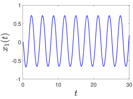
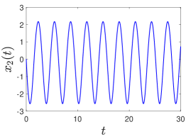
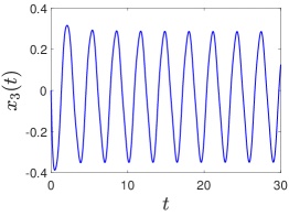
Figure 1: The components $x_{1}(t)=I_{L}(t)$, $x_{2}(t)=U_{L}(t)$ and $x_{3}(t)=I_{\varphi}(t)$ of the numerical solution

For $U(t)=(t+1)$, $I(t)=3(t+1)^{-1}$, $L(t)=10^{-1}+(t+1)^{-1}$, $R_{L}(t)=e^{-t}$, $R(t)=2+\cos t$, the functions $\varphi$, $\varphi_{L}$ of the form (69) where $a=b=1$ and $k=m=2$, and the consistent initial values $t_{0}=0$, $x_{0}=(0,37,3)^{\mathop{\mathrm{T}}}$, the components of the numerical solution are plotted in Fig. 2. In this case, an exact solution is global, but it can be unbounded, since the conditions of the Lagrange stability are not fulfilled.

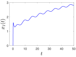
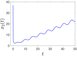
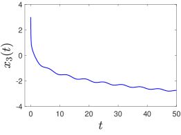
Figure 2: The components $x_{1}(t)=I_{L}(t)$, $x_{2}(t)=U_{L}(t)$ and $x_{3}(t)=I_{\varphi}(t)$ of the numerical solution

Further, consider the case when the function $U(t)$ is continuous, but not differentiable. Let the voltage $U(t)$ have the sawtooth shape (see Fig. 3)

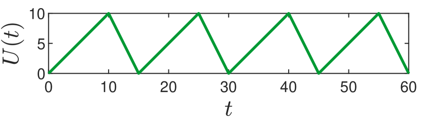
Figure 3: The voltage $U(t)$

$U(t)=\!\begin{cases}t-15\,k,&t\in[15\,k,10+15\,k],\;k\in\{0\}\cup{\mathbb{N}},\\ 30(k+1)-2t,&t\in[15\,k,10+15\,k,15+15\,k],\;k\in\{0\}\cup{\mathbb{N}}.\end{cases}$

Also, let ${I(t)=\sin(2t-\pi)}$, ${L(t)=10^{-1}+(t+1)^{-1}}$, ${R_{L}(t)=3+0.5\sin(2t)}$, $R{(t)=1+0.5\sin(2t)}$, and $\varphi,\,\varphi_{L}$ have the form (69) where $a=3$, $b=4$ and $k=m=2$. In this case, the DAE (1), (66) is Lagrange stable. The numerical solution for this case was obtained by both methods for $t_{0}=0$ and $x_{0}=(0,0,0)^{T}$. Its components obtained by method 1 are displayed in Fig. 4.

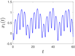
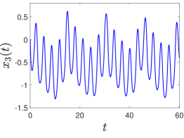
Figure 4: The numerical solution components $x_{1}(t)=I_{L}(t)$, $x_{2}(t)=U_{L}(t)$ and $x_{3}(t)=I_{\varphi}(t)$

The analysis of the obtained numerical solutions shows that the results of the numerical experiments are consistent with the results of the theoretical analysis of the DAE (1), (66).

3.2 Example 2: Analysis of a mathematical model of the electrical circuit dynamics

3.2.1 Theoretical analysis of the mathematical model of the electrical circuit dynamics

Consider an electrical circuit whose diagram is given in Fig. 5 (reference directions for currents and voltages across the circuit elements coincide). The global solvability of the mathematical model (1), (73) (see below) describing the dynamics of the circuit was studied in (Fil.DE-2, , Section 5). In the present section, we provide the conditions for the existence and uniqueness, as well as for the boundedness, of a global solution of the IVP for the DAE (1), (73) with the initial condition (3) both in the general case and in the particular cases for which approximate solutions are found using the obtained numerical methods (see Section 3.2.2). Here we use the theorems and propositions from Appendix.

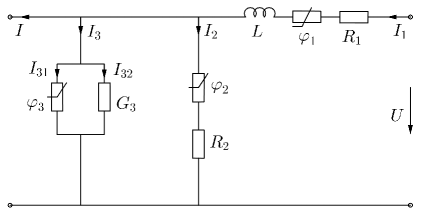
Figure 5: The electric circuit diagram

An inductance $L(t)$, a conductance $G_{3}(t)$ and resistances $R_{1}(t)$, $R_{2}(t)$, $\varphi_{1}(I_{1})$, $\varphi_{2}(I_{2})$ and $\varphi_{3}(I_{31})$ are given for the circuit. Inductance, resistance and conductance are given in henries (H), ohm ($\Omega$) and siemens (S), respectively.

We denote the unknown currents by $x_{1}(t)=I_{1}(t)$, $x_{2}(t)=I_{31}(t)$ and $x_{3}(t)=I_{2}(t)$ and in the sequel, for brevity, omit the dependence on $t$ in the notation for $x_{j}(t)$ ($j=1,2,3$). The mathematical model of the electrical circuit dynamics has the form of the system

$$\frac{d}{dt}[L(t)x_{1}]+R_{1}(t)x_{1}=U(t)-\varphi_{1}(x_{1})-\varphi_{3}(x_{2}),$$ (70)

$$x_{1}-x_{2}-x_{3}=I(t)+G_{3}(t)\varphi_{3}(x_{2}),$$ (71)

$$R_{2}(t)x_{3}=\varphi_{3}(x_{2})-\varphi_{2}(x_{3}),$$ (72)

which describes a transient process in the electrical circuit. The current $I(t)$ and voltage $U(t)$ are given. Having solved the obtained system, we find the currents $I_{1}(t)$, $I_{31}(t)$ and $I_{2}(t)$. The remaining currents and voltages in the circuit are uniquely expressed via the desired and given ones. The mathematical model (70)–(72) can be represented as the time-varying semilinear DAE (1), i.e.,

$\dfrac{d}{dt}[A(t)x]+B(t)x=f(t,x)$, where

$$x\!=\!\!\begin{pmatrix}\!x_{1}\\ x_{2}\\ x_{3}\!\end{pmatrix}\!,\,A(t)\!=\!\!\begin{pmatrix}L(t)&0&0\\ 0&0&0\\ 0&0&0\end{pmatrix}\!,\,B(t)\!=\!\!\begin{pmatrix}R_{1}(t)&0&0\\ 1&-1&-1\\ 0&0&R_{2}(t)\!\end{pmatrix}\!,\,f(t,x)\!=\!\!\begin{pmatrix}U(t)-\varphi_{1}(x_{1})-\varphi_{3}(x_{2})\\ I(t)+G_{3}(t)\varphi_{3}(x_{2})\\ \varphi_{3}(x_{2})-\varphi_{2}(x_{3})\!\end{pmatrix}\!.\!$$ (73)

We assume that $L,\,R_{1},\,R_{2}\in C^{1}([t_{+},\infty),{\mathbb{R}})$, $\varphi_{j}\in C^{1}({\mathbb{R}})$, $j=1,2,3$,  $I,\,U,\,G_{3}\in C([t_{+},\infty),{\mathbb{R}})$, and ${L(t),\,R_{1}(t),\,R_{2}(t),\,G_{3}(t)>0}$ for all ${t\in[t_{+},\infty)}$. Then $A,B\!\in\!C^{1}([t_{+},\infty),\mathrm{L}({\mathbb{R}}^{3}))$, $f\!\in\!C([t_{+},\infty)\times{\mathbb{R}}^{3},{\mathbb{R}}^{3})$, $\partial f/\partial x\!\in\!C([t_{+},\infty)\times{\mathbb{R}}^{3},\mathrm{L}({\mathbb{R}}^{3}))$, for each $t$ the pencil $\lambda A(t)+B(t)$ is regular and consequently there exists the resolvent $R(\lambda,t)=(\lambda A(t)+B(t))^{-1}$ (for regular points), and in addition the condition (4), where ${C_{1}(t)=\sqrt{2}\big{(}1+R_{2}^{-1}(t)\big{)}+1}$ and ${C_{2}(t)=L^{-1}(t)\big{(}1+R_{1}(t)\big{)}+1}$, holds for all ${t\in[t_{+},\infty)}$.

Using the formulas (15), we obtain the projection matrices $P_{j}(t)$, $Q_{j}(t)$ (6) (the algorithm for computing the projectors (6) by using (15) is given in Section 2) and then obtain the matrix $G(t)$ (8):

$P_{1}(t)\!=\!\begin{pmatrix}1&0&0\\ 1&0&0\\ 0&0&0\end{pmatrix}\!\!,\;P_{2}(t)\!=\!\begin{pmatrix}0&0&0\\ -1&1&0\\ 0&0&1\end{pmatrix}\!\!,\;Q_{1}(t)\!=\!\begin{pmatrix}1&0&0\\ 0&0&0\\ 0&0&0\end{pmatrix}\!\!,\;Q_{2}(t)\!=\!\begin{pmatrix}0&0&0\\ 0&1&0\\ 0&0&1\end{pmatrix}\!\!,\;G(t)\!=\!\!\begin{pmatrix}L(t)&0&0\\ 1&-1&-1\\ 0&0&R_{2}(t)\end{pmatrix}\!.$

Hence, the vector $x$ has the components (projections)

$x_{p_{1}}(t)=P_{1}(t)x=(x_{1},x_{1},0)^{\mathop{\mathrm{T}}}=:x_{p_{1}}$, $x_{p_{2}}(t)=P_{2}(t)x=(0,x_{2}-x_{1},x_{3})^{\mathop{\mathrm{T}}}=:x_{p_{2}}.$

Denote ${z=x_{1}}$, ${u=x_{2}-x_{1}}$, ${w=x_{3}}$, then ${x_{p_{1}}=(z,z,0)^{\mathop{\mathrm{T}}}}$, ${x_{p_{2}}=(0,u,w)^{\mathop{\mathrm{T}}}}$.

The consistency condition $(t,x)\in L_{t_{+}}$ (see Remark 1) holds if $t$ and $x_{i}$, $i=1,2,3$, satisfy the algebraic equations (71), (72). Using the above notation, we can rewrite the system (71), (72) as $u=-I(t)-G_{3}(t)\,\varphi_{3}(u+z)-w$,  $w=R_{2}^{-1}(t)\,[\varphi_{3}(u+z)-\varphi_{2}(w)]$ and transform it to the form

$$w=-I(t)-u-G_{3}(t)\,\varphi_{3}(u+z),$$ (74)

$$u=\psi(t,z,u),\quad\text{where}$$ (75)

$$\psi(t,z,u)=-I(t)-\left(G_{3}(t)+R_{2}^{-1}(t)\right)\varphi_{3}(u+z)+R_{2}^{-1}(t)\,\varphi_{2}\big{(}-I(t)-u-G_{3}(t)\,\varphi_{3}(u+z)\big{)}.$$ (76)

The derivation of the constraints on the functions in the DAE (1), (73), under which the conditions of Theorems 3.1 and 3.2 on the DAE global solvability are satisfied, is described in detail in (Fil.DE-2, , Section 5). The below conditions for the existence and uniqueness of a global solution of the IVP (1), (73), (3) were obtained based on these results.

Global solvability of the mathematical model (1), (73) of the electrical circuit dynamics. By Theorem 3.1, for each initial point $(t_{0},x_{0})\in[t_{+},\infty)\times{\mathbb{R}}^{3}$, where $x_{0}=(x_{0,1},x_{0,2},x_{0,3})^{\mathop{\mathrm{T}}}$, for which the equalities (71) and (72) (i.e., the consistency condition $(t_{0},x_{0})\in L_{t_{+}}$) hold, there exists a unique global solution of the DAE (1), (73) satisfying the initial condition (3)  if the following conditions are fulfilled:

$$L,\,R_{1},\,R_{2}\in C^{1}([t_{+},\infty),{\mathbb{R}}) I,\,U,\,G_{3}\in C([t_{+},\infty),{\mathbb{R}}) \varphi_{j}\in C^{1}({\mathbb{R}}) j=1,2,3$$,  ,  , , and

$${L(t),\,R_{1}(t),\,R_{2}(t),\,G_{3}(t)>0} t\in[t_{+},\infty)$$ for all ; (77)

for each $$t\in[t_{+},\infty) z\in{\mathbb{R}} u\in{\mathbb{R}}$$ and each there exists a unique such that (75) holds; (78)

for each $$t_{*}\in[t_{+},\infty) z_{*},\,u_{*},\,w_{*}\in{\mathbb{R}}$$ and each which satisfy (74), (75), the relation

$$\varphi^{\prime}_{3}(u_{*}+z_{*})+\big{[}\varphi^{\prime}_{2}(w_{*})+R_{2}(t_{*})\big{]}\big{[}1+G_{3}(t_{*})\,\varphi^{\prime}_{3}(u_{*}+z_{*})\big{]}\neq 0$$  holds; (79)

there exists a number $$R>0 -\big{(}\varphi_{1}(z)+\varphi_{3}(u+z)\big{)}z\leq R_{1}(t)z^{2}$$ such that 

for any $$t\in[t_{+},\infty) z,\,u\in{\mathbb{R}} |z|\geq R$$, satisfying (75) and . (80)

By Theorem 3.2, a similar statement holds if the above conditions are satisfied with the following changes: the condition (78) does not contain the requirement that $u$ be unique;  the condition (79) is replaced by the following:

$$\text{\emph{for each $t_{*}\in[t_{+},\infty)$, each $z_{*}\in{\mathbb{R}}$ and each $u_{*}^{j},\,w_{*}^{j}\in{\mathbb{R}}$, $j=1,2$, satisfying \eqref{NestElSyst2*}, \eqref{NestElSyst3*}}}\\ \text{\emph{the relation $\varphi^{\prime}_{3}(u_{2}+z_{*})+\big{[}\varphi^{\prime}_{2}(w_{2})+R_{2}(t_{*})\big{]}\big{[}1+G_{3}(t_{*})\,\varphi^{\prime}_{3}(u_{1}+z_{*})\big{]}\neq 0$ holds}}\\ \text{\emph{for any $u_{k}\in[u_{*}^{1},u_{*}^{2}]$, $w_{k}\in[w_{*}^{1},w_{*}^{2}]$, $k=1,2$}}$$ (81)

(obviously, this condition is satisfied in the case if the relation present in it holds for each $t_{*}\in[t_{+},\infty)$, each $z_{*}\in{\mathbb{R}}$ and each $u_{k},\,w_{k}\in{\mathbb{R}}$, $k=1,2$).

The global solvability conditions mentioned above can be weakened by using Proposition 1 (see Appendix).

Below, examples of the functions that satisfy the presented conditions are considered and certain changes of these conditions are discussed.

The conditions (78), (79), as well as (81), hold if the functions $\varphi_{2}$, $\varphi_{3}$ are increasing (nondecreasing) on ${\mathbb{R}}$, for example:

$$\varphi_{2}(y)=a\,y^{2k-1},\;\varphi_{3}(y)=b\,y^{2m-1}\;\text{ or }\;\varphi_{2}(y)=a\,y^{\frac{1}{2k-1}},\;\varphi_{3}(y)=b\,y^{\frac{1}{2m-1}},\;a,\,b>0,\;k,\,m\in\mathbb{N},$$ (82)

or if they have the form (83) and the inequality (84) is satisfied:

$$\varphi_{2}(y)=a\sin y,\;\varphi_{3}(y)=b\sin y\quad\text{ or }\quad\varphi_{2}(y)=a\cos y,\;\varphi_{3}(y)=b\cos y,\qquad a,\,b\in{\mathbb{R}},$$ (83)

$$G_{3}(t)|b|+R_{2}^{-1}(t)(|a|+|b|+G_{3}(t)|a|\,|b|)<1,\quad t\in[t_{+},\infty).$$ (84)

Note that if $\varphi_{2}$, $\varphi_{3}$ have the form (82), then the mapping $\psi(t,z,u)$ (76) is not globally contractive with respect to $u$ (in general, it does not satisfy the global Lipschitz condition in $u$ and $z$) for $k,m\geq 2$ and any $G_{3}(t)$, $R_{2}(t)$, $a$ and $b$, and hence the condition (98) (see Appendix) is not fulfilled. Obviously, if $\psi(t,z,u)$ is globally contractive with respect to $u$ for any $t$, $z$, i.e., there exists a constant $\alpha<1$ such that

$$\big{|}\psi(t,z,u_{1})-\psi(t,z,u_{2})\big{|}\leq\alpha|u_{1}-u_{2}|,\;\;u_{1},\,u_{2}\in{\mathbb{R}},$$ (85)

for each $t\in[t_{+},\infty)$ and each $z\in{\mathbb{R}}$, then the condition (78) holds.

If we take into account that $t_{*}$, $z_{*}$, $u_{*}$, $w_{*}$ satisfy (74), i.e., $w_{*}=-I(t_{*})-u_{*}-G_{3}(t_{*})\varphi_{3}(u_{*}+z_{*})$, but disregard the equality (75), then the condition (79) takes the following form:

for each $t_{*}\in[t_{+},\infty)$ and each $z_{*},\,u_{*}\in{\mathbb{R}}$ the relation $\dfrac{\partial\psi}{\partial u}(t_{*},z_{*},u_{*})\neq-1$ holds.

The conditions (78), (79) ensure the fulfillment of conditions 1, 2 of Theorem 3.1;  (78) without the requirement for $u$ to be unique and (81) ensure the fulfillment of conditions 1, 2 of Theorem 3.2. Instead of conditions 1, 2 of Theorem 3.1 or Theorem 3.2 one can use the condition (98) of Proposition 2 (see Appendix) which is satisfied if there exists a constant $\alpha<1$ such that

$$G_{3}(t)\,\big{|}\varphi_{3}(u_{1}+z)-\varphi_{3}(u_{2}+z)\big{|}+R_{2}^{-1}(t)\big{|}\varphi_{3}(u_{1}+z)-\varphi_{3}(u_{2}+z)-\varphi_{2}(w_{1})+\varphi_{2}(w_{2})\big{|}\leq\\ \leq\alpha\sqrt{|u_{1}-u_{2}|^{2}+|w_{1}-w_{2}|^{2}}$$ (86)

for any $t\in[t_{+},\infty)$, $z\in{\mathbb{R}}$ and $u_{i},\,w_{i}\in{\mathbb{R}}$, $i=1,2$, that is, the nonlinear function in the “algebraic part” of the DAE is a globally contractive with respect to $x_{p_{2}}$ for any $t$, $x_{p_{1}}$. However, this condition is more restrictive. If we take into account that the graph of a solution $x(t)$ must lie in the manifold $L_{t_{+}}$ and, therefore, $t$, $z$, $u$, $w$ are related by the equalities (74), (75), then, using these equalities, we can transform the inequality (86) so that it will be similar to (85).

To derive the condition (80), the function $V(t,x_{p_{1}}(t))$ of the form (99) with a time-invariant operator $H$, i.e., $V(t,x_{p_{1}}(t))\equiv\big{(}Hx_{p_{1}}(t),x_{p_{1}}(t)\big{)}$, where $H=0.5\,I_{{\mathbb{R}}^{3}}$, was chosen. Then condition 3 of Theorem 3.1 (the same condition is present in Theorem 3.2) is satisfied if there exist functions ${\tilde{U}\in C((0,\infty),(0,\infty))}$ and ${k\in C([t_{+},\infty),{\mathbb{R}})}$ such that ${\int\limits_{{\textstyle v}_{0}}^{\infty}\big{(}\tilde{U}(v)\big{)}^{-1}\,dv=\infty}$ (${v_{0}>0}$) and for some $R>0$ the inequality

$$2L^{-1}(t)\big{[}-(L^{\prime}(t)+R_{1}(t))z^{2}+U(t)z-\big{(}\varphi_{1}(z)+\varphi_{3}(u+z)\big{)}z\big{]}\leq k(t)\,\tilde{U}(z^{2})$$ (87)

holds for all $t\!\in\![t_{+},\infty)$, $z,u\!\in\!{\mathbb{R}}$ satisfying (75) and $|z|\!\geq\!R$. It is readily verified that the condition (87), where $k(t)\!=\!2L^{-1}(t)\big{(}|L^{\prime}(t)|+|U(t)|\big{)}$ and $\tilde{U}(v)\!=\!v$, is satisfied if (80) holds. The specified functions $k(t)$, $\tilde{U}(v)$ are also used to obtain conditions for the Lagrange stability of the DAE (1), (73).

Global solvability of the mathematical model (1), (73) in some particular cases.

I. Consider the functions

$$\varphi_{1}(y)=c\,y^{2l-1},\quad\varphi_{2}(y)=a\,y^{2k-1},\quad\varphi_{3}(y)=b\,y^{2m-1},\quad a,\,b,\,c>0,\quad k,\,m,\,l\in\mathbb{N},$$ (88)

where $\varphi_{2}$, $\varphi_{3}$ from (82).  The functions (88) satisfy (80) if $\sup\limits_{t\in[t_{+},\infty)}\!|I(t)|<\infty$, $\inf\limits_{t\in[t_{+},\infty)}\!R_{2}(t)=K_{0}>0$ and ${m\leq l}$.

Thus, if $\varphi_{j}$, $j=1,2,3$, have the form (88), where ${m\leq l}$, and, in addition, $L,R_{1},R_{2}\in C^{1}([t_{+},\infty),{\mathbb{R}})$,  $I,U,G_{3}\in C([t_{+},\infty),{\mathbb{R}})$,  $L(t),R_{1}(t),G_{3}(t)>0$ for $t\in[t_{+},\infty)$,  $\sup\limits_{t\in[t_{+},\infty)}|I(t)|<\infty$ and $\inf\limits_{t\in[t_{+},\infty)}R_{2}(t)=K_{0}>0$, then for each initial point $(t_{0},x_{0})\in[t_{+},\infty)\times{\mathbb{R}}^{3}$ satisfying (71), (72) there exists a unique global solution of the IVP (1), (73), (3).

II. Now consider the functions

$$\varphi_{1}(y)=c\sin y,\quad\varphi_{2}(y)=a\sin y,\quad\varphi_{3}(y)=b\sin y,\quad a,\,b,\,c\in{\mathbb{R}},$$ (89)

where $\varphi_{2}$, $\varphi_{3}$ from (83) and we can replace sines by cosines in (89).  For the functions (89) the condition (80) holds if ${\inf\limits_{t\in[t_{+},\infty)}R_{1}(t)=R_{*}>0}$. Notice that for the functions (83) condition 1 of Theorem 3.2 is always satisfied.

Thus, if $\varphi_{j}$, $j=1,2,3$, have the form (89), and, in addition, $L,R_{1},R_{2}\in C^{1}([t_{+},\infty),{\mathbb{R}})$,  $I,U,G_{3}\in C([t_{+},\infty),{\mathbb{R}})$,  $L(t),R_{2}(t),G_{3}(t)>0$ for $t\in[t_{+},\infty)$,  the functions $\varphi_{2}$, $\varphi_{3}$, $G_{3}$ and $R_{2}$ satisfy the condition (84), and $\inf\limits_{t\in[t_{+},\infty)}R_{1}(t)=R_{*}>0$, then for each initial point $(t_{0},x_{0})\in[t_{+},\infty)\times{\mathbb{R}}^{3}$ satisfying (71), (72) there exists a unique global solution of the IVP (1), (73), (3).

Lagrange stability of the mathematical model (1), (73).  By Theorem 3.3 (see Appendix), the DAE (1), (73) is Lagrange stable if the above conditions (77)–(80) are fulfilled and in addition ${\int\limits_{t_{+}}^{\infty}\!L^{-1}(t)\big{(}|L^{\prime}(t)|+|U(t)|\big{)}dt\!<\!\infty}$ (this integral converges if $\int\limits_{t_{+}}^{\infty}L^{-1}(t)|U(t)|dt\!<\!\infty$ and $\mathop{\lim}\limits_{t\to\infty}\!L(t)=\tilde{L}\!<\!\infty$, $\tilde{L}\neq 0$) and condition 4a, or 4b, or 4c from Theorem 3.3 holds. Notice that condition 4a of Theorem 3.3 is a consequence of condition 4b.

Condition 4a of Theorem 3.3 as well as condition 4b holds if $[I(t)+G_{3}(t)\varphi_{3}(x_{2})+R_{2}^{-1}(t)(\varphi_{3}(x_{2})-\varphi_{2}(x_{3}))]^{2}+[R_{2}^{-1}(t)(\varphi_{3}(x_{2})-\varphi_{2}(x_{3}))]^{2}\leq K_{M_{*}}=const$ for all $t\!\in\![t_{+},\infty)$, $x_{2},\,x_{3}\!\in\!{\mathbb{R}}$ and $|x_{1}|\leq M_{*}$ (where $M_{*}$ is an arbitrary constant) satisfying the equalities (71), (72). These conditions are fulfilled, for example, if  ${\sup\limits_{t\in[t_{+},\infty)}\!|I(t)|\!<\!\infty}$,  $\sup\limits_{t\in[t_{+},\infty)}\!G_{3}(t)\!<\!\infty$,  $\sup\limits_{t\in[t_{+},\infty)}\!R_{2}^{-1}(t)\!<\!\infty$,  $\sup\limits_{x_{2}\in{\mathbb{R}}}\!|\varphi_{3}(x_{2})|\!<\!\infty$ and $\sup\limits_{x_{3}\in{\mathbb{R}}}\!|\varphi_{2}(x_{3})|\!<\!\infty.$

Choose $\tilde{x}_{p_{2}}(t_{*})=\tilde{x}_{p_{2}}=(0,\tilde{x}_{2}-x_{1}^{*},\tilde{x}_{3})^{\mathop{\mathrm{T}}}=(0,\tilde{u},\tilde{w})^{\mathop{\mathrm{T}}}=0$. Then it is easily verified that condition 4c of Theorem 3.3 is satisfied if, for example, the following conditions are satisfied:  for each $t_{*}\in[t_{+},\infty)$ and each $z_{*},\,u_{*},\,w_{*}\in{\mathbb{R}}$ satisfying (74), (75) and for any $\lambda_{1},\lambda_{2}\in(0,1]$ the relation ${\varphi^{\prime}_{3}(\lambda_{2}u_{*}+z_{*})+\big{[}\varphi^{\prime}_{2}(\lambda_{2}w_{*})+R_{2}(t_{*})\big{]}\big{[}1+G_{3}(t_{*})\,\varphi^{\prime}_{3}(\lambda_{1}u_{*}+z_{*})\big{]}\neq 0}$ holds (i.e., the relation from the condition (81), where $u_{i}=\lambda_{i}u_{*}$, $i=1,2$, and $w_{2}=\lambda_{2}w_{*}$, holds); for all $t_{*}\!\in\![t_{+},\infty)$, $z_{*},u_{*},w_{*}\!\in\!{\mathbb{R}}$ satisfying (74), (75) it holds that $|I(t_{*})|\!<\!\infty$, $G_{3}(t_{*})\!<\!\infty$, $R_{2}^{-1}(t_{*})\!<\!\infty$, $|\varphi_{2}(w_{*})|\!<\!\infty$ and $|\varphi_{3}(u_{*}\!+\!z_{*})|\!\leq\!K_{1}(z_{*})\!<\!\infty$, where $K_{1}(z_{*})\!=\!K_{1}^{*}$ is some constant for each fixed $z_{*}$.

3.2.2 Numerical analysis of the mathematical model of the electrical circuit dynamics

In this section, we present the plots of numerical solutions of the DAE (1), (73) describing the electrical circuit dynamics (see Section 3.2.1) for such parameters of the electric circuit (i.e., the functions $I(t)$, $U(t)$, $G_{3}(t)$, $L(t)$, $R_{1}(t)$, $R_{2}(t)$, $\varphi_{1}(x_{1})$, $\varphi_{2}(x_{3})$ and $\varphi_{3}(x_{2})$) for which there exists a unique global solution of the IVP (1), (73), (3), as well as the conditions of Theorems 2.1, 2.2 or Remarks 2, 3 on the convergence of the methods hold.

Consider the particular case when $\varphi_{i}$, $i=1,2,3$, have the form (88), where $k=m=l=2$, i.e.,

$$\varphi_{1}(y)=c\,y^{3},\quad\varphi_{2}(y)=a\,y^{3},\quad\varphi_{3}(y)=b\,y^{3},\quad a,b,c>0,\quad y\in{\mathbb{R}}.$$ (90)

Let $L,\,R_{1},\,R_{2}\in C^{1}([t_{+},\infty),{\mathbb{R}})$,  $I,\,U,\,G_{3}\in C([t_{+},\infty),{\mathbb{R}})$,  $L(t),\,R_{1}(t),\,G_{3}(t)>0$ for all $t\in[t_{+},\infty)$,  ${\sup\limits_{t\in[t_{+},\infty)}|I(t)|<\infty}$ and $\inf\limits_{t\in[t_{+},\infty)}R_{2}(t)=K_{0}>0$. Then, as shown in Section 3.2.1, for each initial point $(t_{0},x_{0})\in[t_{+},\infty)\times{\mathbb{R}}^{3}$ satisfying the equalities (71), (72) there exists a unique global solution of the IVP for the DAE (1), (73), (90) with the initial condition (3).

Note that the equalities (71) and (72) can be transformed into the following form:

$$x_{3}=x_{1}-x_{2}-I(t)-G_{3}(t)\,\varphi_{3}(x_{2}),$$ (91)

$$x_{2}=x_{1}-I(t)-\left(G_{3}(t)+R_{2}^{-1}(t)\right)\varphi_{3}(x_{2})+R_{2}^{-1}(t)\,\varphi_{2}\big{(}x_{1}-x_{2}-I(t)-G_{3}(t)\,\varphi_{3}(x_{2})\big{)}$$ (92)

(recall that if $(t,x)$ satisfy (71), (72), then $(t,x)\in L_{t_{+}}$), and the condition (78) can be rewritten as follows: for each $t\in[t_{+},\infty)$ and each $x_{1}\in{\mathbb{R}}$ there exists a unique $x_{2}\in{\mathbb{R}}$ such that (92) holds. Consequently, by setting arbitrary initial values $t_{0}\in[t_{+},\infty)$ and $x_{0,1}\in{\mathbb{R}}$, one can always find a unique $x_{0,2}$ by the formula (92) and then find a unique $x_{0,3}$ by the formula (91) such that the initial point $(t_{0},x_{0})$, where $x_{0}=(x_{0,1},x_{0,2},x_{0,3})^{\mathop{\mathrm{T}}}$, will be consistent.  For example, in the particular case when $\varphi_{i}$ have the form (90), if $t_{+}=t_{0}=0$, $x_{0,1}=0$ and $I(t)$ is such that $I(0)=0$, then $t_{0}=0$, $x_{0}=(0,0,0)^{\mathop{\mathrm{T}}}$ are consistent initial values.

Recall that the components of a solution $x(t)=(x_{1}(t),x_{2}(t),x_{3}(t))^{\mathop{\mathrm{T}}}$ denote the functions of the currents, namely, $x_{1}(t)=I_{1}(t)$, $x_{2}(t)=I_{31}(t)$ and $x_{3}(t)=I_{2}(t)$.

Consider the case when $I(t)=(t+1)^{-1}-1$, $U(t)=(t+1)$, $G_{3}(t)=(t+1)^{2}$, $L(t)=500\,(t+1)^{-1}$, $R_{1}(t)=1+(t+1)^{-1}$, $R_{2}(t)=1-(t+1)^{-1}$ and $\varphi_{i}$, $i=1,2,3$, have the form (90) where $a=b=c=1$, and take the consistent initial values $t_{0}=0$, $x_{0}=(0,0,0)^{\mathop{\mathrm{T}}}$. The components of the computed solution are plotted in Fig. 6. As mentioned above, in all cases considered in this section, an exact solution is global, i.e., exists on $[t_{0},\infty)$.

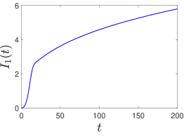
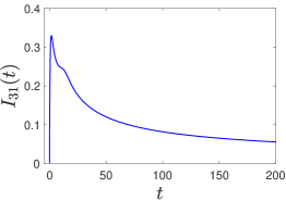
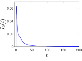
Figure 6: The components $x_{1}(t)=I_{1}(t)$, $x_{2}(t)=I_{31}(t)$ and $x_{3}(t)=I_{2}(t)$ of the numerical solution

In realistic problems of electrical engineering the inductance $L(t)$ can be very small, therefore, we take ${L(t)=10^{-3}}$. Choose the remaining parameters of the circuit and consistent initial values in the form ${R_{1}(t)=e^{-t}}$, $R_{2}(t)=5+e^{-t}$, $I(t)=\sin t$, $U(t)=(t+1)^{-1}$, $G_{3}(t)=(t+1)^{-1}$, (90) where $a=b=c=1$, and $t_{0}=0$, $x_{0}=(0,0,0)^{\mathop{\mathrm{T}}}$. Then we obtain the numerical solution plotted in Fig. 7.

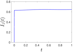
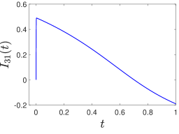
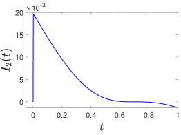
Figure 7: The components $x_{1}(t)=I_{1}(t)$, $x_{2}(t)=I_{31}(t)$ and $x_{3}(t)=I_{2}(t)$ of the numerical solution

Consider the case when the function $U(t)$ is not continuously differentiable, but only continuous. Take the voltage of the triangular shape (see Fig. 8):

Figure 8: The voltage $U(t)$

${U(t)=10-|t-10-20\,k|},\quad t\in[20\,k,20+20\,k],\quad k\in{\mathbb{N}}\cup\{0\}.$

In this case we use Remarks 2 and 3. Also, take $I(t)=(t+1)^{-1}-1$, $G_{3}(t)=(t+1)^{-1}$, $L(t)=10^{-1}+(t+1)^{-1}$, $R_{1}(t)=e^{-t}$, $R_{2}(t)=2+e^{-t}$, the functions $\varphi_{i}$ ($i=1,2,3$) of the form (90), where $a=b=c=1$, and the consistent initial values $t_{0}=0$, $x_{0}=(0,0,0)^{\mathop{\mathrm{T}}}$. The numerical solution for this case was obtained by both method 1 and method 2. The plots of its components obtained by method 2 are presented in Fig. 9.

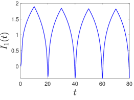
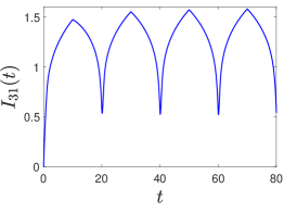
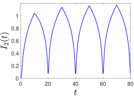
Figure 9: The numerical solution components $x_{1}(t)=I_{1}(t)$, $x_{2}(t)=I_{31}(t)$, $x_{3}(t)=I_{2}(t)$

Now, consider the case when $I(t)=(\ln(t+1)+1)^{-1}$, $U(t)=100(t+1)^{-2}$, $G_{3}(t)=(t+1)^{-1}$, $L(t)=(t+10)^{-1/2}+10^{-2}$, $R_{1}(t)=1+0.5\sin t$, $R_{2}(t)=3+0.5\sin t$ and

$\varphi_{1}(x_{1})=x_{1}^{5},\quad\varphi_{2}(x_{3})=(\cos x_{3})/3,\quad\varphi_{3}(x_{2})=(\cos x_{2})/3,$

In this case the DAE (1), (73) is Lagrange stable. Take the consistent initial values $t_{0}=0$, $x_{0}=(4/3,0,0)^{\mathop{\mathrm{T}}}$. The plots of the components of the numerical solution are given in Fig. 10.

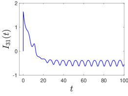
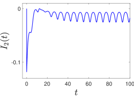
Figure 10: The numerical solution components $x_{1}(t)=I_{1}(t)$, $x_{2}(t)=I_{31}(t)$, $x_{3}(t)=I_{2}(t)$

Further, consider the particular case when $\varphi_{i}$, $i=1,2,3$, have the form (89), that is,

$\varphi_{1}(y)=c\sin y,\quad\varphi_{2}(y)=a\sin y,\quad\varphi_{3}(y)=b\sin y,\quad a,\,b,\,c\in{\mathbb{R}}.$

Let $L,R_{1},R_{2}\in C^{1}([t_{+},\infty),{\mathbb{R}})$,  $I,U,G_{3}\in C([t_{+},\infty),{\mathbb{R}})$,  $L(t),R_{2}(t),G_{3}(t)>0$ for $t\in[t_{+},\infty)$,  the functions $G_{3}(t)$, $R_{2}(t)$ and numbers $a$, $b$ satisfy the condition (84) and $\inf\limits_{t\in[t_{+},\infty)}R_{1}(t)=R_{*}>0$. Then, as shown in Section 3.2.1, for each initial point $(t_{0},x_{0})\in[t_{+},\infty)\times{\mathbb{R}}^{3}$ satisfying (71), (72) there exists a unique global solution of the DAE (1), (73), (89) with the initial condition (3). It is readily verified that $t_{0}=0$ and $x_{0}=(0,0,0)^{\mathop{\mathrm{T}}}$ are consistent initial values if $I(0)=0$.

For $I(t)=t$, $U(t)=t+1$, $G_{3}(t)=(t+1)^{-1}$, $L(t)=1$, $R_{1}(t)=2+e^{-t}$, $R_{2}(t)=0.1t+3$, $\varphi_{i}$ ($i=1,2,3$) of the form (89) where $a=1/3$, $b=-1/2$ and $c=10$, and the consistent initial values $t_{0}=0$, $x_{0}=(0,0,0)^{\mathop{\mathrm{T}}}$, the plots of the numerical solution are presented in Fig. 11.

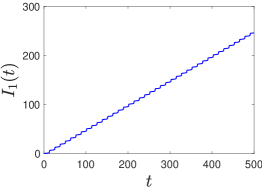
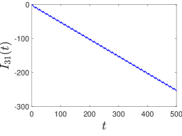
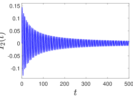
Figure 11: The components $x_{1}(t)=I_{1}(t)$, $x_{2}(t)=I_{31}(t)$ and $x_{3}(t)=I_{2}(t)$ of the numerical solution

Consider the case when the DAE is Lagrange stable. Choose $I(t)=\sin t$, $U(t)=(t+1)^{-5/2}$, $G_{3}(t)=(t+1)^{-1}$, $L(t)=10^{-1}+(t+1)^{-1}$, $R_{1}(t)=1+e^{-t}$, $R_{2}(t)=0.5\cos t+3$,  $\varphi_{i}$ ($i=1,2,3$) of the form (89) where $a=1/3$, $b=-1/2$, $c=5$. Then the conditions of the Lagrange stability, specified in Section 3.2.1, hold. The components of the solution computed for the consistent initial values $t_{0}\!=\!0$, $x_{0}\!=\!(0,0,0)^{\mathop{\mathrm{T}}}$ are plotted in Fig. 12.

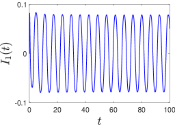
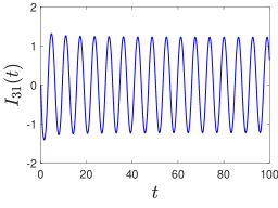
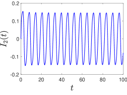
Figure 12: The components $x_{1}(t)=I_{1}(t)$, $x_{2}(t)=I_{31}(t)$ and $x_{3}(t)=I_{2}(t)$ of the numerical solution

The obtained numerical solutions show that the results of the theoretical research of the mathematical model considered in Section 3.2.1 are consistent with the results of the numerical experiments.

We can conclude that methods 1, 2 are easy to implement, effective enough, and enable to carry out the numerical analysis of the global dynamics of mathematical models described by time-varying semilinear DAEs or the corresponding descriptor systems. The features and advantages of the methods were discussed in Section 2.

3.3 Comparison of methods 1 and 2

Consider the time-varying semilinear DAE (1) (where for brevity we omit the dependence on $t$ in the notation of the variable vector $x(t)$) with $A(t)$, $B(t)$, $f(t,x)$ and $x$ of the form (73). The physical interpretation of this equation is given in Section 3.2.1. Recall that the variables denote currents, namely, $x_{1}=I_{1}$, $x_{2}=I_{31}$ and $x_{3}=I_{2}$. To compare method 1 (the simple combined method (18)–(21)) and method 2 (the combined method with recalculation (47)–(52)), we consider the following example: $I(t)=\sin t$, $U(t)=(t+1)^{-1}$, $G_{3}(t)=(t+1)^{-1}$, $L(t)=500$, $R_{1}(t)=e^{-t}$, $R_{2}(t)=2+e^{-t}$, $\varphi_{1}(x_{1})=x_{1}^{3}$, $\varphi_{2}(x_{3})=x_{3}^{3}$, $\varphi_{3}(x_{2})=x_{2}^{3}$, and $t_{0}=0$, $x_{0}=(0,0,0)^{\mathop{\mathrm{T}}}$.

Figures 13 and 14 illustrating how the plots of the components $x_{1}(t)=I_{1}(t)$,  $x_{2}(t)=I_{31}(t)$ of a solution $x(t)=(x_{1}(t),x_{2}(t),x_{3}(t))^{\mathop{\mathrm{T}}}$, obtained by methods 1 and 2 respectively, changes with the mesh refinement (${h=0.1,\,0.01,\,0.001}$) show that the numerical solutions approach each other when decreasing a step size, and hence methods 1 and 2 converge, at that, the solutions obtained by method 2 approach each other faster. To show more clearly that the numerical solutions obtained by method 2 for the step sizes $h=0.1$, $h=0.01$ and $h=0.001$ approach each other (when decreasing the step size) faster than those obtained by method 1, the plots of the components $x_{1}(t)=I_{1}(t)$, $x_{2}(t)=I_{31}(t)$, obtained by both methods, are displayed on an enlarged scale in Fig. 15, 16. Table 1 gives the same result. Thus, it is shown that method 2 converges faster than method 1.

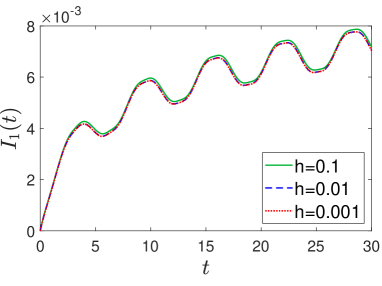
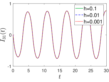
Figure 13: The solution components $x_{1}(t)=I_{1}(t)$ and $x_{2}(t)=I_{31}(t)$ obtained by method 1 with the step sizes ${h=0.1,\,0.01,\,0.001}$

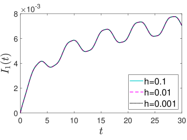
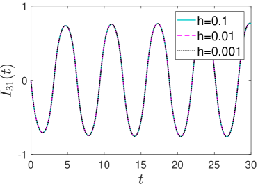
Figure 14: The solution components $x_{1}(t)=I_{1}(t)$ and $x_{2}(t)=I_{31}(t)$ obtained by method 2 with the step sizes ${h=0.1,\,0.01,\,0.001}$

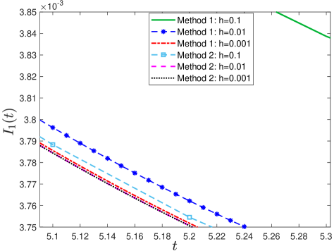
Figure 15: The plots of $x_{1}(t)=I_{1}(t)$ (on an enlarged scale) obtained by methods 1 and 2 with the step sizes $h=0.1,\,0.01,\,0.001$

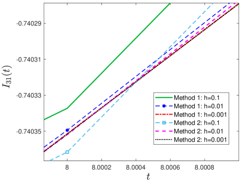
Figure 16: The plots of $x_{2}(t)=I_{31}(t)$ (on an enlarged scale) obtained by methods 1 and 2 with the step sizes $h=0.1,\,0.01,\,0.001$

Table 1: The values of the solution component $x_{1}(t)=I_{1}(t)$ obtained by methods 1 and 2 at $t=0.2,\,0.4,\,0.6,\,0.8$

	$I_{1}(0.2)$	$I_{1}(0.4)$	$I_{1}(0.6)$	$I_{1}(0.8)$
$h$	Method 1 Method 2	Method 1 Method 2	Method 1  Method 2	Method 1  Method 2​​​
$10^{-1}$​​	3.8198e-04  3.6601e-04	7.0802e-04  6.8362e-04	0.001006  9.7880e-04	0.001296  0.001268​​
$10^{-2}$​​	3.6690e-04  3.6530e-04	6.8447e-04  6.8202e-04	0.000979  0.000976	0.001268  0.001265​​
$10^{-3}$​​	3.6546e-04  3.6530e-04	6.8224e-04  6.8200e-04	0.000977  0.000976	0.001265  0.001265​​

As stated in Theorems 2.1, 2.2, methods 1 and 2 have the first and second order of accuracy respectively, but at the same time method 2 requires greater smoothness for the functions in the equation, namely, methods 1 and 2 require that $A,B\!\in\!C^{2}([t_{0},T],\mathrm{L}({\mathbb{R}}^{n}))$, $C_{2}\!\in\!C^{2}([t_{0},T],(0,\infty))$, $f\!\in\!C^{1}([t_{0},T]\times{\mathbb{R}}^{n},{\mathbb{R}}^{n})$ and $A,B\!\in\!C^{3}([t_{0},T],\mathrm{L}({\mathbb{R}}^{n}))$, $C_{2}\!\in\!C^{3}([t_{0},T],(0,\infty))$, $f\!\in\!C^{2}([t_{0},T]\times{\mathbb{R}}^{n},{\mathbb{R}}^{n})$ respectively. However, if $A,B\!\in\!C^{1}([t_{+},\infty),\mathrm{L}({\mathbb{R}}^{n}))$, $C_{2}\!\in\!C^{1}([t_{+},\infty),(0,\infty))$ and $f\!\in\!C([t_{+},\infty)\times{\mathbb{R}}^{n},{\mathbb{R}}^{n})$ is such that $\partial f/\partial x$ is continuous on $[t_{+},\infty)\times{\mathbb{R}}^{n}$, then the methods also converge, as stated in Remarks 2, 3, and method 2 still converges faster. The rate of convergence of method 2 increases mainly due to the faster convergence of the component $x_{p_{1}}(t)$, since in method 1 the method having the first order of accuracy is applied to the “differential part” of the DAE (to the DE), and in method 2, due to recalculation, it has the second order of accuracy. The Newton-type method with respect to $x_{p_{2}}(t)$ (which in general has the second order of accuracy if functions in the equation are sufficiently smooth) is applied to the “algebraic part” of the DAE (to the AE) and the rate of convergence of the component $x_{p_{2}}(t)$ in method 2 increases due to the fact that the refined value of $x_{p_{1}}(t)$ is used in its recalculation. This is shown in the proofs of Theorems 2.1 and 2.2 as well as in the figures above. The numerical experiments shown in Section 3 confirm the results of the above comparative analysis.

Appendix: Existence, uniqueness and boundedness of global solutions of time-varying semilinear DAEs

Below we give definitions Fil.DE-1 ; Fil.MPhAG that will be needed to formulate further results.

A solution $x(t)$ of the IVP (1), (3) is called global if it exists on the interval $[t_{0},\infty)$. A solution $x(t)$ of the IVP (1), (3) is called Lagrange stable if it is global and bounded, i.e., $x(t)$ exists on $[t_{0},\infty)$ and $\sup\limits_{t\in[t_{0},\infty)}\|x(t)\|<\infty$. A solution $x(t)$ of the IVP (1), (3) is called Lagrange unstable (a solution has a finite escape time or is blow-up in finite time) if it exists on some finite interval $[t_{0},T)$ and is unbounded, i.e., there exists $T>t_{0}$ ($T<\infty$) such that $\mathop{\lim}\limits_{t\to T-0}\|x(t)\|=\infty$.

The equation (1) is called Lagrange stable (Lagrange unstable) for the initial point $(t_{0},x_{0})$ if the solution of the IVP (1), (3) is Lagrange stable (Lagrange unstable) for this initial point.  The equation (1) is called Lagrange stable (Lagrange unstable) if each solution of the IVP (1), (3) is Lagrange stable (Lagrange unstable), that is, the equation is Lagrange stable (Lagrange unstable) for each consistent initial point.

Similar definitions hold for the DAE (2) (the IVP (2), (3)).

Recall the following classical definitions. Let $D\!\subset\!{\mathbb{R}}^{n}$ be a region containing the origin. A function $W\!\in\!C(D,{\mathbb{R}})$ is said to be positive definite if $W(x)>0$ for all $x\neq 0$ and $W(0)=0$. A function $V\!\in\!C([t_{+},\infty)\times D,{\mathbb{R}})$ is said to be positive definite if $V(t,0)\equiv 0$ and there exists a positive definite function $W\!\in\!C(D,{\mathbb{R}})$ such that $V(t,x)\geq W(x)$ for all $x\neq 0$, $t\!\in\![t_{+},\infty)$.

The existence, uniqueness and boundedness of global solutions of the DAEs (1) and (2). In what follows, the following notation will be used:

$$U_{R}^{c}(0)=\{z\in{\mathbb{R}}^{n}\mid\|z\|\geq R\}.$$

Theorem 3.1 (Global solvability of the DAE (1), (Fil.DE-1, , Theorem 2.1))

Let $f\in C([t_{+},\infty)\times{\mathbb{R}}^{n},{\mathbb{R}}^{n})$, $\partial f/\partial x\in C([t_{+},\infty)\times{\mathbb{R}}^{n},\mathrm{L}({\mathbb{R}}^{n}))$, $A,B\in C^{1}([t_{+},\infty),\mathrm{L}({\mathbb{R}}^{n}))$,  the pencil $\lambda A(t)+B(t)$ satisfy (4), where $C_{2}\in C^{1}([t_{+},\infty),(0,\infty))$, and the following conditions hold:

1. For each $t\in[t_{+},\infty)$ and each $x_{p_{1}}(t)\in X_{1}(t)$ there exists a unique $x_{p_{2}}(t)\in X_{2}(t)$ such that

   $$(t,x_{p_{1}}(t)+x_{p_{2}}(t))\in L_{t_{+}}.$$ (93)

2. For each $t_{*}\in[t_{+},\infty)$, each $x_{p_{1}}^{*}(t_{*})\in X_{1}(t_{*})$, and each $x_{p_{2}}^{*}(t_{*})\in X_{2}(t_{*})$ such that $(t_{*},x_{p_{1}}^{*}(t_{*})+x_{p_{2}}^{*}(t_{*}))\in L_{t_{+}}$, the operator $\Phi_{t_{*},x^{*}_{p_{1}}(t_{*}),x^{*}_{p_{2}}(t_{*})}$ defined by

   $$\Phi_{t_{*},x^{*}_{p_{1}}(t_{*}),x^{*}_{p_{2}}(t_{*})}=\!\left[\frac{\partial}{\partial x}\big{[}Q_{2}(t_{*})\,f\big{(}t_{*},x^{*}_{p_{1}}(t_{*})+x^{*}_{p_{2}}(t_{*})\big{)}\,\big{]}-B(t_{*})\right]\!P_{2}(t_{*})\colon X_{2}(t_{*})\to Y_{2}(t_{*}),$$ (94)

   is invertible.

3. There exist functions ${k\in C([t_{+},\infty),{\mathbb{R}})}$, ${U\in C(0,\infty)}$, a number ${R>0}$ and a positive definite function $V\in C^{1}\big{(}[t_{+},\infty)\times U_{R}^{c}(0),{\mathbb{R}}\big{)}$ such that ${\int\limits_{{\textstyle v}_{0}}^{\infty}\big{(}U(v)\big{)}^{-1}\,dv=\infty}$ ($v_{0}>0$ is some constant) and it holds that

   3.1.  ${V(t,z)\to\infty}$ uniformly in $t$ on each finite interval $[a,b)\subset[t_{+},\infty)$ as ${\|z\|\to\infty}$;

   3.2.  For all $t\in[t_{+},\infty)$, $x_{p_{1}}(t)\in X_{1}(t)$, $x_{p_{2}}(t)\in X_{2}(t)$ such that $(t,x_{p_{1}}(t)+x_{p_{2}}(t))\in L_{t_{+}}$ and ${\|x_{p_{1}}(t)\|\geq R}$, the following inequality holds:

   $$V^{\prime}_{\eqref{DAEsys2.1}}(t,x_{p_{1}}(t))\leq k(t)\,U\big{(}V(t,x_{p_{1}}(t))\big{)},$$ (95)

   where  $V^{\prime}_{\eqref{DAEsys2.1}}(t,x_{p_{1}}(t))=\dfrac{\partial V}{\partial t}(t,x_{p_{1}}(t))+\!\bigg{(}\dfrac{\partial V}{\partial z}(t,x_{p_{1}}(t)),\big{[}P^{\prime}_{1}(t)-G^{-1}(t)Q_{1}(t)\,[A^{\prime}(t)+B(t)]\big{]}x_{p_{1}}(t)+G^{-1}(t)Q_{1}(t)\,f\big{(}t,x_{p_{1}}(t)+x_{p_{2}}(t)\big{)}\bigg{)}$ is the derivative of $V$ along the trajectories of (12) (where ${x_{p_{1}}(t)\!=\!z(t)}$).

Then for each initial point $(t_{0},x_{0})\in L_{t_{+}}$ there exists a unique global solution of the IVP (1), (3).

The equation (12) can be written as ${x_{p_{1}}^{\prime}(t)=\Pi(t,x_{p_{1}}(t),x_{p_{2}}(t))}$, where $\Pi$ has the form (22), i.e., $\Pi(t,x_{p_{1}}(t),x_{p_{2}}(t))=\big{[}P^{\prime}_{1}(t)-G^{-1}(t)\,Q_{1}(t)\,[A^{\prime}(t)+B(t)]\,\big{]}x_{p_{1}}(t)+G^{-1}(t)\,Q_{1}(t)f\big{(}t,x_{p_{1}}(t)+x_{p_{2}}(t)\big{)}$.

Consider the equation

$$x_{p_{1}}^{\prime}(t)=\Pi_{\scriptscriptstyle T}(t,x_{p_{1}}(t),x_{p_{2}}(t)),\quad\Pi_{\scriptscriptstyle T}(t,x_{p_{1}}(t),x_{p_{2}}(t))=\begin{cases}\Pi(t,x_{p_{1}}(t),x_{p_{2}}(t)),&t\in[t_{+},T],\\ \Pi(T,x_{p_{1}}(T),x_{p_{2}}(T)),&t>T,\end{cases}$$ (96)

where $T>t_{+}$ is a parameter and the function $\Pi_{\scriptscriptstyle T}$ is the truncation of $\Pi$ over $t$.

Proposition 1

Theorem 3.1 remains valid if condition 3 is replaced by the following:

1. There exists a positive definite function $V\in C^{1}([t_{+},\infty)\times U_{R}^{c}(0),{\mathbb{R}})$ where ${R>0}$ is some number, a function ${U\in C(0,\infty)}$ satisfying the relation ${\int\limits_{{\textstyle v}_{0}}^{\infty}\big{(}U(v)\big{)}^{-1}\,dv=\infty}$ ($v_{0}>0$ is some constant), and for each ${T>0}$ there exists a number ${R_{\scriptscriptstyle T}\geq R}$ and a function $k_{\scriptscriptstyle T}\in C([t_{+},\infty),{\mathbb{R}})$ such that

   3.1.  ${V(t,z)\to\infty}$ uniformly in $t$ on each finite interval $[a,b)\subset[t_{+},\infty)$ as ${\|z\|\to\infty}$;

   3.2.  For all ${t\in[t_{+},\infty)}$, ${x_{p_{1}}(t)\in X_{1}(t)}$, ${x_{p_{2}}(t)\in X_{2}(t)}$ such that $(t,x_{p_{1}}(t)+x_{p_{2}}(t))\in L_{t_{+}}$ and $\|x_{p_{1}}(t)\|\geq R_{\scriptscriptstyle T}$, the following inequality holds:

   $V^{\prime}_{\eqref{DAEsys2.1-cut}}(t,x_{p_{1}}(t))\leq k_{\scriptscriptstyle T}(t)\,U\big{(}V(t,x_{p_{1}}(t))\big{)},$

   where $V^{\prime}_{\eqref{DAEsys2.1-cut}}(t,x_{p_{1}}(t))=\dfrac{\partial V}{\partial t}(t,x_{p_{1}}(t))+\bigg{(}\dfrac{\partial V}{\partial z}(t,x_{p_{1}}(t)),\,\Pi_{\scriptscriptstyle T}(t,x_{p_{1}}(t),x_{p_{2}}(t))\bigg{)}$ is the derivative of $V$ along the trajectories of the equation (96).

Proof

The proof of the above proposition is easily derived from the proof of Theorem 3.1 (see Fil.DE-1 ), since a solution of the equation (96) with the truncation coincides with the solution of the original equation with the same initial values on the interval $[t_{+},T]$ (where the right-hand sides of the equations coincide).

A system of $s$ pairwise disjoint projectors $\{\Theta_{k}\in\mathrm{L}(Z)\}_{k=1}^{s}$ (i.e., $\Theta_{i}\,\Theta_{j}=\delta_{ij}\,\Theta_{i}$) such that $\sum\limits_{k=1}^{s}\Theta_{k}=I_{Z}$, where $Z$ is an $s$-dimensional linear space and $I_{Z}$ is the identity operator in $Z$, is called an additive resolution of the identity in $Z$ (cf. RF1 ). An operator function $\Phi\colon D\to\mathrm{L}(W,Z)$, where $W$, $Z$ are $s$-dimensional linear spaces and $D\subset W$, is called basis invertible on an interval $J\subset D$ if for some additive resolution of the identity $\{\Theta_{k}\}_{k=1}^{s}$ in $Z$ and for any set of elements $\{w^{k}\}_{k=1}^{s}\subset J$ the operator $\Lambda=\sum\limits_{k=1}^{s}\Theta_{k}\Phi(w^{k})\in\mathrm{L}(W,Z)$ has an inverse $\Lambda^{-1}\in\mathrm{L}(Z,W)$ (cf. RF1 ). The basis invertibility of $\Phi$ on $J$ implies its invertibility on $J$, i.e., the invertibility of the operator $\Phi(w^{*})$ for each $w^{*}\in J$ . The converse is not true, except for the case when $W$, $Z$ are one-dimensional.

Theorem 3.2 (Global solvability of the DAE (1), (Fil.DE-1, , Theorem 2.2))

Theorem 3.1 remains valid if conditions 1, 2 are replaced by the following:

1. For each $t\in[t_{+},\infty)$ and each $x_{p_{1}}(t)\in X_{1}(t)$ there exists $x_{p_{2}}(t)\in X_{2}(t)$ such that (93).

2. For each $t_{*}\in[t_{+},\infty)$, each $x_{p_{1}}^{*}(t_{*})\in X_{1}(t_{*})$, and each $x_{p_{2}}^{i}(t_{*})\in X_{2}(t_{*})$ such that $(t_{*},x_{p_{1}}^{*}(t_{*})+x_{p_{2}}^{i}(t_{*}))\in L_{t_{+}}$, $i=1,2$, the operator function $\Phi_{t_{*},x^{*}_{p_{1}}(t_{*})}(x_{p_{2}}(t_{*}))$ defined by

   $$\Phi_{t_{*},x^{*}_{p_{1}}(t_{*})}\!\colon\!X_{2}(t_{*})\to\mathrm{L}(X_{2}(t_{*}),Y_{2}(t_{*})),\;\Phi_{t_{*},x^{*}_{p_{1}}(t_{*})}(x_{p_{2}}(t_{*}))\!=\!\!\bigg{[}\frac{\partial}{\partial x}\!\big{[}Q_{2}(t_{*})f\big{(}t_{*},x^{*}_{p_{1}}(t_{*})\!+\!x_{p_{2}}(t_{*})\big{)}\big{]}\!-\!B(t_{*})\bigg{]}\!P_{2}(t_{*}),\!\!$$ (97)

   is basis invertible on $[x_{p_{2}}^{1}(t_{*}),x_{p_{2}}^{2}(t_{*})]$.

Remark 5

Theorems 3.1 and 3.2 ensure the following smoothness for the components of a solution $x(t)$ of the DAE (1): $P_{1}(t)x(t)\in C^{1}([t_{0},\infty),{\mathbb{R}}^{n})$, $P_{2}(t)x(t)\in C([t_{0},\infty),{\mathbb{R}}^{n})$. If in these theorems $A,\,B\in C^{m+1}([t_{+},\infty),\mathrm{L}({\mathbb{R}}^{n}))$, the function $C_{2}\in C^{m+1}([t_{+},\infty),(0,\infty))$ in the condition (4), and $f\in C^{m}([t_{+},\infty)\times{\mathbb{R}}^{n},{\mathbb{R}}^{n})$, where ${m\geq 1}$, then the solution $x(t)$ is such that $P_{1}(t)x(t)\in C^{m+1}([t_{0},\infty),{\mathbb{R}}^{n})$ and $P_{2}(t)x(t)\in C^{m}([t_{0},\infty),{\mathbb{R}}^{n})$.

Remark 5 follows from the proofs of the indicated theorems (see Fil.DE-1 ), the properties of the projectors $P_{i}(t)$, $Q_{i}(t)$ ($i=1,2$), and the theorem on higher derivatives of an implicit function.

Proposition 2 ((Fil.DE-1, , Assertion 2.1))

Theorem 3.1 remains valid if conditions 1, 2 are replaced by the following condition: there exists a constant ${0\leq\alpha<1}$ such that

$$\big{\|}G^{-1}(t)\,Q_{2}(t)\,f\big{(}t,x_{p_{1}}(t)+x_{p_{2}}^{1}(t)\big{)}-G^{-1}(t)\,Q_{2}(t)\,f\big{(}t,x_{p_{1}}(t)+x_{p_{2}}^{2}(t)\big{)}\big{\|}\leq\alpha\big{\|}x_{p_{2}}^{1}(t)-x_{p_{2}}^{2}(t)\big{\|}$$ (98)

for any $t\in[t_{+},\infty)$, $x_{p_{1}}(t)\in X_{1}(t)$, $x_{p_{2}}^{i}(t)\in X_{2}(t)$, $i=1,2$.

Proposition similar to 2 holds true for Theorem 3.2 and its conditions 1, 2. Note that if the conditions of Proposition 2 are satisfied, then the conditions of Theorems 3.1, 3.2 hold as well, and that these theorems impose weaker constraints on the functions in the DAE than Proposition 2.

Recall that  $\dim X_{2}(t)=\dim Y_{2}(t)=d=const$,  $\dim X_{1}(t)=\dim Y_{1}(t)=n-d$,  $t\!\in\![t_{+},\infty)$ (see Section 1).

Theorem 3.3 (Lagrange stability of the DAE (1), (Fil.DE-1, , Theorem 2.5))

Let $f\in C([t_{+},\infty)\times{\mathbb{R}}^{n},{\mathbb{R}}^{n})$, $\partial f/\partial x\in C([t_{+},\infty)\times{\mathbb{R}}^{n},\mathrm{L}({\mathbb{R}}^{n}))$, $A,B\in C^{1}([t_{+},\infty),\mathrm{L}({\mathbb{R}}^{n}))$, the pencil $\lambda A(t)+B(t)$ satisfy (4), where $C_{2}\in C^{1}([t_{+},\infty),(0,\infty))$, conditions 1, 2 of Theorem 3.1 or 1, 2 of Theorem 3.2 be satisfied, and let the following conditions also hold:

1. There exist functions $k\!\in\!C([t_{+},\infty),{\mathbb{R}})$, $U\!\in\!C(0,\infty)$, a positive definite function $V\!\in\!C^{1}\big{(}[t_{+},\infty)\times U_{R}^{c}(0),{\mathbb{R}}\big{)}$ and a number $R\!>\!0$ such that $\int\limits_{t_{+}}^{\infty}k(t)\,dt<\!\infty$, ${\int\limits_{{\textstyle v}_{0}}^{\infty}\big{(}U(v)\big{)}^{-1}dv=\infty}$ (${v_{0}\!>\!0}$ is some constant) and it holds that

   3.1.  ${V(t,z)\to\infty}$ uniformly in $t$ on $[t_{+},\infty)$ as ${\|z\|\to\infty}$;

   3.2.  For all $t\in[t_{+},\infty)$, $x_{p_{1}}(t)\in X_{1}(t)$, $x_{p_{2}}(t)\in X_{2}(t)$ such that $(t,x_{p_{1}}(t)+x_{p_{2}}(t))\in L_{t_{+}}$ and $\|x_{p_{1}}(t)\|\geq R$ the inequality (95) holds.

2. Let one of the following conditions be satisfied:

   1. For all $(t,x_{p_{1}}(t)+x_{p_{2}}(t))\in L_{t_{+}}$, $\|x_{p_{1}}(t)\|\leq M<\infty$ ($M$ is an arbitrary constant) it holds that $\|G^{-1}(t)Q_{2}(t)\big{[}f(t,x_{p_{1}}(t)+x_{p_{2}}(t))-A^{\prime}(t)x_{p_{1}}(t)\big{]}\|\leq K_{M}\!<\!\infty$, where $K_{M}\!=\!K(M)$ is some constant.

   2. For all $(t,x_{p_{1}}(t)+x_{p_{2}}(t))\in L_{t_{+}}$, $\|x_{p_{1}}(t)\|\leq M<\infty$ ($M$ is an arbitrary constant), it holds that $\|x_{p_{2}}(t)\|\leq K_{M}<\infty$, where $K_{M}=K(M)$ is some constant.

   3. For each $t_{*}\!\in\![t_{+},\infty)$ there exists $\tilde{x}_{p_{2}}(t_{*})\!\in\!X_{2}(t_{*})$ such that for each ${x_{p_{i}}^{*}(t_{*})\!\in\!X_{i}(t_{*})}$, $i=1,2$, which satisfy $(t_{*},x_{p_{1}}^{*}(t_{*})+x_{p_{2}}^{*}(t_{*}))\!\in\!L_{t_{+}}$ the operator function $\Phi_{t_{*},x^{*}_{p_{1}}(t_{*})}(x_{p_{2}}(t_{*}))$ (97) is basis invertible on $(\tilde{x}_{p_{2}}(t_{*}),x_{p_{2}}^{*}(t_{*})]$ and the corresponding inverse operator is bounded uniformly in $t_{*}$, $x_{p_{2}}(t_{*})$  (i.e., the operator $\Big{[}\sum\limits_{k=1}^{d}\tilde{\Theta}_{k}(t_{*})\Phi_{t_{*},x_{p_{1}}^{*}(t_{*})}(x_{p_{2},k}(t_{*}))\Big{]}^{-1}$​, where $\{x_{p_{2},k}(t_{*})\}_{k=1}^{d}$ is an arbitrary set of the elements from $(\tilde{x}_{p_{2}}(t_{*}),x_{p_{2}}^{*}(t_{*})]$ and $\{\tilde{\Theta}_{k}(t_{*})\}_{k=1}^{d}$ is some additive resolution of the identity in $Y_{2}(t_{*})$, is bounded uniformly in $t_{*}$, $x_{p_{2},k}(t_{*})$, ${k=1,\dots,d}$)  on $[t_{+},\infty)$, $(\tilde{x}_{p_{2}}(t_{*}),x_{p_{2}}^{*}(t_{*})]$; also, $\sup\limits_{t_{*}\in[t_{+},\infty)}\!\|\tilde{x}_{p_{2}}(t_{*})\|\!<\!\infty$, $\sup\limits_{t_{*}\in[t_{+},\infty),\,\|x_{p_{1}}^{*}(t_{*})\|\leq M}\!\|G^{-1}(t_{*})Q_{2}(t_{*})\big{[}f(t_{*},x_{p_{1}}^{*}(t_{*})\!+\!\tilde{x}_{p_{2}}(t_{*}))\!-\!A^{\prime}(t_{*})x_{p_{1}}^{*}(t_{*})\big{]}\|\!<\!\infty$ ($M$ is an arbitrary constant).

Then the DAE (1) is Lagrange stable.

Note that if condition 3 of Theorem 3.3 holds, then condition 3 of Theorem 3.1 holds. This follows from the fact that if ${V(t,z)\to\infty}$ as ${\|z\|\to\infty}$ uniformly in $t$ on $[t_{+},\infty)$, then this will be satisfied uniformly in $t$ on each finite interval $[a,b)\subset[t_{+},\infty)$. From this remark we obtain the following corollary.

Corollary 1

If all the conditions of Theorem 3.3 except 4 are fulfilled, then the conditions of Theorem 3.1 or 3.2 (depending on whether conditions 1, 2 of Theorem 3.1 or conditions 1, 2 of Theorem 3.2 are fulfilled)  are satisfied and, consequently, for each initial point $(t_{0},x_{0})\in L_{t_{+}}$ there exists a unique global solution of the IVP (1), (3).

The theorem (Fil.DE-1, , Theorem 2.9) on the Lagrange instability of the DAE (1) gives conditions under which the DAE does not have global solutions, more precisely, conditions under which it is Lagrange unstable, for consistent initial points $(t_{0},x_{0})$, where the component $P_{1}(t_{0})x_{0}$ belongs to a certain region.

Remark 6

The theorems (Fil.DE-1, , Theorems 2.3 and 2.4) on the global solvability of the DAE (2) guarantee that its solution $x(t)\in C^{1}([t_{0},\infty),{\mathbb{R}}^{n})$. If in these theorems $A,\,B\in C^{m}([t_{+},\infty),\mathrm{L}({\mathbb{R}}^{n}))$, the function $C_{2}\in C^{m}([t_{+},\infty),(0,\infty))$ in (4) and $f\in C^{m}([t_{+},\infty)\times{\mathbb{R}}^{n},{\mathbb{R}}^{n})$, where ${m\geq 1}$, then the solution $x(t)\in C^{m}([t_{0},\infty),{\mathbb{R}}^{n})$.

Remark regarding the choice of the function $V$ (see (Fil.DE-2, , Section 4)). First, note that (Fil.DE-1, , Section 2) provides the theorems on the global solvability, Lagrange stability and instability and ultimate boundedness (dissipativity) of the DAEs (1) and (2). A positive definite scalar function $V(t,z)$ is called a Lyapunov type function if it satisfies one of the theorems mentioned above. It is often convenient to choose this function in the form

$$V(t,z)=(H(t)z,z),$$ (99)

where $H\in C^{1}([t_{+},\infty),\mathrm{L}({\mathbb{R}}^{n}))$ is a positive definite self-adjoint operator function (see the definition in (Fil.DE-1, , Definition 1.1)). Then the function $V(t,z)$ (99) satisfies the conditions of Theorems 3.1–3.3 on the global solvability and Lagrange stability, the theorem (Fil.DE-1, , Theorem 2.9) on the Lagrange instability and the corresponding theorems for the DAE (2), however, whether the conditions on the derivatives $V^{\prime}_{\eqref{DAEsys2.1}}(t,x_{p_{1}}(t))$ and $V^{\prime}_{\eqref{DAE1sys2.1}}(t,x_{p_{1}}(t))$ are satisfied in these theorems, of course, requires verification.

References

- (1) Ascher, U.M., Petzold, L.R.: Computer Methods for Ordinary Differential Equations and Differential-Algebraic Equations. SIAM, Philadelphia, PA (1998).
- (2) Benner, P., Grundel, S., Himpe, C., Huck, C., Streubel, T., Tischendorf, C.: Gas Network Benchmark Models. In: Campbell, S., Ilchmann, A., Mehrmann, V., Reis, T. (eds.) Applications of Differential-Algebraic Equations: Examples and Benchmarks. Differential-Algebraic Equations Forum, pp. 171–197. Springer, Cham (2018).
- (3) Borisov, Yu.M., Lipatov, D.N., Zorin, Yu.N.: Electrical Engineering. BHV-Petersburg, St. Petersburg (2012).
- (4) Borsche, R., Kocoglu, D., Trenn, S.: A distributional solution framework for linear hyperbolic PDEs coupled to switched DAEs. Math. Control Signals Syst. 32, 455–487 (2020). https://doi.org/10.1007/s00498-020-00267-7
- (5) Brenan, K.E., Campbell, S.L., Petzold, L.R.: Numerical Solution of Initial-Value Problems in Differential-Algebraic Equations. SIAM, Philadelphia, PA (1996).
- (6) Erickson, R.W., Maksimović, D.: Fundamentals of Power Electronics. Kluwer Academic Publishers, Boston (2004).
- (7) Filipkovskaya, M.S.: Global solvability of time-varying semilinear differential-algebraic equations, boundedness and stability of their solutions. I. Differential Equations 57(1), 19–40 (2021). https://doi.org/10.1134/S0012266121010031
- (8) Filipkovskaya, M.S.: Global solvability of time-varying semilinear differential-algebraic equations, boundedness and stability of their solutions. II. Differential Equations 57(2), 196–209 (2021). https://doi.org/10.1134/S0012266121020099
- (9) Filipkovska, M.S.: Lagrange stability of semilinear differential-algebraic equations and application to nonlinear electrical circuits. J. of Math. Phys., Anal., Geom. 14(2), 169–196 (2018). https://doi.org/10.15407/mag14.02.169
- (10) Filipkovska, M.S.: Two combined methods for the global solution of implicit semilinear differential equations with the use of spectral projectors and Taylor expansions. Int. J. of Computing Science and Mathematics 15(1), 1–29 (2022). http://dx.doi.org/10.1504/IJCSM.2019.10025236
- (11) Fox, B., Jennings, L.S., Zomaya, A.Y.: Numerical computation of differential-algebraic equations for nonlinear dynamics of multibody android systems in automobile crash simulation. IEEE Transactions of Biomedical Engineering 46(10), 1199–1206 (1999). https://doi.org/10.1109/10.790496
- (12) Hairer, E., Lubich, C., Roche, M.: The Numerical Solution of Differential-Algebraic Systems by Runge-Kutta Methods. Springer-Verlag, Berlin (1989).
- (13) Hairer, E., Wanner, G.: Solving Ordinary Differential Equations II. Stiff and Differential-Algebraic Problems. Springer, Berlin (2010). https://doi.org/10.1007/978-3-642-05221-7.
- (14) Hanke, M., März, R., Tischendorf, C., Weinmüller, E., Wurm, S.: Least-squares collocation for linear higher-index differential–algebraic equations. J. Comput. Appl. Math. 317, 403–431 (2017). https://doi.org/10.1016/j.cam.2016.12.017
- (15) İzgi, B., Çetin, C.: Semi-implicit split-step numerical methods for a class of nonlinear stochastic differential equations with non-Lipschitz drift terms. J. Comput. Appl. Math. 343, 62–79 (2018). https://doi.org/10.1016/j.cam.2018.03.027
- (16) Kato, T.: Perturbation theory for linear operators. Springer-Verlag, Berlin (1966).
- (17) Knorrenschild, M.: Differential/algebraic equations as stiff ordinary differential equations. SIAM J. Numer. Anal. 29(6), 1694–1715 (1992). https://doi.org/10.1137/0729096
- (18) Kunkel, P., Mehrmann, V.: Differential-Algebraic Equations. Analysis and Numerical Solution. European Mathematical Society, Zürich (2006).
- (19) Lamour, R., März, R., Tischendorf, C.: Differential-Algebraic Equations: A Projector Based Analysis. Differential-Algebraic Equations Forum. Springer, Berlin (2013).
- (20) Linh, V.H., Mehrmann, V.: Efficient integration of strangeness-free non-stiff differential-algebraic equations by half-explicit methods. J. Comput. Appl. Math. 262, 346–360 (2014). https://doi.org/10.1016/j.cam.2013.09.072
- (21) Riaza, R.: Differential-Algebraic Systems. Analytical Aspects and Circuit Applications. World Scientific, Hackensack, NJ (2008).
- (22) Rutkas, A.G., Filipkovskaya (Filipkovska), M.S.: Extension of solutions of one class of differential-algebraic equations. J. of Computational & Applied Mathematics 1, 135–145 (2013).
- (23) Rutkas, A.G., Vlasenko, L.A.: Existence of solutions of degenerate nonlinear differential operator equations. Nonlinear Oscillations 4(2), 252–263 (2001).
- (24) Sato Martin de Almagro, R.T.: Convergence of Lobatto-type Runge–Kutta methods for partitioned differential-algebraic systems of index 2. BIT Numer. Math. 62, 45–67 (2022). https://doi.org/10.1007/s10543-021-00871-2
- (25) Vlasenko, L.A.: Evolution Models with Implicit and Degenerate Differential Equations. System Technologies, Dnipropetrovsk, Ukraine (2006).