[Supplementary]
Variational Laplace Autoencoders

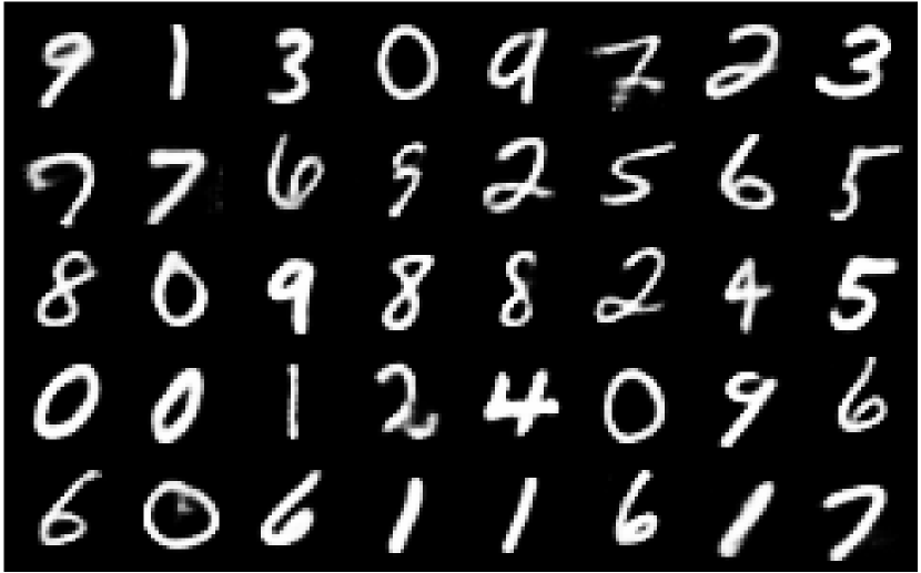
(a) MNIST (Bernoulli)

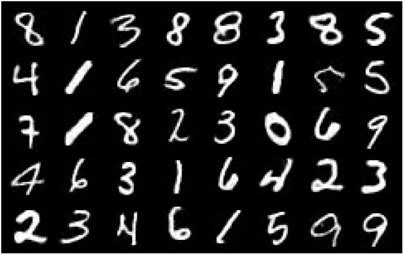
(b) MNIST

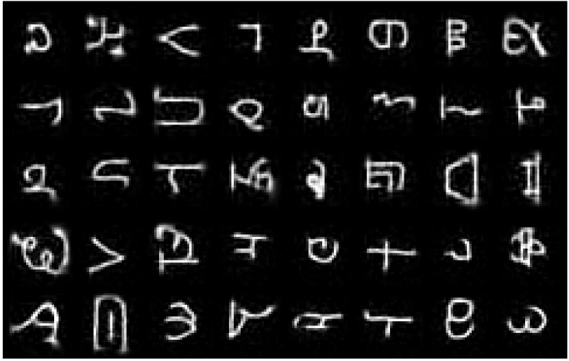
(c) Omniglot

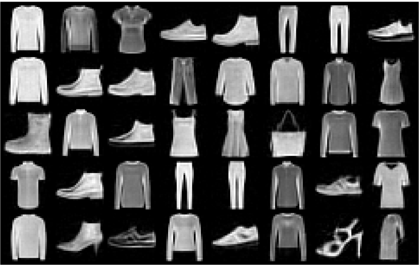
(d) Fashion MNIST

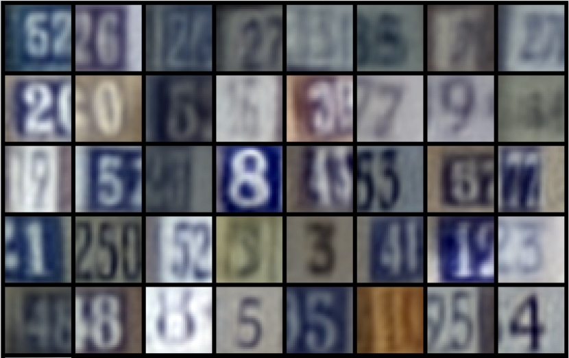
(e) SVHN

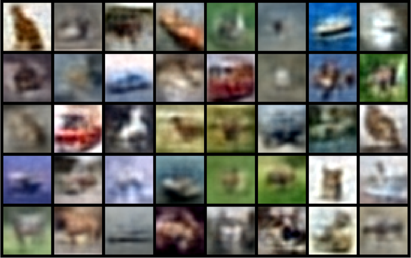
(f) CIFAR10

Figure 1: Examples of sample reconstructions by VLAE. Gaussian output distribution is used unless otherwise stated.

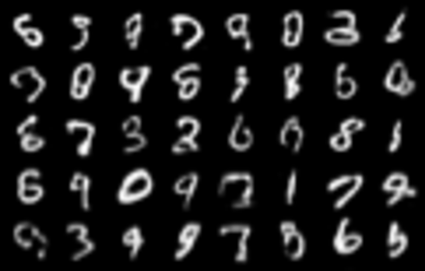
(a) MNIST (Bernoulli)

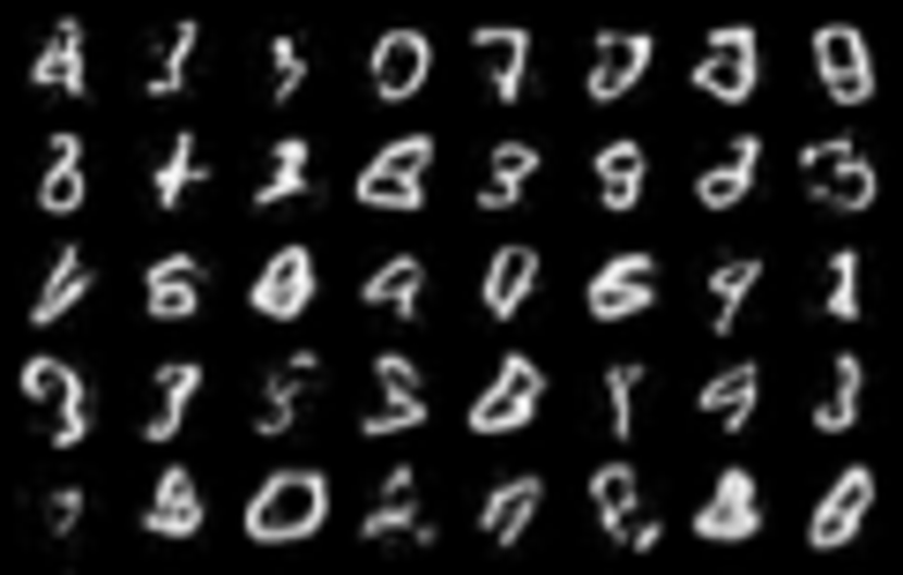
(b) MNIST

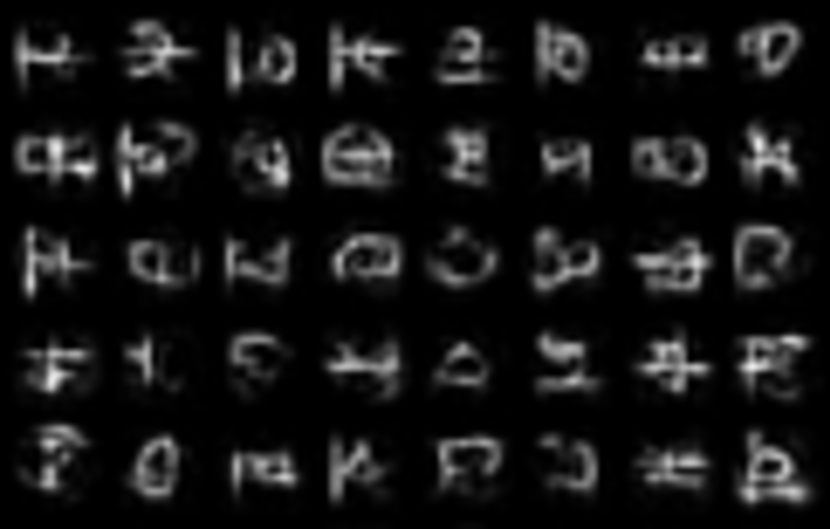
(c) Omniglot

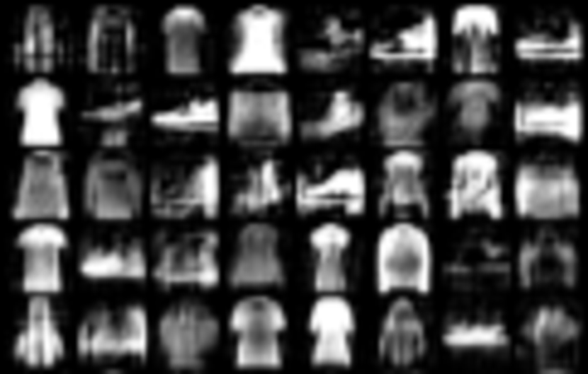
(d) Fashion MNIST

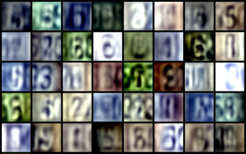
(e) SVHN

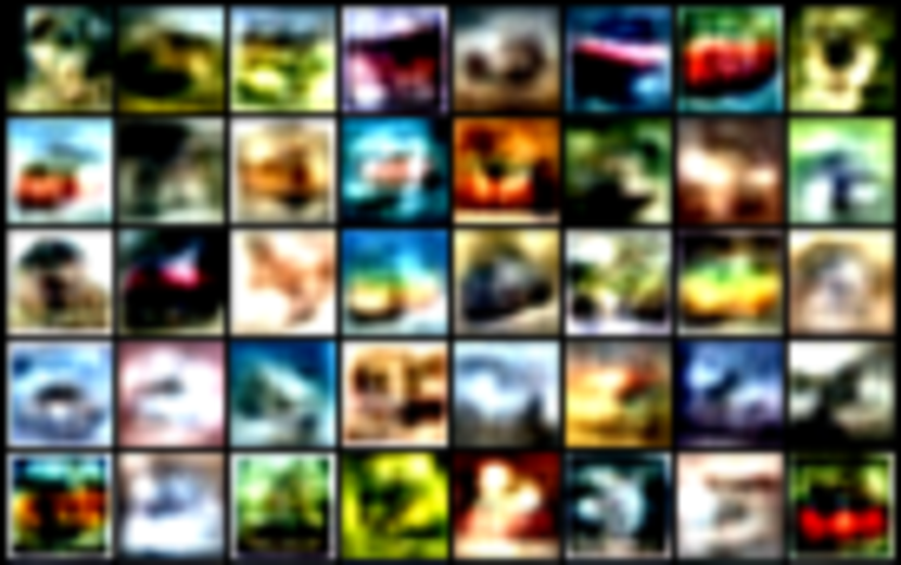
(f) CIFAR10

Figure 2: Examples of output samples generated by VLAE. Gaussian output distribution is used unless otherwise stated.

1 Image Samples

Figure 1 and 2 illustrates examples of reconstruction and generation samples made by the VLAE on MNIST (lecun98), Fashion MNIST (xiao17), Omniglot (lake13), SVHN (netzer11) and CIFAR 10 (krizhevsky09). Overall, the reconstructions are sharp but generated samples tend to be blurry, especially when the data is complex (e.g. CIFAR10). We expect using convolutional architectures to be helpful for improving image generation qualities.

2 Experimental Details

We optimize using ADAM (kingma15) with learning rate 0.0005. Other parameters of the optimizer is set to default values. We experiment with $T=1,2,4,8$ where $T$ is the number of iterative updates for VLAE and SA-VAE, or the number of flow transformations for VAE+HF. We set the batch size to 128. All models are trained up to 2000 epochs at maximum and evaluated using the checkpoint that gives the best validation performance.

We set $\alpha_{t}=0.5/(t+1)$ as decay for the VLAE update. For SA-VAE, the variational parameter $\bm{\mathbf{\lambda}}_{t}$ is updated $T$ times using SGD: $\bm{\mathbf{\lambda}}_{t+1}=\bm{\mathbf{\lambda}}_{t}+\alpha\frac{\partial}{\partial\bm{\mathbf{\phi}}}\mathcal{L}_{\bm{\mathbf{\theta}}}(\bm{\mathbf{x}};\bm{\mathbf{\lambda}}_{t})$ with $\alpha=0.0005$. The value of $\alpha$ is determined using a grid search among {1.0, 0.1, 0.001, 0.0005, 0.0001} on the small network. We estimate the gradient using a single sample of $\bm{\mathbf{z}}$ and apply the gradient norm clipping to avoid divergence of SA-VAE.

In our experiments, we find that the bigger models are susceptible to the parameter initialization, and their latent variables are prone to collapse if not properly initialized. We also observe VLAE and VAE+IAF are relatively robust to hyperparameter settings compared to other models. In order to prevent latent variable collapse, we use He’s initialization (he15) to preserve variance of backward propagation with gain of $2^{1/3}$ to account for the network structure that consists of two ReLU layer and one linear layer. In this way, the variance of gradients is preserved in initial phase of training. Furthermore, the data is mean-normalized and scaled so that the reconstruction loss at initial state is approximately $1$. These changes successfully prevent latent variable collapse and significantly improve overall performance of the models.

This finding hints that it is crucial to preserve gradient variance throughout the networks. Note that the gradient signal to the encoder comes from two sources: (1) KL divergence term $D_{KL}(q_{\bm{\mathbf{\phi}}}(\bm{\mathbf{z}}|\bm{\mathbf{x}})||p(\bm{\mathbf{z}}))$ (2) Reconstruction term $\mathbb{E}_{q_{\bm{\mathbf{\phi}}}(\bm{\mathbf{z}}|\bm{\mathbf{x}})}[\ln p_{\bm{\mathbf{\theta}}}(\bm{\mathbf{x}}|\bm{\mathbf{z}})]$. While the gradient from the KL divergence term is directly fed into the encoder, the gradient from the reconstruction term - which is essential for preventing the latent variable collapse - have to propagate backwards through the decoder to reach the encoder. We hypothesize that if the networks are not initialized properly, the reconstruction gradient is overwhelmed by the KL divergence gradient which drives the approximate posterior $q_{\bm{\mathbf{\phi}}}(\bm{\mathbf{z}}|\bm{\mathbf{x}})$ to collapse to the prior $p(\bm{\mathbf{z}})$ in the initial stage of training.

3 Conjugate Gradient Method

To measure the performance of the Conjugate Gradient (CG) method as an alternative to the update equations of the main draft, we implement the VLAE+CG model where the mode update equation is replaced with the CG ascent step. We use nonlinear Conjugate Gradient of Polak-Ribiére method. For more details on nonlinear Conjugate Gradient methods, we refer readers to (shewchuk1994introduction; dai2010nonlinear). With $T=4$, we find that VLAE+CG yields about 25% speed-up compared to the VLAE with minor performance loss ($\sim$ 1%) on MNIST.