The Bounded Gaussian Mechanism
for Differential Privacy

Abstract.

The Gaussian mechanism is one differential privacy mechanism commonly used to protect numerical data. However, it may be ill-suited to some applications because it has unbounded support and thus can produce invalid numerical answers to queries, such as negative ages or human heights in the tens of meters. One can project such private values onto valid ranges of data, though such projections lead to the accumulation of private query responses at the boundaries of such ranges, thereby harming accuracy. Motivated by the need for both privacy and accuracy over bounded domains, we present a bounded Gaussian mechanism for differential privacy, which has support only on a given region. We present both univariate and multivariate versions of this mechanism and illustrate a significant reduction in variance relative to comparable existing work.

Introduction

As many engineering applications have become increasingly reliant on user data, data privacy has become a concern that data aggregators and curators must take into consideration. In numerous applications, such as healthcare Yang et al. (2018), energy systems Asghar et al. (2017), transportation systems Zhang and Zhu (2018) and Internet of Things (IoT) Medaglia and Serbanati (2010), the data gathered to support system operation often contains sensitive individual information. Differential privacy Dwork and Roth (2014) has emerged as a standard privacy framework that can be used in such applications to protect sensitive data while allowing privatized data to remain useful. Differential privacy is a statistical notion of privacy that provides privacy guarantees by adding carefully calibrated noise to sensitive data or functions of sensitive data. Its key features include: (i) it is robust to side information, in that any additional knowledge about data-producing entities does not weaken their privacy by much Kasiviswanathan and Smith (2014), and (ii) it is immune to post-processing, in that any transformation of private data stays private Dwork and Roth (2014).

Well-known mechanisms for the enforcement of differential privacy include the Laplace mechanism Dwork et al. (2006), the Gaussian mechanism Dwork and Roth (2014), and the exponential mechanism McSherry and Talwar (2007); McSherry (2009). Other mechanisms have been developed for specific applications, in some cases by building upon or modifying these well-known mechanisms. A representative sample includes the Dirichlet mechanism on the unit simplex Gohari et al. (2021), mechanisms for sensitive words of symbolic data Chen et al. (2022), the matrix-variate Gaussian mechanism for matrix-valued queries Chanyaswad et al. (2018), and the XOR mechanism for binary-valued data Ji et al. (2021). As the use of differential privacy has grown, these and other mechanisms have been needed to respond to privacy needs in settings with constraints on allowable data.

The Gaussian mechanism has been used for some classes of numerical data, although it may also require modifications for some types of sensitive data because the Gaussian mechanism adds unbounded noise. For example, the Gaussian mechanism may generate negative values for data such as ages, salaries, and weights, and such negative values are not meaningful in these contexts. One attempt to solve this problem is through projecting out-of-domain results back to the closest value in the given domain. Although this procedure does not weaken differential privacy because it is only post-processing on private data, it has been observed to lead to low accuracy in applications Holohan et al. (2018) and thus is undesirable. Nonetheless, the Gaussian mechanism has been used in numerous applications, including deep learning Abadi et al. (2016), Yu et al. (2019), convex optimization Bassily et al. (2014), filtering and estimation problems Le Ny and Pappas (2014) and cloud control Hale and Egerstedt (2018), all of which can use data that is inherently bounded in some way.

On the other hand, compared to the Laplace mechanism, which is another popular privacy mechanism designed for numerical data, the Gaussian mechanism is able to use lower-variance noise to provide the same privacy level for high-dimensional data. This is because the variance of privacy noise is an increasing function of the sensitivity of a given query, and the Gaussian mechanism allows the use of the $L_{2}$ sensitivity which, in applications like federated learning Wei et al. (2020) and deep learning Abadi et al. (2016), is much lower than the $L_{1}$ sensitivity used in Laplace mechanism.

Therefore, in this paper we develop a new type of Gaussian mechanism that accounts for the boundedness of semantically valid data in a given application. In the univariate case we consider data confined to a closed interval, and in the multivariate case we consider data confined to a product of closed intervals. For both cases we show that the bounded Gaussian mechanism provides $\epsilon$-differential privacy, rather than $(\epsilon,\delta)$-differential privacy as is provided by the ordinary Gaussian mechanism. We also present algorithms for finding the minimum variance necessary to enforce $\epsilon$-differential privacy using the bounded Gaussian mechanism. The mechanisms we develop do not rely on projections and thus avoid the harms to accuracy that can accompany projection-based approaches.

Besides, Balle and Wang (2018) point out that the original Gaussian mechanism’s variance bound is far from tight when the privacy parameter $\epsilon$ approaches either $0$ or $\infty$. This is because the original Gaussian mechanism calibrates noise with a worst-case bound which is only tight for a small range of $\epsilon$. In this work, we present bounded mechanisms that address this limitation by leveraging the boundedness of the domains we consider. This boundedness excludes the tail of each Gaussian distribution from our analysis and allows for the development of tight bounds on the variance of noise required for all $\epsilon$.

Related work in Holohan et al. (2018) developed a bounded Laplace mechanism, and in this work we bring the ability to bound private data to the Gaussian mechanism. Developments in Liu (2019) include a generalized Gaussian mechanism with bounded support, and we show in Section 4 that the mechanism developed in this paper requires significantly lower variance of noise to attain differential privacy and thus provides improved accuracy.

Notation Let $\mathbb{N}$ denote the set of all positive integers and let $I$ denote the identity matrix. We use non-bold letters to denote scalars, e.g., $a\in\mathbb{R}$, and we use bold letters denote vectors, e.g., $\mathbf{b}\in\mathbb{R}^{n}$. All intervals of the form $[a,b]$ are assumed to have $a<b$. For $\mathbf{a},\mathbf{b}\in\mathbb{R}^{m}$ we define $[\mathbf{a},\mathbf{b}]=[a_{1},b_{1}]\times[a_{2},b_{2}]\times\cdots\times[a_{m},b_{m}]$. We also use the function

$$\text{erf}(z)=\frac{2}{\sqrt{\pi}}\int_{0}^{z}e^{-t^{2}}dt.$$

1. Preliminaries and Problem Statement

This section gives background on differential privacy and problem statements that are the focus of the remainder of the paper.

1.1. Differential Privacy Background

Differential privacy is enforced by a mechanism, which is a randomized map. We let $S$ denote the space of sensitive data of interest. For nearby pieces of sensitive data, a mechanism must produce outputs that are approximately distinguishable. The definition of “nearby” is given by an adjacency relation.

[Adjacency] Fix $k\in\mathbb{N}$. Two databases $d,d^{\prime}\in S^{n}$ are adjacent if they differ in $k$ rows.

For numerical queries $Q:S^{n}\rightarrow\mathbb{R}^{m}$, $m\in\mathbb{N}$, the sensitivity of a query $Q$, denoted $\Delta Q$, is used to calibrate the variance of privacy noise used to implement privacy. Throughout this paper we will use the $\ell_{2}$-sensitivity. [$\ell_{2}$-Sensitivity] The $\ell_{2}$-sensitivity of a query $Q:S^{n}\rightarrow\mathbb{R}^{m}$ is

$$\Delta Q:=\max_{\text{adjacent }d,d^{\prime}}||Q(d)-Q(d^{\prime})||_{2}.$$

The $\ell_{2}$ sensitivity captures the largest magnitude by which the outputs of $Q$ can change across two adjacent input databases. We next introduce the definition of differential privacy itself.

[Differential Privacy] Fix a probability space $(\Omega,\mathfrak{F},\mathbb{P})$, an adjacency parameter $k\in\mathbb{N}$, a privacy parameter $\epsilon>0$, and a query $Q:S^{n}\rightarrow\mathbb{R}^{m}$. A mechanism $M:\Omega\times S^{n}\to\mathbb{R}^{m}$ is $(\epsilon,\delta)$-differentially private if for all measurable sets $A\subseteq\mathbb{R}^{m}$ and for all adjacent databases $d,d^{\prime}\in S^{n}$ it satisfies $\mathbb{P}\big{[}M(Q(d))\in A\big{]}\leq e^{\epsilon}\mathbb{P}\big{[}M(Q(d^{\prime}))\in A\big{]}+\delta$.

The privacy parameter $\epsilon$ sets the strength of privacy protections, and a smaller $\epsilon$ implies stronger privacy. The parameter $\delta$ can be interpreted as a relaxation parameter, in the sense that it is the probability that $\epsilon$-differential privacy fails to hold Beimel et al. (2013) (though it may hold with a different value of $\epsilon$). If $\delta=0$, then a mechanism is said to be $\epsilon$-differentially private.

In the literature, $\epsilon$ has ranged from $0.01$ to $10$ (Hsu et al. (2014)). A differential privacy mechanism guarantees that the randomized outputs of two adjacent databases will be made approximately indistinguishable to any recipient of their privatized forms, including any eavesdroppers. One widely used differential privacy mechanism is the Gaussian mechanism. The standard Gaussian mechanism is given by the following theorem:

Theorem 1 (Standard Gaussian Mechanism).

Let $\epsilon\in(0,1)$ and $\delta\in(0,1]$ be given. Fix an adjacency parameter $k\in\mathbb{N}$. For $c^{2}>2\ln{(1.25/\delta)}$ and a query $Q$ of the database $d$, the Gaussian mechanism $M_{G}(Q(d))=Q(d)+\eta$, $\eta\sim\mathcal{N}(\mathbf{0},\sigma^{2}I)$ with parameter $\sigma^{2}\geq c\Delta Q/\epsilon$ is $(\epsilon,\delta)$-differentially private.

As discussed in the introduction, the Gaussian mechanism has been favored over the Laplace mechanism in several applications, including deep learning, empirical risk minimization, and various problems in control theory and optimization. Simultaneously, these applications may have bounds on the data they use, such as bounds on training data for a learning algorithm or bounds on states in a control system, though the Gaussian mechanism has infinite support and hence produces unbounded private outputs.

1.2. Problem Statement

In this work we seek a Gaussian mechanism that respects given bounds on data, and we formalize the development of this mechanism in the next two problem statements.

Problem 2 (Univariate bounded Gaussian mechanism).

Given a query $Q:S^{n}\rightarrow D$, where $D=[a,b]\subset\mathbb{R}$ ($a<b$, both finite) is a constrained domain, and a privacy parameter $\epsilon>0$, develop a mechanism $M_{B}:\Omega\times S^{n}\to D$ that is an $\epsilon$-differentially private approximation of $Q$ and generates outputs in $D$ with probability $1$.

Problem 3 (Multivariate bounded Gaussian mechanism).

Given a query $Q:S^{n}\rightarrow D$, where $D=[\mathbf{a},\mathbf{b}]\subset\mathbb{R}^{m}$ ($a_{i}<b_{i}$, both finite for all $i$) is a constrained domain, and a privacy parameter $\epsilon>0$, develop a mechanism $M_{B}:\Omega\times S^{n}\to D$ that is an $\epsilon$-differentially private approximation of $Q$ and generates outputs in $D$ with probability $1$.

We solve Problem 2 in Section 2, and we solve Problem 3 in Section 3.

2. Univariate Bounded Gaussian mechanism

In this section, we develop the bounded Gaussian mechanism for a bounded domain $D=[a,b]\subset\mathbb{R}$. We now give a formal statement of the univariate bounded Gaussian mechanism, and this will be the focus of the rest of this section:

[Univariate Bounded Gaussian Mechanism] Fix $\sigma>0$. Let a query $Q:S^{n}\to D$ be given where $D=[a,b]\subset\mathbb{R}$, and suppose that $d\in S^{n}$ generates the output $Q(d)=s\in D$. Then the univariate bounded Gaussian mechanism $M_{B}:\Omega\times S^{n}\to D$ is given by the probability density function

$$p_{B}(x)=\begin{cases}\frac{1}{\sigma}\frac{\phi\left(\frac{x-s}{\sigma}\right)}{\Phi\left(\frac{b-s}{\sigma}\right)-\Phi\left(\frac{a-s}{\sigma}\right)}&\text{if }x\in D,\\ 0&\text{otherwise,}\end{cases}$$ (1)

where

$$\phi(x)=\frac{1}{\sqrt{2\pi}}\exp\left(-\frac{1}{2}x^{2}\right),$$

$$\Phi(x)=\frac{1}{2}\left(1+\text{erf}(x/\sqrt{2})\right).$$

Since $Q(d)=s$, the density function $p_{B}(x)$ is not the same for each database, and data-dependent noise is known to be problematic in general for differential privacy Nissim et al. (2007). Therefore using the parameters of the standard Gaussian mechanism is no longer guaranteed to satisfy differential privacy for the bounded Gaussian mechanism. We next provide the parameters required for the bounded Gaussian mechanism to provide differential privacy by first introducing some preliminary results.

2.1. Preliminary Results

Lemma 4.

Let $\sigma>0$ be given. For a database $d\in S^{n}$ and a query $Q$ with $Q(d)=s\in D$ and $D=[a,b]\subset\mathbb{R}$, let

$$C(s,\sigma)=\frac{1}{\Phi\left(\frac{b-s}{\sigma}\right)-\Phi\left(\frac{a-s}{\sigma}\right)}.$$ (2)

Let $d^{\prime}\in S^{n}$ be adjacent to $d$ in the sense of Definition 1.1, and suppose that $Q(d^{\prime})=s^{\prime}\in D$. Then we have

$$\max_{s,s^{\prime}}\frac{C(s,\sigma)}{C(s^{\prime},\sigma)}=\frac{C(a,\sigma)}{C(a+c,\sigma)},$$

where $c=|s^{\prime}-s|\leq\Delta Q$.

Proof 2.1.

See Appendix A.

This leads to the following lemma.

Lemma 5.

Let $C(s,\sigma)$ be given in Equation (2). Given two adjacent databases $d\in S^{n}$ and $d^{\prime}\in S^{n}$ and a query $Q:S^{n}\rightarrow D$, suppose that $Q(d)=s$ and $Q(d^{\prime})=s^{\prime}$ such that $s^{\prime}=s+c$ and by the definition of adjacency we have $|c|\leq\Delta Q$. Then

$$\max_{c}\frac{C(a,\sigma)}{C(a+c,\sigma)}=:\Delta C(\sigma)=\begin{cases}\frac{C(a,\sigma)}{C(a+\Delta Q,\sigma)}&\text{if }\Delta Q\leq\frac{b-a}{2},\\[5.0pt] \frac{C(a,\sigma)}{C\left(\frac{b+a}{2},\sigma\right)}&\textnormal{otherwise.}\end{cases}$$

Proof 2.2.

See Appendix B.

2.2. Main Result on the Univariate Bounded Gaussian Mechanism

We now proceed to the main result of this section, which bounds the variance required for the bounded Gaussian mechanism to provide $\epsilon$-differential privacy.

Theorem 6.

Let $\epsilon>0$ and let a query $Q:S^{n}\to D$ be given. Suppose $d\in S^{n}$ generates the output $Q(d)=s\in D$ and $D=[a,b]\subset\mathbb{R}$. Then the Univariate Bounded Gaussian mechanism $M_{B}$ provides $\epsilon$-differential privacy if

$$\sigma^{2}\geq\frac{\left[(b-a)+\frac{\Delta Q}{2}\right]\Delta Q}{\epsilon-\ln(\Delta C(\sigma))}.$$ (3)

Proof 2.3.

See Appendix C.

We observe that in Equation (3) the privacy noise variance $\sigma$ appears on both sides of the equation. Given a value of $\epsilon>0$, it is desirable to use the smallest $\sigma$ as this corresponds to using the smallest variance of privacy noise for a given privacy level. To do so, in the next section, we form a zero finding problem to find the minimum $\sigma$ that satisfies Equation (3).

2.3. Calculating $\sigma$

Let $\sigma^{*}$ be the smallest admissible value of $\sigma$. The calculation of $\sigma^{*}$ can be formulated as a zero finding problem, where we require

$$f(\sigma^{*})=(\sigma^{*})^{2}-\frac{\left[(b-a)+\frac{\Delta Q}{2}\right]\Delta Q}{\epsilon-\ln(\Delta C(\sigma^{*}))}=0.$$ (4)

We now present some technical lemmas concerning the function $f$ with respect to a point

$$\sigma_{0}=\sqrt{\frac{\left[(b-a)+\frac{\Delta Q}{2}\right]\Delta Q}{\epsilon}}.$$ (5)

Lemma 7.

For any $\epsilon>0$, we have $\epsilon-\ln(\Delta C(\sigma_{0}))>0$.

Proof 2.4.

See Appendix D.

Lemma 8.

For all $\sigma\in(0,\infty)$, we have $\ln(\Delta C(\sigma))>0$.

Proof 2.5.

See Appendix E.

Next, Lemma 9 shows the value of $f(\sigma_{0})$ and Lemma 10 shows $f$ is a monotonically increasing function on $[\sigma_{0},\infty)$.

Lemma 9.

For the point $\sigma_{0}=\sqrt{\frac{\left[(b-a)+\frac{\Delta Q}{2}\right]\Delta Q}{\epsilon}}$, we have $f(\sigma_{0})<0$.

Proof 2.6.

By plugging in $\sigma_{0}$ we have

$$f(\sigma_{0})=\frac{\left[(b-a)+\frac{\Delta Q}{2}\right]\Delta Q}{\epsilon}-\frac{\left[(b-a)+\frac{\Delta Q}{2}\right]\Delta Q}{\epsilon-\ln(\Delta C(\sigma_{0}))}.$$

By Lemma 7 and Lemma 8 we have $\epsilon>\epsilon-\ln(\Delta C(\sigma_{0}))>0$. Therefore $f(\sigma_{0})<0$.

Lemma 10.

For any $\sigma\in[\sigma_{0},\infty)$, we have $f^{\prime}(\sigma)>0$.

Proof 2.7.

See Appendix F.

By combining Lemma 9 and Lemma 10, we can use Algorithm 1 in Holohan et al. (2018), given below as Algorithm 1, to find the exact fixed point of $f$, which in our case is $\sigma^{*}$.

Input : Function $f$ given in Equation (4), initial condition for privacy noise variance $\sigma_{0}$ given in Equation (5)

Output : Optimal privacy parameter $(\sigma^{*})^{2}$

left$=\sigma_{0}^{2}$;

right$=\frac{\left[(b-a)+\frac{\Delta Q}{2}\right]\Delta Q}{\epsilon-\ln(\Delta C(\sigma_{0}))}$;

intervalSize$=($left$+$right$)/2$;

while intervalSize$>$right$-$left do

       intervalSize $=$ right $-$ left;

       $(\sigma^{*})^{2}=\frac{\text{left}+\text{right}}{2}$;

       if $\frac{\left[(b-a)+\frac{\Delta Q}{2}\right]\Delta Q}{\epsilon-\ln(\Delta C(\sigma^{*}))}\geq(\sigma^{*})^{2}$ then

             left $=(\sigma^{*})^{2}$;

            

       end if

      if $\frac{\left[(b-a)+\frac{\Delta Q}{2}\right]\Delta Q}{\epsilon-\ln(\Delta C(\sigma^{*}))}\leq(\sigma^{*})^{2}$ then

             right $=(\sigma^{*})^{2}$ ;

            

       end if

      

end while

return $(\sigma^{*})^{2}$

Algorithm 1 A Zero Finding Algorithm

The output of Algorithm 1 can be used in Definition 2 to form the univariate bounded Gaussian mechanism, and Theorem 6 shows that doing so provides $\epsilon$-differential privacy. We next present an analogous mechanism for multi-variate query responses.

3. Multivariate Bounded Gaussian mechanism

We begin by formally defining the multivariate bounded Gaussian mechanism, and it will be the focus of the remainder of this section.

[Multivariate Bounded Gaussian Mechanism] Fix $\sigma_{m}>0$. Let a query $Q:S^{n}\to D$ be given, where $D=[\mathbf{a},\mathbf{b}]\subset\mathbb{R}^{m}$. For a database $d\in S^{n}$ and its output $Q(d)=\mathbf{s}\in D$, the multivariate bounded Gaussian mechanism $M_{B}^{m}:\Omega\times\mathbb{R}^{n}\to D$ is given by the probability density function

$$p_{B}(\mathbf{x})=\begin{cases}\frac{\exp{\left(-\frac{1}{2}(\mathbf{x}-\mathbf{s})^{T}\Sigma^{-1}(\mathbf{x}-\mathbf{s})\right)}}{\int_{\mathbf{a}}^{\mathbf{b}}\exp{\left(-\frac{1}{2}(\mathbf{x}-\mathbf{s})^{T}\Sigma^{-1}(\mathbf{x}-\mathbf{s})\right)}d\mathbf{x}}&\text{if }\mathbf{x}\in D,\\[5.0pt] 0&\text{otherwise,}\end{cases}$$ (6)

where $\Sigma=\sigma_{m}^{2}I\in\mathbb{R}^{m\times m}$.

Before introducing the this mechanism’s differential privacy guarantee we first require some preliminary results.

3.1. Preliminary Results

Lemma 11.

Fix $\sigma_{m}>0$. For a database $d\in S^{n}$ and a query $Q(d)=\mathbf{s}\in D$ and $D=[\mathbf{a},\mathbf{b}]\subset\mathbb{R}^{m}$, let

$$C_{m}(\mathbf{s},\sigma_{m})=\frac{1}{\int_{\mathbf{a}}^{\mathbf{b}}\exp{\left(-\frac{1}{2}(\mathbf{x}-\mathbf{s})^{T}\Sigma^{-1}(\mathbf{x}-\mathbf{s})\right)}d\mathbf{x}}.$$ (7)

Let an adjacent database $d^{\prime}\in S^{m}$ satisfy $Q(d^{\prime})=\mathbf{s}^{\prime}\in D$. Then we have

$$\max_{\mathbf{s},\mathbf{s}^{\prime}}\frac{C_{m}(\mathbf{s},\sigma_{m})}{C_{m}(\mathbf{s}^{\prime},\sigma_{m})}=\frac{C_{m}(\mathbf{a},\sigma_{m})}{C_{m}(\mathbf{a}+\mathbf{c},\sigma_{m})},$$

where $c_{i}=|s_{i}-s_{i}^{\prime}|$ for the $i^{th}$ element of $\mathbf{c}\in\mathbb{R}^{m}$ and $||\mathbf{c}||_{2}\leq\Delta Q$.

Proof 3.1.

See Appendix G.

Now we define $\Delta C_{m}(\sigma_{m},\mathbf{c}^{*})$, where

$$\frac{C_{m}(\mathbf{a},\sigma_{m})}{C_{m}(\mathbf{a}+\mathbf{c},\sigma_{m})}\leq\frac{C_{m}(\mathbf{a},\sigma_{m})}{C_{m}(\mathbf{a}+\mathbf{c}^{*},\sigma_{m})}=:\Delta C_{m}(\sigma_{m},\mathbf{c}^{*}),$$

where $\mathbf{c}^{*}\in\mathbb{R}^{m}$ is the optimal value of $\mathbf{c}=(c_{1},\dots,c_{m})^{T}$ in the following optimization problem:

$$\max_{\mathbf{c}\in\mathbb{R}^{m}}\,\,\, \Delta C_{m}(\sigma_{m},\mathbf{c})$$ (8)

subject to $$0\leq c_{i}\leq b_{i}-a_{i}\text{ for each }i$$

$$||\mathbf{c}||_{2}\leq\Delta Q.$$

Remark 12.

The optimization problem in (8) is a concave maximization problem. In general, the value of $c^{*}$ does not have a closed form, but it can be efficiently computed numerically using standard optimization software such as CVX or CasADi.

3.2. Main Results

We now proceed to the main result of this section, which bounds the variance required for the multivariate bounded Gaussian mechanism to provide $\epsilon$-differential privacy.

Theorem 13.

Let $\epsilon>0$ and a query $Q:S^{n}\to D$ be given. For a database $d\in S^{n}$ and its output $Q(d)=\mathbf{s}\in D$, where $D=[\mathbf{a},\mathbf{b}]\subset\mathbb{R}^{n}$, the multivariate bounded Gaussian mechanism $M_{B}$ provides $\epsilon$-differential privacy if

$$\sigma_{m}^{2}\geq\frac{\left[||\mathbf{b-a}||_{2}+\frac{\Delta Q}{2}\right]\Delta Q}{\epsilon-\ln(\Delta C_{m}(\sigma_{m},\mathbf{c}^{*}))}.$$ (9)

Proof 3.2.

See Appendix H.

As with the univariate bounded Gaussian mechanism, we see that $\sigma_{m}$ appears on both sides of (9). Hence, we will use numerical methods to compute it.

3.3. Calculating $\sigma_{m}$

We will follow similar steps to those in Section 2.3. Let $\sigma_{m}^{*}$ be the minimal admissible value of $\sigma_{m}$ that satisfies (9). Then for $D\subset\mathbb{R}^{m}$ we have

$$f_{m}(\sigma_{m}^{*})=(\sigma_{m}^{*})^{2}-\frac{\left[||\mathbf{b}-\mathbf{a}||_{2}+\frac{\Delta Q}{2}\right]\Delta Q}{\epsilon-\ln(\Delta C_{m}(\sigma_{m}^{*},\mathbf{c}^{*}))}=0.$$ (10)

We now present some lemmas concerning the function $f_{n}$ with respect to the point

$$\sigma_{m,0}=\sqrt{\frac{\left[||\mathbf{b}-\mathbf{a}||_{2}+\frac{\Delta Q}{2}\right]\Delta Q}{\epsilon}}.$$ (11)

Lemma 14.

For any $\epsilon>0$, we have $\epsilon-\ln(\Delta C_{m}(\sigma_{m,0},\mathbf{c}^{*}))>0$, where $\mathbf{c}^{*}$ is defined in Equation (8).

Proof 3.3.

See Appendix I.

Lemma 15.

For $\sigma_{m,0}=\sqrt{\frac{\left[||\mathbf{b}-\mathbf{a}||_{2}+\frac{\Delta Q}{2}\right]\Delta Q}{\epsilon}}$, we have $\ln(\Delta C_{m}(\sigma_{m,0},\mathbf{c}^{*}))>0$.

Proof 3.4.

See Appendix J.

Lemma 16.

For a point $\sigma_{m,0}=\sqrt{\frac{\left[||\mathbf{b}-\mathbf{a}||_{2}+\frac{\Delta Q}{2}\right]\Delta Q}{\epsilon}}$, we have $f_{m}(\sigma_{m,0})<0$.

Proof 3.5.

By plugging in $\sigma_{m,0}$ we have

$$f_{m}(\sigma_{m,0})=\frac{\left[||\mathbf{b}-\mathbf{a}||_{2}+\frac{\Delta Q}{2}\right]\Delta Q}{\epsilon}-\frac{\left[||\mathbf{b}-\mathbf{a}||_{2}+\frac{\Delta Q}{2}\right]\Delta Q}{\epsilon-\ln(\Delta C_{m}(\sigma_{m,0},\mathbf{c}^{*}))}.$$

With Lemma 14 and Lemma 15 we have $\epsilon>\epsilon-\ln(\Delta C_{m}(\sigma_{m,0},\mathbf{c}^{*}))>0$. Therefore $f_{m}(\sigma_{m,0})<0$.

Lemma 17.

For any $\sigma_{m}\in[\sigma_{m,0},\infty)$, we have $f_{m}^{\prime}(\sigma)>0$.

Proof 3.6.

See Appendix K.

By combining Lemma 16 and Lemma 17 we can use Algorithm 1 in Holohan et al. (2018) to find the exact fixed point of $f_{m}$, namely $\sigma_{m}^{*}$, which is shown in Algorithm 2. The output of Algorithm 2 can be combined with the mechanism in Definition 3, and Theorem 13 shows that this combination gives $\epsilon$-differential privacy for multivariate queries.

Input : Function $f_{m}$ given in Equation (10), Initial privacy parameter $\sigma_{m,0}$ given in Equation (11).

Output : Optimal privacy parameter $(\sigma_{m}^{*})^{2}$.

left$=\sigma_{m,0}^{2}$;

Compute $c^{*}$ from the optimization problem in (8);

rignt$=\frac{\left[||\mathbf{b-a}||_{2}+\frac{\Delta Q}{2}\right]\Delta Q}{\epsilon-\ln(\Delta C_{m}(\sigma_{m,0},\mathbf{c}^{*}))}$;

intervalSize$=($left$+$right$)*2$;

while intervalSize$>$right$-$left do

       intervalSize $=$ right $-$ left;

       $(\sigma_{m}^{*})^{2}=\frac{\text{left}+\text{right}}{2}$;

       Compute $c^{*}$ from the optimization problem in (8);

       if $\frac{\left[||b-a||_{2}+\frac{\Delta Q}{2}\right]\Delta Q}{\epsilon-\ln(\Delta C_{m}(\sigma_{m}^{*},\mathbf{c}^{*}))}\geq(\sigma_{m}^{*})^{2}$ then

             left $=(\sigma_{m}^{*})^{2}$;

            

       end if

      if $\frac{\left[||\mathbf{b-a}||+\frac{\Delta Q}{2}\right]\Delta Q}{\epsilon-\ln(\Delta C_{m}(\sigma_{m}^{*},\mathbf{c}^{*}))}\leq(\sigma_{m}^{*})^{2}$ then

             right $=(\sigma_{m}^{*})^{2}$;

            

       end if

      

end while

return $(\sigma_{m}^{*})^{2}$

Algorithm 2 A Zero Finding Algorithm for Multivariate Bounded Gaussian Mechanism

4. Numerical Results

This section presents simulation results. We consider queries of the properties of a graph. Specifically, the bounded data we consider is (i) the average degree in an undirected graph, and (ii) the second-smallest eigenvalue of the Laplacian of an undirected graph. This eigenvalue is also called the Fiedler value Fiedler (1973) of the graph. It is known that an undirected graph is connected if and only if its Fiedler value is positive Fiedler (1973), and the Fiedler value also sets the rate of convergence of various dynamical processes over graphs Mesbahi and Egerstedt (2010).

We let $G=(V,E)$ denote a connected, undirected graph on $10$ nodes. In this experiment we have a two-dimensional query $Q$ to compute (i) the algebraic connectivity, equal to the second smallest eigenvalue $\lambda_{2}$ of the Laplacian matrix of $G$, which satisfies $\lambda_{2}\in[0,10]$ here, and (ii) the degree of a fixed but arbitrary node $i$, denoted $N^{i}$, which satisfies $N^{i}\in[1,9]$ here. Therefore, for a graph $G$ we have $Q(G)=[\lambda_{2},N_{\text{out}}]^{T}\in D$, where $D=[\mathbf{a,b}]\subset\mathbf{R}^{2}$, with $\mathbf{a}=[0,1]^{T}$ and $\mathbf{b}=[10,9]^{T}$. For a fixed $k\in\mathbb{N}$, we say that two graphs are adjacent if they have the same node set but differ in $k$ edges. Let $\Delta Q_{\lambda_{2}}$ denote the sensitivity of $\lambda_{2}$, let $\Delta Q_{N^{i}}$ denote the sensitivity of node $i$’s degree, and let $\Delta Q=||(\Delta Q_{\lambda_{2}},\Delta Q_{N^{i}})^{T}||_{2}$ denote the sensitivity of the query $Q$. From (Chen et al., 2021, Lemma 1) we have $\Delta Q_{\lambda_{2}}=2k$ and $\Delta Q_{N^{i}}=k$. Thus, $\Delta Q=\sqrt{5}k$. In our simulations we set $k=2$. Table 1 gives some example variances computed for using the multivariate bounded Gaussian mechanism. In Figure 1, there is a general decrease in the variance of the bounded Gaussian mechanism as $\epsilon$ grows. This decrease agrees with intuition because a larger $\epsilon$ implies weaker privacy protection and thus the private output distribution has a higher peak on the true query answer.

We now compare the proposed mechanism with generalized Gaussian mechanism Liu (2019). Let $\sigma_{GG}^{2}$ be the variance of generalized Gaussian mechanism and $\sigma_{BG}^{2}$ be the bounded Gaussian mechanism. Then we define the Percent Reduction in variance as

$$\text{Percent Reduction}=\frac{\sigma_{GG}^{2}-\sigma_{BG}^{2}}{\sigma_{GG}^{2}}\times 100\%.$$

Both Figure 1 and Table 1 show that the bounded Gaussian mechanism always generates smaller variance, i.e., $\sigma_{BG}^{2}<\sigma_{GG}^{2}$ and the $\text{Percent Reduction}>0$ for all $\epsilon$. In other words, compared to the generalized Gaussian mechanism Liu (2019), the bounded Gaussian mechanism generates private outputs with less noise but with the same level of privacy protection.

$\epsilon$	Generalized Gaussian $\sigma_{GG}^{2}$	Bounded Gaussian $\sigma_{BG}^{2}$	Percent Reduction
0.1	1320.0	857.5	35.0%
0.5	264.0	170.3	35.5%
1.0	132.0	84.3	36.1%
1.5	88	55.8	36.6%
2.0	66	41.5	37.2%
2.5	52.8	32.9	37.7%
3.0	44	27.2	38.2%

Table 1. Some example values of $\sigma_{BG}$ with different values of $\epsilon$. The last column shows the percentage reduction in variance attained by using the bounded Gaussian mechanism we develop.

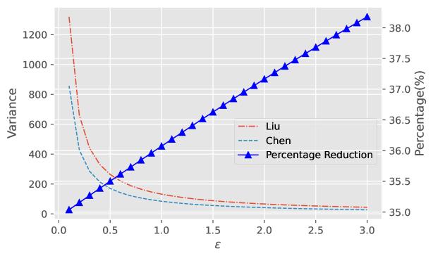
Figure 1. The variance comparison of proposed machanism and Liu’s mechanism from (Liu, 2019, Definition 5). With a larger $\epsilon$, which gives weaker privacy, the variance of bounded Gaussian mechanism decreases quickly and is always smaller than that of the generalized Gaussian mechanism. This means that the bounded Gaussian mechanisms require less noise and provide better accuracy while maintaining the same level of protection. In addition, the blue triangles ascent from left to right, indicating that the reduction in variance grows as $\epsilon$ grows.

5. Conclusion

This paper presented two differential privacy mechanisms, namely the univariate and multivariate bounded Gaussian mechanisms, for bounded domain queries of a database of sensitive data. Compared to the existing generalized Gaussian mechanism, the bounded Gaussian mechanisms we present generate private outputs with less noise and better accuracy for the same privacy level. Future work will apply this mechanism to real world applications, such as privately forecasting epidemic propagation, federated learning and optimization, and explore privacy and performance trade-off. Besides, future work will design a denoise post-processing procedure to generate more accurate private outputs.

Appendix A Proof of Lemma 4

By symmetry we can write $s^{\prime}=s+c$. We proceed in this proof by showing that $\frac{C(s,\sigma)}{C(s+c,\sigma)}$ is monotonically decreasing with respect to $s$. In other words, we show $\frac{\partial}{\partial s}\left(\frac{C(s,\sigma)}{C(s+c,\sigma)}\right)<0$. We first note that

$$\frac{C(s,\sigma)}{C(s+c,\sigma)} =\frac{\Phi\left(\frac{b-s-c}{\sigma}\right)-\Phi\left(\frac{a-s-c}{\sigma}\right)}{\Phi\left(\frac{b-s}{\sigma}\right)-\Phi\left(\frac{a-s}{\sigma}\right)}$$

$$=\frac{\int_{a}^{b}\phi\left(\frac{x-s-c}{\sigma}\right)dx}{\int_{a}^{b}\phi\left(\frac{x-s}{\sigma}\right)dx}$$

$$=\frac{\int_{a}^{b}\exp{\left(-\frac{1}{2}\left(\frac{x-s-c}{\sigma}\right)^{2}\right)}dx}{\int_{a}^{b}\exp{\left(-\frac{1}{2}\left(\frac{x-s}{\sigma}\right)^{2}\right)}dx}$$

$$=\frac{\int_{a-s}^{b-s}\exp{\left(-\frac{1}{2}\left(\frac{y-c}{\sigma}\right)^{2}\right)}dy}{\int_{a}^{b}\exp{\left(-\frac{1}{2}\left(\frac{x-s}{\sigma}\right)^{2}\right)}dx},$$ (12)

where $y=x-s$. We now introduce the Leibniz rule that we will use later in the proof.

Theorem 18 (Leibniz Integral Rule).

Let $g(x,t)$ be a function such that both $g(x,t)$ and its partial derivative $g_{x}(x,t)$ are continuous in $t$ and $x$ in some region of the $xt$-plane, including $f_{1}(x)\leq t\leq f_{2}(x)$, $x_{0}\leq x\leq x_{1}$. Also suppose that the functions $f_{1}(x)$ and $f_{2}(x)$ are both continuous and both have continuous derivatives for $x_{0}\leq x\leq x_{1}$. Then for $x_{0}\leq x\leq x_{1}$,

$$\frac{d}{dx}\left(\int_{f_{1}(x)}^{f_{2}(x)}g(x,t)dt\right)=g(x,f_{2}(x))\cdot\frac{d}{dx}f_{2}(x)-g(x,f_{1}(x))\cdot\frac{d}{dx}f_{1}(x)+\int_{f_{1}(x)}^{f_{2}(x)}\frac{d}{dx}g(x,t)dt.$$

Let $A(s)=\int_{a}^{b}\exp{\left(-\frac{1}{2}\left(\frac{x-s}{\sigma}\right)^{2}\right)}dx$. Using Theorem 18, the derivative of Equation (12) becomes

$$\frac{\partial}{\partial s}\left(\frac{C(s,\sigma)}{C(s+c,\sigma)}\right) =\frac{[\exp(-\frac{(a-c-s)^{2}}{2\sigma^{2}})-\exp(-\frac{(b-c-s)^{2}}{2\sigma^{2}})]A(s)}{A(s)^{2}}$$

$$\quad-\frac{[\exp(-\frac{(a-s)^{2}}{2\sigma^{2}})-\exp(-\frac{(b-s)^{2}}{2\sigma^{2}})]\int_{a}^{b}\exp(-\frac{(x-c-s)^{2}}{2\sigma^{2}})dx}{A(s)^{2}}.$$ (13)

We next introduce the mean value theorem of integrals.

Theorem 19 (Mean Value Theorem of Integrals).

For a continuous function $h:(a,b)\to\mathbb{R}$ and an integrable function $g$ that does not change sign on $[a,b]$, there exists $\alpha\in[a,b]$ such that

$$\int_{a}^{b}h(x)g(x)dx=h(\alpha)\int_{a}^{b}g(x)dx.$$

Using Theorem 19, we have

$$\int_{a}^{b}\exp\left(-\frac{(x-c-s)^{2}}{2\sigma^{2}}\right)dx =\int_{a}^{b}\exp\left(-\frac{1}{2\sigma^{2}}((x-s)^{2}-2(x-s)c+c^{2})\right)dx$$

$$=\exp\left(-\frac{c^{2}}{2\sigma^{2}}\right)\int_{a}^{b}\exp\left(-\frac{(x-s)^{2}}{2\sigma^{2}}\right)\exp\left(\frac{(x-s)c}{\sigma^{2}}\right)dx$$

$$=\exp\left(-\frac{c^{2}}{2\sigma^{2}}\right)\exp\left(\frac{(e-s)c}{\sigma^{2}}\right)A(s),$$ (14)

where $e\in[a,b]$. Then we plug Equation (14) into the Equation (13), and we have

$$\frac{\partial}{\partial s}\left(\frac{C(s,\sigma)}{C(s+c,\sigma)}\right)$$ (15)

$$=\exp\left(-\frac{c^{2}}{2\sigma^{2}}\right)\frac{[\exp(-\frac{(a-s)^{2}}{2\sigma^{2}})\exp(\frac{(a-s)c}{\sigma^{2}})-\exp(-\frac{(b-s)^{2}}{2\sigma^{2}})\exp(\frac{(b-s)c}{\sigma^{2}})]}{A(s)}$$

$$\quad-\exp\left(-\frac{c^{2}}{2\sigma^{2}}\right)\frac{[\exp(-\frac{(a-s)^{2}}{2\sigma^{2}})-\exp(-\frac{(b-s)^{2}}{2\sigma^{2}})]\exp(\frac{(e-s)c}{\sigma^{2}})}{A(s)}$$ (16)

$$=\frac{1}{A(s)}\exp\left(-\frac{c^{2}}{2\sigma^{2}}\right)\left[\exp\left(-\frac{(a-s)^{2}}{2\sigma^{2}}\right)\left(\exp\left(\frac{(a-s)c}{\sigma^{2}}\right)-\exp\left(\frac{(e-s)c}{\sigma^{2}}\right)\right)\right]$$

$$\quad+\frac{1}{A(s)}\exp\left(-\frac{c^{2}}{2\sigma^{2}}\right)\left[\exp\left(-\frac{(b-s)^{2}}{2\sigma^{2}}\right)\left(\exp\left(\frac{(e-s)c}{\sigma^{2}}\right)-\exp\left(\frac{(b-s)c}{\sigma^{2}}\right)\right)\right]$$ (17)

$$=\frac{1}{A(s)}\exp\left(-\frac{c^{2}}{2\sigma^{2}}\right)\left[\exp\left(-\frac{(a-s)^{2}}{2\sigma^{2}}\right)\cdot B(s,c)+\exp\left(-\frac{(b-s)^{2}}{2\sigma^{2}}\right)\cdot C(s,c)\right],$$ (18)

where

$$B(s,c)=\exp\left(\frac{(a-s)c}{\sigma^{2}}\right)-\exp\left(\frac{(e-s)c}{\sigma^{2}}\right)\leq 0,\quad\text{and equality is achieved if and only if }e=a,$$

$$C(s,c)=\exp\left(\frac{(e-s)c}{\sigma^{2}}\right)-\exp\left(\frac{(b-s)c}{\sigma^{2}}\right)\leq 0,\quad\text{if equality is achieved if and only if }e=b.$$

The Equation (16) comes by rewriting equation 13 using perfect square trinomial. The Equation (17) comes by rearranging these terms and factors out their common factors. The Equation (18) is just substituting $B(s,c)$ and $C(s,c)$.

Since $B(s,c)$ and $C(s,c)$ cannot be 0 at the same time, we have

$$\frac{\partial}{\partial s}\left(\frac{C(s,\sigma)}{C(s+c,\sigma)}\right)<0.$$

Since $s\in[a,b]$, we have

$$\max_{s}\frac{C(s,\sigma)}{C(s+c,\sigma)}=\frac{C(a,\sigma)}{C(a+c,\sigma)}.$$

Appendix B Proof of Lemma 5

We proceed this proof by forming a maximization problem and then use the Lagrangian multipliers method to solve it. By symmetry we assume $c>0$ and we have

$$\max_{c}\frac{C(a,\sigma)}{C(a+c,\sigma)}=\max_{c}\frac{\int_{a}^{b}\exp{\left(-\frac{1}{2}\left(\frac{x-a-c}{\sigma}\right)^{2}\right)}dx}{\int_{a}^{b}\exp{\left(-\frac{1}{2}\left(\frac{x-a}{\sigma}\right)^{2}\right)}dx}$$

$$\text{subject to}\quad c\in[0,\Delta Q].$$

Because this is a maximization problem, the Lagrangian function is formed as

$$\mathcal{L}(c,\lambda_{1},\lambda_{2})=\frac{C(a,\sigma)}{C(a+c,\sigma)}-\lambda_{1}(0-c)-\lambda_{2}(c-\Delta Q),$$

where $\lambda_{1}$,$\lambda_{2}\geq 0$. We then set $\frac{\partial\mathcal{L}(c,\lambda_{1},\lambda_{2})}{\partial c}=0$ and apply the Karush–Kuhn–Tucker (KKT) conditions to find

$$\frac{\partial}{\partial c}\left(\frac{C(a,\sigma)}{C(a+c,\sigma)}\right)+\lambda_{1}-\lambda_{2}=0$$ (19)

$$\lambda_{1}(0-c)=0$$ (20)

$$\lambda_{2}(c-\Delta Q)=0$$ (21)

The derivative term in Equation (19) can be further simplified as

$$\frac{\partial}{\partial c}\left(\frac{C(a,\sigma)}{C(a+c,\sigma)}\right) =\frac{1}{A(s)}\left(\frac{\partial}{\partial c}\int_{a}^{b}\exp{\left(-\frac{1}{2}\left(\frac{x-a-c}{\sigma}\right)^{2}\right)}dx\right)$$

$$=\frac{1}{A(s)}\left(\frac{\partial}{\partial c}\int_{a-c}^{b-c}\exp{\left(-\frac{1}{2}\left(\frac{z-a}{\sigma}\right)^{2}\right)}dz\right)$$

$$=\frac{1}{A(s)}\left(\exp\left(-\frac{(a-a-c)^{2}}{2\sigma^{2}}\right)-\exp\left(-\frac{(b-a-c)^{2}}{2\sigma^{2}}\right)\right)$$ (22)

$$=\frac{1}{A(s)}\left(\exp\left(-\frac{c^{2}}{2\sigma^{2}}\right)-\exp\left(-\frac{(c-(b-a))^{2}}{2\sigma^{2}}\right)\right),$$ (23)

where $z=x-c$. Equation (22) comes by using Theorem 18. We now consider two cases.

Case 1: $\Delta Q<\frac{b-a}{2}$.

Now if $c\leq\Delta Q<\frac{b-a}{2}$, then

$$0\leq c<\frac{b-a}{2}$$

$$0\leq 2c<b-a$$

$$0\leq c<(b-a)-c$$

$$0\leq c^{2}<(c-(b-a))^{2}$$

$$\exp\left(-\frac{c^{2}}{2\sigma^{2}}\right)>\exp\left(-\frac{(c-(b-a))^{2}}{2\sigma^{2}}\right).$$

Therefore based on Equation (23) we have $\frac{\partial}{\partial c}\left(\frac{C(a,\sigma)}{C(a+c,\sigma)}\right)>0$. Therefore Equations (19)- (21) are satisfied simultaneously if and only if $\lambda_{2}>0$ and $\lambda_{1}=0$. Therefore $c=\Delta Q$.

Case 2: $\frac{b-a}{2}\leq\Delta Q\leq b-a$

Now if $\frac{b-a}{2}\leq\Delta Q\leq b-a$, then Equation (19)- (21) are satisfied simultaneously if and only if $c=\frac{b-a}{2}$, $\lambda_{1}=0$ and $\lambda_{2}=0$.

Thus, we have

$$c=\begin{cases}\Delta Q,&\text{ if }\Delta Q\leq\frac{b-a}{2},\\ \frac{b-a}{2},&\text{ Otherwise.}\end{cases}$$ (24)

Appendix C Proof of Theorem 6

Let $d\in S^{n}$ and $d^{\prime}\in S^{n}$ be adjacent, and let a query $Q:S^{n}\rightarrow D$ be given, where $D=[a,b]\subset\mathbb{R}$ with $|a|,|b|<\infty$. Let $Q(d)=s\in D$ and $Q(d^{\prime})=s^{\prime}\in D$ such that $s^{\prime}=s+c$ and by Definition 1.1 we have $|c|\leq\Delta Q$. Without loss of generality we take $c\geq 0$. To prove differential privacy we examine the ratio of the probabilities that the bounded Gaussian mechanism outputs some element $z\in D$ on $s$ and $s^{\prime}$, namely

$$\frac{\Pr[M_{B}(s)=z]}{\Pr[M_{B}(s^{\prime})=z]} =\frac{\phi\left(\frac{z-s}{\sigma}\right)}{\phi\left(\frac{z-s^{\prime}}{\sigma}\right)}\cdot\frac{\Phi\left(\frac{b-s^{\prime}}{\sigma}\right)-\Phi\left(\frac{a-s^{\prime}}{\sigma}\right)}{\Phi\left(\frac{b-s}{\sigma}\right)-\Phi\left(\frac{a-s}{\sigma}\right)}$$

$$=\frac{\phi\left(\frac{z-s}{\sigma}\right)}{\phi\left(\frac{z-s-c}{\sigma}\right)}\cdot\frac{\Phi\left(\frac{b-s-c}{\sigma}\right)-\Phi\left(\frac{a-s-c}{\sigma}\right)}{\Phi\left(\frac{b-s}{\sigma}\right)-\Phi\left(\frac{a-s}{\sigma}\right)}$$

$$=\frac{\phi\left(\frac{z-s}{\sigma}\right)}{\phi\left(\frac{z-s-c}{\sigma}\right)}\cdot\frac{C(s,\sigma)}{C(s+c,\sigma)}$$

$$\leq\Delta C(\sigma)\cdot|g(z,s,c|\sigma)|,$$

where

$$|g(z,s,c|\sigma)| =\left|\frac{\phi\left(\frac{z-s}{\sigma}\right)}{\phi\left(\frac{z-s-c}{\sigma}\right)}\right|$$

$$=\left|\frac{\exp\left(-\frac{x^{2}}{2\sigma^{2}}\right)}{\exp\left(-\frac{(x+c)^{2}}{2\sigma^{2}}\right)}\right|$$

$$=\left|\exp\left(\frac{(2xc+c^{2})}{2\sigma^{2}}\right)\right|$$

$$\leq\left|\exp\left(\frac{(2x\Delta Q+(\Delta Q)^{2})}{2\sigma^{2}}\right)\right|,$$

with $x=s-z$. As in Dwork and Roth [2014], for $\epsilon^{\prime}>0$, if $x<\frac{\sigma^{2}\epsilon^{\prime}}{\Delta Q}-\frac{\Delta Q}{2}$ then we have

$$|g(z,s,c|\sigma)|\leq\exp(\epsilon^{\prime}).$$

Since $x\in[0,b-a]$, we let

$$\frac{\sigma^{2}\epsilon^{\prime}}{\Delta Q}-\frac{\Delta Q}{2}\geq b-a.$$

solving for $\sigma^{2}$ gives

$$\sigma^{2}\geq\frac{\left[(b-a)+\frac{\Delta Q}{2}\right]\Delta Q}{\epsilon^{\prime}}.$$

Now we let

$$\frac{\Pr[M_{B}(s)=z]}{\Pr[M_{B}(s^{\prime})=z]} \leq\Delta C(\sigma)\cdot|g(z,s,c|\sigma)|$$

$$\leq\Delta C(\sigma)\exp(\epsilon^{\prime}).$$

To satisfy the differential privacy guarantee, we let $\exp(\epsilon)=\Delta C(\sigma)\exp(\epsilon^{\prime})$. Then $\epsilon^{\prime}=\epsilon-\ln{\Delta C(\sigma)}$. As a result, the scale parameter $\sigma$ has to satify $\sigma^{2}\geq\frac{\left[(b-a)+\frac{\Delta Q}{2}\right]\Delta Q}{\epsilon-\ln(\Delta C(\sigma))}$.

Appendix D Proof of Lemma 7

By definition of $\sigma_{0}$ we have

$$\Delta C(\sigma_{0})=\begin{cases}\frac{C(a,\sigma_{0})}{C(a+\Delta Q,\sigma_{0})}&\text{if }\Delta Q\leq\frac{b-a}{2}\\[4.0pt] \frac{C(a,\sigma_{0})}{C\left(\frac{b+a}{2},\sigma_{0}\right)}&\text{otherwise}.\end{cases}$$

We first consider $\Delta Q\leq\frac{b-a}{2}$. First note that $\Delta C(\sigma_{0})$ can be further simplified as

$$\Delta C(\sigma_{0}) =\frac{\int_{a}^{b}\exp{\left(-\frac{1}{2}\left(\frac{x-a-\Delta Q}{\sigma_{0}}\right)^{2}\right)}dx}{\int_{a}^{b}\exp{\left(-\frac{1}{2}\left(\frac{x-a}{\sigma_{0}}\right)^{2}\right)}dx}$$

$$=\frac{\int_{a}^{b}\exp{\left(-\frac{1}{2}\left(\frac{x-a}{\sigma_{0}}\right)^{2}\right)}\exp\left(\frac{1}{2}\left(\frac{2(x-a)\Delta Q}{\sigma_{0}^{2}}\right)\right)\exp\left(-\frac{1}{2}\frac{(\Delta Q)^{2}}{\sigma_{0}^{2}}\right)dx}{\int_{a}^{b}\exp{\left(-\frac{1}{2}\left(\frac{x-a}{\sigma_{0}}\right)^{2}\right)}dx}$$

$$=\frac{\exp\left(\frac{1}{2}\left(\frac{2(\delta-a)\Delta Q}{\sigma_{0}^{2}}\right)\right)\exp\left(-\frac{1}{2}\frac{(\Delta Q)^{2}}{\sigma_{0}^{2}}\right)\int_{a}^{b}\exp{\left(-\frac{1}{2}\left(\frac{x-a}{\sigma_{0}}\right)^{2}\right)}dx}{\int_{a}^{b}\exp{\left(-\frac{1}{2}\left(\frac{x-a}{\sigma_{0}}\right)^{2}\right)}dx},\quad\text{ where }\delta\in[a,b]$$

$$=\exp\left(\frac{1}{2}\left(\frac{2(\delta-a)\Delta Q}{\sigma_{0}^{2}}\right)\right)\exp\left(-\frac{1}{2}\frac{(\Delta Q)^{2}}{\sigma_{0}^{2}}\right).$$ (25)

The second equality holds by binomial theorem, and the third equality holds by using Theorem 19. We can now plug in $\sigma_{0}=\sqrt{\frac{\left[(b-a)+\frac{\Delta Q}{2}\right]\Delta Q}{\epsilon}}$ and get:

$$\Delta C(\sigma_{0}) =\exp\left(\frac{1}{2}\left(\frac{2(\delta-a)\Delta Q\epsilon}{\left(b-a+\frac{\Delta Q}{2}\right)\Delta Q}\right)\right)\exp\left(-\frac{1}{2}\left(\frac{(\Delta Q)^{2}\epsilon}{\left(b-a+\frac{\Delta Q}{2}\right)\Delta Q}\right)\right)$$

$$=\exp\left(\frac{1}{2}\left(\frac{(2(\delta-a)-\Delta Q)\Delta Q\epsilon}{(b-a+\frac{\Delta Q}{2})\Delta Q}\right)\right)$$

$$=\exp\left(\frac{(2(\delta-a)-\Delta Q)\Delta Q\epsilon}{(2(b-a)+\Delta Q)\Delta Q}\right)$$

$$<\exp(\epsilon).$$

The last inequality holds since $\delta\in[a,b]$ and $2(\delta-a)-\Delta Q\leq 2(b-a)+\Delta Q$.

Now consider $\Delta Q>\frac{b-a}{2}$, then we plug $\sigma_{0}$ in and have

$$\Delta C(\sigma_{0}) =\frac{\int_{a}^{b}\exp{\left(-\frac{1}{2}\left(\frac{x-a-\frac{b-a}{2}}{\sigma_{0}}\right)^{2}\right)}dx}{\int_{a}^{b}\exp{\left(-\frac{1}{2}\left(\frac{x-a}{\sigma_{0}}\right)^{2}\right)}dx}$$

$$=\exp\left(\frac{1}{2}\left(\frac{2(\delta-a)\frac{b-a}{2}}{\sigma_{0}^{2}}\right)\right)\exp\left(-\frac{1}{2}\frac{\left(\frac{b-a}{2}\right)^{2}}{\sigma_{0}^{2}}\right)$$

$$=\exp\left(\frac{\left(2(\delta-a)-\frac{b-a}{2}\right)\frac{b-a}{2}}{(2(b-a)+\Delta Q)\Delta Q}\epsilon\right)$$

$$\leq\exp\left(\frac{\left(2(\delta-a)-\frac{b-a}{2}\right)\Delta Q}{(2(b-a)+\Delta Q)\Delta Q}\epsilon\right)$$

$$\leq\exp\left(\frac{\left(2(\delta-a)-\frac{b-a}{2}\right)}{(2(b-a)+\Delta Q)}\epsilon\right)$$

$$\leq\exp(\epsilon).$$

The second equality is achieved by the same technique as Equation (25). The first inequality holds since $\frac{b-a}{2}\leq\Delta Q$, and the third inequality holds since $2(\delta-a)-\frac{b-a}{2}<2(b-a)+\Delta Q$.

Appendix E Proof of Lemma 8

We prove the above inequality by examining the term $\Delta C(\sigma)$. According to Definition 1.1 and Equation (24) we have $c\in\left(0,\frac{b-a}{2}\right]$. Then

$$\Delta C(\sigma) =\frac{\int_{a}^{b}\exp{\left(-\frac{1}{2}\left(\frac{x-a-c}{\sigma}\right)^{2}\right)}dx}{\int_{a}^{b}\exp{\left(-\frac{1}{2}\left(\frac{x-a}{\sigma}\right)^{2}\right)}dx}$$

$$=\frac{\int_{a-c}^{b-c}\exp{\left(-\frac{1}{2}\left(\frac{x-a}{\sigma}\right)^{2}\right)}dx}{\int_{a}^{b}\exp{\left(-\frac{1}{2}\left(\frac{x-a}{\sigma}\right)^{2}\right)}dx}$$

$$=\frac{\int_{a-c}^{a}\exp{\left(-\frac{1}{2}\left(\frac{x-a}{\sigma}\right)^{2}\right)}dx+\int_{a}^{b-c}\exp{\left(-\frac{1}{2}\left(\frac{x-a}{\sigma}\right)^{2}\right)}dx}{\int_{b-c}^{b}\exp{\left(-\frac{1}{2}\left(\frac{x-a}{\sigma}\right)^{2}\right)}dx+\int_{a}^{b-c}\exp{\left(-\frac{1}{2}\left(\frac{x-a}{\sigma}\right)^{2}\right)}dx}$$

$$=\frac{\int_{-c}^{0}\exp{\left(-\frac{1}{2}\left(\frac{y}{\sigma}\right)^{2}\right)}dy+\int_{a}^{b-c}\exp{\left(-\frac{1}{2}\left(\frac{x-a}{\sigma}\right)^{2}\right)}dx}{\int_{-c}^{0}\exp{\left(-\frac{1}{2}\left(\frac{z+b-a}{\sigma}\right)^{2}\right)}dz+\int_{a}^{b-c}\exp{\left(-\frac{1}{2}\left(\frac{x-a}{\sigma}\right)^{2}\right)}dx},$$

where $y=x-a$ and $z=x-b$. To proceed in the proof we introduce the comparison property of definite integrals.

Theorem 20 (Comparison Property of Definite Integrals).

If $f(m)\geq g(m)$ for $\underline{m}\leq m\leq\bar{m}$, then

$$\int_{\underline{m}}^{\bar{m}}f(m)dm\geq\int_{\underline{m}}^{\bar{m}}g(m)dm.$$

We now have

$$\exp{\left(-\frac{1}{2}\left(\frac{y}{\sigma}\right)^{2}\right)}\geq\exp{\left(-\frac{1}{2}\left(\frac{z+b-a}{\sigma}\right)^{2}\right)}$$

on $y\in[-c,0]$, $z\in[-c,0]$ and $c\in\left(0,\frac{b-a}{2}\right]$. Therefore

$$\int_{-c}^{0}\exp{\left(-\frac{1}{2}\left(\frac{y}{\sigma}\right)^{2}\right)}dy\geq\int_{-c}^{0}\exp{\left(-\frac{1}{2}\left(\frac{z+b-a}{\sigma}\right)^{2}\right)}dz.$$

Therefore the numerator of $\Delta C(\sigma)$ is greater than its denominator. As a result, $\Delta C(\sigma)>1$ and $\ln(\Delta C(\sigma))>0$.

Appendix F Proof of Lemma 10

We take the derivative of $f(\sigma)$ and have

$$f^{\prime}(\sigma) =2\sigma-\left(\frac{\left[(b-a)+\frac{\Delta Q}{2}\right]\Delta Q}{\epsilon-\ln(\Delta C(\sigma))}\right)^{\prime}$$

$$=2\sigma-\frac{\left[(b-a)+\frac{\Delta Q}{2}\right]\Delta Q}{(\epsilon-\ln(\Delta C(\sigma))^{2}}\cdot\frac{1}{\Delta C(\sigma)}\cdot(\Delta C(\sigma))^{\prime}$$

$$=2\sigma+h(\sigma),$$

where

$$h(\sigma)=-\frac{\left[(b-a)+\frac{\Delta Q}{2}\right]\Delta Q}{(\epsilon-\ln(\Delta C(\sigma))^{2}}\cdot\frac{1}{\Delta C(\sigma)}\cdot(\Delta C(\sigma))^{\prime}.$$

According to Lemma 8 we have $\Delta C(\sigma)>1$ for all $\sigma\in(0,\infty]$. We next prove $(\Delta C(\sigma))^{\prime}<0$ since $(\Delta C(\sigma))^{\prime}<0$ it will follow that $h(\sigma)>0$.

We now examine $(\Delta C(\sigma))^{\prime}$. By taking the derivative and using Theorem 18 we have

$$(\Delta C(\sigma))^{\prime} =\frac{d}{d\sigma}\left(\frac{\int_{a}^{b}\exp\left(-\frac{1}{2}\left(\frac{x-a-c}{\sigma}\right)^{2}\right)dx}{\int_{a}^{b}\exp\left(-\frac{1}{2}\left(\frac{y-a}{\sigma}\right)^{2}\right)dy}\right)$$

$$=\frac{d}{d\sigma}\left(\frac{\int_{\frac{-c}{\sigma}}^{\frac{b-a-c}{\sigma}}\exp\left(-\frac{1}{2}x^{2}\right)dx}{\int_{0}^{\frac{b-a}{\sigma}}\exp\left(-\frac{1}{2}y^{2}\right)dy}\right)$$

$$=\frac{\left[\exp\left(-\frac{1}{2}\left(\frac{b-a-c}{\sigma}\right)^{2}\right)\cdot\frac{-(b-a-c)}{\sigma^{2}}-\exp\left(-\frac{1}{2}\left(\frac{-c}{\sigma}\right)^{2}\right)\cdot\frac{c}{\sigma^{2}}\right]\cdot\left(\int_{a}^{b}\exp\left(-\frac{1}{2}\left(\frac{y-a}{\sigma}\right)^{2}\right)dy\right)}{\left(\int_{a}^{b}\exp\left(-\frac{1}{2}\left(\frac{y-a}{\sigma}\right)^{2}\right)dy\right)^{2}}$$

$$\quad-\frac{\left[\exp\left(-\frac{1}{2}\left(\frac{b-a}{\sigma}\right)^{2}\right)\cdot\frac{-(b-a)}{\sigma^{2}}\right]\cdot\int_{a}^{b}\exp\left(-\frac{1}{2}\left(\frac{x-a-c}{\sigma}\right)^{2}\right)dx}{\left(\int_{a}^{b}\exp\left(-\frac{1}{2}\left(\frac{y-a}{\sigma}\right)^{2}\right)dy\right)^{2}}$$

$$=\beta_{1}(\sigma)+\beta_{2}(\sigma),$$

where

$$\beta_{1}(\sigma) =\frac{\left[-\exp\left(-\frac{1}{2}\left(-\frac{b-a-c}{\sigma}\right)^{2}\right)\cdot\frac{b-a-c}{\sigma^{2}}-\exp\left(-\frac{1}{2}\left(\frac{c}{\sigma}\right)^{2}\right)\cdot\frac{c}{\sigma^{2}}\right]}{\int_{a}^{b}\exp\left(-\frac{1}{2}\left(\frac{y-a}{\sigma}\right)^{2}\right)dy}$$

$$=\frac{\frac{1}{\sigma^{2}}\exp\left(-\frac{c^{2}}{2\sigma^{2}}\right)\cdot\left[-\exp\left(-\frac{(b-a)^{2}-2(b-a)c}{2\sigma^{2}}\right)\cdot(b-a-c)-c\right]}{\int_{a}^{b}\exp\left(-\frac{1}{2}\left(\frac{y-a}{\sigma}\right)^{2}\right)dy}.$$

The second equality holds by splitting the square terms and reorganizing them. Moreover, we have

$$\beta_{2}(\sigma) =-\frac{\left[\exp\left(-\frac{1}{2}\left(\frac{b-a}{\sigma}\right)^{2}\right)\cdot\frac{-(b-a)}{\sigma^{2}}\right]\cdot\int_{a}^{b}\exp\left(-\frac{1}{2}\left(\frac{(x-a)^{2}-2(x-a)c+c^{2}}{\sigma^{2}}\right)\right)dx}{\left(\int_{a}^{b}\exp\left(-\frac{1}{2}\left(\frac{y-a}{\sigma}\right)^{2}\right)dy\right)^{2}}$$

$$=-\frac{\frac{1}{\sigma^{2}}\exp\left(-\frac{c^{2}}{2\sigma^{2}}\right)\left[-\exp\left(-\frac{1}{2}\left(\frac{b-a}{\sigma}\right)^{2}\right)(b-a)\cdot\exp\left(\frac{(\delta-a)c}{\sigma^{2}}\right)\cdot\int_{a}^{b}\exp\left(-\frac{(x-a)^{2}}{2\sigma^{2}}\right)dx\right]}{\left(\int_{a}^{b}\exp\left(-\frac{1}{2}\left(\frac{y-a}{\sigma}\right)^{2}\right)dy\right)^{2}}$$

$$=\frac{\frac{1}{\sigma^{2}}\exp\left(-\frac{c^{2}}{2\sigma^{2}}\right)\left[\exp\left(-\frac{1}{2}\left(\frac{b-a}{\sigma}\right)^{2}\right)(b-a)\cdot\exp\left(\frac{(\delta-a)c}{\sigma^{2}}\right)\right]}{\int_{a}^{b}\exp\left(-\frac{1}{2}\left(\frac{y-a}{\sigma}\right)^{2}\right)dy}.$$

The second equality holds by applying Theorem 19, and the third equality holds by cancelling the integral term. Note $\delta\in(a,b)$. Then we have

$$\beta_{1}(\sigma)+\beta_{2}(\sigma) =\frac{\frac{1}{\sigma^{2}}\exp\left(-\frac{c^{2}}{2\sigma^{2}}\right)\cdot}{\int_{a}^{b}\exp\left(-\frac{1}{2}\left(\frac{y-a}{\sigma}\right)^{2}\right)dy}$$

$$\quad\left[c\left(\exp\left(-\frac{(b-a)^{2}-2(b-a)c}{2\sigma^{2}}\right)-1\right)+\right.$$

$$\quad\left.(b-a)\cdot\left[\exp\left(-\frac{(b-a)^{2}-2(\delta-a)c}{2\sigma^{2}}\right)-\exp\left(-\frac{(b-a)^{2}-2(b-a)c}{2\sigma^{2}}\right)\right]\right]$$

$$=\frac{\frac{1}{\sigma^{2}}\exp\left(-\frac{c^{2}}{2\sigma^{2}}\right)}{\int_{a}^{b}\exp\left(-\frac{1}{2}\left(\frac{y-a}{\sigma}\right)^{2}\right)dy}\cdot[\gamma_{1}(\sigma)+\gamma_{2}(\sigma)],$$

where

$$\gamma_{1}(\sigma) =c\left(\exp\left(-\frac{(b-a)^{2}-2(b-a)c}{2\sigma^{2}}\right)-1\right)$$

$$=c\left(\exp\left(-\frac{(b-a)(b-a-2c)}{2\sigma^{2}}\right)-1\right).$$

From Equation (24) we know

$$c=\begin{cases}\Delta Q&\text{ if }\Delta Q\leq\frac{b-a}{2}\\ \frac{b-a}{2}&\text{ otherwise }.\end{cases}$$

Therefore $c\in\left(0,\frac{b-a}{2}\right]$. Then $\gamma_{1}(\sigma)\leq 0$. Now we examine $\gamma_{2}(\sigma)$:

$$\gamma_{2}(\sigma) =(b-a)\cdot\left[\exp\left(-\frac{(b-a)^{2}-2(\delta-a)c}{2\sigma^{2}}\right)-\exp\left(-\frac{(b-a)^{2}-2(b-a)c}{2\sigma^{2}}\right)\right]$$

$$<0.$$

This inequality holds because $\delta\in(a,b)$. Therefore $v^{\prime}(\sigma)=\beta_{1}(\sigma)+\beta_{2}(\sigma)<0$. And then we have $h(\sigma)>0$ and $f^{\prime}(\sigma)>0$ on $[\sigma_{0},\infty)$.

Appendix G Proof of Lemma 11

By symmetry we assume $\mathbf{s}^{\prime}=\mathbf{s}+\mathbf{c}$. We let $\mathbf{s}=(s_{1},s_{2},\dots,s_{m})^{T}$. We proceed in this proof by showing that $\frac{C_{m}(\mathbf{s},\sigma_{m})}{C_{m}(\mathbf{s}+\mathbf{c},\sigma_{m})}$ is monotonically decreasing with respect to each $s_{i}$, $i\in\{1,2,\dots,m\}$. In other words, we show that $\frac{\partial}{\partial s_{i}}\left(\frac{C_{m}(\mathbf{s},\sigma_{m})}{C_{m}(\mathbf{s+c},\sigma_{m})}\right)<0$. We only show the proof of $\frac{\partial}{\partial s_{1}}\left(\frac{C_{m}(\mathbf{s},\sigma_{m})}{C_{m}(\mathbf{s+c},\sigma_{m})}\right)\leq 0$, but the proof for $s_{2},\dots,s_{m}$ proceed in the same way. We first note that

$$\frac{C_{m}(\mathbf{s},\sigma_{m})}{C_{m}(\mathbf{s+c},\sigma_{m})} =\frac{\int_{\mathbf{a}}^{\mathbf{b}}\exp{\left(-\frac{1}{2}(\mathbf{x}-\mathbf{s}-\mathbf{c})^{T}\Sigma^{-1}(\mathbf{x}-\mathbf{s}-\mathbf{c})\right)}dx}{\int_{\mathbf{a}}^{\mathbf{b}}\exp{\left(-\frac{1}{2}(\mathbf{x}-\mathbf{s})^{T}\Sigma^{-1}(\mathbf{x}-\mathbf{s})\right)}dx}$$

$$=\frac{\int_{a_{1}}^{b_{1}}\int_{a_{2}}^{b_{2}}\cdots\int_{a_{m}}^{b_{m}}\exp\left(-\frac{1}{2\sigma_{m}^{2}}\left(\sum_{i=1}^{n}(x_{i}-s_{i}-c_{i})^{2}\right)\right)dx_{m}dx_{m-1}\cdots dx_{1}}{\int_{a_{1}}^{b_{1}}\int_{a_{2}}^{b_{2}}\cdots\int_{a_{m}}^{b_{m}}\exp\left(-\frac{1}{2\sigma_{m}^{2}}\left(\sum_{i=1}^{n}(x_{i}-s_{i})^{2}\right)\right)dx_{m}dx_{m-1}\cdots dx_{1}}$$

$$=h_{1}(s_{1},c_{1})h_{2}(s_{2},\dots,s_{m},c_{2},\dots,c_{m}),$$ (26)

where

$$h_{1}(s_{1},c_{1})=\frac{\int_{a_{1}}^{b_{1}}\exp\left(-\frac{1}{2\sigma_{m}^{2}}(x_{1}-s_{1}-c_{1})^{2}\right)dx_{1}}{\int_{a_{1}}^{b_{1}}\exp\left(-\frac{1}{2\sigma_{m}^{2}}(x_{1}-s_{1})^{2}\right)dx_{1}},$$

$$h_{2}(s_{2},\dots,s_{m},c_{2},\dots,c_{m})=\frac{\int_{a_{2}}^{b_{2}}\cdots\int_{a_{m}}^{b_{m}}\exp\left(-\frac{1}{2\sigma_{m}^{2}}\left(\sum_{i=2}^{n}(x_{i}-s_{i}-c_{i})^{2}\right)\right)dx_{m}dx_{m-1}\cdots dx_{2}}{\int_{a_{2}}^{b_{2}}\cdots\int_{a_{m}}^{b_{m}}\exp\left(-\frac{1}{2\sigma_{m}^{2}}\left(\sum_{i=2}^{n}(x_{i}-s_{i})^{2}\right)\right)dx_{m}dx_{m-1}\cdots dx_{2}}.$$

Then take the derivative and we have

$$\frac{\partial}{\partial s_{1}}\left(\frac{C_{m}(\mathbf{s},\sigma_{m})}{C_{m}(\mathbf{s+c},\sigma_{m})}\right)=\frac{\partial h_{1}(s_{1},c_{1})}{\partial s_{1}}\cdot h_{2}(s_{2},\dots,s_{m},c_{2},\dots,c_{m}).$$

Since $\frac{\partial h_{2}(\cdot)}{\partial s_{1}}=0$. We also have $h_{2}(\cdot)>0$, to show $\frac{\partial}{\partial s_{1}}\left(\frac{C_{m}(s,\sigma_{m})}{C_{m}(s+c,\sigma_{m})}\right)\leq 0$ we only need to show $\frac{\partial h_{1}(s_{1},c_{1})}{\partial s_{1}}\leq 0$, which can be proved by using the same technique as Appendix A.

Appendix H Proof of Theorem 13

Fix two adjacent databases $d\in S^{n}$ and $d^{\prime}\in S^{n}$, along with a query $Q$. Suppose that $Q(d)=\mathbf{s}$ and $Q(d^{\prime})=\mathbf{s}^{\prime}$ such that $\mathbf{s^{\prime}=s+c}$ and $||\mathbf{c}||_{2}\leq\Delta Q$. To prove that the multivariate mechanism provides differential privacy, we examine

$$\frac{\Pr[M_{B}^{m}(\mathbf{s})=\mathbf{z}]}{\Pr[M_{B}^{m}(\mathbf{s^{\prime}})=\mathbf{z}]} =\frac{\int_{\mathbf{a}}^{\mathbf{b}}\exp{\left(-\frac{1}{2}(\mathbf{x}-\mathbf{s}-\mathbf{c})^{T}\Sigma^{-1}(\mathbf{x}-\mathbf{s}-\mathbf{c})\right)}dx}{\int_{\mathbf{a}}^{\mathbf{b}}\exp{\left(-\frac{1}{2}(\mathbf{x}-\mathbf{s})^{T}\Sigma^{-1}(\mathbf{x}-\mathbf{s})\right)}dx}$$

$$\quad\cdot\frac{\exp{\left(-\frac{1}{2}(\mathbf{z}-\mathbf{s})^{T}\Sigma^{-1}(\mathbf{z}-\mathbf{s})\right)}}{\exp{\left(-\frac{1}{2}(\mathbf{z}-\mathbf{s}-\mathbf{c})^{T}\Sigma^{-1}(\mathbf{z}-\mathbf{s}-\mathbf{c})\right)}}$$

$$=\frac{C_{m}(\mathbf{s},\sigma_{m})}{C_{m}(\mathbf{s+c},\sigma_{m})}\cdot\frac{\exp{\left(-\frac{1}{2}(\mathbf{z}-\mathbf{s})^{T}\Sigma^{-1}(\mathbf{z}-\mathbf{s})\right)}}{\exp{\left(-\frac{1}{2}(\mathbf{z}-\mathbf{s}-\mathbf{c})^{T}\Sigma^{-1}(\mathbf{z}-\mathbf{s}-\mathbf{c})\right)}}$$

$$\leq\Delta C_{m}(\sigma_{m},\mathbf{c}^{*})\cdot\left|\frac{\exp{\left(-\frac{1}{2}(\mathbf{z}-\mathbf{s})^{T}\Sigma^{-1}(\mathbf{z}-\mathbf{s})\right)}}{\exp{\left(-\frac{1}{2}(\mathbf{z}-\mathbf{s}-\mathbf{c})^{T}\Sigma^{-1}(\mathbf{z}-\mathbf{s}-\mathbf{c})\right)}}\right|.$$

Then, using the fact that $\Sigma^{-1}=\frac{1}{\sigma_{m}^{2}}I$, we have

$$\quad\left|\frac{\exp{\left(-\frac{1}{2}(\mathbf{z}-\mathbf{s})^{T}\Sigma^{-1}(\mathbf{z}-\mathbf{s})\right)}}{\exp{\left(-\frac{1}{2}(\mathbf{z}-\mathbf{s}-\mathbf{c})^{T}\Sigma^{-1}(\mathbf{z}-\mathbf{s}-\mathbf{c})\right)}}\right|$$

$$=\left|\frac{\exp\left(-\frac{||\mathbf{z-s}||_{2}^{2}}{2\sigma_{m}^{2}}\right)}{\exp\left(-\frac{||\mathbf{z-s-c}||_{2}^{2}}{2\sigma_{m}^{2}}\right)}\right|$$

$$=\left|\frac{\exp\left(-\frac{||\mathbf{x}||_{2}^{2}}{2\sigma_{m}^{2}}\right)}{\exp\left(-\frac{||\mathbf{x+c}||_{2}^{2}}{2\sigma_{m}^{2}}\right)}\right|$$

$$=\left|\exp\left(\frac{2\mathbf{x}^{T}\mathbf{c}+||\mathbf{c}||_{2}^{2}}{2\sigma_{m}^{2}}\right)\right|$$

$$\leq\left|\exp\left(\frac{2||\mathbf{x}||_{2}\Delta Q+(\Delta Q)^{2}}{2\sigma_{m}^{2}}\right)\right|,$$

where we have set $\mathbf{x=s-z}$. Based on Appendix A in Dwork and Roth [2014], for $\epsilon^{\prime}>0$, if $||\mathbf{x}||_{2}<\frac{\sigma_{m}^{2}\epsilon^{\prime}}{\Delta Q}-\frac{\Delta Q}{2}$, then we have

$$\left|\exp\left(\frac{2||\mathbf{x}||_{2}\Delta Q+(\Delta Q)^{2}}{2\sigma_{m}^{2}}\right)\right|\leq\exp(\epsilon^{\prime}).$$ (27)

Since $||\mathbf{x}||_{2}\in\mathbf{\Big{[}0,||b-a||_{2}\Big{]}}$, then we choose the following inequality to ensure that Equation (27) always holds:

$$\frac{\sigma_{m}^{2}\epsilon^{\prime}}{\Delta Q}-\frac{\Delta Q}{2}\geq||\mathbf{b-a}||_{2}.$$ (28)

By rearranging Equation (28) we have a range for the scale parameter $\sigma_{m}$

$$\sigma_{m}^{2}\geq\frac{\left[||\mathbf{b-a}||_{2}+\frac{\Delta Q}{2}\right]\Delta Q}{\epsilon^{\prime}}.$$

Now we let

$$\frac{\Pr[M_{B}^{m}(s)=z]}{\Pr[M_{B}^{m}(s^{\prime})=z]} \leq\Delta C_{m}(\sigma_{m},\mathbf{c}^{*})\cdot\left|\exp\left(\frac{2||\mathbf{x}||_{2}\Delta Q+(\Delta Q)^{2}}{2\sigma_{m}^{2}}\right)\right|$$

$$\leq\Delta C_{m}(\sigma_{m},\mathbf{c}^{*})\exp(\epsilon^{\prime}).$$

To satisfy the differential privacy guarantee, we let $\exp(\epsilon)=\Delta C_{m}(\sigma_{m},\mathbf{c}^{*})\exp(\epsilon^{\prime})$. Then $\epsilon^{\prime}=\epsilon-\ln{\Delta C_{m}(\sigma_{m},\mathbf{c}^{*})}$. As a result, the scale parameter $\sigma_{m}$ has to satify $\sigma_{m}^{2}\geq\frac{\left[||\mathbf{b-a}||_{2}+\frac{\Delta Q}{2}\right]\Delta Q}{\epsilon-\ln(\Delta C_{m}(\sigma_{m},\mathbf{c}^{*}))}$.

Appendix I Proof of Lemma 14

We proceed in this proof by showing that $\ln{(\Delta C_{m}(\sigma_{m,0},\mathbf{c}^{*}))}<\epsilon$. For $\sigma_{m,0}$ we have

$$\Delta C_{m}(\sigma_{m,0},\mathbf{c}^{*}) =\frac{C_{m}(\mathbf{a},\sigma_{m,0})}{C_{m}\left(\mathbf{a}+\mathbf{c}^{*},\sigma_{m,0}\right)}$$

$$=\frac{\int_{\mathbf{a}}^{\mathbf{b}}\exp{\left(-\frac{1}{2}(\mathbf{x}-\mathbf{a}-\mathbf{c}^{*})^{T}\Sigma_{0}^{-1}(\mathbf{x}-\mathbf{a}-\mathbf{c}^{*})\right)}dx}{\int_{\mathbf{a}}^{\mathbf{b}}\exp{\left(-\frac{1}{2}(\mathbf{x}-\mathbf{a})^{T}\Sigma_{0}^{-1}(\mathbf{x}-\mathbf{a})\right)}dx}$$

$$=\frac{\exp\left(-\frac{1}{2}(\mathbf{c}^{*})^{T}\Sigma_{0}^{-1}\mathbf{c}^{*}\right)\int_{\mathbf{a}}^{\mathbf{b}}\exp{\left(-\frac{1}{2}(\mathbf{x}-\mathbf{a})^{T}\Sigma_{0}^{-1}(\mathbf{x}-\mathbf{a})\right)}\cdot\exp((\mathbf{c}^{*})^{T}\Sigma_{0}^{-1}(\mathbf{x-a}))dx}{\int_{\mathbf{a}}^{\mathbf{b}}\exp{\left(-\frac{1}{2}(\mathbf{x}-\mathbf{a})^{T}\Sigma_{0}^{-1}(\mathbf{x}-\mathbf{a})\right)}dx},$$

where $\Sigma^{-1}=\frac{1}{\sigma_{m,0}^{2}}I$. Now we use Theorem 19. There exists a $\bm{\delta}=(\delta_{1},\dots,\delta_{m})^{T}\in\mathbb{R}^{m}$ such that for each $i\in\{1,2,\dots,m\}$ we have $\delta_{i}\in[a_{i},b_{i}]$ and get

$$\Delta C_{m}(\sigma_{m,0},\mathbf{c}^{*}) =\frac{\exp\left(-\frac{1}{2}(\mathbf{c}^{*})^{T}\Sigma_{0}^{-1}\mathbf{c}^{*}\right)\cdot\exp((\mathbf{c}^{*})^{T}\Sigma_{0}^{-1}(\mathbf{\bm{\delta}-a}))\int_{\mathbf{a}}^{\mathbf{b}}\exp{\left(-\frac{1}{2}(\mathbf{x}-\mathbf{a})^{T}\Sigma_{0}^{-1}(\mathbf{x}-\mathbf{a})\right)}dx}{\int_{\mathbf{a}}^{\mathbf{b}}\exp{\left(-\frac{1}{2}(\mathbf{x}-\mathbf{a})^{T}\Sigma_{0}^{-1}(\mathbf{x}-\mathbf{a})\right)}dx}$$

$$=\exp\left(-\frac{1}{2}(\mathbf{c}^{*})^{T}\Sigma_{0}^{-1}\mathbf{c}^{*}\right)\cdot\exp((\mathbf{c}^{*})^{T}\Sigma_{0}^{-1}(\mathbf{\bm{\delta}-a}))$$

$$=\exp\left(-\frac{1}{2\sigma_{m,0}^{2}}\left((\mathbf{c}^{*})^{T}\mathbf{c}^{*}+(\mathbf{c}^{*})^{T}(\bm{\delta}-\mathbf{a})\right)\right),$$

where the last equation holds since $\Sigma^{-1}=\frac{1}{\sigma_{m,0}^{2}}I$. We now plug in $\sigma_{m,0}^{2}=\frac{\left[||\mathbf{b-a}||_{2}+\frac{\Delta Q}{2}\right]\Delta Q}{\epsilon}$, and we have

$$\Delta C_{m}(\sigma_{m,0},\mathbf{c}^{*}) =\exp\left(\frac{2(\mathbf{c}^{*})^{T}(\bm{\delta}-\mathbf{a})-(\mathbf{c}^{*})^{T}\mathbf{c}^{*}}{2\left[||\mathbf{b-a}||_{2}+\frac{\Delta Q}{2}\right]\Delta Q}\epsilon\right)$$

$$=\exp\left(\frac{(\mathbf{c}^{*})^{T}(2(\bm{\delta}-\mathbf{a})-\mathbf{c}^{*})}{2\left[||\mathbf{b-a}||_{2}+\frac{\Delta Q}{2}\right]\Delta Q}\epsilon\right).$$

Using the the Cauchy–Schwarz inequality, we have

$$\exp\left(\frac{(\mathbf{c}^{*})^{T}(2(\bm{\delta}-\mathbf{a})-\mathbf{c}^{*})}{2\left[||\mathbf{b-a}||_{2}+\frac{\Delta Q}{2}\right]\Delta Q}\epsilon\right)\leq\exp\left(\frac{||\mathbf{c}^{*}||_{2}||2(\bm{\delta}-\mathbf{a})-\mathbf{c}^{*}||_{2}}{2\left[||\mathbf{b-a}||_{2}+\frac{\Delta Q}{2}\right]\Delta Q}\epsilon\right).$$

With $\delta_{i}\in(a_{i},b_{i})$, $||\mathbf{c}^{*}||_{2}\leq\Delta Q$, and the triangle inequality we have

$$\exp\left(\frac{||\mathbf{c}^{*}||_{2}||2(\bm{\delta}-\mathbf{a})-\mathbf{c}^{*}||_{2}}{2\left[||\mathbf{b-a}||_{2}+\frac{\Delta Q}{2}\right]\Delta Q}\epsilon\right) \leq\exp\left(\frac{\Delta Q(||2(\bm{\delta}-\mathbf{a})||_{2}+||\mathbf{c}^{*}||_{2})}{2\left[||\mathbf{b-a}||_{2}+\frac{\Delta Q}{2}\right]\Delta Q}\epsilon\right)$$

$$\leq\exp\left(\frac{(||2(\mathbf{b}-\mathbf{a})||_{2}+\Delta Q)}{2\left[||\mathbf{b-a}||_{2}+\frac{\Delta Q}{2}\right]}\epsilon\right)$$

$$=\exp(\epsilon).$$

Appendix J Proof of Lemma 15

Since $\Sigma_{0}=\sigma_{m,0}^{2}I$, we can simplify $\Delta C_{m}(\sigma_{m,0},\mathbf{c}^{*})$:

$$\Delta C_{m}(\sigma_{m,0},\mathbf{c}^{*}) =\frac{\int_{\mathbf{a}}^{\mathbf{b}}\exp{\left(-\frac{1}{2}(\mathbf{x}-\mathbf{a}-\mathbf{c}^{*})^{T}\Sigma_{0}^{-1}(\mathbf{x}-\mathbf{a}-\mathbf{c}^{*})\right)}d\mathbf{x}}{\int_{\mathbf{a}}^{\mathbf{b}}\exp{\left(-\frac{1}{2}(\mathbf{x}-\mathbf{a})^{T}\Sigma_{0}^{-1}(\mathbf{x}-\mathbf{a})\right)}d\mathbf{x}}$$

$$=\frac{\int_{a_{1}}^{b_{1}}\cdots\int_{a_{m}}^{b_{m}}\exp\left(-\frac{\sum_{i=1}^{m}(x_{i}-a_{i}-c_{i}^{*})^{2}}{2\sigma_{m,0}^{2}}\right)dx_{m}\cdots dx_{1}}{\int_{a_{1}}^{b_{1}}\cdots\int_{a_{m}}^{b_{m}}\exp\left(-\frac{\sum_{i=1}^{m}(x_{i}-a_{i})^{2}}{2\sigma_{m,0}^{2}}\right)dx_{m}\cdots dx_{1}}$$

$$=\frac{\prod_{i=1}^{m}\int_{a_{i}}^{b_{i}}\exp\left(-\frac{(x_{i}-a_{i}-c_{i}^{*})^{2}}{2\sigma_{m,0}^{2}}\right)dx_{i}}{\prod_{i=1}^{m}\int_{a_{i}}^{b_{i}}\exp\left(-\frac{(x_{i}-a_{i})^{2}}{2\sigma_{m,0}^{2}}\right)dx_{i}}$$

$$=\prod_{i=1}^{m}\frac{\int_{a_{i}}^{b_{i}}\exp\left(-\frac{(x_{i}-a_{i}-c_{i}^{*})^{2}}{2\sigma_{m,0}^{2}}\right)dx_{i}}{\int_{a_{i}}^{b_{i}}\exp\left(-\frac{(x_{i}-a_{i})^{2}}{2\sigma_{m,0}^{2}}\right)dx_{i}},$$ (29)

where $\mathbf{c}=(c_{1}^{*},\dots,c_{m}^{*})^{T}$. By Appendix E, we have for each $i\in\{1,2,\dots,m\}$,

$$\frac{\int_{a_{i}}^{b_{i}}\exp\left(-\frac{(x_{i}-a_{i}-c_{i}^{*})^{2}}{2\sigma_{m,0}^{2}}\right)}{\int_{a_{i}}^{b_{i}}\exp\left(-\frac{(x_{i}-a_{i})^{2}}{2\sigma_{m,0}^{2}}\right)}>1.$$

Therefore $\Delta C_{m}(\sigma_{m,0},\mathbf{c}^{*})>1$ and $\ln(\Delta C_{m}(\sigma_{m,0},\mathbf{c}^{*}))>0$.

Appendix K Proof of Lemma 17

We take the derivative of $f_{m}$ at $\sigma_{m}$ and have

$$f_{m}^{\prime}(\sigma_{m}) =2\sigma_{m}-\left(\frac{\left[||\mathbf{b-a}||_{2}+\frac{\Delta Q}{2}\right]\Delta Q}{\epsilon-\ln(\Delta C_{m}(\sigma_{m},\mathbf{c}^{*}))}\right)^{\prime}$$

$$=2\sigma_{m}-\frac{\left[||\mathbf{b-a}||_{2}+\frac{\Delta Q}{2}\right]\Delta Q}{(\epsilon-\ln(\Delta C_{m}(\sigma_{m},\mathbf{c}^{*}))^{2}}\cdot\frac{1}{\Delta C_{m}(\sigma_{m},\mathbf{c}^{*})}\cdot(\Delta C_{m}(\sigma_{m},\mathbf{c}^{*}))^{\prime}$$

$$=2\sigma_{m}+h_{m}(\sigma_{m}),$$

where

$$h_{m}(\sigma_{m})=-\frac{\left[||\mathbf{b-a}||_{2}+\frac{\Delta Q}{2}\right]\Delta Q}{(\epsilon-\ln(\Delta C_{m}(\sigma_{m},\mathbf{c}^{*}))^{2}}\cdot\frac{1}{\Delta C_{m}(\sigma_{m},\mathbf{c}^{*})}\cdot(\Delta C_{m}(\sigma_{m},\mathbf{c}^{*}))^{\prime}.$$

Since $\Delta C_{m}(\sigma_{m},\mathbf{c}^{*})>0$ for all $\sigma_{m}\in(0,\infty]$, then if $(\Delta C_{m}(\sigma_{m},\mathbf{c}^{*}))^{\prime}<0$ we will have $h_{m}(\sigma_{m})>0$. From Equation (29) we have

$$\Delta C_{m}(\sigma_{m},\mathbf{c}^{*})=\prod_{i=1}^{m}\frac{\int_{a_{i}}^{b_{i}}\exp\left(-\frac{(x_{i}-a_{i}-c_{i}^{*})^{2}}{2\sigma_{m}^{2}}\right)}{\int_{a_{i}}^{b_{i}}\exp\left(-\frac{(x_{i}-a_{i})^{2}}{2\sigma_{m}^{2}}\right)}.$$

Then we have the derivative:

$$\frac{\partial(\Delta C_{m}(\sigma_{m},\mathbf{c}^{*}))}{\partial\sigma_{m}}=\sum_{i=1}^{m}\left[\left(\frac{\partial}{\partial\sigma_{m}}\frac{\int_{a_{i}}^{b_{i}}\exp\left(-\frac{(x_{i}-a_{i}-c_{i}^{*})^{2}}{2\sigma_{m}^{2}}\right)}{\int_{a_{i}}^{b_{i}}\exp\left(-\frac{(x_{i}-a_{i})^{2}}{2\sigma_{m}^{2}}\right)}\right)\cdot\prod_{j=1,j\neq i}^{m}\frac{\int_{a_{j}}^{b_{j}}\exp\left(-\frac{(x_{j}-a_{j}-c_{j}^{*})^{2}}{2\sigma_{m}^{2}}\right)}{\int_{a_{j}}^{b_{j}}\exp\left(-\frac{(x_{j}-a_{j})^{2}}{2\sigma_{m}^{2}}\right)}\right].$$

From Appendix F we have, for each $i\in\{1,2,\dots,m\}$,

$$\frac{\partial}{\partial\sigma_{m}}\frac{\int_{a_{i}}^{b_{i}}\exp\left(-\frac{(x_{i}-a_{i}-c_{i})^{2}}{2\sigma_{m}^{2}}\right)}{\int_{a_{i}}^{b_{i}}\exp\left(-\frac{(x_{i}-a_{i})^{2}}{2\sigma_{m}^{2}}\right)}<0.$$

Therefore $\frac{\partial(\Delta C_{m}(\sigma_{m}))}{\partial\sigma_{m}}<0$ and $f_{m}^{\prime}(\sigma_{m})>0$.

References

• Abadi et al. (2016) M. Abadi, A. Chu, I. Goodfellow, H. B. McMahan, I. Mironov, K. Talwar, and L. Zhang. Deep learning with differential privacy. In Proceedings of the 2016 ACM SIGSAC Conference on Computer and Communications Security, CCS ’16, page 308–318, New York, NY, USA, 2016. Association for Computing Machinery. ISBN 9781450341394. 10.1145/2976749.2978318. URL https://doi.org/10.1145/2976749.2978318.
• Asghar et al. (2017) M. R. Asghar, G. Dán, D. Miorandi, and I. Chlamtac. Smart meter data privacy: A survey. IEEE Communications Surveys & Tutorials, 19(4):2820–2835, 2017. 10.1109/COMST.2017.2720195.
• Balle and Wang (2018) B. Balle and Y.-X. Wang. Improving the Gaussian mechanism for differential privacy: Analytical calibration and optimal denoising. In J. Dy and A. Krause, editors, Proceedings of the 35th International Conference on Machine Learning, volume 80 of Proceedings of Machine Learning Research, pages 394–403. PMLR, 10–15 Jul 2018. URL https://proceedings.mlr.press/v80/balle18a.html.
• Bassily et al. (2014) R. Bassily, A. Smith, and A. Thakurta. Private empirical risk minimization: Efficient algorithms and tight error bounds. In 2014 IEEE 55th Annual Symposium on Foundations of Computer Science, pages 464–473, 2014. 10.1109/FOCS.2014.56.
• Beimel et al. (2013) A. Beimel, K. Nissim, and U. Stemmer. Private learning and sanitization: Pure vs. approximate differential privacy. In P. Raghavendra, S. Raskhodnikova, K. Jansen, and J. D. P. Rolim, editors, Approximation, Randomization, and Combinatorial Optimization. Algorithms and Techniques, pages 363–378, Berlin, Heidelberg, 2013. Springer Berlin Heidelberg. ISBN 978-3-642-40328-6.
• Chanyaswad et al. (2018) T. Chanyaswad, A. Dytso, H. V. Poor, and P. Mittal. Mvg mechanism: Differential privacy under matrix-valued query. In Proceedings of the 2018 ACM SIGSAC Conference on Computer and Communications Security, pages 230–246, 2018.
• Chen et al. (2021) B. Chen, C. Hawkins, K. Yazdani, and M. Hale. Edge differential privacy for algebraic connectivity of graphs. In 2021 60th IEEE Conference on Decision and Control (CDC), pages 2764–2769, 2021. 10.1109/CDC45484.2021.9683306.
• Chen et al. (2022) B. Chen, K. Leahy, A. Jones, and M. Hale. Differential privacy for symbolic systems with application to markov chains, 2022. URL https://arxiv.org/abs/2202.03325.
• Dwork and Roth (2014) C. Dwork and A. Roth. The algorithmic foundations of differential privacy. Found. Trends Theor. Comput. Sci., 9(3–4):211–407, aug 2014. ISSN 1551-305X. 10.1561/0400000042.
• Dwork et al. (2006) C. Dwork, F. McSherry, K. Nissim, and A. Smith. Calibrating noise to sensitivity in private data analysis. In Proceedings of the Third Conference on Theory of Cryptography, TCC’06, page 265–284, Berlin, Heidelberg, 2006. Springer-Verlag. ISBN 3540327312. 10.1007/11681878_14. URL https://doi.org/10.1007/11681878_14.
• Fiedler (1973) M. Fiedler. Algebraic connectivity of graphs. Czechoslovak mathematical journal, 23(2):298–305, 1973.
• Gohari et al. (2021) P. Gohari, B. Wu, C. Hawkins, M. Hale, and U. Topcu. Differential privacy on the unit simplex via the dirichlet mechanism. IEEE Transactions on Information Forensics and Security, 16:2326–2340, 2021. 10.1109/TIFS.2021.3052356.
• Hale and Egerstedt (2018) M. T. Hale and M. Egerstedt. Cloud-enabled differentially private multiagent optimization with constraints. IEEE Transactions on Control of Network Systems, 5(4):1693–1706, 2018. 10.1109/TCNS.2017.2751458.
• Holohan et al. (2018) N. Holohan, S. Antonatos, S. Braghin, and P. M. Aonghusa. The bounded laplace mechanism in differential privacy, 2018.
• Hsu et al. (2014) J. Hsu, M. Gaboardi, A. Haeberlen, S. Khanna, A. Narayan, B. C. Pierce, and A. Roth. Differential privacy: An economic method for choosing epsilon. 2014 IEEE 27th Computer Security Foundations Symposium, Jul 2014. 10.1109/csf.2014.35. URL http://dx.doi.org/10.1109/CSF.2014.35.
• Ji et al. (2021) T. Ji, P. Li, E. Yilmaz, E. Ayday, Y. Ye, and J. Sun. Differentially private binary-and matrix-valued data query: an xor mechanism. Proceedings of the VLDB Endowment, 14(5):849–862, 2021.
• Kasiviswanathan and Smith (2014) S. P. Kasiviswanathan and A. Smith. On the ’semantics’ of differential privacy: A bayesian formulation. Journal of Privacy and Confidentiality., 6, Jun. 2014.
• Le Ny and Pappas (2014) J. Le Ny and G. J. Pappas. Differentially private filtering. IEEE Transactions on Automatic Control, 59(2):341–354, 2014. 10.1109/TAC.2013.2283096.
• Liu (2019) F. Liu. Generalized gaussian mechanism for differential privacy. IEEE Transactions on Knowledge and Data Engineering, 31(4):747–756, 2019. 10.1109/TKDE.2018.2845388.
• McSherry and Talwar (2007) F. McSherry and K. Talwar. Mechanism design via differential privacy. In 48th Annual IEEE Symposium on Foundations of Computer Science (FOCS’07), pages 94–103, 2007. 10.1109/FOCS.2007.66.
• McSherry (2009) F. D. McSherry. Privacy integrated queries: An extensible platform for privacy-preserving data analysis. In Proceedings of the 2009 ACM SIGMOD International Conference on Management of Data, SIGMOD ’09, page 19–30, New York, NY, USA, 2009. Association for Computing Machinery. ISBN 9781605585512. 10.1145/1559845.1559850. URL https://doi.org/10.1145/1559845.1559850.
• Medaglia and Serbanati (2010) C. M. Medaglia and A. Serbanati. An overview of privacy and security issues in the internet of things. In D. Giusto, A. Iera, G. Morabito, and L. Atzori, editors, The Internet of Things, pages 389–395, New York, NY, 2010. Springer New York. ISBN 978-1-4419-1674-7.
• Mesbahi and Egerstedt (2010) M. Mesbahi and M. Egerstedt. Graph theoretic methods in multiagent networks. In Graph Theoretic Methods in Multiagent Networks. Princeton University Press, 2010.
• Nissim et al. (2007) K. Nissim, S. Raskhodnikova, and A. Smith. Smooth sensitivity and sampling in private data analysis. In Proceedings of the Thirty-Ninth Annual ACM Symposium on Theory of Computing, STOC ’07, page 75–84, New York, NY, USA, 2007. Association for Computing Machinery. ISBN 9781595936318. 10.1145/1250790.1250803. URL https://doi.org/10.1145/1250790.1250803.
• Wei et al. (2020) K. Wei, J. Li, M. Ding, C. Ma, H. H. Yang, F. Farokhi, S. Jin, T. Q. S. Quek, and H. V. Poor. Federated learning with differential privacy: Algorithms and performance analysis. IEEE Transactions on Information Forensics and Security, 15:3454–3469, 2020. 10.1109/TIFS.2020.2988575.
• Yang et al. (2018) Y. Yang, X. Zheng, W. Guo, X. Liu, and V. Chang. Privacy-preserving fusion of iot and big data for e-health. Future Generation Computer Systems, 86:1437–1455, 2018. ISSN 0167-739X. https://doi.org/10.1016/j.future.2018.01.003. URL https://www.sciencedirect.com/science/article/pii/S0167739X17324391.
• Yu et al. (2019) L. Yu, L. Liu, C. Pu, M. E. Gursoy, and S. Truex. Differentially private model publishing for deep learning. In 2019 IEEE Symposium on Security and Privacy (SP), pages 332–349, 2019. 10.1109/SP.2019.00019.
• Zhang and Zhu (2018) T. Zhang and Q. Zhu. Distributed privacy-preserving collaborative intrusion detection systems for vanets. IEEE Transactions on Signal and Information Processing over Networks, 4(1):148–161, 2018. 10.1109/TSIPN.2018.2801622.