Longitudinal Flight Dynamics Control Based on Feedback Linearization and Normal Canonical Form

MIMO Input-Output Linearization with Applications for Longitudinal Flight Dynamics

A Tutorial on Neural Networks and Gradient-free Training

Abstract

This paper presents a compact, matrix-based representation of neural networks in a self-contained tutorial fashion. Although neural networks are well-understood pictorially in terms of interconnected neurons, neural networks are mathematical nonlinear functions constructed by composing several vector-valued functions. Using basic results from linear algebra, we represent a neural network as an alternating sequence of linear maps and scalar nonlinear functions, also known as activation functions. The training of neural networks requires the minimization of a cost function, which in turn requires the computation of a gradient. Using basic multivariable calculus results, the cost gradient is also shown to be a function composed of a sequence of linear maps and nonlinear functions. In addition to the analytical gradient computation, we consider two gradient-free training methods and compare the three training methods in terms of convergence rate and prediction accuracy.

I INTRODUCTION

Neural networks, modeled and named after millions of interconnected neurons in our brains, were first introduced in 1940s. Over the last decade, neural networks have found tremendous success in almost every domain of science and engineering. Neural networks have enabled natural language processing, speech recognition, image search, spam classification, and autonomous navigation to name just a few [1, 2, 3].

The key technology that has accelerated the success rate of neural networks is the precipitous drop in the cost of computation. Specifically, the increase in computational speed and the simultaneous increase in the efficient use of memory and storage has removed the barriers that hindered the progress of neural networks for almost five decades since their inception in the 1940s.

Although neural networks have been interpreted in numerous ways using anatomical concepts, modern neural networks are an extremely large composition of mathematical functions, often parameterized by millions of parameters or gains. The input to a neural network is often a mathematical vector, therefore, physical inputs such as images or sound clips are converted into mathematical vectors before being passed to the neural network. The output of a neural network similarly is a mathematical vector. Depending on the application, the neural network’s output can be assigned a physical meaning such as an object or the probability of an event. Neural networks are trained by minimizing a cost function constructed using the prediction error.

Since neural networks are nonlinearly parameterized by their gains, the resulting optimization problem does not possess a closed-form analytical solution. Numerical techniques based on the gradient of the cost function are therefore used to train neural networks, which is computationally the most expensive part of the training process. However, the gradient of the cost function can be computed using an analytical closed-form solution since modern neural networks are constructed using well-behaved functions. The gradient computation requires evaluation of the neurons in the neural network starting from the last layer and proceeding backward, a process often called backpropagation.

To reduce the computational cost of training neural networks, several techniques have been developed over the last two decades. Optimizers such as stochastic gradient descent with momentum, RMSprop, and Adam have been shown to improve the convergence rate of the neural network gains by adjusting the learning rate during training [4]. In addition to algorithmic improvements, neural network training has also benefited from hardware improvements such as the use of GPUs to conduct neural network training computations [5].

This paper aims to present a compact, matrix-based representation of neural networks in a tutorial fashion. Specifically, we show that a neural network is constructed by composing linear maps with nonlinear scalar functions. Due to the flexibility in the design of a neural network, neural network gains are not vectors, but a set of matrices. Furthermore, we show that the gradient of the cost, which requires the gradient of individual layer outputs with respect to the neural layer gains, is also constructed by composing linear maps with nonlinear scalar functions. In addition to the gradient-based training, we also present two gradient-free training methods. The first method is based on the root-finding problem. By recognizing the neural network output prediction as a system of nonlinear equations, we apply standard root-finding techniques to train the neural network. The second method is motivated by the simulated annealing technique, often used in nonlinear system identification. Instead of computing gradient to determine the direction in which to update the neural network gains, we generate an ensemble of gains normally distributed on a hypersphere around the latest estimate of the gains. The process is repeated by computing the cost for each ensemble member and choosing the ensemble member with the minimum cost until satisfactory prediction accuracy is obtained.

Although many extensions of the basic neural network have been developed for a variety of applications, in this tutorial paper, we solely focus on simple neural networks, which are usually the building blocks of complex networks such as recurrent neural networks, convolutional neural networks, and generative adversarial networks.

The paper is organized as follows. Section II presents the mathematical form of the neural networks, Section III presents a gradient-based and two gradient-free methods to train neural networks, and Section IV presents three examples that compare the convergence rate of the three training methods.

II Neural Networks

This section presents a compact matrix-based representation of neural networks. Specifically, in this section, we write neurons and neural layers as mathematical functions and construct neural networks as composition of several neural layers.

A neuron is the most basic component of a neural network. Mathematically, the input to a neuron is a real-valued vector, and its output is a scalar.

Definition II.1

A neuron is a real-valued function

$$n\colon{\mathbb{R}}^{l_{x}}\times{\mathbb{R}}^{l_{x}+1}\mapsto{\mathbb{R}}$$ (1)

constructed by the composition of a nonlinear function $\sigma\colon{\mathbb{R}}\mapsto{\mathbb{R}}$ and a bi-linear function ${\mathcal{L}}\colon{\mathbb{R}}^{l_{x}}\times{\mathbb{R}}^{l_{x}+1}\mapsto{\mathbb{R}},$ that is, $n=\sigma\circ{\mathcal{L}}.$ The output of a neuron is thus computed as

$$n(x,\theta) =\sigma({\mathcal{L}}(x,\theta)),$$ (2)

where ${\mathcal{L}}(x,\theta)=\begin{bmatrix}x^{\rm T}&1\end{bmatrix}\theta.$ Defining $\chi\stackrel{{\scriptstyle\triangle}}{{=}}\begin{bmatrix}x^{\rm T}&1\end{bmatrix}^{\rm T}\in{\mathbb{R}}^{l_{x}+1}$, it follows that ${\mathcal{L}}(x,\theta)=\chi^{\rm T}\theta.$ The vector $\theta\in{\mathbb{R}}^{l_{x}+1}$ is called the neuron gain. The nonlinear function $\sigma$ is also called the activation function.

An example of an activation function is the sigmoid function

$$\sigma(z)=\frac{1}{1+e^{-z}}.$$ (3)

Alternatively, softmax, linear, harmonic, logarithmic, ReLU, and other functions are also used as the activation function [6]. A neuron is shown in Figure 1.

(a)

(b)

Figure 1: A neuron.

A neural layer is composed of several neurons. The output of the neural layer is a vector whose dimension is equal to the number of neurons in the neural layer. Note that each neuron receives the same input.

Definition II.2

Let $l_{\theta}\stackrel{{\scriptstyle\triangle}}{{=}}l_{x}+1.$ An $\ell-$dimensional neural layer is a vector-valued function

$$N:{\mathbb{R}}^{l_{x}}\times{\mathbb{R}}^{l_{\theta}\times\ell}\mapsto{\mathbb{R}}^{\ell},$$ (4)

constructed by $\ell$ neurons. The output of a neural layer is computed as

$$N(x,\Theta)=\begin{bmatrix}n(x,\Theta e_{1})\\ \vdots\\ n(x,\Theta e_{\ell})\end{bmatrix},$$ (5)

where $\Theta\stackrel{{\scriptstyle\triangle}}{{=}}\begin{bmatrix}\theta_{1}&\ldots&\theta_{\ell}\end{bmatrix}\in{\mathbb{R}}^{l_{\theta}\times\ell}$ is the neural layer gain matrix and for $i=\{1,\ldots,\ell\},$ $e_{i}$ is the $i$th column of the $\ell\times\ell$ identity matrix. Note that the neural layer can be written as

$$N(x,\Theta)=\begin{bmatrix}\sigma({\mathcal{L}}(x,\Theta e_{1})\\ \vdots\\ \sigma({\mathcal{L}}(x,\Theta e_{l_{y}})\end{bmatrix}.$$ (6)

A neural layer is shown in Figure 2.

(a)

(b)

Figure 2: A neural layer.

A neural network is composed of several neural layers. Each neural layer can have an arbitrary number of neurons.

Definition II.3

An $n$-layer neural network is a vector-valued function

$$NN\colon{\mathbb{R}}^{l_{x}}\times{\mathbb{R}}^{l_{\theta_{1}}\times\ell_{1}}\times\cdots\times{\mathbb{R}}^{l_{\theta_{n}}\times\ell_{n}}\times{\mathbb{R}}^{l_{\ell_{n}}\times l_{y}}\mapsto{\mathbb{R}}^{l_{y}},$$ (7)

constructed by the composition of $n$ neural layers, where, for each $i\in\{1,2,\ldots,n\},$ $l_{x_{1}}=l_{x}$, $l_{x_{i+1}}\stackrel{{\scriptstyle\triangle}}{{=}}\ell_{i},$ and $l_{\theta_{i}}\stackrel{{\scriptstyle\triangle}}{{=}}l_{x_{i}}+1.$ Note that the $i$th neural layer $N_{i}$ is $\ell_{i}$ dimensional and the final layer is typically linear, that is,

$$NN =S\circ N_{n}\circ N_{n-1}\circ\ldots\circ N_{1},$$ (8)

where $S$ is a linear map. The output of the neural network is computed as

$$NN(x, \Theta_{1},\ldots,\Theta_{n},\Theta_{n+1})$$

$$=\Theta_{n+1} N_{n}(N_{n-1}(\ldots(N_{1}(x,\Theta_{1})),\Theta_{n-1})\Theta_{n}),$$ (9)

The output of a neural network can be computed using a recursive formula as shown below. By denoting the input and the output of the $i$th neural layer by $x_{i}$ and $x_{i+1},$ it follows that, for $i\in\{1,2,\ldots,n\},$

$$x_{i+1}=N_{i}(x_{i},\Theta_{i}),$$ (10)

where $\Theta_{i}\in{\mathbb{R}}^{l_{\theta_{i}}\times\ell_{i}}.$ Note that $x_{1}\stackrel{{\scriptstyle\triangle}}{{=}}x.$ The output of the network is finally given by

$$y=S(x_{n+1})=\Theta_{n+1}^{\rm T}x_{n+1},$$ (11)

where $\Theta_{n+1}\in{\mathbb{R}}^{l_{x_{n+1}}\times l_{y}}.$ The set of neural layer gain matrices $\{\Theta_{i}\}_{i=1}^{n+1}$ parameterizes the neural network and is called the neural network gain.

(a)

(b)

Figure 3: A Neural Network.

III Neural Network Training

The objective of training a neural network is to compute a neural network gain such that, for a given input, the neural network’s output approximates the correct output. The structure of the desired output depends on the application. For example, in a function approximation application, the output of a trained neural network is expected to closely match the value of the function at the given input. In an object classification application, the output of a trained neural network is expected to be a numerical value or a unit canonical vector mapped to the object.

Let $\{(x^{1},y^{1}),\ldots,(x^{L},y^{L})\}$ denote the training dataset with $L$ elements. The neural network is trained by minimizing a cost function of the form

$$J(\{\Theta_{i}\}_{i=1}^{n+1})=\sum_{\ell=1}^{L}\Big{(}{\|y^{\ell}-NN(x^{\ell},\{\Theta_{i}\}_{i=1}^{n+1})\|_{p}}\Big{)}^{p},$$ (12)

where $p$ is a positive integer. In most applications, $p=2$, which implies that $J$ is the sum of squares of the prediction errors. The training of a neural network is, mathematically, thus the optimization of the cost function (12)

The cost function $J$ is generally nonconvex, and, in general, an analytical closed-form solution does not exist for the minimizer of (12). Neural networks are therefore trained using numerical optimization techniques.

In this section, we describe three neural network training methods, namely, the gradient-descent (GD) method, the root-finding method, and the random search method (RSM). The gradient-descent method updates the neural network gains in the direction which is opposite to the gradient of the cost function [7]. In the gradient-descent method, the gradient can be computed either analytically or numerically. The root-finding method and the random search method are motivated by the gradient-free numerical optimization techniques such as interior point methods [8] and the simulated annealing [9].

III-A Gradient-Descent method

The gradient-based methods compute a minimizer estimate using the recursive relation

$$\hat{\theta}_{ij,k+1}=\hat{\theta}_{ij,k}-\alpha\left.\dfrac{\partial J}{\partial\theta_{ij}}\right|_{\{\hat{\Theta}_{i,k}\}_{i=1}^{n+1}},$$ (13)

where, for each $j\in\{1,2,\ldots,n\},$ and $i\in\{1,2,\ldots,\ell_{j}\},$ $\hat{\theta}_{ij,k}$ is the minimizer estimate of the $i$th neuron gain in the $j$th layer, that is $\theta_{ij},$ at the $k$th iteration, also known as the epoch, of the optimization algorithm and $\alpha>0$ is the learning rate. Note that $\theta_{ij}$ is the $i$th column of $\Theta_{j}$ and $\{\hat{\Theta}_{i,k}\}_{i=1}^{n+1}\textbf{}$ is the neural network gain is the minimizer estimate obtained at the $k$th iteration.

Consider the cost function (12), where $p=2.$ The derivative of $J$ with respect to the neuron gain $\theta_{ij}$ is given by

$$\dfrac{\partial J}{\partial\theta_{ij}}=\sum_{m=1}^{N}2\left(y^{m}-NN(x^{m},\{\Theta_{i}\}_{i=1}^{n+1})\right)\dfrac{\partial NN}{\partial\theta_{ij}}.$$ (14)

Note that the neuron gain $\theta_{ij}\in{\mathbb{R}}^{l_{\theta_{i}}}$ is the $j$th column of the $i$th neural layer gain matrix $\Theta_{i},$ that is, $\theta_{ij}=\Theta_{i}e_{j},$ where $j\in\{1,2,\ldots,\ell_{i}\}.$ It follows from Fact V.10 that the derivative (14) for $i\leq n$ is then given by

$$\dfrac{\partial NN}{\partial\theta_{ij}} =\Theta_{n+1}^{\rm T}\left(\prod_{q=i+1}^{n}\Lambda(x_{q},\Theta_{q})\Theta_{q}^{\rm T}{\mathcal{J}}_{l_{x_{q}}}\right)\sigma_{z}(z_{ij})e_{j}x_{i}^{\rm T}$$ (15)

and for $i=n+1,$

$$\dfrac{\partial NN}{\partial\theta_{n+1,j}} =e_{j}x_{n+1}^{\rm T}.$$ (16)

where $e_{j}$ is the $j$th column of the $\ell_{i}\times\ell_{i}$ identity matrix,

$$z_{ij}\stackrel{{\scriptstyle\triangle}}{{=}}{\mathcal{L}}(x_{i},\Theta_{i}e_{j}),$$ (17)

${\mathcal{J}}_{l_{x_{q}}}$ is given by (43), and the function $\Lambda$ is given by (50). Since the analytical formula to compute the gradient (14) requires the computation of (15), which uses the neural layers gain from the last layer to the $i$th layer, this process is often known as backpropagation [10, 4].

Example III.1

Consider a 1-layer neural network with $l_{x}=2$ and $l_{y}=1.$ Let $l_{1}=2.$ Then,

$$x_{1} =x\in{\mathbb{R}}^{2},$$ (18)

$$x_{2} =N_{1}(x_{1},\Theta_{1})\in{\mathbb{R}}^{2},$$ (19)

$$y =\Theta_{2}^{\rm T}x_{2}\in{\mathbb{R}}^{1}.$$ (20)

Note that $l_{x_{1}}=2,$ $l_{x_{2}}=2$, $l_{\theta_{1}}=3,$ $l_{\theta_{2}}=2$, and thus $\Theta_{1}\in{\mathbb{R}}^{3\times 2}$ and $\Theta_{2}\in{\mathbb{R}}^{2\times 1}.$ Furthermore,

$$\dfrac{\partial y}{\partial\theta_{21}} =x_{2}^{\rm T},$$ (21)

$$\dfrac{\partial y}{\partial\theta_{11}} =\Theta_{2}^{\rm T}\sigma_{z}(z_{11})e_{1}\chi_{1}^{\rm T},$$ (22)

$$\dfrac{\partial y}{\partial\theta_{12}} =\Theta_{2}^{\rm T}\sigma_{z}(z_{12})e_{2}\chi_{1}^{\rm T},$$ (23)

where $\chi_{1}=\begin{bmatrix}x_{1}^{\rm T}&1\end{bmatrix}.$

III-B System of Nonlinear Equations

The objective of minimizing the cost function (12) is to find a neural network gain set $\{\Theta_{i}\}_{i=1}^{n+1}$ such that

$$NN(x^{m},\{\Theta_{i}\}_{i=1}^{n+1})-y^{m}=0,$$ (24)

where, for $m\in\{1,\ldots,L\}$ $(x^{m},y^{m})$ are the elements of the training dataset. Note that (24) is a system of $L$ nonlinear equations, where $\{\Theta_{i}\}_{i=1}^{n+1}$ is the unknown parameter. The problem of training the neural network can thus be interpreted as the problem of solving the system of nonlinear equations (24). In this work, we use the fsolve (FS) routine in MATLAB to solve (24) [11].

Note that it is assumed that there exists a neural network gain set $\{\Theta_{i}\}_{i=1}^{n+1}$ such that (24) is satisfied. This assumption is not restrictive in practice since the structure of the neural network can be expanded to increase the number of free parameters so as to render (24) well-posed.

III-C Random Search Method

The gradient computation using (14) in neural network training is typically the most computationally expensive step. To reduce the computational cost and the programming effort required to compute the gradient, we investigate the effectiveness of an admittedly primitive random search optimization method to train the neural network. The random search method, described below, is motivated by the simulated annealing used in numerical optimization.

The neural network is initialized with a set of neural network gains $\{\Theta_{i,0}\}_{i=1}^{n+1}.$ Note that $\{\Theta_{i,0}\}_{i=1}^{n+1}$ is the minimizer estimate at the 0th epoch. At $k$th epoch, an ensemble of $M$ neural network gains is generated by sampling a hypersphere of radius $\alpha>0$ centered at the neural gain estimates at the $k$th epoch, that is, for each $m\in\{1,\ldots,M\},$

$$\theta_{ij}^{m}=\theta_{ij,k}+\alpha\nu,$$ (25)

where $\nu\in{\mathcal{N}}(0,I_{\ell_{i}})$ for each $i\in\{1,\ldots,n\}$ and $j\in\{1,\ldots,\ell_{i}\}.$ Note that $\theta_{ij,k}$ is the $j$th neuron gain estimate in the $i$th neural layer obtained at the $k$th epoch and $\theta_{ij}^{m}$ is the corresponding gain generated to minimize the cost (12). The cost $J_{k}^{m}$ is computed for each ensemble member. The neural network gain estimate $\{\Theta_{i,k+1}\}_{i=1}^{n+1}$ is finally given by

$$\{\Theta_{i,k+1}\}_{i=1}^{n+1}=\underset{m\in\{1,\ldots,M\}}{\mathrm{argmin}}J_{k}^{m}(\{\Theta_{i,k}^{m}\}_{i=1}^{n+1}).$$ (26)

IV Numerical Examples

This section applies the three training techniques described in the previous section and compares their convergence rate and prediction accuracy using numerical examples.

Example IV.1

[XOR approximation.] In this example, the objective is to approximate the output of the XOR function using a neural network. XOR function is a discreet function with two inputs and one output, and its values are given in Table I. We use a 1-layer neural network with a 2-dimensional neural layer, where the activation function is chosen to be the sigmoid function. Note that this neural network architecture is shown in Example III.1.

$x$	$y$
$\begin{bmatrix}0&0\end{bmatrix}$	$0$
$\begin{bmatrix}0&1\end{bmatrix}$	$1$
$\begin{bmatrix}1&0\end{bmatrix}$	$1$
$\begin{bmatrix}1&1\end{bmatrix}$	$0$

TABLE I: XOR function

In the gradient-descent method, we set the learning rate $\alpha=5.$ In MATLAB’s fsolve routine, the function and step tolerance are set to $1{\rm e}-30.$ In the random search method, we generate a $50$-member ensemble at each iteration and set the hypersphere radius $\alpha=1$. Figure 4 shows the cost (12) with the neural network gains optimized by each training method. Table II shows the predicted output of each neural network with the gains obtained at the 50th iteration. Finally, Figure 5 shows the neural network gains after each iteration of training with all three methods. Note that the fsolve routine, which solves the nonlinear system of equations (24), outperforms the other two training methods in terms of convergence rate and prediction accuracy. $\diamond$

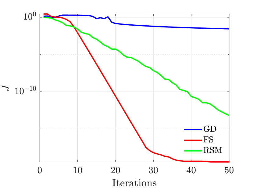
Figure 4: XOR approximation. Cost (12) computed with the neural network gains optimized by each training method.

$x$	$\hat{y}_{\rm GD}$	$\hat{y}_{\rm FS}$	$\hat{y}_{\rm RSM}$
$\begin{bmatrix}0&0\end{bmatrix}$	$9.7155{\rm e}-02$	$9.3003{\rm e}-11$	$1.3148{\rm e}-07$
$\begin{bmatrix}0&1\end{bmatrix}$	$9.1980{\rm e}-01$	$1.0000{\rm e}+00$	$1.0000{\rm e}+00$
$\begin{bmatrix}1&0\end{bmatrix}$	$9.2056{\rm e}-01$	$1.0000{\rm e}+00$	$1.0000{\rm e}+00$
$\begin{bmatrix}1&1\end{bmatrix}$	$7.7451{\rm e}-02$	$6.5421{\rm e}-11$	$1.5650{\rm e}-07$

TABLE II: XOR approximation. Neural network predictions at the 50th iteration.

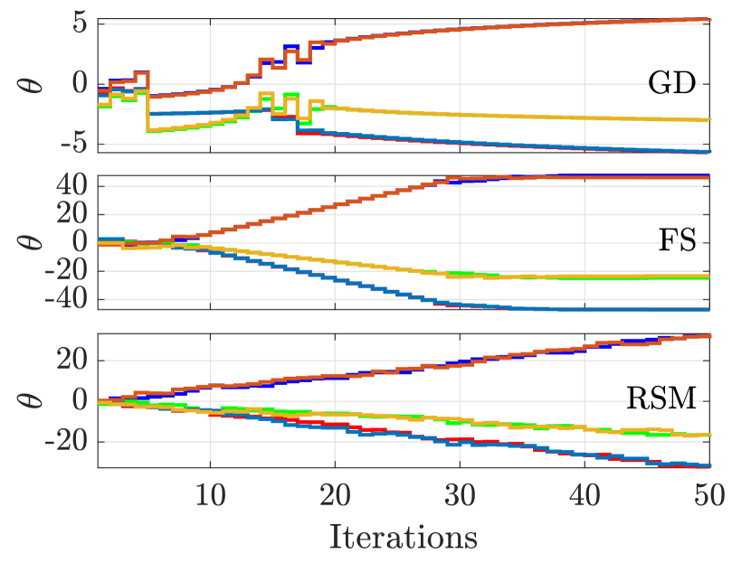
Figure 5: XOR approximation. Neural network gains optimized by each training method.

Example IV.2

[Trigonometric function approximation.] In this example, we train a neural network to approximate the sine function. Specifically, we consider a 2-layer neural network, with one neuron in each layer, that is,

$$x_{1} =x\in{\mathbb{R}},$$ (27)

$$x_{2} =N_{1}(x_{1},\Theta_{1})\in{\mathbb{R}},$$ (28)

$$y =N_{2}(x_{2},\Theta_{2})\in{\mathbb{R}}.$$ (29)

Note that $l_{x_{1}}=l_{x_{2}}=l_{y}=1$, and thus $l_{\theta_{1}}=2,$ $l_{\theta_{2}}=2,$ $\Theta_{1}\in{\mathbb{R}}^{2},$ and $\Theta_{2}\in{\mathbb{R}}^{2}.$

The training data is generated by selecting 100 linearly spaced values between $-\pi/2$ and $\pi/2.$ In gradient-descent method, we set learning rate $\alpha=0.01.$ In MATLAB’s fsolve routine, the function and step tolerance are set to $1{\rm e}-30.$ In the random search method, we generate a 500-member ensemble at each iteration and set the hypersphere radius $\alpha=1$. Figure 6 shows the cost (12) with the neural network gains optimized by each training method.

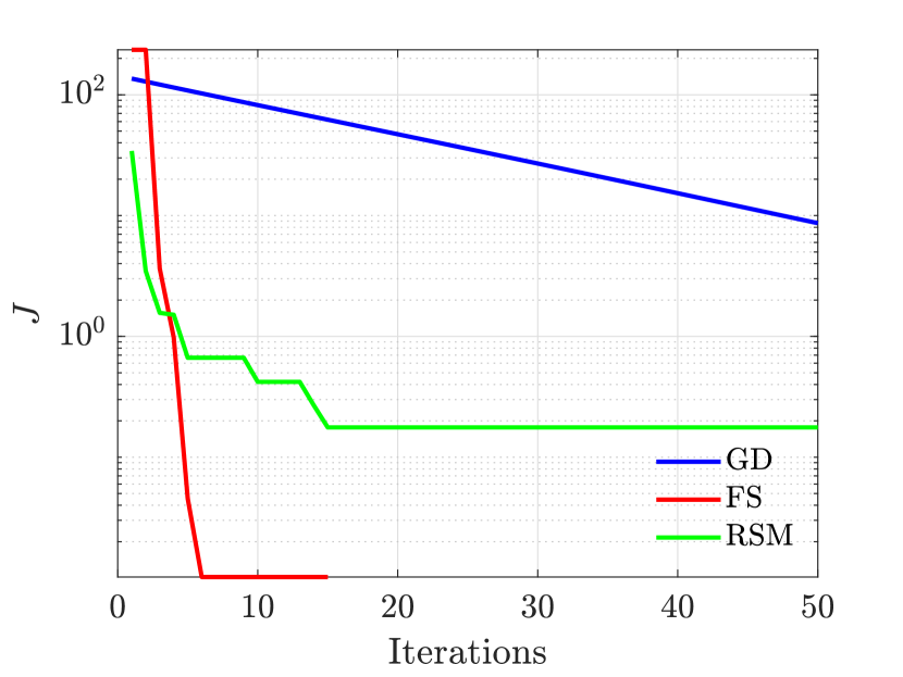
Figure 6: Sine approximation. Cost (12) computed with the neural network gains optimized by each training method.

To investigate the approximation accuracy of the three trained neural network, we compute the error $|y-\hat{y}|,$ where $y=\sin(x)$ and $\hat{y}=NN(x,(\Theta_{1},\Theta_{2})),$ at randomly generated values of $x$ between $-\pi/2$ and $\pi/2.$ Figure 7 shows the error with the neural network gains obtained at the 50th iteration. Figure 8 shows the neural network gains after each iteration of training with all three methods. Similar to the previous example, the fsolve routine, which solves the nonlinear system of equations (24), outperforms the other two training methods in terms of convergence rate and prediction accuracy. $\diamond$

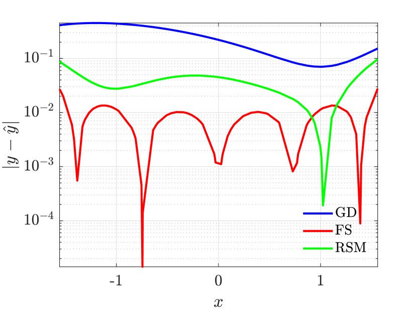
Figure 7: Sine approximation. Neural network prediction error at the 50th iteration.

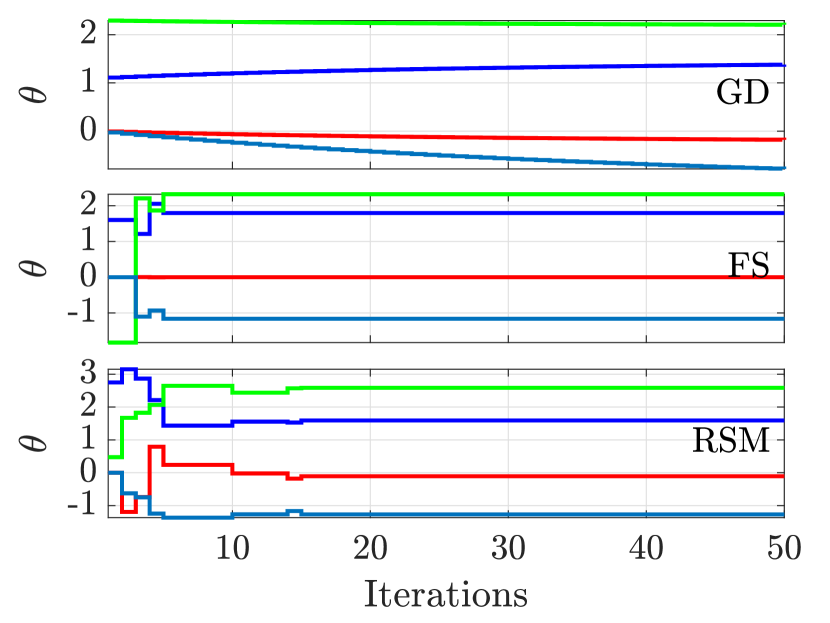
Figure 8: Sine approximation. Neural network gains optimized by each training method.

Example IV.3

[Handwritten digit identification.] In this example, we train a neural network to identify handwritten numbers. To keep computational requirements low, we consider the problem of identifying the integers $0,$ $1,$ and $2.$ We consider a 2-layer neural network with 30 neurons in the first layer and 3 neurons in the second layer. The activation functions are chosen to be ReLU in the first layer and sigmoid in the second layer. Therefore,

$$x_{1} =x\in{\mathbb{R}}^{784},$$ (30)

$$x_{2} =N_{1}(x_{1},\Theta_{1})\in{\mathbb{R}}^{30},$$ (31)

$$y =N_{2}(x_{2},\Theta_{2})\in{\mathbb{R}}^{3}.$$ (32)

Note that $l_{x_{1}}=784,$ $l_{x_{2}}=30,$ $l_{y}=3$, and thus $l_{\theta_{1}}=785,$ $l_{\theta_{2}}=31,$ $\Theta_{1}\in{\mathbb{R}}^{785\times 30},$ and $\Theta_{2}\in{\mathbb{R}}^{31\times 3}.$

The training data set consists of 30 labeled images corresponding to the digits $0,$ $1,$ and $2$ in the MNIST data set. We use the gradient-descent method implemented in TensorFlow with a learning rate of $\alpha=0.7$. In MATLAB’s fsolve, the default optimization options are used. In the random search method, we generate a 5000-member ensemble at each iteration and set the hypersphere radius $\alpha=1$. Figure 9 shows the cost (12) with the neural network gains optimized by each training method. Note that the cost $J$ drops to exactly $0$ at the 13th iteration in the random search method, which is rare in typical parameter fitting problems, but is plausible due to a small number of training samples and a large number of parameters being fitted.

To determine the accuracy of the trained neural network, we use the three trained neural networks to identify 100 samples of digits 0, 1, and 2. Note that we use the three trained neural networks to identify digits from a validation dataset that is different from the training dataset. Table III shows the neural network predictions of sample handwritten digits. Figure 10 shows the number of correct identifications for each of the digits predicted by the three networks. Note that, unlike the previous examples, the neural network trained by the random search method outperforms the other two networks. $\diamond$

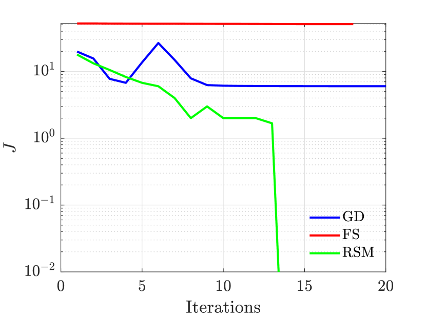
Figure 9: Digit identification. Cost (12) computed with the neural network gains optimized by each training method.

$x$	$y$	$\hat{y}_{\mathrm{GD}}$	$\hat{y}_{\mathrm{FS}}$	$\hat{y}_{\mathrm{RSM}}$
	$\begin{bmatrix}1\\ 0\\ 0\end{bmatrix}$	$\begin{bmatrix}0.152\\ 0.139\\ 0.149\end{bmatrix}$	$\begin{bmatrix}1.000\\ 0.000\\ 1\end{bmatrix}$	$\begin{bmatrix}1\\ 0.000\\ 0.000\\ \end{bmatrix}$
	$\begin{bmatrix}0\\ 1\\ 0\end{bmatrix}$	$\begin{bmatrix}1.000\\ 1.000\\ 1.000\\ \end{bmatrix}$	$\begin{bmatrix}1\\ 1.000\\ 0.986\end{bmatrix}$	$\begin{bmatrix}0\\ 1\\ 0.000\end{bmatrix}$
	$\begin{bmatrix}0\\ 0\\ 1\end{bmatrix}$	$\begin{bmatrix}1.000\\ 1.000\\ 1.000\end{bmatrix}$	$\begin{bmatrix}1\\ 0.015\\ 1.000\end{bmatrix}$	$\begin{bmatrix}0.000\\ 0.000\\ 1\end{bmatrix}$

TABLE III: Digit identification. Neural network predictions of sample handwritten digits. Note that the digits are sampled from a validation dataset that is different from the training dataset.

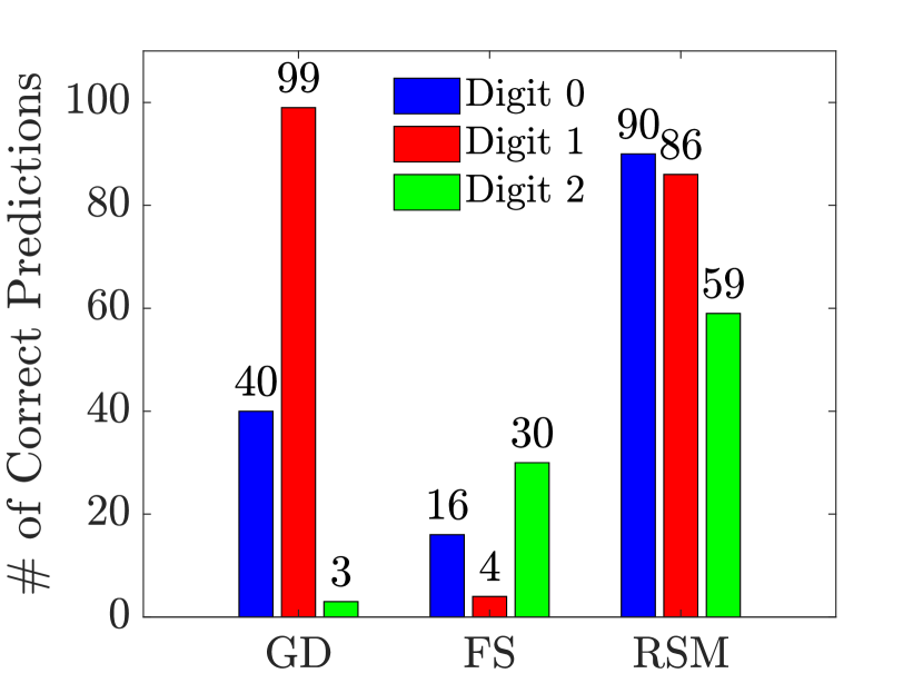
Figure 10: Digit identification. The number of correct predictions made by the three trained neural networks out of 100 validation samples of each digit.

V Conclusion

This paper presented a compact, matrix-based representation of neural networks in a self-contained tutorial fashion. The neural networks are represented as a composition of several nonlinear mathematical functions. Three numerical methods, one based on gradient-descent and two gradient-free, are reviewed for training a neural network. The reviewed training methods are applied to three typical machine learning problems. Surprisingly, the neural networks trained with the gradient-free methods outperformed the neural network trained with the widely used gradient-based optimizer.

Useful Facts

The following facts review the well-known results from multivariable calculus.

Fact V.1

Derivatives of scalar functions with respect to vectors. Let $a\in{\mathbb{R}}^{n},$ $A\in{\mathbb{R}}^{n\times n},$ and $f\colon{\mathbb{R}}^{n}\to{\mathbb{R}}.$ Let $x\in{\mathbb{R}}^{n}$. Then,

$$\dfrac{\partial x^{\rm T}a}{\partial x} =\dfrac{\partial a^{\rm T}x}{\partial x}=a^{\rm T}\in{\mathbb{R}}^{1\times n},$$ (33)

$$\dfrac{\partial x^{\rm T}Ax}{\partial x} =2x^{\rm T}A\in{\mathbb{R}}^{1\times n},$$ (34)

$$\dfrac{\partial f}{\partial x} =\begin{bmatrix}\dfrac{\partial f}{\partial x_{1}}&\cdots&\dfrac{\partial f}{\partial x_{n}}\end{bmatrix}\in{\mathbb{R}}^{1\times n}.$$ (35)

Fact V.2

Derivatives of vector functions with respect to vectors. Let $A\in{\mathbb{R}}^{m\times n}$ and $f\colon{\mathbb{R}}^{n}\to{\mathbb{R}}^{m}.$ Let $x\in{\mathbb{R}}^{n}$ Then,

$$\dfrac{\partial Ax}{\partial x} =A\in{\mathbb{R}}^{m\times n},$$ (36)

$$\dfrac{\partial f}{\partial x} =\begin{bmatrix}\dfrac{\partial f_{1}}{\partial x_{1}}&\cdots&\dfrac{\partial f_{1}}{\partial x_{n}}\\ \vdots&\ddots&\vdots\\ \dfrac{\partial f_{m}}{\partial x_{1}}&\cdots&\dfrac{\partial f_{m}}{\partial x_{n}}\end{bmatrix}\in{\mathbb{R}}^{m\times n}.$$ (37)

Fact V.3

Derivatives of scalar functions with respect to matrices. Let $a\in{\mathbb{R}}^{n},$ $b\in{\mathbb{R}}^{m},$ $A\in{\mathbb{R}}^{n\times n},$ and $f\colon{\mathbb{R}}^{n\times m}\to{\mathbb{R}}.$ Let $X\in{\mathbb{R}}^{n\times m}$. Then,

$$\dfrac{\partial a^{\rm T}Xb}{\partial X} =ba^{\rm T}\in{\mathbb{R}}^{m\times n},$$ (38)

$$\dfrac{\partial f}{\partial X} =\begin{bmatrix}\dfrac{\partial f}{\partial X_{11}}&\cdots&\dfrac{\partial f}{\partial X_{n1}}\\ \vdots&\ddots&\vdots\\ \dfrac{\partial f}{\partial X_{1m}}&\cdots&\dfrac{\partial f}{\partial X_{mn}}\end{bmatrix}\in{\mathbb{R}}^{m\times n}.$$ (39)

Fact V.4

The derivative of the sigmoid function $\sigma(z)=\dfrac{1}{1+e^{-z}}$ is given by

$$\sigma_{z}(z)\stackrel{{\scriptstyle\triangle}}{{=}}\dfrac{\partial\sigma}{\partial z}=\sigma(z)[1-\sigma(z)].$$ (40)

Fact V.5

Chain rule. Let $f\colon{\mathbb{R}}^{m}\to{\mathbb{R}}^{p}$ and Define $h\colon{\mathbb{R}}^{n}\to{\mathbb{R}}^{p}$ as the composition of $f$ and $g$ , that is, $f\circ g,$ or, $h(x)=f(g(x)),$ where $x\in{\mathbb{R}}^{n}.$ Then,

$$\dfrac{\partial h}{\partial x}=\dfrac{\partial h}{\partial y}\dfrac{\partial y}{\partial x},$$ (41)

where $y\stackrel{{\scriptstyle\triangle}}{{=}}g(x)\in{\mathbb{R}}^{m}.$ Note that $\dfrac{\partial y}{\partial x}\in{\mathbb{R}}^{m\times n}$ and $\dfrac{\partial h}{\partial y}\in{\mathbb{R}}^{p\times m}$, and thus $\dfrac{\partial h}{\partial x}\in{\mathbb{R}}^{p\times n}.$

The following results apply well-known multivariable calculus results to multivariable functions typically used in neural network training.

Fact V.6

Let $x\in{\mathbb{R}}^{l_{x}}$ and define $\chi\stackrel{{\scriptstyle\triangle}}{{=}}\begin{bmatrix}x^{\rm T}&1\end{bmatrix}^{\rm T}.$ Then,

$$\dfrac{\partial\chi}{\partial x}={\mathcal{J}}_{l_{x}},$$ (42)

where

$${\mathcal{J}}_{l_{x}}\stackrel{{\scriptstyle\triangle}}{{=}}\begin{bmatrix}I_{l_{x}}\\ 0_{1\times{l_{x}}}\end{bmatrix}\in{\mathbb{R}}^{l_{x}+1\times l_{x}}.$$ (43)

Fact V.7

Let $z\stackrel{{\scriptstyle\triangle}}{{=}}{\mathcal{L}}(x,\theta)=\chi^{\rm T}\theta,$ where $\theta\in{\mathbb{R}}^{l_{\theta}}.$ Note that $l_{\theta}=l_{x}+1.$ Let $\sigma\colon{\mathbb{R}}\to{\mathbb{R}}.$ Then,

$$\dfrac{\partial\sigma({\mathcal{L}}(x,\theta)}{\partial{\theta}} =\dfrac{\partial\sigma}{\partial{z}}\dfrac{\partial z}{\partial{\theta}}=\sigma_{z}(z)\chi^{\rm T}\in{\mathbb{R}}^{1\times l_{\theta}},$$ (44)

and

$$\dfrac{\partial\sigma({\mathcal{L}}(x,\theta)}{\partial{x}} =\dfrac{\partial\sigma}{\partial{z}}\dfrac{\partial z}{\partial\chi}\dfrac{\partial{\chi}}{\partial x}=\sigma_{z}(z)\theta^{\rm T}{\mathcal{J}}_{l_{x}}\in{\mathbb{R}}^{1\times l_{x}}.$$ (45)

Fact V.8

Let $z\stackrel{{\scriptstyle\triangle}}{{=}}{\mathcal{L}}(x,\Theta e)=\chi^{\rm T}\Theta e,$ where $\Theta\in{\mathbb{R}}^{l_{\theta}\times\ell}.$ Note that $e\in{\mathbb{R}}^{\ell}.$ Then,

$$\dfrac{\partial\sigma({\mathcal{L}}(x,\Theta e_{j})}{\partial{\Theta}} =\dfrac{\partial\sigma}{\partial{z}}\dfrac{\partial z}{\partial{\Theta}}=\sigma_{z}(z)e\chi^{\rm T}\in{\mathbb{R}}^{\ell\times l_{\theta}}.$$ (46)

Fact V.9

Let

$$N(x,\Theta)=\begin{bmatrix}\sigma({\mathcal{L}}(x,\Theta e_{1})\\ \vdots\\ \sigma({\mathcal{L}}(x,\Theta e_{\ell})\end{bmatrix}\in{\mathbb{R}}^{\ell},$$ (47)

where $\Theta=\begin{bmatrix}\theta_{1}&\cdots&\theta_{\ell}\end{bmatrix}\in{\mathbb{R}}^{l_{x}+1\times\ell}.$ Then, for $j=\{1,2,\ldots,\ell\},$

$$\dfrac{\partial N}{\partial\theta_{j}} =\begin{bmatrix}\vdots\\ \dfrac{\partial\sigma({\mathcal{L}}(x,\theta_{j})}{\partial{\theta_{j}}}\\ \vdots\\ \end{bmatrix}=\sigma_{z}(z_{j})e_{j}\chi^{\rm T}\in{\mathbb{R}}^{\ell\times l_{\theta}},$$ (48)

$$\dfrac{\partial N}{\partial x} =\begin{bmatrix}\vdots\\ \dfrac{\partial\sigma({\mathcal{L}}(x,\theta_{j})}{\partial{x}}\\ \vdots\end{bmatrix}=\begin{bmatrix}\vdots\\ \sigma_{z}(z_{j})\theta_{j}^{\rm T}{\mathcal{J}}_{l_{x}}\\ \vdots\end{bmatrix}$$

$$=\Lambda(x,\Theta)\Theta^{\rm T}{\mathcal{J}}_{l_{x}}\in{\mathbb{R}}^{\ell\times l_{x}},$$ (49)

where

$$\Lambda(x,\Theta)={\rm diag\ }(\sigma_{z}({\mathcal{L}}(x,\theta_{1})),\ldots,\sigma_{z}({\mathcal{L}}(x,\theta_{\ell})))\in{\mathbb{R}}^{\ell\times\ell}.$$ (50)

Fact V.10

Backpropagation. Let $z_{ij}={\mathcal{L}}(x_{i},\Theta_{i}e_{j}).$ Then, for $i<n+1,$

$$\dfrac{\partial y}{\partial\theta_{ij}} =\Theta_{n+1}^{\rm T}\prod_{q=n}^{i+1}\Lambda(x_{q},\Theta_{q})\Theta_{q}^{\rm T}{\mathcal{J}}_{l_{x_{q}}}\sigma_{z}(z_{ij})e_{j}x_{i}^{\rm T},$$ (51)

where $e_{j}$ is the $j$th column of the $\ell_{i}\times\ell_{i}$ identity matrix. Furthermore, for $i=n+1,$

$$\dfrac{\partial y}{\partial\theta_{n+1,j}} =\dfrac{\partial\Theta_{n+1}^{\rm T}x_{n+1}}{\partial\theta_{n+1,j}}=e_{j}x_{n+1}^{\rm T}.$$ (52)

Proof:

Note that, for $i<n+1,$

$$\dfrac{\partial y}{\partial\theta_{ij}} =\dfrac{\partial S(x_{n+1})}{\partial\theta_{ij}}$$

$$=\dfrac{\partial S(x_{n+1})}{\partial x_{n+1}}\dfrac{\partial x_{n+1}}{\partial\theta_{ij}}$$

$$=\Theta_{n+1}^{\rm T}\dfrac{\partial N_{n}(x_{n},\Theta_{n})}{\partial\theta_{ij}}$$

$$=\Theta_{n+1}^{\rm T}\dfrac{\partial N_{n}(x_{n},\Theta_{n})}{\partial x_{n}}\dfrac{\partial x_{n}}{\partial\theta_{ij}}$$

$$=\Theta_{n+1}^{\rm T}\Lambda(x_{n},\Theta_{n})\Theta_{n}^{\rm T}{\mathcal{J}}_{l_{x_{n}}}\dfrac{\partial N_{n-1}(x_{n-1},\Theta_{n-1})}{\partial\theta_{ij}}$$

$$=\Theta_{n+1}^{\rm T}\Lambda(x_{n},\Theta_{n})\Theta_{n}^{\rm T}{\mathcal{J}}_{l_{x_{n}}}\Lambda(x_{n-1},\Theta_{n-1})$$

$$\quad\cdot\Theta_{n-1}^{\rm T}{\mathcal{J}}_{l_{x_{n-1}}}\dfrac{\partial N_{n-2}(x_{n-2},\Theta_{n-2})}{\partial\theta_{ij}}$$

$$=\Theta_{n+1}^{\rm T}\prod_{q=n}^{i+1}\Lambda(x_{q},\Theta_{q})\Theta_{q}^{\rm T}{\mathcal{J}}_{l_{x_{q}}}\dfrac{\partial N_{i}(x_{i},\Theta_{i})}{\partial\theta_{ij}}$$

$$=\Theta_{n+1}^{\rm T}\prod_{q=n}^{i+1}\Lambda(x_{q},\Theta_{q})\Theta_{q}^{\rm T}{\mathcal{J}}_{l_{x_{q}}}\sigma_{z}(z_{ij})e_{j}x_{i}^{\rm T}.$$

∎

References

• [1] Pramila P Shinde and Seema Shah “A review of machine learning and deep learning applications” In 2018 Fourth international conference on computing communication control and automation (ICCUBEA), 2018, pp. 1–6 IEEE
• [2] James Andrew Bagnell, David Bradley, David Silver, Boris Sofman and Anthony Stentz “Learning for autonomous navigation” In IEEE Robotics & Automation Magazine 17.2 IEEE, 2010, pp. 74–84
• [3] Abera Tullu, Bedada Endale, Assefinew Wondosen and Ho-Yon Hwang “Machine learning approach to real-time 3D path planning for autonomous navigation of unmanned aerial vehicle” In Applied Sciences 11.10 MDPI, 2021, pp. 4706
• [4] Ian Goodfellow, Yoshua Bengio and Aaron Courville “Deep learning” MIT press, 2016
• [5] Dave Steinkraus, Ian Buck and PY Simard “Using GPUs for machine learning algorithms” In Eighth International Conference on Document Analysis and Recognition (ICDAR’05), 2005, pp. 1115–1120 IEEE
• [6] Sagar Sharma, Simone Sharma and Anidhya Athaiya “Activation functions in neural networks” In towards data science 6.12, 2017, pp. 310–316
• [7] Stephen Boyd, Stephen P Boyd and Lieven Vandenberghe “Convex optimization” Cambridge university press, 2004
• [8] Florian A Potra and Stephen J Wright “Interior-point methods” In Journal of computational and applied mathematics 124.1-2 Elsevier, 2000, pp. 281–302
• [9] William H Press, Saul A Teukolsky, William T Vetterling and Brian P Flannery “Numerical recipes 3rd edition: The art of scientific computing” Cambridge university press, 2007
• [10] Mikael Boden “A guide to recurrent neural networks and backpropagation” URL: https://wiki.eecs.yorku.ca/course_archive/2016-17/F/6327/_media/rn_dallas.pdf
• [11] MATLAB “fsolve: Solve system of nonlinear equations”, 2006 URL: https://www.mathworks.com/help/optim/ug/fsolve.html