Resource Sharing Through Multi-Round Matchings

Abstract

Applications such as employees sharing office spaces over a workweek can be modeled as problems where agents are matched to resources over multiple rounds. Agents’ requirements limit the set of compatible resources and the rounds in which they want to be matched. Viewing such an application as a multi-round matching problem on a bipartite compatibility graph between agents and resources, we show that a solution (i.e., a set of matchings, with one matching per round) can be found efficiently if one exists. To cope with situations where a solution does not exist, we consider two extensions. In the first extension, a benefit function is defined for each agent and the objective is to find a multi-round matching to maximize the total benefit. For a general class of benefit functions satisfying certain properties (including diminishing returns), we show that this multi-round matching problem is efficiently solvable. This class includes utilitarian and Rawlsian welfare functions. For another benefit function, we show that the maximization problem is NP-hard. In the second extension, the objective is to generate advice to each agent (i.e., a subset of requirements to be relaxed) subject to a budget constraint so that the agent can be matched. We show that this budget-constrained advice generation problem is NP-hard. For this problem, we develop an integer linear programming formulation as well as a heuristic based on local search. We experimentally evaluate our algorithms on synthetic networks and apply them to two real-world situations: shared office spaces and matching courses to classrooms.

1 Introduction

We consider resource allocation problems that arise in practical applications such as hot desking or shared work spaces (Varone and Beffa 2019; Cai and Khan 2010), classroom scheduling (Phillips et al. 2015), matching customers with taxicabs (Karamanis, Anastasiadis, and Angeloudis 2020; Kucharski and Cats 2020), and matching agricultural equipment with farms (Gilbert 2018; Rakhra and Singh 2020). In such scenarios, many agents (individuals, cohorts, farms, or in general, entities) are competing for a limited number of time-shared resources. In our formulation, an agent can be matched to at most one resource in any time slot, but might want to be matched in more than one time slot. Agents may have some restrictions that limit the set of resources to which they can be matched or possible time slots in which they can be matched. Any resource whose specifications do not meet an agent’s restrictions is incompatible with that agent.

In light of the COVID-19 pandemic, such resource allocation problems have become as important as ever. For example, social-distancing requirements (such as maintaining a six-foot separation between individuals) led to a dramatic decrease in the number of individuals who can occupy an enclosed space, whether it is a classroom (District Management Group 2020; Enriching Students 2020), workspace (Parker 2020) or visitation room (Wong 2021).

We model this resource allocation problem as a $k$-round matching problem on a bipartite graph, where the two node sets represent the agents and resources respectively. We assume that the rounds are numbered 1 through $k$, and each round matches a subset of agents with a subset of resources. Each agent specifies the set of permissible rounds in which it can participate and the desired number of rounds (or matchings) in which it needs to be assigned a resource. Consider for example a classroom scheduling for a workweek ($k=5$). Each lecturer who wants to schedule class sessions for her courses specifies the number of sessions she would like to schedule and the possible weekdays. There may also be additional requirements for classrooms (e.g., room size, location, computer lab). As a result, some agent-resource pairs become incompatible. The Principal’s objective is to find a set of at most $k$ matchings satisfying all the requirements, if one exists. In the classroom scheduling example, the existence of such a set means that there exists a solution where each lecturer receives the desired number of sessions on the desired days.

We refer to this as the multi-round matching problem (MRM). We consider two additional problem formulations to cope with the situation when a solution satisfying all the requirements does not exist.

In the first formulation, an agent receives a benefit (or reward) that depends on the number of rounds where it is matched, and the objective is to find a solution that maximizes the sum of the benefits over all agents. We refer to this as the multi-round matching for total benefit maximization problem (abbreviated as MaxTB-MRM). When applying this formulation to the classroom scheduling example, it is possible to find a solution in which the number of assigned sessions is maximized (by maximizing the corresponding utility function). Alternatively, we can also find a solution in which the minimal assignment ratio for a lecturer (i.e., the number of assigned sessions divided by the number requested) is maximized.

In the second formulation, the objective is to generate suitable advice to each agent to relax its resource requirements so that it becomes compatible with previously incompatible resources. However, the agent incurs a cost to relax its restrictions (e.g., social distancing requirements not met, increase in travel time). So, the suggested advice must satisfy the budget constraints that are chosen by the agents. In other words, the goal of this problem is to suggest relaxations to agents’ requirements, subject to budget constraints, so that in the new bipartite graph (obtained after relaxing the requirements), all the agents’ requirements are satisfied. In scheduling classrooms, for example, the Principal may require that some lecturers waive a subset of their restrictions (e.g., having a far-away room) so that they can get the number of sessions requested. We refer to this to as the advice generation for multi-round matching problem (abbreviated as AG-MRM).

Summary of contributions:

(a) An efficient algorithm for MaxTB-MRM. For a general class of benefit functions that satisfy certain properties including monotonicity (i.e., the function is non-decreasing with increase in the number of rounds) and diminishing returns (i.e., increase in the value of the function becomes smaller as the number of rounds is increased), we show that the MaxTB-MRM problem can be solved efficiently by a reduction to the maximum weighted matching problem. A simple example of such a function (where each agent receives a benefit of 1 for each round in which it is matched) represents a utilitarian social welfare function (Viner 1949). Our efficient algorithm for this problem yields as a corollary an efficient algorithm for the MRM problem mentioned above. Our algorithm can also be used for a more complex benefit function that models a Rawlsian social welfare function (Rawls 1999; Stark 2020), where the goal is to maximize the minimum satisfaction ratio (i.e., the ratio of the number of rounds assigned to an agent to the requested number of rounds) over all the agents.

(b) Maximizing the number of satisfied agents. Given a multi-round matching, we say that an agent is satisfied if the matching satisfies all the requirements of the agent. The objective of finding a multi-round matching that satisfies the largest number of agents can be modeled as the problem of maximizing the total benefit by specifying a simple benefit function for each agent. However, such a benefit function doesn’t have the diminishing returns property. We show that this optimization problem (denoted by MaxSA-MRM) is NP-hard, even when each agent needs to be matched in at most three rounds. This result points out the importance of the diminishing returns property in obtaining an efficient algorithm for maximizing the total benefit.

(c) Advice generation. We show that AG-MRM is NP-hard even when there is only one agent who needs to be matched in two or more rounds. Recall that the AG-MRM problem requires that each agent must be satisfied (i.e., assigned the desired number of rounds) in the new compatibility graph (obtained by relaxing the suggested restrictions). It is interesting to note that the hardness of AG-MRM is due to the advice generation part and not the computation of matching. (Without the advice generation part, the AG-MRM problem corresponds to MRM on a given compatibility graph, which is efficiently solvable as mentioned above.) The hardness of AG-MRM directly implies the hardness of the problem (denoted by AG-MaxSA-MRM) where the generated advice must lead to a matching that satisfies the maximum number of agents. We present two solution approaches for the AG-MaxSA-MRM problem: (i) an integer linear program (ILP-AG-MaxSA-MRM) to find an optimal solution and (ii) a pruned local search heuristic (PS-AG-MaxSA-MRM) that uses our algorithm for MRM to generate solutions of good quality.

(d) Experimental results. We present a back-to-the-lab desk-sharing study that has been conducted in the AI lab at a university to facilitate lab personnel intending to return to the work place during the COVID-19 epidemic. This study applies our algorithms to guide policies for returning to work. In addition, we present an experimental evaluation of our algorithms on several synthetic data sets as well as on a data set for matching courses to classrooms.

Table 1 shows the list of problems considered in our work and our main results.

Problem	Results
MaxTB-MRM	Efficient algorithm for a general class of benefit functions. An efficient algorithm for the MRM problem is a corollary.
MaxSA-MRM	NP-hard (reduction from Minimum Vertex Cover for cubic graphs)
AG-MRM	NP-hard (reduction from Minimum Set Cover)
AG-MaxSA-MRM	ILP and a local search heuristic for AG-MaxSA-MRM

Table 1: Overview of problems and main results

2 Related Work

Resource allocation in multi-agent systems is a well-studied area (e.g., (Chevaleyre et al. 2006; Gorodetski, Karsaev, and Konushy 2003; Dolgov and Durfee 2006)). The general focus of this work is on topics such as how agents express their requirements, algorithms for allocating resources and evaluating the quality of the resulting allocations. Some complexity and approximability issues in this context are discussed in Nguyen et al. (2013). Zahedi et al. (2020) study the allocation of tasks to agents so that the task allocator can answer queries on counterfactual allocations.

Babaei et al. (2015) presented a survey of approaches to solving timetabling problems that assign university courses to spaces and time slots, avoiding the violation of hard constraints and trying to satisfy soft constraints as much as possible. A few papers proposed approaches to exam timetabling (e.g., Leite et al. (2019), Elley (2006)). Other work addressed timetabling for high schools (e.g., Fonseca et al. (2016) and Tan et al. (2021)). However, the constraints allowed in the various timetabling problem variations are much more complex than in our setting.

Variants of multi-round matching have been considered in game theoretic settings. Anshelevich et al. (2013) consider an online matching algorithm where incoming agents are matched in batches. Liu (2020) considers matching a set of long-lived players (akin to resources in our setting) to short-lived players in time-slots. These two works focus on mechanism design to achieve stability and maximize social welfare. Gollapudi et al. (2020) and also Caragiannis and Narang (2022) consider repeated matching with the objective of achieving envy-freeness. However, the latter only considers the case of perfect matching, where agents are matched exactly once in each round. Sühr et al. (2019) considered optimizing fairness in repeated matchings motivated by applications to the ride-hailing problem.

Zanker et al. (2010) discuss the design and evaluation of recommendation systems that allow users to specify soft constraints regarding products of interest. A good discussion on the design of constraint-based recommendation systems appears in Felfernig et al. (2011).

Zhou and Han (2019) propose an approach for a graph-based recommendation system that forms groups of agents with similar preferences to allocate resources. Trabelsi et al. (2022a, 2022b) discussed the problem of advising an agent to modify its preferences so that it can be assigned a resource in a maximum matching. In this work, however, the advice is given to a single agent and only one matching is generated.

To our knowledge, the problems studied in our paper, namely finding multi-round matchings that optimize general benefit functions and advising agents to modify their preferences so that they can be assigned resources in such matchings, have not been addressed in the literature.

3 Definitions and Problem Formulation

3.1 Preliminaries

Agents, resources and matching rounds

Let $\mbox{$X$}{}=\{x_{1},x_{2},\ldots,x_{n}\}$ be a set of $n$ agents and $\mbox{$Y$}{}=\{y_{1},y_{2},\ldots,y_{m}\}$ a set of $m$ resources. The objective of the system or the Principal is to generate $k$ matchings $M_{1},\ldots,M_{k}$ of agents to resources, which we henceforth refer to as a $\mathbf{k}$-round matching. However, each agent has certain requirements that need to be satisfied. Firstly, each agent $x_{i}$ specifies a set $K_{i}\subseteq\{1,2,\ldots,k\}$ and wants to be matched in $\rho_{i}$ rounds from $K_{i}$.

Restrictions and Restrictions Graph

In addition to round preferences, agents may have restrictions due to which they cannot be matched to certain (or all) resources. We model this using an $XY$ bipartite graph with multiple labels on edges, with each label representing a restriction. We refer to this graph as the restrictions graph and denote it as $G_{R}(X,Y,E_{R})$, where $E_{R}$ is the edge set. Each edge $e\in E_{R}$ is associated with a set $\Gamma_{e}$ of agent-specific labels representing restrictions.

Compatibility Graph

Let $\mbox{$\mathcal{C}$}_{i}$ denote the set of edge labels or restrictions associated with agent $x_{i}$. Suppose a set $C\subseteq\mbox{$\mathcal{C}$}_{i}$ of restrictions makes resource $y_{j}$ incompatible with $x_{i}$, we draw a labeled edge $\{x_{i},y_{j}\}$ with labels in $C$. We say that $C$ is the restrictions set for the edge $\{x_{i},y_{j}\}$. To make $x_{i}$ compatible with $y_{j}$, all the restrictions in $C$ must be removed. There can be hard constraints due to which $y_{j}$ can never be compatible with $x_{i}$ even if all the restrictions are removed, in which case, $x_{i}$ and $y_{j}$ are not adjacent in $G_{R}$. Let $E\subseteq E_{R}$ be the set of all edges for which the restrictions set is empty. The corresponding subgraph $G(X,\,Y,\,E)$ is called the compatibility graph. An example showing a restrictions graph, a compatibility graph and multi-round matching appears as Figure 1. This example (Figure 1) is motivated by the Lab-Space application considered in this work. There are lab members (agents) who need to be assigned rooms (resources) – one person per room – on five days (i.e., $k=5$) with some preferences for space and days. Restrictions on each edge are induced by the mismatch between agent preferences and resource properties. For example, $x_{1}$ requires a big room, while $y_{2}$ is small. Therefore, we add a restriction (or label) $\mathtt{big}_{1}$ to the edge $\{x_{1},y_{2}\}$. The restrictions graph for this problem is shown followed by a multi-round matching solution.

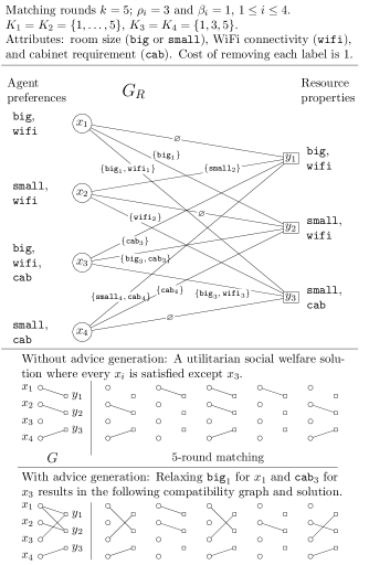
Figure 1: An example: A restrictions graph $G_{R}$ is induced by agent preferences and resource attributes. The first multi-round matching solution corresponds to the compatibility without the advice generation component. Not all agents are satisfied. The second solution satisfies all agents.

Costs for restrictions removal

For each restriction $c_{i}^{t}$, there is a positive cost $\psi_{i}^{t}$ associated with removing $c_{i}^{t}$. To remove any set of labels, we use an additive cost model, i.e., for any $C\subseteq\mbox{$\mathcal{C}$}_{i}$, the cost incurred by agent $x_{i}$ for removing all the restrictions in $C$ is $\sum_{c_{i}^{t}\in C}\psi_{i}^{t}$. An agent $x_{i}$ is satisfied if it is matched in $\rho_{i}$ rounds belonging to the set $K_{i}$. Now, we formally define the multi-round matching and advice generation problems.

3.2 Multi-round Matching

We begin with a definition of the basic multi-round matching problem (MRM) and discuss other versions.

Multi-Round Matching (MRM)

Instance: A compatibility graph $G(X,\,Y,\,E)$, number of rounds of matching $k$; for each agent $x_{i}$, the set of permissible rounds $K_{i}\subseteq\{1,\ldots,k\}$, the number of rounds $\rho_{i}\leq|K_{i}|$ in which $x_{i}$ wants to be matched.

Requirement: Find a $k$-round matching that satisfies all the agents (i.e., one that meets the requirements of all the agents), if one exists.

Since a solution may not exist for a given instance of the MRM problem, we consider an extension that uses a benefit (or utility) function for each agent. For each agent $x_{i}$, the benefit function $\mu_{i}:\{0,1,\ldots,\rho_{i}\}\rightarrow\mathbb{R}^{+}$, where $\mathbb{R}^{+}$ is the set of nonnegative real numbers, gives a benefit value $\mu_{i}(\ell)$ when the number of rounds assigned to $x_{i}$ is $\ell$, $0\leq\ell\leq\rho_{i}$. If a $k$-round matching assigns $\ell_{i}\leq\rho_{i}$ rounds to agent $x_{i}$, then the total benefit to all the agents is given by $\sum_{i=1}^{n}\mu_{i}(\ell_{i})$. We can now define a more general version of MRM.

Multi-Round Matching to Maximize Total Benefit (MaxTB-MRM)

Instance: A compatibility graph $G(X,\,Y,\,E)$, number of rounds of matching $k$; for each agent $x_{i}$, the set of permissible rounds $K_{i}\subseteq\{1,\ldots,k\}$, the number of rounds $\rho_{i}\leq|K_{i}|$ in which $x_{i}$ wants to be matched and the benefit function $\mu_{i}$.

Requirement: Find a $k$-round matching that maximizes the total benefit over all the agents.

As will be shown in Section 4, when the benefit functions satisfy some properties (including monotonicity and diminishing returns), the MaxTB-MRM problem can be solved efficiently. One such benefit function allows us to obtain an efficient algorithm for the MRM problem. Another benefit function allows us to define the problem of finding a $k$-round matching that maximizes the number of satisfied agents (abbreviated as MaxSA-MRM). However, this benefit function does not satisfy the diminishing returns property and so our efficient algorithm for MaxTB-MRM cannot be used for this problem. In fact, we show in Section 4 that the MaxSA-MRM problem is NP-hard.

3.3 Advice Generation

We define the multi-round matching advice generation problems, namely AG-MRM and AG-MaxSA-MRM.

Advice Generation for Multi-Round Matching
(AG-MRM)

Instance: A restrictions graph $G_{R}(X,Y,E_{R})$, number of rounds of matching $k$; for each agent $x_{i}$, the set of permissible rounds $K_{i}\subseteq\{1,\ldots,k\}$, the number of times $x_{i}$ wants to be matched $\rho_{i}\leq|K_{i}|$, and budget $\beta_{i}$; for each label $c_{i}^{t}\in\mbox{$\mathcal{C}$}_{i}$, a cost $\psi_{i}^{t}$ of removing that label. (Recall that $\mbox{$\mathcal{C}$}_{i}$ is the set of labels on the edges incident on agent $x_{i}$ in $G_{R}$.)

Requirement: For each agent $x_{i}$, is there a subset $\mbox{$\mathcal{C}$}^{\prime}_{i}\subseteq\mbox{$\mathcal{C}$}_{i}$ such that the following conditions hold? (i) The cost of removing all the labels in $\mbox{$\mathcal{C}$}^{\prime}_{i}$ for agent $x_{i}$ is at most $\beta_{i}$, and (ii) in the resulting compatibility graph, there exists a $k$-round matching such that all agents are satisfied. If so, find such a $k$-round matching.

In Figure 1, the advice generation component is illustrated in the bottom-most panel. In this case, we note that there is a solution to the AG-MRM problem.

In general, since a solution may not exist for a given AG-MRM instance, it is natural to consider the version where the goal is to maximize the number of satisfied agents. We denote this version by AG-MaxSA-MRM.

Note:

For convenience, we defined optimization versions of problems MaxSA-MRM, AG-MRM and AG-MaxSA-MRM above. In subsequent sections, we show that these problems are NP-hard. It can be seen that the decision versions of these three problems are in NP; hence, these versions are NP-complete.

4 Maximizing Total Benefit

4.1 An Efficient algorithm for MaxTB-MRM

In this section, we present our algorithm for the MaxTB-MRM problem that finds a $k$-round matching that maximizes the total benefit over all the agents. This algorithm requires the benefit function for each agent to satisfy some properties. We now specify these properties.

Valid benefit functions:  For each agent $x_{i}$, $1\leq i\leq n$, let $\mu_{i}(\ell)$ denote the non-negative benefit that the agent $x_{i}$ receives if matched in $\ell$ rounds, for $\ell=0,1,2,\ldots,\rho_{i}$. Let $\delta_{i}(\ell)=\mu_{i}(\ell)-\mu_{i}(\ell-1)$ for $\ell=1,2,\ldots,\rho_{i}$. We say that the benefit function $\mu_{i}$ is valid if satisfies all of the following four properties: (P1) $\mu_{i}(0)=0$; (P2) $\mu_{i}$ is monotone non-decreasing in $\ell$; (P3) $\mu_{i}$ has the diminishing returns property, that is, $\mu_{i}(\ell)-\mu_{i}(\ell-1)\leq\mu_{i}(\ell-1)-\mu_{i}(\ell-2)$ for $2\leq\ell\leq\rho_{i}$; and (P4) $\delta_{i}(\ell)\leq 1$, for $\ell=1,2,\ldots,\rho_{i}$. Note that $\mu_{i}(\cdot)$ satisfies property P3 iff $\delta_{i}(\cdot)$ is monotone non-increasing in $\ell$. Property P4 can be satisfied by normalizing the increments in the benefit values.

Algorithm for MaxTB-MRM:  Recall that the goal of this problem is to find a multi-round matching that maximizes the total benefit over all the agents. The basic idea behind our algorithm is to reduce the problem to the maximum weighted matching problem on a larger graph. The steps of this construction are shown in Figure 2. Given a multi-round solution $\mathcal{M}$ that assigns $\ell_{i}$ rounds to agent $x_{i}$, $1\leq i\leq n$, let $\mathbb{B}(\mathcal{M})=\sum_{i=1}^{n}\mu_{i}(\ell_{i})$ denote the total benefit due to $\mathcal{M}$.

 

1. Given compatibility graph $G(X,Y,E)$, and for each agent $x_{i}$, permissible rounds $K_{i}$, the maximum number of rounds $\rho_{i}$, and benefit function $\mu_{i}(\cdot)$, create a new edge-weighted bipartite graph $G^{\prime}(X^{\prime},Y^{\prime},E^{\prime},w(\cdot))$ as follows. (The sets $X^{\prime}$, $Y^{\prime}$, and $E^{\prime}$ are all initially empty.)

   Node set $X^{\prime}$.

   For each agent $x_{i}\in X$ and each $h\in K_{i}$, add a node denoted by $x_{i}^{h}$ to $X^{\prime}$.

   Node set $Y^{\prime}$.

   For each resource $y_{j}\in Y$, add $k$ nodes denoted by $y_{j}^{h}$, where $h=1,2,\ldots,k$, to $Y^{\prime}$. These are called type-1 resource nodes. For every agent $x_{i}$, add $\rho_{i}$ nodes, denoted by $y^{2}_{i,p}$, where $p=1,2,\ldots,\rho_{i}$; these are called type-2 resource nodes. For every agent $x_{i}$, add $|K_{i}|-\rho_{i}$ nodes, denoted by let $y^{3}_{i,p}$, where $p=1,2,\ldots,|K_{i}|-\rho_{i}$; these are called type-3 resource nodes.

   Edge set $E^{\prime}$ and weight $w$.

   For every edge $\{x_{i},y_{j}\}\in E$ and each $h\in K_{i}$, add edge $\{x_{i}^{h},y_{j}^{h}\}$ to $E^{\prime}$ with weight $w(x_{i}^{h},y_{j}^{h})=1$. For each $h\in K_{i}$ and $p=1,\ldots,\rho_{i}$, add edge $\{x_{i}^{h},y^{2}_{i,p}\}$ with weight $w(x_{i}^{h},y^{2}_{i,p})=1-\delta_{i}(p)$. For each $h\in K_{i}$ and $p=1,\ldots,|K_{i}|-\rho_{i}$, add edge $\{x_{i}^{h},y^{3}_{i,p}\}$ with weight $w(x_{i}^{h},y^{3}_{i,p})=k+1$.

2. Find a maximum weighted matching $M^{*}$ in $G^{\prime}$.

3. Compute a collection of matchings $\mathcal{M}^{*}=\{M_{1},M_{2},\ldots,M_{k}\}$ for $G$ as follows. The sets $M_{1}$, $M_{2}$, $\ldots$, $M_{k}$ are initially empty. For each edge $e=\{x_{i}^{h},y_{j}^{h}\}\in M^{*}$ where $y_{j}^{h}$ is a type-1 resource, add the edge $\{x_{i},y_{j}\}$ to $M_{h}$.

Figure 2: Steps of Alg-MaxTB-MRM.

 

Now, we establish the following result.

Theorem 4.1.

Algorithm Alg-MaxTB-MRM (Figure 2) produces an optimal solution if every benefit function $\mu_{i}(\cdot)$ is valid.

We prove the above theorem through a sequence of definitions and lemmas.

Definition 4.2.

A matching $M$ of $G^{\prime}$ is saturated if $M$ includes (i) every node of $X^{\prime}$ and (ii) every node of $Y^{\prime}$ that represents a type-3 resource.

Lemma 4.3.

Given any maximum weight matching $M$ for $G^{\prime}$, a saturated maximum weight matching $M^{\prime}$ for $G^{\prime}$ with the same weight as $M$ can be constructed.

Proof sketch:  We first argue that every maximum weight matching of $G^{\prime}$ includes all type-3 resource nodes (since each edge incident on those nodes has a large weight). We then argue that other unmatched nodes of $X^{\prime}$ can be added suitably. For details, see Section A of the supplement.

Let the quantity $\lambda$ be defined by

$\lambda~{}=~{}\sum_{i=1}^{n}k(|K_{i}|-\rho_{i})+\sum_{i=1}^{n}\sum_{\ell=1}^{\rho_{i}}(1-\delta_{i}(\ell))$.

We use $\lambda$ throughout the remainder of this section. Note that $\lambda$ depends only on the parameters of the problem; it does not depend on the algorithm.

Lemma 4.4.

Suppose there is a saturated maximum weight matching $M$ for $G^{\prime}$ with weight $W$. Then, a solution to the MaxTB-MRM problem instance with benefit $W-\lambda$ can be constructed if every benefit function $\mu_{i}(\cdot)$ is valid.

Proof.

Given $M$, we compute a collection of matchings $\mathcal{M}=\{M_{1},M_{2},\ldots,M_{k}\}$ for $G$ as follows. For each edge $e=\{x_{i}^{h},y_{j}^{h}\}\in M$ where $y_{j}^{h}$ is a type-1 resource, add the edge $\{x_{i},y_{j}\}$ to $M_{h}$. First, we will show that each $M_{h}\in\mathcal{M}$ is a matching in $G$. Suppose $M_{h}$ is not a matching, then, there exists some $x_{i}$ or $y_{j}$ with a degree of at least two in $M_{h}$. We will prove it for the first case. The second case is similar. Suppose agent $x_{i}$ is adjacent to two resources $y_{j^{\prime}}$ and $y_{j^{\prime\prime}}$. This implies that in $M$, $x_{i}^{h}$ is adjacent to both $y_{j^{\prime}}^{h}$ and $y_{j^{\prime\prime}}^{h}$, contradicting the fact that $M$ is a matching in $G^{\prime}$. Hence, $\mathcal{M}$ is a valid solution to the MaxTB-MRM problem.

We now derive an expression for the weight $W$ of $M$. Since every type-3 resource is matched in $M$, the corresponding edges contribute $\sum_{i=1}^{n}k(|K_{i}|-\rho_{i})$ to $W$. For an agent $x_{i}$, let the number of edges to type-1 resources be $\gamma_{i}\leq\rho_{i}$. Each such edge is of weight $1$. The remaining $\rho_{i}-\gamma_{i}$ edges correspond to type-2 resources. Since each benefit function, $\mu_{i}$ satisfies the diminishing returns property, the incremental benefits $\delta_{i}(\cdot)$ are monotone non-increasing in the number of matchings. Thus, we may assume without loss of generality that the top $\rho_{i}-\gamma_{i}$ edges in terms of weight are in the maximum weighted matching $M$. This contributes $\sum_{\ell=1}^{\rho_{i}-\gamma_{i}}\big{(}1-\delta_{i}(\rho_{i}-\ell+1)\big{)}$ to $W$. Combining the terms corresponding to type-1 and type-2 resources, the contribution of agent $x_{i}$ to $W$ is $\gamma_{i}+\sum_{\ell=1}^{\rho_{i}-\gamma_{i}}\big{(}1-\delta_{i}(\rho_{i}-\ell+1)\big{)}=\sum_{\ell=1}^{\gamma_{i}}1+\sum_{\ell=\gamma_{i}}^{\rho_{i}}\big{(}1-\delta_{i}(\ell)\big{)}=\sum_{\ell=1}^{\rho_{i}}\big{(}1-\delta_{i}(\ell)\big{)}+\sum_{\ell=1}^{\gamma_{i}}\delta_{i}(\ell)$ . Summing this over all the agents, we get $W$ = $\sum_{i=1}^{n}k(|K_{i}|-\rho_{i})+\sum_{i=1}^{n}\sum_{\ell=1}^{\rho_{i}}\big{(}1-\delta_{i}(\ell)\big{)}+\sum_{i=1}^{n}\sum_{\ell=1}^{\gamma_{i}}\delta_{i}(\ell)=\lambda+\sum_{i=1}^{n}\mu_{i}(\gamma_{i})$. Since $\sum_{i=1}^{n}\mu_{i}(\gamma_{i})$ =  $\mathbb{B}(\mathcal{M})$, the lemma follows. ∎

Lemma 4.5.

Suppose there is a solution to the MaxTB-MRM problem instance with benefit $Q$. Then, there a saturated matching $M$ for $G^{\prime}$ with weight $Q+\lambda$ can be constructed.

Proof idea:  This proof uses an analysis similar to the one used in the proof of Lemma 4.4. For details, see Section A of the supplement.

Lemma 4.6.

There is an optimal solution to the MaxTB-MRM problem instance with benefit $Q^{*}$ if and only if there is a maximum weight saturated matching $M^{*}$ for $G^{\prime}$ with weight $Q^{*}+\lambda$.

Proof idea:  This is a consequence of Lemmas 4.4 and 4.5. For details see Section A of the supplement.

Theorem 4.1 is a direct consequence of Lemma 4.6.

We now estimate the running time of Alg-MaxTB-MRM.

Proposition 4.7.

Algorithm Alg-MaxTB-MRM runs in time $O(k^{3/2}(n+|E|)\sqrt{n+m}))$, where $n$ is the number of agents, $m$ is the number of resources, $k$ is the number of rounds and $E$ is the number of edges in the compatibility graph $G(X,Y,E)$.

Proof: See Section A of the supplement.

4.2 Maximizing Utilitarian Social Welfare

Here, we present a valid benefit function that models utilitarian social welfare. For each agent $x_{i}$, let $\mu_{i}(\ell)=\ell$, for $\ell{}=0,1,\ldots\rho_{i}$. It is easy to verify that this is a valid benefit function. Hence, the algorithm in Figure 2 can be used to solve the MaxTB-MRM problem with these benefit functions. An optimal solution in this case maximizes the total number of rounds assigned to all the agents, with agent $x_{i}$ assigned at most $\rho_{i}$ rounds, $1\leq i\leq n$.

This benefit function can also be used to show that the MRM problem (where the goal is to check whether there is a solution that satisfies all the agents) can be solved efficiently.

Proposition 4.8.

MRM problem can be solved in polynomial time.

Proof.

For each agent $x_{i}$, let the benefit function $\mu_{i}$ be defined by $\mu_{i}(\ell)=\ell$, for $0\leq\ell{}\leq\rho_{i}$. We will show that for this benefit function, the algorithm in Figure 2 produces a solution with total benefit $\sum_{i=1}^{n}\rho_{i}$ iff there is a solution to the MRM instance.

Suppose there is a solution to the MRM instance. We can assume (by deleting, if necessary, some rounds in which agents are matched) that each agent $x_{i}$ is assigned exactly $\rho_{i}$ rounds. Therefore, the total benefit over all the agents is $\sum_{i=1}^{n}\rho_{i}$. Since the maximum benefit that agent $x_{i}$ can get is $\rho_{i}$, this sum also represents the maximum possible total benefit. So, the total benefit of the solution produced by the algorithm in Figure 2 is $\sum_{i=1}^{n}\rho_{i}$.

For the converse, suppose the maximum benefit produced by the algorithm is equal to $\sum_{i=1}^{n}\rho_{i}$. It can be seen from Figure 2 that for any agent $x_{i}$, the algorithm assigns at most $\rho_{i}$ rounds. (This is due to the type-3 resource nodes for which all the incident edges have large weights.) Since the total benefit is $\sum_{i=1}^{n}\rho_{i}$, each agent $x_{i}$ must be assigned exactly $\rho_{i}$ rounds. Thus, the MRM instance has a solution. ∎

In subsequent sections, we will refer to the algorithm for MRM mentioned in the above proof as Alg-MRM.

4.3 Maximizing Rawlsian Social Welfare

Let $\gamma_{i}(\mathcal{M})$ denote the number of rounds assigned to agent $x_{i}$ in a multi-round solution $\mathcal{M}$. The minimum satisfaction ratio for $\mathcal{M}$ is defined as $\min_{i}\{\gamma_{i}(\mathcal{M})/\rho_{i}\}$. Consider the problem of finding a multi-round matching that maximizes the minimum satisfaction ratio. While the maximization objective of this problem seems different from the utilitarian welfare function, we have the following result.

Theorem 4.9.

There exists a reward function $\mu_{i}$ for each agent $x_{i}$ such that maximizing the total benefit under this function maximizes the Rawlsian social welfare function, i.e., it maximizes the minimum satisfaction ratio over all agents. Further, this reward function is valid and therefore, an optimal solution to the MaxTB-MRM problem under this benefit function can be computed in polynomial time.

To prove the theorem, we first show how the benefit function is constructed.

1. Let $F=\big{\{}k_{1}/k_{2}\mid k_{1},k_{2}\in\{1,\ldots,k\}~{}\mathrm{and}~{}k_{1}\leq k_{2}\big{\}}\cup\{0\}$.

2. Let $\pi:F\rightarrow\{1,\ldots,|F|\}$ give the index of each element in $F$ when sorted in descending order.

3. For each $q\in F$, let $\xi(q)=(nk)^{\pi(q)}/(nk)^{|F|}$, where $n$ is the number of agents and $k$ is the number of rounds. Note that each $\xi(q)\in(0,1]$.

4. The incremental benefit $\delta_{i}(\ell)$ for an agent $x_{i}$ for the $\ell$th matching is defined as $\delta_{i}(\ell)=\xi\big{(}(\ell-1)/\rho_{i}\big{)}$. Thus, the benefit function $\mu_{i}$ for agent $x_{i}$ is given by $\mu_{i}(0)=0$ and $\mu_{i}(\ell)=\mu_{i}(\ell-1)+\delta_{i}(\ell)$ for $1\leq\ell\leq\rho_{i}$.

It can be seen that $\mu_{i}$ satisfies properties P1, P2, and P4 of a valid benefit function. We now show that it also satisfies P3, the diminishing returns property.

Lemma 4.10.

For each agent $x_{i}$, the incremental benefit $\delta_{i}(\ell)$ is monotone non-increasing in $\ell$. Therefore, $\mu_{i}(\cdot)$ satisfies the diminishing returns property.

Proof.

By definition, for $\ell=1,\ldots,\rho_{i}-1$, $\delta_{i}(\ell)/\delta_{i}(\ell+1)=\xi\big{(}(\ell-1)/\rho_{i}\big{)}/\xi\big{(}\ell/\rho_{i}\big{)}\geq nk>1$, by noting that $\pi(\ell/\rho_{i})-\pi((\ell+1)/\rho_{i})\geq 1$. Hence, the lemma holds. ∎

To complete the proof of Theorem 4.9, we must show that any solution that maximizes the total benefit for the above benefit function also maximizes the minimum satisfaction ratio. This proof appears in Section A of the supplement.

4.4 Hardness of MaxSA-MRM

Here we consider the MaxSA-MRM problem, where the goal is to find a $k$-round matching to maximize the number of satisfied agents. A benefit function that models this problem is as follows. For each agent $x_{i}$, let $\mu_{i}(\ell)=0$ for $0\leq\ell{}\leq\rho_{i}-1$ and $\mu_{i}(\rho_{i})=1$. This function can be seen to satisfy properties P1, P2, and P4 of a valid benefit function. However, it does not satisfy P3, the diminishing returns property, since $\delta(\rho_{i}-1)=0$ while $\delta(\rho_{i})=1$. Thus, this is not a valid benefit function. This difference is enough to change the complexity of the problem.

Theorem 4.11.

MaxSA-MRM is NP-hard even when the number of rounds ($k$) is 3.

Proof idea:  We use a reduction from the Minimum Vertex Cover Problem for Cubic graphs which is known to be NP-complete (Garey and Johnson 1979). For details, see Section A of the supplement.

5 Advice Generation Problems

Here, we first point out that the AG-MRM and AG-MaxSA-MRM problems are NP-hard. We present two solution approaches for the AG-MaxSA-MRM problem, namely an integer linear program (ILP) formulation and a pruned-search-based optimization using Alg-MRM.

5.1 Complexity Results

Theorem 5.1.

The AG-MRM problem is NP-hard when there is just one agent $x_{i}$ for which $\rho_{i}>1$.

Proof idea. We use a reduction from the Minimum Set Cover (MSC) problem which is known to be NP-complete (Garey and Johnson 1979). For details, see Section B of the supplement.

Any solution to the AG-MRM problem must satisfy all the agents. Thus, the hardness of AG-MRM also yields the following:

Corollary 5.2.

AG-MaxSA-MRM is NP-hard.

5.2 Solution Approaches for AG-MaxSA-MRM

(a) ILP Formulation for AG-MaxSA-MRM:  This ILP formulation is presented in section B of the supplement.

(b) Alg-MRM guided optimization:  We describe a local search heuristic PS-AG-MaxSA-MRM for the MS-AG-MRM problem. It consists of three parts: (1) identification of relevant candidate sets of relaxations for each agent and edges in the restrictions graph (and hence the name pruned-search), (2) the valuation of an identified set of relaxations for all agents and (3) a local search algorithm.

In part (1), for each agent $x_{i}$, we first identify the sets of restrictions $\Gamma_{i}=\{\mbox{$\mathcal{C}$}^{\prime}_{i}\subseteq\mbox{$\mathcal{C}$}_{i}~{}|~{}$ Cost of removing all the labels in $\mbox{$\mathcal{C}$}^{\prime}_{i}$ for agent $x_{i}$ is $\leq$ $\beta_{i}\}$ to be considered for removal during the search. We choose a subcollection $\Gamma_{i}^{s}\subseteq\Gamma_{i}$ of sets based on the following criteria: (a) only Pareto optimal sets of constraints with respect to the budget are considered, i.e., if $\mbox{$\mathcal{C}$}^{\prime}_{i}\in\Gamma_{i}^{s}$, then there is no $c_{i}^{t}\in\mbox{$\mathcal{C}$}_{i}$ such that the cost of relaxation of $\mbox{$\mathcal{C}$}^{\prime}_{i}\cup\{c_{i}^{t}\}$ is less than or equal to $\beta_{i}$; (b) each $\mbox{$\mathcal{C}$}^{\prime}_{i}\in\Gamma_{i}^{s}$ is associated with a set of edges $E_{i}^{\prime}$ that will be added to the compatibility graph if $\mbox{$\mathcal{C}$}^{\prime}_{i}$ is relaxed; if $\mbox{$\mathcal{C}$}^{\prime}_{i}$ and $\mbox{$\mathcal{C}$}^{\prime\prime}_{i}$ are such that $E_{i}^{\prime\prime}\subseteq E_{i}^{\prime}$, then, we retain only $\mbox{$\mathcal{C}$}^{\prime}_{i}$; (c) if two sets of constraints cause the addition of the same set of edges to the compatibility graph, only one of them is considered.

In part (2), given a collection of relaxation sets, one for each unsatisfied agent, we apply Alg-MRM from Section 4 on the induced compatibility graph. The number of agents that are satisfied in the $k$-round solution obtained serves as the valuation for the collection of relaxation sets. In part (3), we use simulated annealing local search algorithm (Aarts and Korst 1989) for the actual search. The details of this implementation are in Section C of the supplement.

6 Experimental Results

We applied the algorithms developed in this work to several datasets. Evaluations were based on relevant benefit functions and computing time. We used at least 10 replicates for each experiment when needed (e.g., random assignment of attributes and while using PS-AG-MaxSA-MRM, which is a stochastic optimization algorithm). Error bars are provided in such instances. Implementation details are in Section C of the supplement. We considered two novel real-world applications (discussed below). Here, we describe the attributes of the datasets; the data itself and the code for running the experiments are available at https://github.com/yohayt/Resource-Sharing-Through-Multi-Round-Matchings.

Lab-Space application.

We conducted a back-to-the-lab desk sharing study in the AI lab at a university to facilitate lab personnel intending to return to in-person work during the COVID-19 epidemic. A survey was used to collect the preferences of lab members. The lab has 14 offices and 31 members. Six of the offices can accommodate two students each and the remaining eight can accommodate one student each. The agent restrictions are as follows: vicinity to the advisor’s room, presence of cabinet, WiFi connectivity, ambient noise, vicinity to the kitchen, room size, and vicinity to the bathroom. All agent preferences are generated from the survey as a function of the affinity (from 1 (low) to 5 (high)) they provide for each attribute. These affinities are also used as costs for attribute removal.

Course-Classroom dataset.

This dataset comes from a university¹ for the year 2018–2019. There are $144$ classrooms and $153$ courses. In the experiments, we focused on two hours on Tuesday and used all the courses that are scheduled in this time slot and all available classes. There were 142 courses and all the 144 classrooms were available for them. Each classroom has two attributes: its capacity and the region to which it belongs. Although the problem of assigning classrooms to courses is quite common (Phillips et al. 2015), we did not find any publicly available dataset that could be used here. The number of rounds of participation is chosen randomly between $1$ and $3$ as this data was not available. Also, to generate $K_{i}$, $\rho_{i}$ rounds are sampled uniformly followed by choosing the remaining days with probability $0.5$. We used 10 replicates for each experiment.

The generation of the restrictions and compatibility graphs from the agent preferences and resource attributes is described in detail in Section 6 of the supplement.

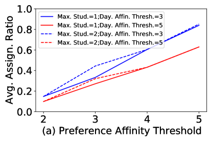
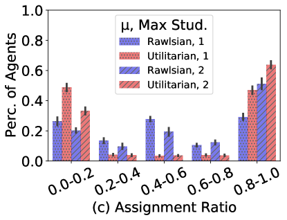
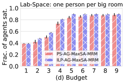
Figure 3: Lab-Space experiment results: (a) Average assignment ratio for different preference affinity thresholds; (b) Average assignment ratio when the number of resources is restricted; (c) Comparison of different welfare functions for resource probability $0.5$, and preference affinity and day affinity thresholds of $5$ and $2$ respectively; and (d) Evaluation of the advice generation algorithm for increasing budget. (See figure 6 for the case with two people per big room.)

Lab-Space multi-round matching.

Through this study, the head of the lab (Principal) wanted answers to the following questions: Is it possible to accommodate only one person per office? Is it possible to maximize the number of relevant assignments? Is it possible to achieve all this by satisfying as many preferences of lab members as possible? The number of rounds is $5$ (one for each weekday). We defined a preference affinity threshold. If the agent’s survey score for affinity (1-5) is at least as much as the threshold, then we add this preference as a constraint. Note that the compatibility graph generated for threshold $\tau$ is a subgraph of the one generated for $\tau+1$. The permissible sets of rounds $K_{i}$ are generated the same way. A day affinity threshold is set. If the agent’s preference for a weekday is lower than this threshold, then we do not add it to $K_{i}$. In Figure 3(a), we have results for maximizing the utilitarian social welfare for various compatibility graphs generated by adding constraints based on the agent’s affinity to each preference. We see that adhering strictly to the preferences of agents gives a very low average assignment ratio $\gamma_{i}/\rho_{i}$, where $\gamma_{i}$ is the number of rounds assigned to agent $x_{i}$ (who requested $\rho_{i}$ rounds). We considered two scenarios for large rooms: one or two students. We note that accommodating two students significantly improves the average assignment ratio. Adhering to the preferred days of students does not seem to have many costs, particularly when the preference affinity threshold is high. In Figure 3(b), we demonstrate how critical the current set of resources is for the functioning of the lab. We withheld only a portion of the resources (by sampling) to satisfy agent preferences. However, with just 60% of the resources, it is possible to get an average assignment ratio of $0.6$, albeit by ignoring most of the agent preferences. In Figure 3(c), we compare utilitarian social welfare with Rawlsian social welfare. We note that in the utilitarian welfare, many agents end up with a lower assignment ratio compared to Rawlsian, while the total number of matchings across rounds is the same. (A theorem in this regard is presented in Section D of the supplement; it states that for valid and monotone strictly increasing benefit functions, an optimal solution for total benefit also optimizes the total number of rounds assigned to agents.) Hence, from the perspective of fairness in agent satisfaction, the Rawlsian reward function performs better.

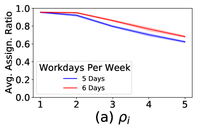
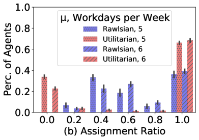
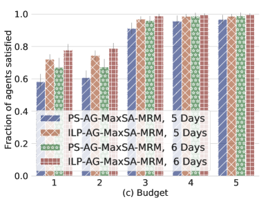
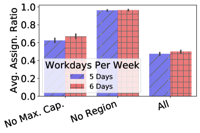
Figure 4: Course-Classroom experimental results: (a) Average assignment ratio vs. number of rounds required per agent; (b) Comparison of different welfare functions. (c) Evaluation of advice generation algorithm for increasing budget. (d) Importance of attributes.

Lab-Space advice generation.

From the results in Figure 3(d), we observe that there is a sharp increase in the number of agents satisfied for a budget of 4. In the data, there is a strong preference for WiFi (an average score of 4.3 out of 5), while more than 40% of the rooms have poor connectivity. When most of the agents relax this preference, they have access to many rooms. This partially explains the sharp increase in the number of matchings. We also observe that the performance of PS-AG-MaxSA-MRM is close to that of optimum (given by ILP-Max-AG-MRM).

Course-Classroom multi-round matching.

Here, we considered two scenarios: having classes (i) five days a week and (ii) six days a week. A six-day week can accommodate more courses while on the other hand, facilities have to be kept open for an additional day. The results of maximizing the utilitarian multi-round matching are in Figure 4(a). We observe that as $\rho_{i}$ is increased, the average assignment ratio decreases slowly. The difference between five and six days a week is not significant. Figure 4(b) compares utilitarian and Rawlsian reward functions. Unlike the Lab-Space results, here we clearly see that the minimum assignment ratio is higher in the former case.

Course-Classroom advice generation

In Figure 4(c) we observe that only for low budgets, the difference between five-day week and six-day week solutions is significant. In the same regime, we see a significant difference between PS-AG-MaxSA-MRM and ILP-Max-AG-MRM. By inspecting the solution sets, we observed that relaxing the region attribute is most effective in increasing the number of satisfied agents, while minimum capacity is least effective. To study the importance of different attributes, we conducted experiments where a single chosen attribute was omitted from the restrictions list. Figure 4(d) indicates that the region attribute has the most impact on the assignments ratio.

Scaling to larger networks.

To analyze the performance of the of the advice generation algorithms with respect to the size of the network, we experimented with complete bipartite graphs of various sizes. The results are in Section C of the supplement. In these experiments, we note that not only is the solution obtained using the PS-AG-MaxSA-MRM close to ILP-Max-AG-MRM, it is orders of magnitude faster.

7 Directions for Future Work

We conclude by mentioning a few directions for future work. One direction is to consider other models for producing compatibility graphs from restrictions graphs. (For example, an edge may be added to the compatibility graph if at least one label on that edge is removed.) It will also be interesting to consider the multi-round matching problems in an online setting, where the set of agents varies over time and compatibility is round-dependent. Finally, it is of interest to investigate approximation algorithms with provable performance guarantees for MaxSA-MRM and AG-MaxSA-MRM.

8 Acknowledgments

We thank the AAAI 2023 reviewers for their feedback. This research has been partially supported by the Israel Science Foundation under grant 1958/20, the EU Project TAILOR under grant952215, University of Virginia Strategic Investment Fund award number SIF160, and the US National Science Foundation grant OAC-1916805 (CINES).

Technical Supplement

Paper title:  Resource Sharing Through Multi-Round Matchings

Appendix A Additional Material for Section 4

A.1 Statement and Proof of Lemma 4.3

Statement of Lemma 4.3:  Given any maximum weight matching $M$ for $G^{\prime}$, a saturated maximum weight matching $M^{\prime}$ for $G^{\prime}$ with the same weight as $M$ can be constructed.

Proof.

Recall that for each agent $x_{i}$, there are $|K_{i}|$ copies denoted by $x_{i}^{t}$, $t\in K_{i}$ in $G^{\prime}$ by our construction. First, we will show by contradiction that every type-3 resource is matched in $M$. Suppose a type-3 resource $y^{3}_{i,p}$ is not matched. By our construction, this resource has edges only to copies of nodes corresponding to $x_{i}$. There are two cases.

Case 1:  There is a node $x_{i}^{t^{\prime}}\in X^{\prime}$ that is not matched in $M$. Here, we can add the edge $\{x_{i}^{t^{\prime}},y^{3}_{i,p}\}$ with weight $k+1\geq 2$ to $M$; this would contradict the fact that $M$ is a maximum weight matching for $G^{\prime}$.

Case 2:  Every copy of $x_{i}$ is matched in $M$. In this case, at least one copy of $x_{i}$, say $x_{i}^{t^{\prime}}$, is matched to a type-1 or type-2 resource node, and weight of the corresponding edge is at most 1. We can replace that edge in $M$ by the edge $\{x_{i}^{t^{\prime}},y^{3}_{i,p}\}$ with weight $k+1\geq 2$ to create a new matching whose weight is larger than that of $M$. Again, this contradicts the maximality of $M$.

We thus conclude that every type-3 resource node is matched in $M$.

We now argue that $M$ can be modified to include all the nodes of $X^{\prime}$ without reducing the total weight. Consider any agent $x_{i}$. As argued above, $|K_{i}|-\rho_{i}$ copies of $x_{i}$ are matched to type-3 resources in $M$. Now consider the remaining $\rho_{i}$ copies of $x_{i}$. Suppose a copy $x_{i}^{t^{\prime}}$ is unmatched in $M$. Recall that every type-2 resource is adjacent to every $x_{i}^{t}$ and no other $x_{i^{\prime}}^{t}$ where $i^{\prime}\neq i$. Also, there are $\rho_{i}$ type-2 resources. This implies there exists at least one unmatched type-2 resource to which $x_{i}^{t^{\prime}}$ can be matched. Also, we note that such a scenario occurs only if the weight corresponding to edge of $x_{i}^{t^{\prime}}$ and any unmatched type-2 resource is $0$. (Otherwise, by adding this edge, one can increase the weight of the matching contradicting the fact that $M$ is a maximum weighted matching.)

Therefore, if $M$ is not saturated, we can construct a saturated matching $M^{\prime}$ from $M$ as follows. We include all the edges of $M$ in $M^{\prime}$. Then, we match each unmatched copy $x_{i}^{t^{\prime}}$ to an available type-2 resource. Thus, all nodes of $X^{\prime}$ are matched in $M^{\prime}$. ∎

A.2 Statement and Proof of Lemma 4.5

Statement of Lemma 4.5:  Suppose there is a solution to the MaxTB-MRM problem instance with benefit $Q$. Then, there a saturated matching $M$ for $G^{\prime}$ with weight $Q+\lambda$ can be constructed.

Proof.

Let $\mathcal{M}$ be the solution to the MaxTB-MRM problem. We will construct a saturated matching $M$ with weight $Q+\lambda$ as follows. Consider any agent $x_{i}$. If $x_{i}$ is matched to $y_{j}$ in round $t$ in $\mathcal{M}$, then, $\{x_{i}^{t},y_{j}^{t}\}$ is added to $M$. There are $\gamma_{i}$ such edges. Of the remaining $|K_{i}|-\gamma_{i}$ copies of $x_{i}$, $|K_{i}|-\rho_{i}$ copies are matched to type-3 resources. The remaining $\rho_{i}-\gamma_{i}$ copies are matched to type-2 resources in the following manner. Let $\overline{X}_{i}=\{x_{i}^{t_{1}},x_{i}^{t_{2}},\ldots,x_{i}^{t_{\rho_{i}-\gamma_{i}}}\}$ be the remaining copies ordered in an arbitrary manner. We will add the edges $\{x_{i}^{t_{\ell}},y^{3}_{i,\rho_{i}-\ell+1}\}$ to $M$ for $\ell=1,\ldots,\rho_{i}-\gamma_{i}$. Note that every $x_{i}^{t}$, $t\in K_{i}$ is matched, and therefore, every node in $X^{\prime}$ is matched.

Now, we compute the total weight of $M$. Again, consider any agent $x_{i}$. Each edge corresponding to a type-3 node contributes weight $k$, and there are $|K_{i}|-\rho_{i}$ such edges for $x_{i}$. Hence, the total contribution from type-3 resources is $k(|K_{i}|-\rho_{i})$. There are $\gamma_{i}$ edges corresponding to type-1 resources. Since each such edge has weight $1$, it contributes $\gamma_{i}$ to the sum. Finally, the edges corresponding to type-2 resources contribute $\sum_{\ell=1}^{\rho_{i}-\gamma_{i}}w(x_{i}^{t_{\ell}},y^{2}_{i,\rho_{i}-\ell+1})=\sum_{\ell=1}^{\rho_{i}-\gamma_{i}}\big{(}1-\delta_{i}(\rho_{i}-\ell+1)\big{)}$. Combining the terms corresponding to type-1 and type-2 resources, the total weight of the edges in $M$ due to agent $x_{i}$ is $\gamma_{i}+\sum_{\ell=1}^{\rho_{i}-\gamma_{i}}\big{(}1-\delta_{i}(\rho_{i}-\ell+1)\big{)}=\sum_{\ell=1}^{\gamma_{i}}1+\sum_{\ell=\gamma_{i}}^{\rho_{i}}\big{(}1-\delta_{i}(\ell)\big{)}=\sum_{\ell=1}^{\rho_{i}}\big{(}1-\delta_{i}(\ell)\big{)}+\sum_{\ell=1}^{\gamma_{i}}\delta_{i}(\ell)$ . Combining this over all the agents, the total weight of the matching $M$ is given by $\sum_{i=1}^{n}k(|K_{i}|-\rho_{i})+\sum_{i=1}^{n}\sum_{\ell=1}^{\rho_{i}}\big{(}1-\delta_{i}(\ell)\big{)}+\sum_{i=1}^{n}\sum_{\ell=1}^{\gamma_{i}}\delta_{i}(\ell)=\lambda+Q$, as stated in the lemma. ∎

A.3 Statement and Proof of Lemma 4.6

Statement of Lemma 4.6: There is an optimal solution to the MaxTB-MRM problem instance with benefit $Q^{*}$ if and only if there is a maximum weight saturated matching $M^{*}$ for $G^{\prime}$ with weight $Q^{*}+\lambda$.

Proof.

Suppose there is an optimal solution to the MaxTB-MRM instance with benefit $Q^{*}$. By Lemma 4.5, there is a saturated matching $M^{*}$ for $G^{\prime}$ with weight $Q^{*}+\lambda$. Now, if $G^{\prime}$ has a saturated matching with weight $W^{\prime}$ larger than $Q^{*}+\lambda$, then by Lemma 4.4, we would have a solution to the MaxTB-MRM problem with benefit $W^{\prime}-\lambda>Q^{*}$. This contradicts the assumption that $Q^{*}$ is the maximum benefit for the MaxTB-MRM instance. In other words, $M^{*}$ is a maximum weight saturated matching for $G^{\prime}$. The other direction can be proven in similar way. ∎

A.4 Statement and Proof of Proposition 4.7

Statement of Proposition 4.7:  Algorithm Alg-MaxTB-MRM runs in time $O(k^{3/2}(n+|E|)\sqrt{n+m}))$, where $n$ is the number of agents, $m$ is the number of resources, $k$ is the number of rounds and $E$ is the number of edges in the compatibility graph $G(X,Y,E)$.

Proof.

We first estimate the number of nodes and edges in the bipartite graph $G^{\prime}(X^{\prime},Y^{\prime},E^{\prime})$ constructed in Step 1 of Alg-MaxTB-MRM. For each agent, there are at most $k$ nodes in $X^{\prime}$. Thus, $|X^{\prime}|\leq kn$. For each resource, there are $k$ nodes corresponding to type-1 resources. Thus, the total number of type-1 resource nodes is $km$. For each agent, the total number of type-2 and type-3 resource nodes is at most $2k$. Therefore, the total number of type-2 and type-3 resource nodes over all the agents is $2kn$. Thus, $|Y^{\prime}|\leq km+2kn$. Thus, the number of nodes in $G^{\prime}$ is at most $km+3kn$. We now estimate $|E^{\prime}|$. For each edge $e\in E$, there are $k$ edges in $E^{\prime}$ corresponding to edges incident on type-1 resources. Thus, the number of edges of $G^{\prime}$ incident on type-1 resource nodes is at most $k|E|$. As mentioned above, the total number of type-2 and type-3 nodes for each agent is at most $2k$. Thus, the total number of edges in $E^{\prime}$ contributed by all agents to type-2 and type-3 resource nodes is at most $2kn$. Thus, $|E^{\prime}|\leq k|E|+2kn$. It can be seen that the running time of the algorithm is dominated by Step 2, which computes a maximum weighted matching in $G^{\prime}$. It is well known that for a bipartite graph with $p$ nodes and $q$ edges, a maximum weighted matching can be computed in time $O(q\sqrt{p})$ (Cormen et al. 2009). Since $G^{\prime}$ has at most $3kn+km$ nodes and at most $k|E|+2kn$ edges, the running time of Alg-MaxTB-MRM is $O(k^{3/2}(|E|+n)\sqrt{n+m}))$. ∎

A.5 Statement and Proof of Theorem 4.9

Statement of Theorem 4.9:  There exists a benefit function $\mu_{i}$ for each agent $x_{i}$ such that maximizing the total benefit under this function maximizes the Rawlsian social welfare function, i.e., it maximizes the minimum satisfaction ratio over all agents. Further, this benefit function is valid and therefore, an optimal solution to the MaxTB-MRM problem under this benefit function can be computed in polynomial time.

The benefit function mentioned in the above theorem was defined in Section 4. For the reader’s convenience, we have reproduced the definition below.

1. Let $F=\big{\{}k_{1}/k_{2}\mid k_{1},k_{2}\in\{1,\ldots,k\}~{}\mathrm{and}~{}k_{1}\leq k_{2}\big{\}}\cup\{0\}$.

2. Let $\pi:F\rightarrow\{1,\ldots,|F|\}$ correspond to the index of each element in $F$ when sorted in descending order.

3. For each $q\in F$, let $\xi(q)=(nk)^{\pi(q)}/(nk)^{|F|}$, where $n$ is the number of agents and $k$ is the number of rounds. Note that each $\xi(q)\in(0,1]$.

4. The incremental benefit $\delta_{i}(\ell)$ for an agent $x_{i}$ for the $\ell$th matching is defined as $\delta_{i}(\ell)=\xi\big{(}(\ell-1)/\rho_{i}\big{)}$. Thus, the benefit function $\mu_{i}$ for agent $x_{i}$ is given by $\mu_{i}(0)=0$ and $\mu_{i}(\ell)=\mu_{i}(\ell-1)+\delta_{i}(\ell)$ for $1\leq\ell\leq\rho_{i}$.

It can be seen that $\mu_{i}$ satisfies properties P1, P2 and P4 of a valid benefit function. We now show that it also satisfies P3, the diminishing returns property.

Lemma A.1.

For each agent $x_{i}$, the incremental benefit $\delta_{i}(\ell)$ is monotone non-increasing in $\ell$. Therefore, $\mu_{i}(\cdot)$ satisfies diminishing returns property.

Proof.

By definition, for $\ell=1,\ldots,\rho_{i}-1$, $\delta_{i}(\ell)/\delta_{i}(\ell+1)=\xi\big{(}(\ell-1)/\rho_{i}\big{)}/\xi\big{(}\ell/\rho_{i}\big{)}\geq nk>1$, by noting that $\pi(\ell/\rho_{i})-\pi((\ell+1)/\rho_{i})\geq 1$. Hence, the lemma holds. ∎

To complete the proof of Theorem 4.9, we need to show that any solution that maximizes the benefit function defined above also maximizes the minimum satisfaction ratio. We start with some definitions and a lemma.

For an agent $x_{i}$ and $q\in F$, let $F^{>}_{i}(q)=\{\ell\mid 0\leq\ell\leq\rho_{i}\text{ and }\ell/\rho_{i}>q\}$. We will now show that the incremental benefit $\delta_{i}(\ell)$ obtained by agent $x_{i}$ for matching $\ell$ is greater than the sum of all incremental benefits $\delta_{i^{\prime}}(\ell^{\prime})$, for all agents $x_{i^{\prime}}$, $i^{\prime}\neq i$ and for all $\ell^{\prime}$ satisfying $\ell^{\prime}/\rho_{i^{\prime}}>\ell/\rho_{i}$.

Lemma A.2.

For any agent $x_{i}$ and non-negative integer $\ell\leq\rho_{i}$, we have  $\delta_{i}(\ell)>\sum_{i^{\prime}=i}\sum_{\ell^{\prime}\in F^{>}_{i^{\prime}}(\ell/\rho_{i})}\delta_{i^{\prime}}(\ell^{\prime})$.

Proof.

For any $\ell^{\prime}\in F^{>}_{i^{\prime}}(\ell/\rho_{i})$, note that $\ell/\rho_{i}<\ell^{\prime}/\rho_{i^{\prime}}$. Hence, $\pi(\ell/\rho_{i})-\pi(\ell^{\prime}/\rho_{i^{\prime}})\geq 1$. This implies that $\delta_{i}(\ell)/\delta_{i^{\prime}}(\ell^{\prime})=\xi\big{(}(\ell-1)/\rho_{i}\big{)}/\xi\big{(}(\ell^{\prime}-1)/\rho_{i^{\prime}}\big{)}\geq nk$. Since $\rho_{i^{\prime}}\leq k$, the number of $\delta_{i^{\prime}}(\ell^{\prime})$ terms per $i^{\prime}$ is at most $k$. Since there are at most $n-1$ agents $x_{i^{\prime}}$, $i^{\prime}\neq i$,  it follows that there are at most $(n-1)k$ terms $\delta_{i^{\prime}}(\ell^{\prime})$ in total. Therefore, $\sum_{i^{\prime}=i}\sum_{\ell^{\prime}\in F^{>}_{i^{\prime}}(\ell/\rho_{i})}\frac{\delta_{i^{\prime}}(\ell^{\prime})}{\delta_{i}(\ell)}<1$. ∎

We are now ready to complete the proof of Theorem 4.9.

Proof of Theorem 4.9. The proof is by contradiction. Suppose $\mathcal{M}^{*}$ is an optimal solution given the benefit function defined above. We will show that if there exists a solution $\mathcal{M}$ with minimum satisfaction ratio greater than that of $\mathcal{M}^{*}$, then the total benefit $\mathbb{B}(\mathcal{M})>\mathbb{B}(\mathcal{M}^{*})$, contradicting the fact that $\mathcal{M}^{*}$ is an optimal solution. Let $q(\mathcal{M}^{*})$ and $q(\mathcal{M})$ denote the minimum satisfaction ratio in $\mathcal{M}^{*}$ and $\mathcal{M}$. For a given solution $\mathcal{M}$, we use $\gamma_{i}(\mathcal{M})$ to denote the number of rounds assigned to agent $x_{i}$, $1\leq i\leq n$.

We recall that the benefit function for $\mathcal{M}$ can be written as $\mathbb{B}(\mathcal{M})=\sum_{i=1}^{n}\sum_{\ell=1}^{\gamma_{i}(\mathcal{M})}\delta_{i}(\ell)$. For each $i$, the $\delta_{i}(\ell)$ terms can be partitioned into three blocks as follows.

(i) $D_{1}(\mathcal{M})=\{(i,\ell)\mid\forall i,~{}\ell/\rho_{i}\leq q(\mathcal{M}^{*})\}$,

(ii) $D_{2}(\mathcal{M})=\{(i,\ell)\mid\forall i,~{}q(\mathcal{M}^{*})<\ell/\rho_{i}\leq q(\mathcal{M})\}$, and

(ii) $D_{3}(\mathcal{M})=\{(i,\ell)\mid\forall i,~{}\ell>q(\mathcal{M})\}$.

We can partition the terms corresponding to $\mathbb{B}(\mathcal{M}^{*})$ in the same way, and these blocks are denoted by $D_{1}(\mathcal{M}^{*})$, $D_{2}(\mathcal{M}^{*})$ and $D_{3}(\mathcal{M}^{*})$. Since every $x_{i}$ has a satisfaction ratio of at least $q(\mathcal{M}^{*})$ in both $\mathcal{M}^{*}$ and $\mathcal{M}$, all the terms with $\ell/\rho_{i}\leq q(\mathcal{M}^{*})$ will be present. Therefore, $D_{1}(\mathcal{M}^{*})=D_{1}(\mathcal{M})$.

In $\mathcal{M}^{*}$, let $x_{i^{\prime}}$ be an agent for which the satisfaction ratio is $q(\mathcal{M}^{*})$. There are no $(i^{\prime},\ell)$ terms in $D_{2}(\mathcal{M}^{*})$ while for every agent $x_{i}$, all $(i,\ell)$ terms satisfying $q(\mathcal{M}^{*})<\delta_{i}(\ell)\leq q(\mathcal{M})$ are present in $D_{2}(\mathcal{M})$. Therefore, $D_{2}(\mathcal{M}^{*})\subset D_{2}(\mathcal{M})$. Now,

$$\mathbb{B}(\mathcal{M})-\mathbb{B}(\mathcal{M}^{*})= \sum_{(i,\ell)\in D_{2}(\mathcal{M})}\delta_{i}(\ell)+\sum_{(i,\ell)\in D_{3}(\mathcal{M})}\delta_{i}(\ell)-\sum_{(i,\ell)\in D_{2}(\mathcal{M}^{*})}\delta_{i}(\ell)-\sum_{(i,\ell)\in D_{3}(\mathcal{M}^{*})}\delta_{i}(\ell)$$

$$>\sum_{(i,\ell)\in D_{2}(\mathcal{M})}\delta_{i}(\ell)-\sum_{(i,\ell)\in D_{2}(\mathcal{M}^{*})}\delta_{i}(\ell)-\sum_{(i,\ell)\in D_{3}(\mathcal{M}^{*})}\delta_{i}(\ell)$$

Now, let $(i^{\prime},\ell^{\prime})=\operatorname*{arg\,min}_{(i,\ell)\in D_{2}(\mathcal{M})\setminus D_{2}(\mathcal{M}^{*})}\ell/\rho_{i}$. Also, recalling that $D_{2}(\mathcal{M}^{*})\subset D_{2}(\mathcal{M})$,

$$\mathbb{B}(\mathcal{M})-\mathbb{B}(\mathcal{M}^{*}) >\sum_{(i,\ell)\in D_{2}(\mathcal{M})}\delta_{i}(\ell)-\sum_{(i,\ell)\in D_{2}(\mathcal{M}^{*})}\delta_{i}(\ell)-\sum_{(i,\ell)\in D_{3}(\mathcal{M}^{*})}\delta_{i}(\ell)$$

$$>\delta_{i^{\prime}}(\ell^{\prime})-\sum_{(i,\ell)\in D_{3}(\mathcal{M}^{*})}\delta_{i}(\ell)>0$$

where the inequality follows from Lemma A.2. Thus, $\mathbb{B}(\mathcal{M})>\mathbb{B}(\mathcal{M}^{*})$ and this contradicts the optimality of $\mathcal{M}^{*}$. The theorem follows. ∎

A.6 Proof of the Complexity of MaxSA-MRM

Statement of Theorem 4.11: The MaxSA-MRM problem is NP-hard even when the number of rounds ($k$) is 3.

Proof:  To prove NP-hardness, we use a reduction from the Minimum Vertex Cover Problem for Cubic graphs, which we denote as MVC-Cubic. A definition of this problem is as follows: given an undirected graph $H(V_{H},E_{H})$ where the degree of each node is 3 and an integer $h\leq|V_{H}|$, is there a vertex cover of size at most $h$ for $H$ (i.e., a subset $V^{\prime}_{H}\subseteq V_{H}$ such that $|V^{\prime}_{H}|\leq h$, and for each edge $\{x,y\}\in E_{H}$, at least one of $x$ and $y$ is in $V^{\prime}_{H}$)? It is known that MVC-Cubic is NP-complete (Garey and Johnson 1979).

Given an instance $I$ of MVC-Cubic consisting of graph $H(V_{H},E_{H})$ and integer $h\leq|V_{H}|$, we produce an instance $I^{\prime}$ of MaxSA-MRM as follows.

1. For each node $v_{i}\in V_{H}$, we create an agent $x_{i}$, called a special agent. For each edge $e_{j}\in E_{H}$, we create two agents $z_{j,1}$ and $z_{j,2}$, called simple agents. Thus, the set $X$ of agents consists of $|V_{H}|$ special agents and $2|E_{H}|$ simple agents for a total of $|V_{H}|+2|E_{H}|$ agents.

2. For each edge $e_{j}\in E_{H}$, we create a resource $y_{j}$. Thus, the set $Y$ of resources has size $|E_{H}|$.

3. The edge set $E$ of the compatibility graph $G(X,Y,E)$ is constructed as follows. For $a\in\{1,2\}$, each simple agent $z_{j,a}$ has an edge in $E$ only to its corresponding resource $y_{j}$. Further, for each edge $e_{j}=\{v_{a},v_{b}\}\in E_{H}$, $E$ has the two edges $\{x_{a},y_{j}\}$ and $\{x_{b},y_{j}\}$. Since the degree of each node $v_{i}\in V_{H}$ is 3, each special agent has exactly three compatible resources. The edge set $E$ ensures that each resource is compatible with exactly two simple agents and two special agents. It follows that $|E|=4|Y|=4|E_{H}|$.

4. For each agent, the allowed set of rounds is $\{1,2,3\}$.

5. The requirement for each simple agent is 1 and that for each special agent is 3.

6. The number $k$ of rounds is set to 3.

7. The parameter $Q$, the number of agents to be satisfied, is given by $Q~{}=~{}(2|E_{H}|+|V_{H}|-h)$, where $h$ is the bound on the size of a vertex cover for $H$.

It can be seen that the above construction can be carried out in polynomial time. We now show that the resulting instance $I^{\prime}$ of MaxSA-MRM has a solution iff the MVC-Cubic instance $I$ has a solution.

Suppose the MVC-Cubic instance $I$ has a solution. Let $V^{\prime}_{H}$ denote a vertex cover of size $h$ for $H$. We construct a solution for the instance $I^{\prime}$ of MaxSA-MRM consisting of three matchings $M_{1}$, $M_{2}$ and $M_{3}$ as follows. Initially, these matchings are empty. Let $X^{\prime}\subseteq X$ consist of all the simple agents and those special agents corresponding to the nodes of $H$ in $V_{H}-V^{\prime}_{H}$. (Thus, the special agents in $X^{\prime}$ correspond to the nodes of $H$ which are not in $V^{\prime}_{H}$.) First, consider each special agent $x_{i}\in X^{\prime}$. Let the three resources that are compatible with $x_{i}$ be denoted by $y_{a}$, $y_{b}$ and $y_{c}$ respectively. We add the edges $\{x_{i},y_{a}\}$, $\{x_{i},y_{b}\}$, and $\{x_{i},y_{c}\}$ to $M_{1}$, $M_{2}$ and $M_{3}$ respectively. Since $V^{\prime}_{H}$ is a vertex cover, each resource is used in one of the three rounds by a special agent. Thus, each of the two simple agents $z_{j,1}$ and $z_{j,2}$ for each resource $y_{j}$ can be matched in the two remaining rounds. (For example, if agent $x_{i}$ is matched to $y_{j}$ in $M_{1}$, $z_{j,1}$ and $z_{j,2}$ can be matched to $y_{j}$ in $M_{2}$ and $M_{3}$ respectively.) Thus, in this solution, the only unsatisfied agents are the $h$ special agents corresponding to the nodes in $V^{\prime}_{H}$. In other words, at least $2|E_{H}|+|V_{H}|-h$ agents are satisfied.

For the converse, suppose there is a solution to the MaxSA-MRM instance $I^{\prime}$ that satisfies at least $2|E_{H}|+|V_{H}|-h$ agents. Let $X^{\prime}$ denote the set of satisfied agents in this solution. We have the following claim.

Claim 1:  $X^{\prime}$ can be modified without changing its size so that it includes all the simple agents.

Proof of Claim 1:  Suppose a simple agent $z_{j,a}$ for some $a\in\{1,2\}$ is not in $X^{\prime}$ (i.e., $z_{j,a}$ is not a satisfied agent). By our construction, $z_{j,a}$ is only compatible with resource $y_{j}$. Since $y_{j}$ is compatible with two simple agents and two special agents, the current solution must assign at least one special agent, say $x_{w}$, to $y_{j}$ in one of the matchings. In that matching, we can replace $x_{w}$ by $z_{j,a}$ so that $z_{j,a}$ becomes a satisfied agent and $x_{w}$ becomes an unsatisfied agent. This change corresponds to adding $z_{j,a}$ to $X^{\prime}$ and deleting $x_{w}$ from $X^{\prime}$. Thus, this change does not change $|X^{\prime}|$. By repeating this process, we ensure that $X^{\prime}$ contains only special agents and $|X^{\prime}|~{}\geq~{}2|E_{H}|+|V_{H}|-h$.

We now continue the main proof. From the above discussion, all the unsatisfied agents, that is, the agents in $X-X^{\prime}$, are special agents and their number is at most $h$. Let $V^{\prime}_{H}$ denote the nodes of $H$ that correspond to the agents in $X-X^{\prime}$. To see that $V^{\prime}_{H}$ forms a vertex cover for $H$, consider any edge $e_{j}=\{v_{a},v_{b}\}$ of $H$. We show that $V^{\prime}_{H}$ contains at least one of $v_{a}$ and $v_{b}$. There are four agents compatible with the resource $y_{j}$ that corresponds to $e_{j}$. Two of these are simple agents and the other two are special agents. However, the number of rounds is 3. Therefore, there is at least one unsatisfied agent that is compatible with $y_{j}$. By Claim 1, such an unsatisfied agent is a special agent. The only special agents that are compatible with $y_{j}$ are $x_{a}$ and $x_{b}$. Thus, at least of one these agents appears in $X-X^{\prime}$. By our construction of $V^{\prime}_{H}$, at least one of $v_{a}$ and $v_{b}$ appears in $V^{\prime}_{H}$. Further, $|V^{\prime}|\leq h$. Thus, $V^{\prime}_{H}$ is a solution to the MVC-Cubic instance $I^{\prime}$. This completes our proof of Theorem 4.11. $\Box$

Appendix B Additional Material for Section 5

B.1 Proof of the Complexity of AG-MRM

Statement of Theorem 5.1.

The AG-MRM problem is NP-hard when there is just one agent $x_{i}$ for which $\rho_{i}>1$.

Proof.  We use a reduction from the Minimum Set Cover (MSC) problem which is known to be NP-complete (Garey and Johnson 1979). Consider an instance of MSC with $U=\{z_{1},z_{2},\ldots,z_{t}\}$, $\mathcal{Z}=\{A_{1},A_{2},\ldots,A_{q}\}$, and an integer $\alpha\leq|\mathcal{Z}|$. We will construct an instance of AG-MRM as follows. Let $t=|U|$. Let degree of an element $z\in U$, denoted by $\deg(z)$, be the number of sets in $\mathcal{Z}$ which contain $z$. For each $z_{j}\in U$, we create $a=\deg(z_{j})$ resources $Y_{j}=\{y_{j}^{h}\mid z_{j}\in A_{h}\}$. Thus, the resource set is $Y=\bigcup_{z_{j}\in U}Y_{j}$. For each $Y_{j}$, we create a set of agents $X_{j}=\{x_{j}^{1},x_{j}^{2},\ldots\}$, where $|X_{j}|=t\cdot\deg(z_{j})-1$. For each $z_{j}\in U$, we have an edge for every $x\in X_{j}$ and $y\in Y_{j}$. Finally, we add a special agent $x^{*}$ with edges to all resources. The set of agents is $X=\bigcup_{z_{j}\in U}X_{j}\cup\{x^{*}\}$. For each $x\neq x^{*}$, there are no labels on the edges that are incident on $x$. For each edge $\{x^{*},y_{j}^{h}\}$, we assign a single label $c_{h}$. Each label has cost $1$. This completes the construction of $G_{R}$. For $x^{*}$, the budget $\beta^{*}=\alpha$, which is the budget for the MSC instance. For the rest of the agents, the budget is $0$. The number of repetitions for $x^{*}$, $\rho^{*}=t$ and for the rest of the vertices $x_{i}\neq x^{*}$, $\rho_{i}=1$. This completes the construction of the AG-MRM instance, and it can be seen that the construction can be done in polynomial time. Now, we show that a solution exists for the MSC instance iff a solution exists for the resulting AG-MRM instance.

Suppose that there exists a solution to the AG-MRM instance. By our construction, since $t\cdot\deg(z_{j})-1$ agents in $X_{j}$ are all adjacent to the same set of $\deg(z_{j})$ resources, it follows that $x^{*}$ can be matched to at most one resource in $Y_{j}$ in the $k$ rounds. The solution to the AG-MRM instance matches $x^{*}$ to $t$ resources, one in each matching. Thus, $x^{*}$ is adjacent to some $y_{j}^{h}\in Y_{j}$ for all $j$. This means that the collection $\mathcal{Z}^{\prime}=\{A_{h}\mid y_{j}^{h}\in Y_{j}\text{ and }x^{*}\text{ compatible with }y_{j}^{h}\}$ covers all the elements in $U$. Further, since at most $\alpha$ labels were removed, it follows that $|\mathcal{Z}^{\prime}|=\alpha$. In other words, we have a solution to the MSC instance.

Let $\mathcal{Z}^{\prime}$ be a solution to the MSC instance. We can construct a solution with $k$ matchings for the AG-MRM instance as follows. First, we remove restrictions $c_{h}$ $\forall A_{h}\in\mathcal{Z}^{\prime}$. Since $\mathcal{Z}^{\prime}$ covers $U$, for every $Y_{j}$, there exists a resource $y_{j}^{h}$ such that $A_{h}\in\mathcal{Z}^{\prime}$ and therefore, $x^{*}$ is compatible with $y_{j}^{h}$. We choose exactly one such resource from each $Y_{j}$. Let this chosen set of resource be denoted by $Y^{\prime}$. Since $t=|U|$ matchings are required and $|Y^{\prime}|=t$, we can choose a distinct $y\in Y^{\prime}$ to match $x^{*}$. This means that each resource in $Y_{j}\setminus Y^{\prime}$ is available to be matched to an agent in $t$ rounds while the resource $y\in Y_{j}\cap Y^{\prime}$ can be matched in $t-1$ rounds. Since there are exactly $t\cdot\deg(z_{j})-1$ resources in $X_{j}$, each of them can be matched in one of the $t$ rounds. Hence, we have a solution to the AG-MRM instance and this completes our proof of NP-hardness. ∎

B.2 An ILP Formulation for AG-MaxSA-MRM

Symbol	Explanation
X	Set of $n$ agents; X = $\{x_{1},x_{2},\ldots,x_{n}\}$
Y	Set of $m$ resources; Y = $\{y_{1},y_{2},\ldots,y_{m}\}$
$\mbox{$\mathcal{C}$}_{i}$	Set of labels $\{c_{i}^{1},c_{i}^{2},\ldots,c_{i}^{\ell_{i}}\}$ of associated with agent $x_{i}$, $1\leq i\leq n$. (Thus, $\ell_{i}=|\mbox{$\mathcal{C}$}_{i}|$.)
$\psi_{i}^{t}$	Cost of removing the label $c_{i}^{t}$, $1\leq t\leq\ell_{i}$ and $1\leq i\leq n$.
$\beta_{i}$	Cost budget for agent $x_{i}$, $1\leq i\leq n$. (This is the total cost agent $x_{i}$ may spend on removing labels.)
$\rho_{i}$	The desired number of rounds requested by an agent.
$\Gamma_{e}$	Set of labels appearing on edge $e$. (If an edge $e$ joins agent $x_{i}$ to resource $y_{j}$, then $\Gamma_{e}\subseteq\mbox{$\mathcal{C}$}_{i}$.) Edge $e$ can be added to the compatibility graph only after all the labels in $\Gamma_{e}$ are removed.
$k$	Upper bound on the number of rounds of matching

Table 2: Notation Used in the Definition of AG-MaxSA-MRM and its ILP Formulation

We now provide an ILP formulation for the AG-MaxSA-MRM problem. Recall that the goal of this problem is to generate advice to agents (i.e., relaxation of restrictions) subject to budget constraints so that there is $k$-round matching that satisfies the maximum number of agents. For an agent $x_{i}$ and resource $y_{j}$, if the edge $e=\{x_{i},y_{j}\}$ does not appear in the restricted graph, it is assumed the cost of removing the labels associated with that edge is larger than agent $x_{i}$’s budget. This will ensure that the edge won’t appear in the compatibility graph. The reader may want to consult Table 2 for the notation used in this ILP formulation.

ILP-AG-MaxSA-MRM:

Note:  This ILP is also referred to as ILP-MaxSA-AG-MRM.

Variables: Throughout this discussion, unless specified otherwise, we use $\forall i$, $\forall j$ and $\forall r$  to mean  $1\leq i\leq n$, $1\leq j\leq m$, and $1\leq r\leq k$ respectively.

• For each label $c_{i}^{t}$, a {0,1}-valued variable $w_{i}^{t}$, $1\leq t\leq\ell_{i}$ such that $w_{i}^{t}$ is 1 iff label $c_{i}^{t}$ is removed.

• For each agent $x_{i}$ and resource $y_{j}$, a {0,1}-valued variable $z_{ij}$ such that $z_{ij}$ is 1 iff the edge $\{x_{i},y_{j}\}$ appears in the compatibility graph (after removing labels).

• For each agent $x_{i}$, and each resource $y_{j}\in Y$, we have $k$ {0,1}-variables denoted by $a_{ijr}$. The interpretation is that $a_{ijr}$ is 1 iff edge $\{x_{i},y_{j}\}$ is in the compatibility graph and agent $x_{i}$ is matched to resource $y_{j}$ in round $r$.

• For each agent $x_{i}$, we have an integer variable $\eta_{i}$ that gives the number of rounds in which $x_{i}$ is matched.

• For each agent $x_{i}$, we have a {0,1}-variable $s_{i}$ that is 1 iff agent $x_{i}$’s requirement (i.e., $\eta_{i}\geq\rho_{i}$) is satisfied.

Objective:  Maximize $\sum_{i=1}^{n}s_{i}$.

Constraints:

• For each agent $x_{i}$, the cost of removing the labels from $\mbox{$\mathcal{C}$}_{i}$ must satisfy the budget constraint: $\forall i~{}\sum_{t=1}^{\ell_{i}}\psi_{i}^{t}\,w_{i}^{t}~{}\leq~{}\beta_{i}\,.$

• The edge $e=\{x_{i},y_{j}\}$ appears in the graph only if all the labels in $\Gamma_{e}$ are removed.

  $$z_{ij}\leq~{} w_{i}^{t}~{}~{}\mathrm{for~{}each~{}}c_{i}^{t}\in\Gamma_{e}$$

  $$z_{ij}\geq~{} \bigg{[}\sum_{c_{i}^{t}\in\Gamma_{e}}w_{i}^{t}\bigg{]}-(|\Gamma_{e}|-1)$$

  The first constraint ensures that if any of the labels on the edge $\{x_{i},y_{j}\}$ is not removed, edge $\{x_{i},y_{j}\}$ won’t be added to the compatibility graph. The second constraint ensures that if all of the labels on the edge $\{x_{i},y_{j}\}$ are removed, edge $\{x_{i},y_{j}\}$ must be added to the compatibility graph. These constraints are for $\forall i$ and $\forall j$.

• If an edge $\{x_{i},y_{j}\}$ does not have any labels on it, then it is included in the compatibility graph: $z_{ij}~{}=~{}1~{}~{}\mathrm{for~{}each~{}}e=\{x_{i},y_{j}\}~{}\mathrm{with}~{}\Gamma_{e}=\emptyset{}.$ This constraint is for $\forall i$ and $\forall j$.

• If edge $\{x_{i},y_{j}\}$ is not in the compatibility graph, each variable $a_{ijr}$ must be set to 0: $a_{ijr}~{}\leq~{}z_{ij},~{}\forall i,~{}\forall j,~{}\forall k.$

• For each agent $x_{i}$, the number of rounds in which $x_{i}$ is matched should be equal to $\eta_{i}$: $\eta_{i}=\sum_{r=1}^{k}\,\sum_{j=1}^{m}a_{ijr},~{}\forall i~{}$

• Each agent $x_{i}$ is matched to a resource at most once in each round: $\sum_{j=1}^{m}\>a_{ijr}~{}\leq~{}1,~{}\forall i,~{}\forall r.$

• For each resource $y_{j}$, in each round, $y_{j}$ must be matched to an agent at most once: $\sum_{i=1}^{n}a_{ijr}~{}\leq~{}1,~{}\forall j,~{}\forall r.$

• The rounds in which an agent $x_{i}$ is matched must be in $K_{i}$: $a_{ijr}~{}=~{}0,~{}~{}r\not\in K_{i},~{}\forall i,~{}\forall j.$

• Variable $s_{i}$ should be 1 iff agent $x_{i}$ was matched in at least $\rho_{i}$ rounds. The following constraints, which must hold $\forall i$, ensure this condition.

  $$\eta_{i}-\rho_{i}+1\leq k\,s_{i}\leq\eta_{i}-\rho_{i}+k$$ (1)

• $w_{i}^{t}\in\{0,1\}$, $z_{ij}\in\{0,1\}$, $a_{ijr}\in\{0,1\}$, $\eta_{i}$ is a non-negative integer, and $s_{i}\in\{0,1\}$.

Obtaining a Solution from the ILP:  For each variable $w_{i}^{t}$ set to 1, the corresponding label $c_{i}^{t}$ is removed. These variables can be used to get the set of all labels each agent must remove; this is the advice that is given to each agent. For each variable $a_{ijr}$ which is set to 1 in the solution, we match agent $x_{i}$ with resource $y_{j}$ in round $r$.

Appendix C Additional Material for Section 6

C.1 Additional Classroom Example with Restrictions

   

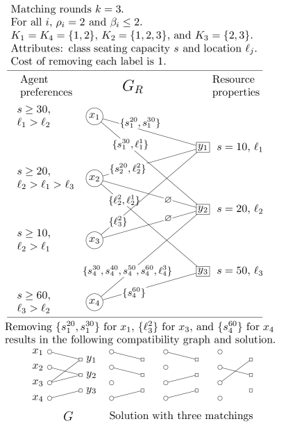
Figure 5: An example of the AG-MRM problem.

A course-classroom example.

This example is motivated by the classroom assignment application considered in this work. See Figure 5. Suppose there are agents (cohorts) who need to be assigned to classrooms on three days ($k=3$) at some specific time such that each agent is assigned a room at least twice ($\forall i,\,\rho_{i}=2$). There are three classrooms. Each agent has preferences regarding the minimum seating capacity of the room, its location, and the rounds in which it would like to be matched. For example, agent $x_{1}$ requires the room to have a capacity (i.e., space) of $\geq 30$, prefers a room in location $\ell_{1}$ over one in $\ell_{2}$, and does not want a room in $\ell_{3}$ (a hard constraint). Also, it wants to be matched in rounds $1$ and $2$. Resource $y_{1}$ has capacity $10$ and is situated in location $\ell_{1}$. The restrictions graph based on agent preferences and resource properties is constructed as follows. To minimize the number of labels, we will assume that each agent can relax its capacity constraint only in steps of $10$. For $x_{1}$ to be compatible with $y_{1}$, it must relax its capacity requirement from $30$ to $10$. To represent this, we introduce two labels $s_{1}^{30}$ and $s_{1}^{20}$ on the edge between $x_{1}$ and $y_{1}$. Removing $s_{1}^{30}$ implies that $x_{1}$ has relaxed its capacity restriction from $30$ to $20$. If a resource is situated in location $\ell_{j}$, then labels corresponding to all locations above $\ell_{j}$ in the agent’s preference order are assigned to the edge. For example, the edge between $x_{2}$ and $y_{3}$ has labels $\ell_{2}^{2}$ and $\ell_{2}^{1}$ as $y_{3}$ belongs to region $\ell_{3}$, which is its least preferred location. The restriction graph for this problem is shown in the middle panel of Figure 5. A solution to AG-MRM in the bottom panels of the figure.

C.2 Generation of restrictions graphs

In the real-world datasets, the agent restrictions are mostly induced by the properties of resources (room size, WiFi connectivity, location, etc.). Three different types of restrictions are considered: binary attributes such as yes/no and present/absent; ordinal attributes such as preferences; and quantitative attributes. The example in Section 3 has binary attributes. We discretize quantitative attributes like capacity by generating labels in steps of some fixed value. Suppose an agent $x$ prefers a resource $y$ of capacity 5, but $y$ has capacity 3, then, we add labels $\ell_{5}$ and $\ell_{4}$ to the restrictions set of edge $\{x,y\}$. To relax the capacity constraint and allow an agent to be matched to a resource of capacity 3, the two labels $\ell_{3}$ and $\ell_{4}$ must be removed. For ordinal attributes we use the following method: suppose $x$ has the following preference order $a>b>c$ for some attribute values $a$, $b$, and $c$ and $y$ has attribute $b$, we add restrictions $\ell_{a}$ to the restrictions set of edge $\{x,y\}$. Relaxing the restriction to accommodate $b$ corresponds to removing $\ell_{a}$. For both real-world datasets, each round corresponds to a day. The cost is assigned as follows: for binary attributes, the cost is 1, while for quantitative and ordinal attributes, the cost on a label depends on the distance from the preferred value: in the above example, the cost $\ell_{5}$ is 1 while the cost of $\ell_{4}$ is 2. The same applies to ordinal attributes.

C.3 An Additional Figure for the Lab-Space dataset

As in Figure 3(d), Figure 6 shows that there is a sharp increase in the number of agents satisfied for a budget of 4. Figure 6 also implies that the performance of PS-AG-MaxSA-MRM is close to that of optimum (given by ILP-AG-MaxSA-MRM). Finally, when budget is high, the fraction of agents satisfied in the latter is reaching $100\%$ while in the former it is at most  $90\%$.

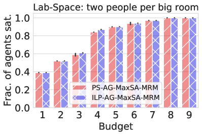
Figure 6: Lab-Space experiment results: Evaluation of the advice generation algorithm for increasing budget when each big room may contain up to two students.

C.4 An Additional Figure for the Course-Classroom dataset

In Figure 7 we demonstrate how critical the current set of resources is for having a satisfactory solution for the  Course-Classroom application. We withheld only a portion of the resources (by sampling) to satisfy the agents’ preferences. The motivation behind this is that some of the university’s classrooms are to be dynamically allocated for some conferences and other events during the year, and the Principal needs to decide in advance what capacity to keep free for such events. The graph shows that with 80% of the resources, it is possible to achieve an average assignment ratio of about  $0.8$.

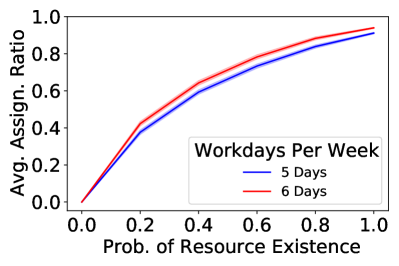
Figure 7: Course-Classroom results. Average assignment ratio when the number of resources is restricted.

C.5 Additional Figures for Synthetic Graphs

To analyze the performance of the algorithms with respect to size of the network, we consider complete bipartite graphs where the number of agents $n$ and resources $m$ are the same. The number of agents (same as resources) is varied from 50 to 200. There are 10 restrictions per agent assigned costs randomly between 1 and 4. For each edge, we randomly assign a restrictions subset of size at most five. For each agent $x_{i}$, the number of rounds $\rho_{i}$ is chosen randomly between $1$ and $5$. To generate $K_{i}$, $\rho_{i}$ rounds are sampled uniformly followed by choosing the remaining rounds with probability $0.5$. The results in Figure 8 show the performance of PS-AG-MaxSA-MRM with respect to ILP-AG-MaxSA-MRM in terms of solution quality and computation time. We note that not only is the solution obtained using the PS-AG-MaxSA-MRM close to the ILP-based algorithm, but it is also orders of magnitude faster.

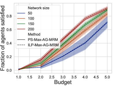
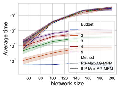
Figure 8: Results for synthetic graphs: Solution quality and computation time.

C.6 Implementation Details

All the software modules used to implement our algorithms and heuristics were written in Python 3.9. Graphs were generated and graph algorithms were implemented using the Networkx package (Hagberg, Swart, and Chult 2008). For local search, we used the simulated annealing implementation by Simple AI (Fisanotti, Carrascosa, and Romero 2012). We use “state” to be a set of relaxations per agent (only the relevant ones as described). Energy is the number of agents satisfied or the number of successful matchings, depends on the specific problem. We use the geometric schedule. By trial and error, we found the best setting of T1 to be 0.99 and T0 to be 100. If the temperature decreased beyond 0.01, we set it to be 0.01. We stopped after 1000 iterations, moved back to the best solution if there was no improvement in 40 iterations and returned the best found solution. We used Gurobi Optimizer (Gurobi Optimization, LLC 2021) for solving the Integer Linear Problems. The advice generation experiments were performed on a Linux machine equipped with two Intel 2.0 GHz Xeon Gold 6138 CPU processors (40 cores and 80 threads in total) and 192 GB of memory. The other experiments, which required fewer resources, were performed using the ’Google Colab’ platform. In all places where random numbers were generated, we used the default seeds provided by python 3.9 and the Linux operating system we used.

Appendix D A General Result on Maximizing Utilitarian Welfare

Theorem D.1.

Suppose the benefit function $\mu_{i}$ of each agent $x_{i}$ is valid and strictly monotone increasing in the number of rounds. Any solution that maximizes the total benefit corresponding to these benefit functions also maximizes the utilitarian welfare, i.e., it maximizes the total number of rounds assigned to the agents.

Proof:  The proof is by contradiction. Suppose $\mathcal{M}^{*}$ is a solution that provides the maximum benefit when each benefit function satisfies the properties mentioned in the theorem. We will show that if there exists a solution $\mathcal{M}$ with number of total assignments greater than that of $\mathcal{M}^{*}$, then, that solution can be modified to a solution $\mathcal{M}^{\prime}$ with benefit $\mathbb{B}(\mathcal{M}^{\prime})>\mathbb{B}(\mathcal{M}^{*})$, contradicting the fact that $\mathcal{M}^{*}$ is an optimal solution.

For each agent $x_{i}$, Let $\gamma_{i}(\mathcal{M})$ be the number of matchings in which $x_{i}$ participates in $\mathcal{M}$.

Steps for creating $\mathcal{M}^{\prime}$ given $\mathcal{M}$ and $\mathcal{M}^{*}$.

• Let $t=0$ and initialize $\mathcal{M}^{\prime}_{t}=\mathcal{M}$.

• while$\big{(}\exists x_{i}$ for which $\gamma_{i}(\mathcal{M}^{*})>\gamma_{i}(\mathcal{M}^{\prime}_{t})\big{)}$:

  • Let $\mathcal{M}^{\prime}_{t+1}=\mathcal{M}^{\prime}_{t}$

  • pick $\gamma_{i}(\mathcal{M}^{*})-\gamma_{i}(\mathcal{M}_{t}^{\prime})$ rounds in which $x_{i}$ participates in $\mathcal{M}^{*}$ but not in $\mathcal{M}_{t}^{\prime}$.

  • In each round, match $x_{i}$ to the same resource it was matched to in $\mathcal{M}^{*}$. If that resource is already matched to another agent in $\mathcal{M}_{t}^{\prime}$, then replace that corresponding edge with the new edge.

  • $t\leftarrow t+1$

• return $\mathcal{M}^{\prime}=\mathcal{M}^{\prime}_{t}$.

Lemma D.2.

In each iteration of the algorithm, the total number of rounds assigned to all agents does not decrease, i.e., the total number of rounds in $\mathcal{M}^{\prime}_{t}$ is at least as large as that in $\mathcal{M}^{\prime}_{t-1}$.

Proof.

In the construction of $\mathcal{M}^{\prime}_{t}$, for every edge added, at most one edge is removed from $\mathcal{M}^{\prime}_{t-1}$. ∎

Lemma D.3.

The algorithm for creating $\mathcal{M}^{\prime}$ terminates.

Proof.

First, in each iteration, the algorithm adds at least one edge from $\mathcal{M}^{*}$ to $\mathcal{M}^{\prime}$. Second, once an edge is added it will never be removed since each edge that is added belong to one of the matchings in $\mathcal{M}^{*}$. ∎

Lemma D.4.

For all benefit functions that fulfil the conditions of the theorem, $\mathbb{B}(\mathcal{M}^{\prime})>\mathbb{B}(\mathcal{M}^{*})$.

Proof.

As before, we use $\gamma_{i}(\mathcal{M})$ to denote the number of rounds assigned to $x_{i}$ in solution $\mathcal{M}$. Note that for each $i$, $\gamma_{i}(\mathcal{M}^{\prime})>\gamma_{i}(\mathcal{M}^{*})$. By the contradiction assumption, the number of assignments in $\mathcal{M}$ is grater than that of $\mathcal{M}^{*}$ and therefore initially in $\mathcal{M}^{\prime}$. During the construction, the number of assignments does not decrease and therefore there exists at least one $i$ for which $\gamma_{i}(\mathcal{M}^{\prime})>\gamma_{i}(\mathcal{M}^{*})$. Since the benefit function, $\mu_{i}$ is increasing for all $i$, it follows that $\mathbb{B}(\mathcal{M}^{\prime})>\mathbb{B}(\mathcal{M}^{*})$. ∎

The last lemma above shows that $\mathbb{B}(\mathcal{M}^{\prime})>\mathbb{B}(\mathcal{M}^{*})$. This contradicts the optimality of $\mathcal{M}^{*}$ and the theorem follows. $\Box$

References

- Aarts and Korst (1989) Aarts, E.; and Korst, J. 1989. Simulated Annealing and Boltzmann Machines: A Stochastic Approach to Combinatorial Optimization and Neural Computing. New York, NY: Wiley.
- Anshelevich et al. (2013) Anshelevich, E.; Chhabra, M.; Das, S.; and Gerrior, M. 2013. On the social welfare of mechanisms for repeated batch matching. In AAAI.
- Babaei, Karimpour, and Hadidi (2015) Babaei, H.; Karimpour, J.; and Hadidi, A. 2015. A survey of approaches for university course timetabling problem. Computers & Industrial Engineering, 86: 43–59.
- Cai and Khan (2010) Cai, H.; and Khan, S. 2010. The common first year studio in a hot-desking age: An explorative study on the studio environment and learning. J. for Education in the Built Environment, 5(2): 39–64.
- Caragiannis and Narang (2022) Caragiannis, I.; and Narang, S. 2022. Repeatedly Matching Items to Agents Fairly and Efficiently. arXiv preprint arXiv:2207.01589.
- Chevaleyre et al. (2006) Chevaleyre, Y.; Dunne, P. E.; Endriss, U.; Lang, J.; Lemaître, M.; Maudet, N.; Padget, J. A.; Phelps, S.; Rodríguez-Aguilar, J. A.; and Sousa, P. 2006. Issues in Multiagent Resource Allocation. Informatica (Slovenia), 30(1): 3–31.
- Cormen et al. (2009) Cormen, T. H.; Leiserson, C. E.; Rivest, R. L.; and Stein, C. 2009. Introduction to Algorithms. Cambridge, MA: MIT Press and McGraw-Hill.
- District Management Group (2020) District Management Group. 2020. COVID-19: Creating Elementary School Schedules to Support Social Distancing DMGroup Research Briefs. https://f.hubspotusercontent00.net/hubfs/3412255/Resources“%20Page“%20Files“%20-“%20Public/DMGroup-School-Restart-Research-Brief-Elementary-School-Schedules-and-Social-Distancing˙2020-7.pdf.
- Dolgov and Durfee (2006) Dolgov, D. A.; and Durfee, E. H. 2006. Resource Allocation Among Agents with MDP-Induced Preferences. J. Artif. Intell. Res., 27: 505–549.
- Eley (2006) Eley, M. 2006. Ant algorithms for the exam timetabling problem. In International Conference on the Practice and Theory of Automated Timetabling, 364–382. Springer.
- Enriching Students (2020) Enriching Students. 2020. School Schedules During COVID-19–A Guide to assist schools. https://www.enrichingstudents.com/school-schedules-during-covid-19/.
- Felfernig et al. (2011) Felfernig, A.; Friedrich, G.; Jannach, D.; and Zanker, M. 2011. Developing Constraint-based Recommenders. In Recommender Systems Handbook, 187–215. Springer.
- Fisanotti, Carrascosa, and Romero (2012) Fisanotti, J. P.; Carrascosa, R.; and Romero, S. 2012. Simple AI.
- Fonseca, Santos, and Carrano (2016) Fonseca, G. H.; Santos, H. G.; and Carrano, E. G. 2016. Integrating matheuristics and metaheuristics for timetabling. Computers & Operations Research, 74: 108–117.
- Garey and Johnson (1979) Garey, M. R.; and Johnson, D. S. 1979. Computers and Intractability: A Guide to the Theory of NP-completeness. W. H. Freeman and Co.
- Gilbert (2018) Gilbert, F. 2018. A Guide to Sharing Farm Equipment. https://projects.sare.org/wp-content/uploads/Sharing-Guide-2018-“˙-Web.pdf.
- Gollapudi, Kollias, and Plaut (2020) Gollapudi, S.; Kollias, K.; and Plaut, B. 2020. Almost envy-free repeated matching in two-sided markets. In Int. Conf. on Web and Internet Economics.
- Gorodetski, Karsaev, and Konushy (2003) Gorodetski, V. I.; Karsaev, O.; and Konushy, V. 2003. Multi-agent System for Resource Allocation and Scheduling. In Proc. CEEMAS, 236–246.
- Gurobi Optimization, LLC (2021) Gurobi Optimization, LLC. 2021. Gurobi Optimizer Reference Manual.
- Hagberg, Swart, and Chult (2008) Hagberg, A.; Swart, P.; and Chult, D. S. 2008. Exploring network structure, dynamics, and function using NetworkX. Technical report, Los Alamos National Lab.(LANL), Los Alamos, NM (United States).
- Karamanis, Anastasiadis, and Angeloudis (2020) Karamanis, R.; Anastasiadis, E.; and Angeloudis, M., P. Stettler. 2020. Assignment and pricing of shared rides in ride-sourcing using combinatorial double auctions. IITS.
- Kucharski and Cats (2020) Kucharski, R.; and Cats, O. 2020. Exact matching of attractive shared rides (ExMAS) for system-wide strategic evaluations. Transportation Research Part B: Methodological, 139: 285–310.
- Leite, Melício, and Rosa (2019) Leite, N.; Melício, F.; and Rosa, A. C. 2019. A fast simulated annealing algorithm for the examination timetabling problem. Expert Systems with Applications, 122: 137–151.
- Liu (2020) Liu, C. 2020. Stability in repeated matching markets. arXiv preprint arXiv:2007.03794.
- Nguyen, Roos, and Rothe (2013) Nguyen, T. T.; Roos, M.; and Rothe, J. 2013. A survey of approximability and inapproximability results for social welfare optimization in multiagent resource allocation. AMAI, 68(1-3): 65–90.
- Parker (2020) Parker, L. D. 2020. The COVID-19 office in transition: cost, efficiency and the social responsibility business case. Accounting, Auditing & Accountability J.
- Phillips et al. (2015) Phillips, A. E.; Waterer, H.; Ehrgott, M.; and Ryan, D. M. 2015. Integer programming methods for large-scale practical classroom assignment problems. Computers & Operations Research, 53: 42–53.
- Rakhra and Singh (2020) Rakhra, M.; and Singh, R. 2020. Internet Based Resource Sharing Platform development For Agriculture Machinery and Tools in Punjab, India. In Proc. 8th International Conference on Reliability, Infocom Technologies and Optimization (Trends and Future Directions) (ICRITO), 636–642.
- Rawls (1999) Rawls, J. 1999. A Theory of Justice. Harvard University Press.
- Stark (2020) Stark, O. 2020. An economics-based rationale for the Rawlsian social welfare program. University of Tübingen Working Papers in Business and Economics, No. 137.
- Sühr et al. (2019) Sühr, T.; Biega, A. J.; Zehlike, M.; Gummadi, K. P.; and Chakraborty, A. 2019. Two-sided fairness for repeated matchings in two-sided markets: A case study of a ride-hailing platform. In Proceedings of the 25th ACM SIGKDD International Conference on Knowledge Discovery & Data Mining, 3082–3092.
- Tan et al. (2021) Tan, J. S.; Goh, S. L.; Kendall, G.; and Sabar, N. R. 2021. A survey of the state-of-the-art of optimisation methodologies in school timetabling problems. Expert Systems with Applications, 165: 113943.
- Trabelsi et al. (2022a) Trabelsi, Y.; Adiga, A.; Kraus, S.; and Ravi, S. 2022a. Maximizing Resource Allocation Likelihood with Minimum Compromise. In Proceedings of the 21st International Conference on Autonomous Agents and Multiagent Systems, 1738–1740.
- Trabelsi et al. (2022b) Trabelsi, Y.; Adiga, A.; Kraus, S.; and Ravi, S. 2022b. Resource Allocation to Agents with Restrictions: Maximizing Likelihood with Minimum Compromise. In Proc. European Conference on Multi-Agent Systems (EUMAS).
- Varone and Beffa (2019) Varone, S.; and Beffa, C. 2019. Dataset on a problem of assigning activities to children, with various optimization constraints. Data in brief, 25: 104168.
- Viner (1949) Viner, J. 1949. Bentham and JS Mill: The utilitarian background. The American Economic Review, 39(2): 360–382.
- Wong (2021) Wong, M. 2021. Self-scheduler for dental students booking consultations with faculty during the COVID-19 pandemic. Journal of Dental Education.
- Zahedi, Sengupta, and Kambhampati (2020) Zahedi, Z.; Sengupta, S.; and Kambhampati, S. 2020. ’Why not give this work to them?’ Explaining AI-Moderated Task-Allocation Outcomes using Negotiation Trees. CoRR, abs/2002.01640.
- Zanker, Jessenitschnig, and Schmid (2010) Zanker, M.; Jessenitschnig, M.; and Schmid, W. 2010. Preference reasoning with soft constraints in constraint-based recommender systems. Constraints An Int. J., 15(4): 574–595.
- Zhou and Han (2019) Zhou, W.; and Han, W. 2019. Personalized Recommendation via User Preference Matching. Information Processing and Management, 56(3): 955–968.