METAHEURISTIC APPROACH TO SOLVE PORTFOLIO SELECTION PROBLEM

Abstract

In this paper, a heuristic method based on Tabu Search and TokenRing Search is being used in order to solve the Portfolio Optimization Problem. The seminal mean-variance model of Markowitz is being considered with the addition of cardinality and quantity constraints to better capture the dynamics of the trading procedure, the model becomes an NP-hard problem that can not be solved using an exact method. The combination of three different neighborhood relations is being explored with Tabu Search. In addition, a new constructive method for the initial solution is proposed. Finally, I show how the proposed techniques perform on public benchmarks.

I Introduction

Financial markets are at the heart of the modern economy and provide an avenue for selling and purchasing assets such as bonds, stocks, foreign exchange, and derivatives. The prime objective of any investor when investing in any of these markets is to minimize the risk involved in the trading process and maximize the profits generated, this objective can be met by diversifying the amount of money to be invested (Capital) among a set of available assets. Each one of the different ways to choose assets and diversify the capital between them is called a portfolio(or Securities) and the problem of finding this optimal portfolio that maximizes profits and minimizes risk is called Portfolio Optimization Problem (POP) or Portfolio Selection Problem. In his seminal work, Markowitz [1] proposed the Mean-Variance model to solve the portfolio optimization problem, which assumes that the risk of a particular portfolio can be minimized by minimizing the co-variance between the portfolio assets, i.e., minimizing the chance of loss by choosing assets that do not tend to move together (low co-variance), so if one asset’s price is going down the other asset will still have a chance to make up for the losses. Despite the pioneer model of Markowitz, it does not reflect the real-life trading procedure by lacking cardinality constraints that set a limit to the number of assets allowed in a portfolio as well as lacking any bounding constraints that set limits to the amount of money allowed to be invested in each asset.
In this paper, an extension of Markowitz [1] model is being considered, in which cardinality constraints and quantity constraints are imposed to make it more adherent to real-world trading mechanisms. The addition of these constraints will turn the model from Quadratic Programming (QP) problem to a Mixed Integer Quadratic Programming (MIQP) problem, which is an NP-Hard problem that can not be solved using an exact method, therefore a Metaheuristic approach is needed.
The use of local search techniques for the POP has been proposed by Chang et al. (2000).[2]. Here, I investigate the possible improvement of their Tabu Search (TS) technique by first, proposing an alternative of Initial Solution generation (Constructive heuristics) based on the Sharp Ration rather than randomly assigning the initial solution. Second, I introduce an additional move to diversify the search space and escape the local optima also instead of using a fixed step size, different step sizes are being considered, and finally, I investigate the application of the Token-Ring method with the Tabu search algorithm to implement Multi-Neighborhood Search. The proposed techniques are tested on the benchmarks proposed by Chang et al. (2000).[2] which represent real stock markets.

II Related Work

Chang et al. [2] used three different metaheuristic approaches (Genetic Algorithm, Simulated Annealing, and Tabu Search) to solve a multi-objective portfolio optimization problem with cardinality & quantity constraints. They reported that no individual heuristic was found to be dominating across five data sets. Schaerf et al. [3] explored the use of Tabu Search on single-objective constrained POP, and also proposed new algorithms that combine different neighborhood relations. They implemented several token-ring procedures in a way to diversify and intensify the search space and they concluded that TS is the most promising heuristic to solve POP. In an attempt of making the mean-variance model more realistic, Soleimani et al.[4] introduced sector capitalization as an additional constraint to reduce investment risk, they used GA and compared the results of a small instance problem to the results found by LINGO (which can generate global optima for small problems) and reported that the difference between LINGO’s global optimum and GA’s best objective is just 2.9%. By combining local search techniques (SD & FD) and exact mathematical programming (Quadratic programming solver) Gaspero et al. [5] proposed a hybrid local search algorithm, according to their results, the developed solver finds the optimal solution in several instances and is at least comparable to other state-of-the-art methods from the others.
Surveying the techniques used in literature ([2], [3], [4], [7], [8], [9]) to solve the constrained portfolio optimization problem reveals that Genetic Algorithm is the most used technique to solve the problem, where a couple of studies ([3] ,[4]) considered using Tabu search.

III Portfolio Optimization Problem

In this section, the portfolio selection (or optimization) problem is introduced in stages. The unconstrained Markowitz model is represented first in Section III-A. Subsequently, I introduce the specific constraints of the formulation considered in this study in Section III-B. Finally, the Efficient Frontier is explained in Section III-C.

III-A Unconstrained Markowitz model

Given a set of n available assets, $A=\{a_{1},a_{2},...,a_{n}\}$, let $\mu_{i}$ be the expected return (increase in asset price) for asset $a_{i}$ and $x_{i}$ the portion of the capital invested in asset $a_{i}$, and each pair of assets $(a_{i},a_{j})$ has a real value of co-variance $\sigma_{ij}$. Let $\mu_{p}$ represent the desired return from the portfolio, thus the formulation of the unconstrained problem is given as:

$$min\sum_{i=1}^{n}\sum_{j=1}^{n}x_{i}x_{j}\sigma_{ij}$$ (1)

$$S.t.\,\,\,\,\,\,\,\,\,\,\,\,\,\,\,\,\,\,\,\,\,\,\,\,\,\,\,\,\,\,\,\,\,\,\,\,\,\,\,\,\,\,\,\,\,\,\,\,\,\,\,\,\,\,\,\,\,\,\,\,\,\,\,\,\,\,\,\,\,$$

$$\sum_{i=1}^{n}\mu_{i}x_{i}\geq\mu_{p}$$ (2)

$$\sum_{i=1}^{n}x_{i}=1$$ (3)

$$0\leq x_{i}\leq 1\,\,\,\,i=1,2,...,n$$ (4)

Eq. (1) minimizes the total variance (risk) associated with the portfolio, Eq. (2) ensures that the portfolio has an expected return of or bigger than $\mu_{p}$. Eq. (3) ensures that 100% of the capital is being invested and short-selling is not feasible.

III-B Constrained Markowitz model

While the previous single-objective model considers only minimal risk for a given expected return it’s desirable to also seek a maximum return for a given expected level of risk, this can be achieved by subsuming the expected return constraint into the objective function via a weighting approach which yields a profitable algorithmic approach. The objective function in Eq.(1) will become Eq.(5), where $\lambda$ represents the risk aversion of the investor, when set to 0 the investor is taking high risk in order to maximize the profits, if 1, the investor is not willing to take any risk but profits will not be necessarily maximized (Eq.(10))
The cardinality constraint will determine the number of assets k the portfolio must include. A binary variable $z_{i}$ is introduced to denote whether an asset is being selected or not. Eq.(7) & Eq.(11). Whereas quantity constraint will set boundaries for the weights (proportions) of included assets by specifying a lower ($\epsilon$) and upper ($\delta$) bounds allowed for the allocated proportions to each asset in the portfolio, Eq.(8).

$$min\,\,\,\lambda[\sum_{i=1}^{n}\sum_{j=1}^{n}x_{i}x_{j}\sigma_{ij}]-(1-\lambda)\sum_{i=1}^{n}\mu_{i}x_{i}$$ (5)

$$\sum_{i=1}^{n}x_{i}=1$$ (6)

$$\sum_{i=1}^{n}z_{i}=K$$ (7)

$$\epsilon z_{i}\leq x_{i}\leq\delta z_{i}\,\,\,\,\,\,i=1,2,...,n$$ (8)

$$0\leq x_{i}\leq 1\,\,\,\,\,\ i=1,2,...,n$$ (9)

$$0\leq\lambda\leq 1$$ (10)

$$z_{i}=\begin{cases}1,&\text{if asset i is held}\\ 0,&\text{otherwise}\end{cases}$$ (11)

$$z_{i}\in\{1,0\},\,\,\,\,\,\ i=1,2,...,n$$ (12)

Where:

• n: number of stocks in the dataset.

• $\lambda$ : The risk aversion of the investor

• $x_{i}$ : Proportion of capital invested in asset i

• $\sigma_{ij}$ : The co-variance between asset i and j

• $\mu_{i}$ : The expected return of the asset i

• K: the number of assets in the portfolio

• $\epsilon$ : The minimum proportion invested in asset

• $\delta$ : The maximum proportion invested in asset

This formulation is a multi-objective mixed quadratic and integer programming problem for which exact methods do not exist.

III-C Efficient Frontier

Due to the fact that the problem in this study is multi-objective optimization problem and usually has several different optimal solutions, it’s useful to approach the problem as Pareto Optimality Problem [10], that is by solving the QP in Section III-A for varying values of $\mu_{p}$ (the desired return from the portfolio) we can trace a non-decreasing curve that represents the set of Pareto-optimal (non-dominated) portfolios, i.e., gives for each expected return the minimum associated risk. We call this curve The Unconstrained Efficient Frontier (UEF), Fig.1 shows the UEF for the smallest benchmark problem in [2], which has been computed taking 2000 different values of $\mu_{p}$ and solving the unconstrained POP. In a similar way, the UEF for each data set in the benchmark is shown in Table III.

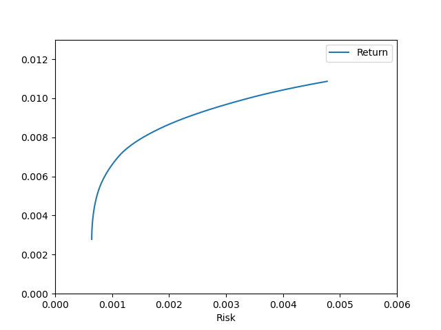
Figure 1: Unconstrained Efficient Frontier corresponding to the smallest benchmark problem. (UEF of Hang Seng)

Given that the constraint problem has never been solved exactly (Eqs.(5)-(12)), the quality of the heuristic method will be measured in average percentage loss w.r.t. the UEF. i.e., taking the sets of Pareto optimal portfolios obtained by solving the constrained POP using the proposed heuristic approach we can trace out the heuristic efficient frontier and compare it to the UEF (More is SectionVI)

IV Portfolio Optimization by Tabu Search

For any local search method such as Tabu Search (TS), there are essential components we need to define, Initial Solution, Neighborhood Structures, and Search Space. In this section, these components will be described in addition to the TS algorithm parameters used in this study.

IV-A Search Space and Neighborhood Structures

In POP, the solution (portfolio) consists of two parts, the first part is the set of assets chosen from the pool of available ones, and the second part is the capital proportions allocated to each chosen asset. Hence, the solution will be represented as two sequences, $L={[a_{1},...,a_{n}]}$ and $S={[x_{1},...,x_{n}]}$ such that $a_{i}$ is an asset in the solution (portfolio) and $x_{i}$ is the capital fraction invested in asset $a_{i}$, where the length of L satisfies Eq.(7) and S satisfies Eq.(6), Eq.(8) and Eq.(9).
As we are trying to optimize a continuous variable (capital fractions), the neighborhood generation is defined over the step of the move performed on the current solution. Given a step size q which is a real-value parameter we can define two moves to explore the search space, Increase_move and Decrease_move. The idea is to increase and decrease each of the asset weights in the solution in order to find the optimal ones. To illustrate the aforementioned neighborhood relation further suppose that the current solution is $L=[{2,8}]$ and $S={[0.65,0.35]}$, the neighborhood solutions following the Increase_move with step size q = 0,8 would be $S1={[(1+0.8)\times 0.65,0.35]}$ and $S2={[0.65,(1+0.8)\times 0.35]}$ and the same for the Decrease_move with replacing (1+ 0.8) by (1- 0.8).

• Increase_move (Solution, i, q):

  • Description: Increases the weight of asset i in Solution. The number of neighbors generated equals to the number of assets k in the solution.

  • Effects: $x_{i}=x_{i}\times(1+q)$

• Decrease_move (Solution, i, q):

  • Description: Decreases the weight of asset i in the Solution. The number of neighbors generated equals to the number of assets k in the solution.

  • Effects: $x_{i}=x_{i}\times(1-q)$, if $x_{i}<\epsilon$ replace asset i with a randomly chosen asset j, not in the solution.

Notice in the example shown above, the S1 neighbor solution becomes $S1={[1.17,0.35]}$ which violates the constraints imposed. To ensure that all solutions in the searching space satisfy the imposed constraints (all weights sum up to one and satisfy the upper and lower bounds), Rescale (see Algorithm 1) algorithm is introduced [2].

In addition to the Increase_move and Decrease_move, a third move is added to diversify the search which is the Swap_move, this move swaps the asset with the lowest weight in the solution by an asset, not in the solution.

• Swap_move (Solution, j):

  • Description: Swaps asset i which has the lowest weight in Solution by asset j, not in Solution. The number of neighbors generated equals (number of assets available N - number of assets k in the solution)

  • Effects: Swap(i,j), $i\in Solution,j\notin Solution$ keep the same weights

Input: Solution

Output: Solution which satisfies cardinality and quantity constraints

// K is #assets in Solution

1 free_proportion = $1-(K\times\epsilon)$

2 weight_sum = $\sum_{i\in Solution}x_{i}$

// Fixing weights to add up to 1 and no weight is < $\epsilon$:

3 for Each $x_{i}$ in Solution do

4       $x_{i}=\epsilon+(x_{i}/weight\_sum)\times free\_proportion$

// No weight is > $\delta$:

5 R = Assets in Solution with weights $>\delta$

6 if R not empty then

7      L = $\sum_{i\in Solution-R}x_{i}$

8       free_proportion = $1-(K\times\epsilon+length(R)\times\delta)$

9       for Each $x_{i}$ in Solution do

10             if $x_{i}<\delta$ then

11                  $x_{i}=\epsilon+(x_{i}/L)\times free\_proportion$

12            else

13                  $x_{i}=\delta$

14            

15      

16return Solution

Algorithm 1 Rescale

IV-B Initial Solution Construction

In the literature [2], the initial feasible solution is selected as the best among randomly generated portfolios with K assets. In this project, I propose a Greedy approach (similar to Fractional Knapsack Problem) based on Sharpe Ration[12], which is basically the ratio of the expected return of an asset to its standard deviation. (See Algorithm 2). To illustrate the effectiveness of the proposed greedy algorithm to find an initial solution, I solve a small problem (toy problem) that had been solved using the exact method, the General Algebraic Modeling System (GAMS) in [13]. As the problem in [13] is an unconstrained Portfolio Optimization Problem (POP), the constraints are relaxed in our model to match with the one solved by [13], Lambda = 1, Capital = 1000, k=3, epsilon = 0.0, delta = 1, T= 10000, where T is the number of iterations to generate random weights and evaluate them, so by increasing T we might get a better solution but with computation trade-off. The obtained results, i.e., proportions of the capital to be invested in each stock, are very close to the ones found by the exact method, which is a good indication of the efficiency of the proposed approach. Solution found by GAMS : {0.497 IBM, 0.0 WMT, 0.502 SEHI}, Solution found by the Greed algorithm : {0.442 IBM, 0.1036 WMT, 0.454 SEHI}(See Code & Notebook here)

Input: Expected returns, Standard deviations, Number of iterations to perform(T)

Output: {stock_1: $x_{1}$, stock_2: $x_{2}$,…, stock_n: $x_{n}$}

L = []

  // Starting with empty set of assets

S=[]

  // Starting with empty set of fractions

T = Integer

  // Number of specified Iterations

1 Best_solution = {}

V = Infinite

  // Best value found for the objective function

2 for Each available asset do

3       Calculate Sharpe_ratio = Asset Return / Standard Deviation

4Rank available assets based on their Sharpe_ratio in a descending order

Add the first K assets to L

  // Constraint in Eq.(7)

5 for t=1 to T do

       S = {}

        // Current solution in the iteration

       f = 0

        // Current value for the objective function

6      

7      for Each asset in L do

             // Constraint in Eq.(8) & Eq.(9)

8             $x_{i}$ = randomly assign a value between $\epsilon$ and $\delta$

      Renormalize weights in S to add up to one

        // Constraint in Eq.(6)

9       if $f<V$ & length(S) = k then

10            Update the best solution

11             V = f

12             Best_solution = S

13      

14return L, S

Algorithm 2 Initial Solution

IV-C Tabu Search Parameters

The parameters of TS are tuned using the Grid Search technique, i.e., testing different combinations of the parameters and choosing the best-performing one.

• Tabu List: For each neighborhood relation a tabu list is created. Tabu tenure is set to 3 throughout the whole algorithm (static) for Increase_move and Decrease_move, whereas for Swap_move the tabu tenure is 20 due to the fact that this move contributes to the stability of the search.

• Tabu Attribute: Because TS aggressively selects the best admissible solution from the neighborhood space, moves are isolated and updated in short-term memory, which records the increase/decrease of the move value for each solution in the neighborhood. The tabu attribute of Increase_move and Decrease_move is the asset that has been increased/decreased. Swap_move is the asset that has been added by the move to the solution. For example, [asset5: {Increase: 0, Decrease: 3, Swap: 20}] which means that asset5 is tabu to be Decrease for the next three iterations but it’s not for Increasing move, and it’s tabu to be removed (swapped) if it has the lowest weight in solution for the 20 next iterations.

• Aspiration Criteria: If the current move is tabu but delivers a better solution than the best found one, its tabu statute is overridden.

• Termination Condition: When a solution that improves the Best (the incumbent) solution cannot be obtained in 200 consecutive iterations.

V Token Ring Search

The token-ring search is a sequential solving strategy for combining different neighborhood functions. Given an initial state and a set of algorithms or what we call runners, the token-ring search makes circularly a run of each runner, always starting from the best solution found by the previous one. The effectiveness of the token-ring search for two runners has been stressed by several authors [11].

V-A t1 Runner

Given a step size q, the t1 runner uses the TS algorithm described in Section IV to search the space for the local optima solution. That is, given an initial solution $S_{0}$, t1 will iterate to update the current and best solutions, by choosing a non-tabu move or Best-improving move from the Neighborhood Union of the three neighborhood relations applied on the current solution. Algorithm 3 shows the details of the t1-TS runner.

Input: Initial_Solution, q

Output: local optima solution found using step size q

1 Best_Solution = Initial_Solution

2 Current_Solution = Initial_Solution

// Generate neighborhood solutions from the Current_Solution:

3 Neighbors_Solutions = []

4 for asset i in Current_Solution do

5      Add Increase_move (Current_Solution, i, q) & Decrease_move ((Current_Solution, i, q) to Neighbors_Solutions

6for asset j not in Current_Solution do

7      Add Swap_move (Current_Solution, j) to Neighbors_Solutions

8Select admissible move from Neighbors_Solutions: Select the non-tabu improving or least Improving move. Override tabu statues if the move meet the aspiration criteria.

9 Update Current_Solution & Best_Solution

10 Check Termination:

11 if No Best_Solution found in 200 consecutive iteration then

12      Return Best_Solution

13else

14      Go to step 3

15

Algorithm 3 t1_TS

V-B t2 Runner

In the t2 runner, the step size q is defined. Step Size q starts with a big value (q = 5) and decreases by 0.2 for each run of the t1 runner until it reaches 0.2. By starting with big steps we guarantee diversification by making big moves and small steps provide intensification with small moves. Here, I define one run of the t2 runner as a complete iteration over all step sizes using the t1 runner. t2 runner stops when no improving solution is found by the current run (See Algorithm 4). t1_TS always starts from the best solution found by the previous one.

Input: Initial_Solution

Output: Best Solution

1 Initialize: step_size_list = $[q_{1}=5,q_{2}=4.8,...,q_{n}=0.2]$

2 Initial_Solution = Initial Solution Algorithm

Next_Solution=t1_TS(Initial_Solution, $q_{0}=5.2$)

  // 3

for step $q_{i}$ in step_size_list

  // One r2 run

3 do

4      Reset tabu time of all moves

5       Next_Solution = t1_TS (Next_Solution , $q_{i}$)

6if Improved solution found by any step_size in 4 then

      Go to 4

        // another t2 run

7      

8

9else

      // Final Soluiton

10      Stop & return Next_Solution

11

Algorithm 4 t2

VI Computational Experiments

VI-A Benchmarks and experimental setting

In this section, the proposed approach in this study is being used to solve the Constrained Model described in SectionIII-B. I have done all the computational experiments with five sets of benchmark data that have been already used in [2]. These data correspond to weekly prices from March 1992 to September 1997 and they come from the indices: Hang Seng in Hong Kong, DAX_100 in Germany, FTSE_100 in the UK, S&P_100 in the USA, and Nikke_225 in Japan. The number of assets varies within each data set: 31, 85, 89, 98, and 225 assets, respectively. Data Source
All the results presented here have been computed as in [2], using the values $K=10,\epsilon=0.01and\delta=1$ for the problem formulation, and the values $\Delta\lambda=0.02$ for the implementation. So the method is implemented with 51 different values for the risk aversion parameter $\lambda$. As a result for each benchmark data we have 51 optimal solutions (Portfolios), and each has the best objective function value found by the proposed heuristic for the weighting parameter $\lambda$. From these obtained portfolios (solutions) we can trace back the Constrained Efficient Frontier (CEF) by calculating the Return and Variance of return (Risk) of each portfolio. Fig 2 shows the CEF for the smallest benchmark data, where 51 points are plotted, and each point represents a solution (Portfolio) with (x=Risk,y = Return). Similarly, Table III shows the UEF for each data set in the benchmark.

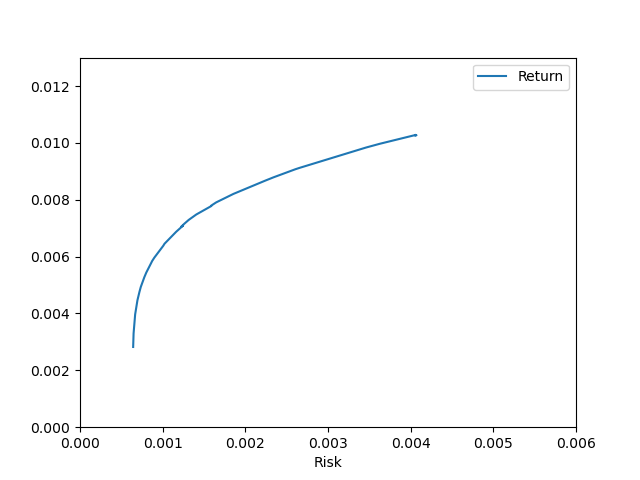
Figure 2: Constrained Efficient Frontier corresponding to the smallest benchmark problem. (UEF of Hang Seng)

TABLE I: Comparison of the proposed method performance with benchmark TS algorithm

Index	Assets		TS&TokenRing	TS In Ref[2]
Hang Seng	31	Median percentage error Mean percentage error Time (s)	1.812 2.2656 1154.3	1.2181 1.1217 74
DAX	85	Median percentage error Mean percentage error Time (s)	4.21 4.035 2873	2.6380 3.3049 199
FTSE	89	Median percentage error Mean percentage error Time (s)	1.2406 1.2959 2919	1.0841 1.6080 246
S&P	98	Median percentage error Mean percentage error Time (s)	2.3630 2.5068 3107	1.2882 3.3092 225
Nikkei	225	Median percentage error Mean percentage error Time (s)	1.34635 1.21220 5866.2	0.6093 0.8975 545

VI-B Percentage Deviation Calculation

To measure and quantify the quality of the solutions obtained, hence the performance of the proposed method, the percentage deviation (distance) of each portfolio from the (linearly interpolated) Unconstrained Efficient Frontier (UEF) is computed as following:
Let the pair $(v_{i},r_{i})$ represent the variance and mean the return of a point in the CEF (solution found by the proposed method). Let also $(\hat{v_{i}},\hat{r_{i}})$ represent the variance and mean the return of a point in the UEF. We can find $v_{j}$ and $v_{k}$ which brackets $v_{i}$ on the UEF as, $v_{j}=\min[\hat{v_{i}}|\hat{v_{i}}\geq v_{i}]$ and $v_{k}=\max[\hat{v_{i}}|\hat{v_{i}}\leq v_{i}]$ and by simple geometry we can calculate $\hat{\hat{r_{i}}}$ which is the value associated with the x-direction linear interpolated point with $\hat{v_{i}}=v_{i}$ on the UEF. $\hat{\hat{r_{i}}}=r_{k}+(r_{j}-r_{k})[(r_{i}-r_{k})/(r_{j}-r_{k})]$ . From $\hat{\hat{r_{i}}}$ we can calculate convenient percentage deviation error of the solution as $\varphi_{i}=|100\times(r_{i}-\hat{\hat{r_{i}}})/\hat{\hat{r_{i}}}|$. The percentage deviation error associated with y-direction is calculated in the same way but with keeping the Return $\hat{r_{i}}$ fixed instead of $\hat{v_{i}}$. The percentage deviation error measure of solution $(v_{i},r_{i})$ is the minimum of the x-direction, and y-direction percentage deviations. Finally the Median percentage error and Mean percentage error of the 51 solutions found by the proposed method are reported and compared with reference [2] for each data set.

VI-C Results & Conclusion

The results for the proposed heuristic algorithm (Tabu Search with Token-Ring technique) with the number of assets in the portfolio K = 10, a minimum proportion of any asset that must be held (if any is held) $\epsilon=0.01$ and maximum proportion that can be held of any asset (if any is held) $\delta=1$ are shown in Table I.
The results show that the proposed method’s performance is very close to the benchmark approach. For the problems with assets = 98 and 89, the proposed method surpasses the benchmark results in the Mean percentage error, whereas for the rest of the data sets, it delivers sub-optimal results in comparison to the benchmark.
The major drawback of the proposed method in this study is the computation time which was significantly higher than the benchmark as shown in Table I. In conclusion, the proposed method of combining the Token Ring technique with three neighborhood relations failed to surpass the benchmark for some data instances and successfully outperformed it for other data instances. To better analyze the performance of the proposed method, the average error in the first objective (Variance return) and the average error in the second objective (Return) is being reported in Table II. Here, The variance of return (Risk) error for any heuristic point $(v_{i},r_{i})$ is computed as the value $100\times(\hat{v_{i}}-v_{i})/\hat{v_{i}}$, where $\hat{v_{i}}$ is the corresponding to Risk with keeping Return $r_{i}$ fixed according to the linear interpolation in the UEF. The average value of all the errors for the points in heuristic CEF gives us the variance of return error shown in Table II. Similarly, the average Return error is calculated. The analysis indicates that the studied method is performing well for the second objective (Return) and relatively poor with the first objective (Risk), that is for small values of lambda (giving more weight to the second objective) the method performs well, i.e., the method is performing well if we are considering portfolios with high return and small risk.

TABLE II: Comparison between the errors of the first objective and second objectoive

Index	Assets		TS&TokenRing
Hang Seng	31	First Obj (Risk) error Second Obj (Return) error	7.0405 2.4751
DAX	85	First Obj (Risk) error Second Obj (Return) error	49.7685 1.4008
FTSE	89	First Obj (Risk) error Second Obj (Return) error	6.0545 1.8224
S&P	98	First Obj (Risk) error Second Obj (Return) error	20.2107 3.5328
Nikkei	225	First Obj (Risk) error Second Obj (Return) error	9.221 2.2761

TABLE III: The Unconstrained Efficient Frontier (UEF) and the Constrained Efficient Frontier (CEF) of each data set. The Return (second obj) is represented on the y-axis, whereas the Risk (first obj) is represented on the x-axis

o X[c]X[c]

Figure 3: UEF of DAX

Figure 4: CEF of DAX

Figure 5: UEF of FTSE

Figure 6: CEF of FTSE

Figure 7: UEF of S&P

Figure 8: CEF of S&P

Figure 9: UEF of Nikkei

Figure 10: CEF of Nikkei

References

- [1] Markowitz, H., 1952. Portfolio Selection. The Journal of Finance, 7(1), p.77.
- [2] Chang T-J, Meade N, Beasley JE, Sharaiha YM. Heuristics for cardinality-constrained portfolio optimization. Comput Oper Res 2000;27(13):1271–302.
- [3] Schaerf A. Local search techniques for constrained portfolio selection problems.Comput Econ 2002;20(3):177–90. 0104017
- [4] Soleimani H, Golmakani HR, Salimi MH. Markowitz-based portfolio selection with minimum transaction lots, cardinality constraints and regarding sector capitalization using genetic algorithm. Expert Syst Appl 2009;36(3):5058–63.
- [5] Gaspero LD, Tollo GD, Roli A, Schaerf A. Hybrid metaheuristics for constrained portfolio selection problems. Quant Finance 2011;11(10):1473–87.
- [6] J.-S. Chen, J.-L. Hou, S.-M. Wu, and Y.-W. Chang-Chien, “Constructing investment strategy portfolios by combination genetic algorithms,”Expert Systems with Applications, vol. 36, no. 2, Part 2, pp. 3824 –3828, 2009.
- [7] H. Dastkhan, N. S. Gharneh, and H. Golmakani, “A linguistic-based portfolio selection model using weighted max-min operator and hybrid genetic algorithm,” Expert Systems with Applications, vol. 38, no. 9, pp. 11735 – 11743, 2011.
- [8] T.-J. Chang, S.-C. Yang, and K.-J. Chang, “Portfolio optimization problems in different risk measures using genetic algorithm,” Expert Systems with Applications, vol. 36, no. 7, pp. 10529 – 10537, 2009.
- [9] Aldaihani, M. M., & Deehani, T. M. (2010). Mathematical models and a tabu search for the portfolio management problem in the Kuwait stock exchange. International Journal of Operational Research, 7(4), 445. doi:10.1504/ijor.2010.032421
- [10] SawaragiY, Nakayama H, Tanino T. Theory of multiobjective optimization. In: Bellman R, editor. Mathematics in science and engineering, vol. 176. NewYork: Academic Press Inc.; 1985.
- [11] F. Glover and M. Laguna. Tabu search. Kluwer Academic Publishers, 1997.
- [12] Investopedia. 2020. How To Use The Sharpe Ratio To Analyze Portfolio Risk And Return. https://www.investopedia.com/terms/s/sharperatio.asp
- [13] Ahmed, S., n.d. The Optimization Process: An Example Of Portfolio Optimization. [online] Www2.isye.gatech.edu. Available at: ¡https://www2.isye.gatech.edu/ sahmed/isye6669/notes/portfolio¿ [Accessed 28 November 2020].