Direct data-driven LPV control of nonlinear systems: An experimental result
Abstract
We demonstrate that direct data-driven control of nonlinear systems can be successfully accomplished via a behavioral approach that builds on a Linear Parameter-Varying (LPV) system concept. An LPV data-driven representation is used as a surrogate LPV form of the data-driven representation of the original nonlinear system. The LPV data-driven control design that builds on this representation form uses only measurement data from the nonlinear system and a priori information on a scheduling map that can lead to an LPV embedding of the nonlinear system behavior. Efficiency of the proposed approach is demonstrated experimentally on a nonlinear unbalanced disc system showing for the first time in the literature that behavioral data-driven methods are capable to stabilize arbitrary forced equilibria of a real-world nonlinear system by the use of only 7 data points.
keywords:
Data-Driven Control; Linear Parameter-Varying Systems.1 Introduction
Data-driven analysis and control methods for Linear Time-Invariant (LTI) systems that are based on Willems’ Fundamental Lemma (Willems et al., 2005) have become increasingly popular in recent years, as these methods can give guarantees in terms of stability and performance of the closed-loop operation, even if the controller is synthesized from data without any information on the underlying LTI system. Results for LTI systems include, but are not limited to, e.g., data-driven simulation (Markovsky and Rapisarda, 2008), dissipativity analysis (Romer et al., 2019), and (predictive) control (De Persis and Tesi, 2019; Coulson et al., 2019), and many of these methods have seen extensions of their guarantees under the presence of noise. Some extensions of these data-driven methods have been made towards the nonlinear system domain, e.g., (Alsalti et al., 2021). However, these results often impose heavy restrictions on the systems in terms of model transformations or linearizations. A promising direction towards data-driven analysis and control of nonlinear systems with guarantees, is the extension of the Fundamental Lemma for Linear Parameter-Varying (LPV) systems in Verhoek et al. (2021b). From this result, extensions on dissipativity analysis (Verhoek et al., 2023), predictive control (Verhoek et al., 2021a) and state-feedback control (Verhoek et al., 2022) have been developed.
The class of LPV systems consists of systems with a linear input-(state)-output relationship, while this relationship itself is varying along a measurable time-varying signal – the scheduling variable. The scheduling variable is used to express nonlinearities, time variation, or exogenous effects. This makes the LPV framework highly suitable for nonlinear system analysis and control, by means of using LPV models as surrogate representations of nonlinear systems. The LPV framework has shown to be able to capture a relatively large subset of nonlinear systems, by embedding the nonlinear system dynamics in an LPV description (Tóth, 2010). Therefore, we show in this work that the data-driven methods for LPV systems are in fact applicable for nonlinear systems, based on the concept of LPV embedding of the underlying nonlinear system.
In the literature, so far data-based control methods of the behavioral kind have been successfully applied in practice on systems that behave fairly linear (Markovsky and Dörfler, 2021). However, successful application of the aforementioned data-driven methods on systems with significant nonlinear behavior has not been accomplished yet, besides in a form of online adaption of an LTI scheme. Therefore, as our primary contribution, we demonstrate in this paper that direct data-driven LPV state-feedback control can achieve tracking of an arbitrary forced equilibria of a real-world nonlinear system. More specifically, we apply the methods in Verhoek et al. (2022) on experimentally obtained measurement data from a nonlinear unbalanced disc system and show that the obtained LPV controller can successfully achieve any angular setpoints and reject disturbances, such as manual tapping of the disk.
In the remainder, we briefly discuss direct data-driven state-feedback controller synthesis for LPV systems in Section 2, followed by a description of the experimental results on the unbalanced disc setup in Section 3. The conclusions on the obtained results and recommendations for future research are given in Section 4.
2 Data-driven LPV state-feedback controller synthesis
2.1 From nonlinear systems to LPV representations
Analysis and control of nonlinear systems using convex approaches can be accomplished by embedding the nonlinear system into an LPV representation. Consider a Discrete-Time (DT) nonlinear system in state-space (SS) form
| (1a) | ||||
| (1b) | ||||
with state variable , input variable , output variable , indicating the discrete time-steps with representing the forward shift-operator, i.e., , and continuously differentiable functions . There exist various methods to embed (1) into an LPV-SS representation of the form
| (2a) | ||||
| (2b) | ||||
| where the scheduling variable is constructed using a so-called scheduling map , such that | ||||
| (2c) | ||||
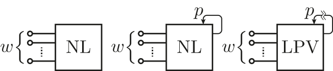
By assuming that the scheduling is (i) measurable, i.e., it can be calculated from measurable signals via , and (ii) allowed to vary independently of the other signals, such as inside a compact, convex set that defines the range of , then we can call (2) an embedding of (1). This means that the solution set of (1) is embedded in the solution set of (2). While linearity is gained by taking these assumptions on , the price to be paid is conservatism of the resulting representation, as the solution set of (2) will inevitably contain more solution trajectories than the solution set of (1), due to the assumed independence of . The LPV embedding procedure is schematically depicted in Fig. 1. With this embedding strategy, numerous successful applications of LPV control for nonlinear systems have been presented in literature (Tóth, 2010; Mohammadpour and Scherer, 2012).
In the sequel, we consider that the scheduling map and the set are known, and with the choice of , (1) can be embedded in the form of (2) with the matrix functions and and , such that and have affine dependence on :
| (3) |
where the coefficients and are real matrices with appropriate dimensions and denotes the th element of the vector . Suppose we obtain the data set from (2). Based on the results of Verhoek et al. (2022), we now show that we can construct a fully data-driven representation of (2),(3) using a that satisfies a persistence of excitation condition.
2.2 Data-driven representations
Considering (2a), (3), we can separate the coefficients from the signals as
| (4) |
With , we construct the following matrices that are associated with (4):
| (5a) | ||||
| (5b) | ||||
| where , , and , respectively. Moreover, define as | ||||
| (5c) | ||||
As (2) is linear along , we have
| (6) |
Based on this relationship, the LPV system represented by (2a), (3) can be fully characterized in terms of the data matrices in (5) as follows
| (7) |
The data-based representation (7) is well-posed under the condition that the data set is persistently exciting (PE). The PE condition for , given the representation (2),(3), is defined in Verhoek et al. (2022) as follows:
Condition \thethm
Remark 1
To satisfy Condition 2.2, we have that and, as , are known it is possible to explicitly verify the condition.
2.2.1 Closed-loop data-driven representations:
Connecting the LPV system with the feedback law , where has affine dependence on , i.e.,
| (8) |
yields the closed-loop system,
| (9) |
where , with , similarly for . With (9), we can now introduce the following result that provides data-based parametrization of the closed-loop.
Theorem 2
2.3 Data-driven controller synthesis
With the data-driven representation of the closed-loop LPV system in Theorem. 2, LPV state-feedback controller synthesis algorithms can be formulated, which generate controllers using only the information in , while guaranteeing stability and performance of the closed-loop. We consider two controller synthesis algorithms, developed in Verhoek et al. (2022), that yield guarantees in terms of quadratic stability and performance, e.g., -gain.
Before we can discuss the synthesis methods, we need to introduce a few variables that are necessary to formulate the results. For a define
| (12a) | |||
| and for in (5) define | |||
| (12b) | |||
| Furthermore, for a satisfying (11), define the matrices , as | |||
| (12c) | |||
With these variables, we can formulate the synthesis method that provides an LPV state-feedback controller that guarantees stability and quadratic performance of the closed-loop system defined by , in terms of the following theorem.
Theorem 3
Given a from (2) that satisfies Condition 2.2. There exists an LPV state-feedback controller in the form of (8) that stabilizes (2) and for a given minimizes the supremum of
along all solutions of (9), if there exist , , as in (12c), and , such that
| (13h) | |||
| (13m) | |||
| (13n) | |||
for all , where
| (14a) | ||||
| (14b) | ||||
| (14c) | ||||
| (14d) | ||||
| (14e) | ||||
| (14f) | ||||
| (14g) | ||||
| with , | ||||
and as in (12). Then, the state-feedback controller is constructed as
| (15) |
where is minimizing among all possible choices of that satisfy (13).
See Verhoek et al. (2022). Similarly, we can formulate a data-driven synthesis method that yields an LPV state-feedback controller that guarantees a bound on the -gain, shaped by matrices (see Verhoek et al. (2022)), of the closed-loop system.
Theorem 4
Given and a generated by (2) that satisfies Condition 2.2. There exists an LPV state-feedback controller in the form of (8) that stabilizes (2) and guarantees that the -gain of the closed-loop system is less than , if there exists a , a multiplier , as in (12c), and that satisfy the conditions in (13) with
| (16a) | ||||
| (16b) | ||||
| (16c) | ||||
| (16d) | ||||
| (16e) | ||||
and with as in (14), and as in (12). Then, a realization of is obtained as in (15).
2.4 Discussion
We want to again highlight that both these synthesis programs are only dependent on (i) the data set that is measured from the system, and (ii) the assumed knowledge of the scheduling map . Furthermore, when the input is sufficiently exciting, one needs only data points to be able to synthesize an LPV state-feedback controller for a nonlinear system. It is also important to note that –contrary to well-established results in model-based LPV state-feedback synthesis (Rugh and Shamma, 2000; Rotondo et al., 2014)– our synthesis methods allow to have a scheduling dependent matrix in the LPV representation (2) of the true underlying system, although such a representation/model is never computed in our methodology. Finally, the data that is used in the synthesis methods of Theorems 3 and 4 is assumed to be noise-free, just as in the initial results for LTI systems (Markovsky and Rapisarda, 2008). Extending our results to handle noise-infected data is an important future research direction. The role of regularization, as discussed in the recent paper Breschi et al. (2022), is expected to be a promising approach to further generalize this method for noisy data.
3 Experimental setup
We will now apply the discussed data-driven LPV state-feedback synthesis methods to design a controller for an experimental nonlinear unbalanced disc setup and implement the designed controller on it.
3.1 Setup description
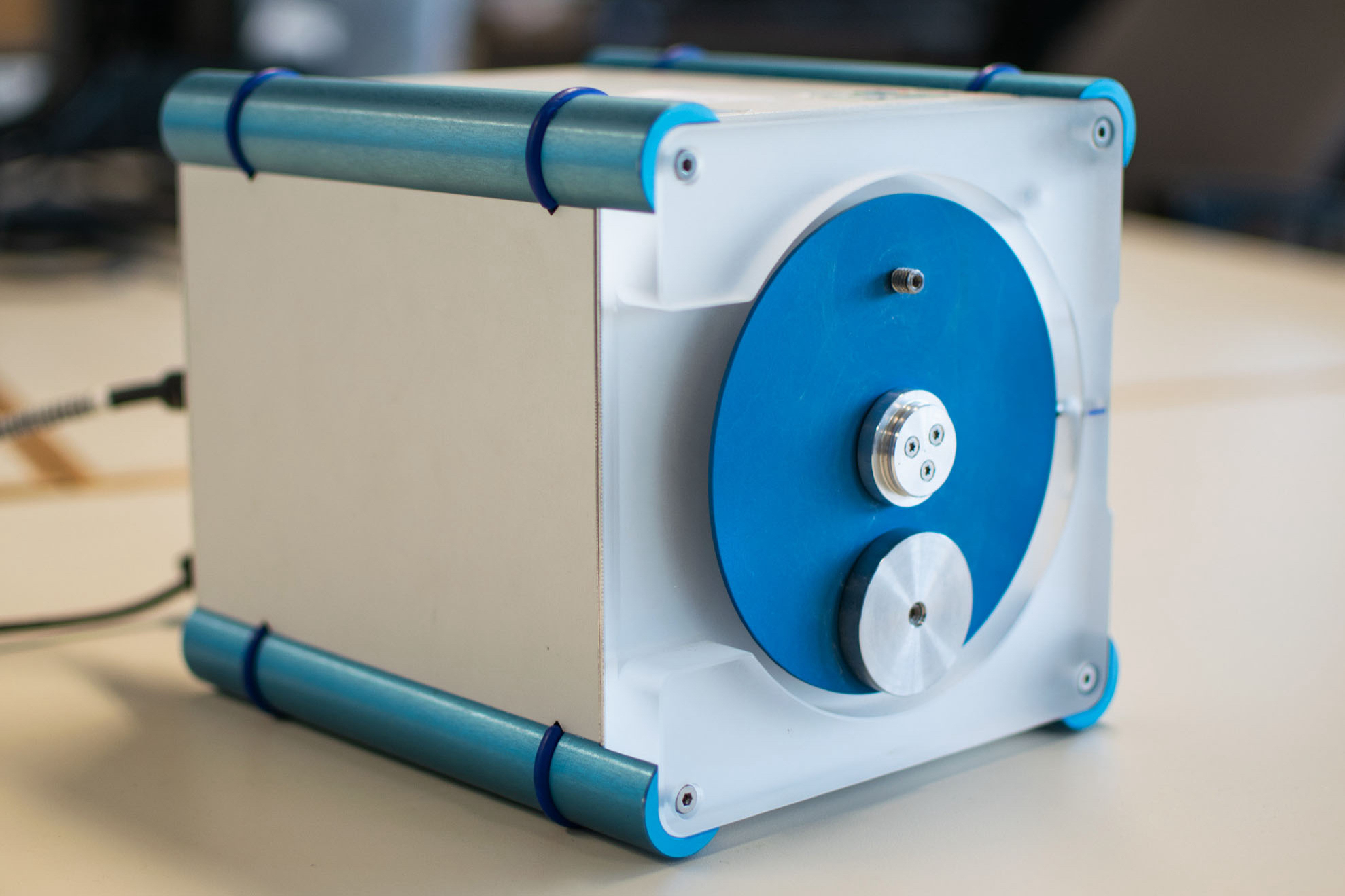
The experimental setup that we consider is an unbalanced disc system, depicted in Fig. 2. The unbalanced disc setup consists of a DC motor connected to a disc with an off-centered mass, and hence it mimics the behavior of a rotational pendulum. The angular position of the disc is measured using an incremental encoder. The continuous-time nonlinear dynamics of the unbalanced disc system are represented by the following ordinary differential equation,
| (17) |
where is the angular position of the disc, is the input voltage to the system, which is its control input, and are the physical parameters of the system. In this setup, is applied with a zero-order-hold actuation and is saturated at [V].
In Kulcsár et al. (2009); Koelewijn and Tóth (2019), the physical parameters for this setup are estimated using LPV identification methods, and model-based LPV controllers have been successfully applied to it using the estimated parameters (Abbas et al., 2021). We actuate and measure the system with synchronized sampling at a sampling time of seconds. Embedding (17) into an LPV representation can be established by defining the scheduling as , where is the scheduling map. Hence, is considered as the range of the function, i.e., . By choosing , we can write (17) as a continuous-time LPV-SS representation:
| (18a) | ||||
| (18b) | ||||
It is clear that (18) is affinely dependent on . Moreover, can be obtained through the aforementioned scheduling map by measuring with the encoder. Therefore, we can use our data-driven synthesis methods, discussed in Section 2, for the design of a DT controller for this system without knowing at all the DT equivalent of (17) under the considered , the parameter values, or (18). We only assume that , i.e., the calculated sequence of , is available.
3.2 Data generation
The system is controlled using a real-time Matlab environment on a MacBook Pro (2020), which communicates with the setup through an USB port. More details on the Matlab environment can be found in Kulcsár et al. (2009). The Matlab environment ensures synchronous actuation and measurement of the setup. We obtain the output of the incremental encoder () and an estimate of the angular speed as measurements.
We obtain our data-dictionary by exciting the system with a randomly generated input in the range , filtered through a low-pass filter to restrict the frequency range of the excitation to the normal operation range of the setup. Condition 2.2 provides that , i.e., [ms]. To account for noise induced by the encoder and the estimation error of , we gathered 1 second worth of data from which we selected our data-dictionary that is used in the synthesis algorithms.
3.3 Controller synthesis
For this experimental demonstration, we considered the design of two controllers:
From the obtained measurement data, we randomly select a window of samples, which satisfies Condition 2.2 to create our data-dictionary . Our data-dictionary is depicted in Fig. 3. As satisfies Condition 2.2, we will use it to represent the behavior of the nonlinear unbalanced disc system.
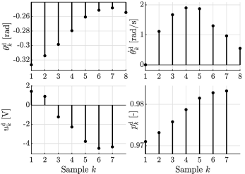
Note that the scheduling signal is calculated by propagating the measurement of through the scheduling map. From the data-dictionary, we construct the matrices according to (5), and the data-driven representation , which are used in the synthesis procedures of Theorems 3 and 4.
We are now ready to synthesize Controller 1 and Controller 2. In order to improve numerical conditioning, we re-scale and re-center the scheduling in the synthesis problems such that . Solving the synthesis problem for Controller 1 with , in Matlab, using YALMIP with solver MOSEK, yields
For numerical conditioning, we add a regularization in the cost function for the synthesis of Controller 2 in terms of . Synthesizing Controller 2 with , and yields with
Just like in model-based design, we have chosen the values for and by iterative tuning. We want to emphasize that we have been able to synthesize these LPV state-feedback controllers using only the 7 data points shown in Fig. 3. We will now implement these controllers on the experimental setup.
3.4 Experiments
For the experimental verification of our synthesized controllers, we consider two scenarios; a disturbance rejection scenario and a reference tracking scenario.
3.4.1 Disturbance rejection:
In this scenario, the controller will regulate the states of the unbalanced disc at the origin, while we disturb the system by displacing the disc by hand. We define the origin of the unbalanced disc system as the upright position. For this scenario, we only present results with Controller 1, as it was not possible to apply exactly the same disturbance for both experiments. We ran the controller online for 20 seconds, and manually disturbed the system 5 times by pulling the mass away from the upright position.
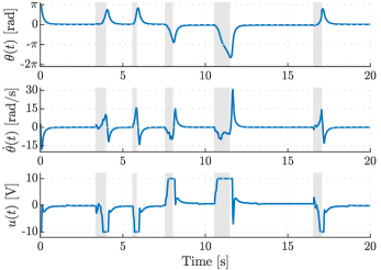
Fig. 4 shows the obtained measurement results during the experiments. The gray-shaded areas in the plots indicate the instances where we have manually disturbed the system. A video of the experiment is available at https://youtu.be/m9l61lR1Fw4. From the figure, we can conclude that the designed LPV state-feedback controller, which is synthesized using only 7 time measurements, can robustly regulate the nonlinear system at the setpoint of 0 [rad] for the full operating range.
3.4.2 Reference tracking:
In this scenario, we asses if the designed controllers can realize arbitrary setpoints for the nonlinear system. We select the sequence of setpoints as that should track in the experiment. In order to ensure reference tracking, we deploy the controllers in terms of
| (19) |
Note that we do not apply a feedforward term here, i.e., the controller considers to be equilibrium points. Running the experiment for 20 seconds with either Controller 1 or Controller 2 interconnected with the setup yields the measurements plotted in Fig. 5. A video of the experiments is available at https://youtu.be/SyyUVy1sPsc.
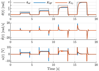
The results show that the closed-loop system achieves reference tracking along the full operating range of the nonlinear system with an LPV controller that is designed using only 7 data-points recorded from the system. Note however that due to the lack of integral action or a feedforward term, there is a small steady-state error for some reference points, which is in accordance with the theory of standard state-feedback design.
3.5 Discussion
We have shown that the designed LPV controllers can achieve the stability and performance objectives on the nonlinear system. This is accomplished by measuring a data-dictionary of input-scheduling-state data, where the scheduling is constructed using a given scheduling map. Although, the current results assume the data is noise free, as was the case in the initial results on LTI system, our experimental results show that there is a certain level of robustness of the data-driven control laws that are obtained via this design procedure. However, proper guarantees of performance and stability of the closed-loop are not available in case of noise-infected data. We want to note that the synthesis algorithms gave numerical problems for some of the selected windows from the original 1-second-long data set. Hence, even though persistency of excitation holds in terms of a rank condition, it does matter that what the conditioning number is associated with ‘’, i.e., the amount of relative information present in the chosen window. A more quantitative measure of information content in the data could certainly be useful to avoid such numerical difficulties.
4 Conclusions and outlook
The experimental results presented in this work demonstrate that direct data-driven control of nonlinear systems can be established via LPV data-driven methods. Furthermore, for the deployed LPV data-driven control design for the unbalanced disc system, only 7 data-points are required to ensure stability and performance on the setup. A next step for further improvement of the proposed methodology is to make it robust to noisy data.
References
- Abbas et al. (2021) Abbas, H.S., Tóth, R., Petreczky, M., Meskin, N., Mohammadpour Velni, J., and Koelewijn, P.J.W. (2021). LPV modeling of nonlinear systems: A multi-path feedback linearization approach. International Journal of Robust and Nonlinear Control, 31(18), 9436–9465.
- Alsalti et al. (2021) Alsalti, M., Berberich, J., Lopez, V.G., Allgöwer, F., and Müller, M.A. (2021). Data-Based System Analysis and Control of Flat Nonlinear Systems. In Proc. of the 60th IEEE Conference on Decision and Control, 1484–1489.
- Breschi et al. (2022) Breschi, V., Chiuso, A., and Formentin, S. (2022). The role of regularization in data-driven predictive control. arXiv preprint arXiv:2203.10846.
- Coulson et al. (2019) Coulson, J., Lygeros, J., and Dörfler, F. (2019). Data-enabled predictive control: In the shallows of the DeePC. In Proc. of the European Control Conference, 307–312.
- De Persis and Tesi (2019) De Persis, C. and Tesi, P. (2019). Formulas for Data-Driven Control: Stabilization, Optimality, and Robustness. IEEE Trans. on Automatic Control, 65(3), 909–924.
- Koelewijn and Tóth (2019) Koelewijn, P.J.W. and Tóth, R. (2019). Physical parameter estimation of an unbalanced disc system. Technical Report TUE CS, Eindhoven University of Technology.
- Kulcsár et al. (2009) Kulcsár, B., Dong, J., van Wingerden, J.W., and Verhaegen, M. (2009). LPV subspace identification of a DC motor with unbalanced disc. In Proc. of the 15th IFAC Symposium on System Identification, 856–861.
- Markovsky and Dörfler (2021) Markovsky, I. and Dörfler, F. (2021). Behavioral systems theory in data-driven analysis, signal processing, and control. Annual Reviews in Control, 52, 42–64.
- Markovsky and Rapisarda (2008) Markovsky, I. and Rapisarda, P. (2008). Data-Driven Simulation and Control. International Journal of Control, 81(12), 1946–1959.
- Mohammadpour and Scherer (2012) Mohammadpour, J. and Scherer, C.W. (eds.) (2012). Control of Linear Parameter Varying Systems with Applications. Springer.
- Romer et al. (2019) Romer, A., Berberich, J., Köhler, J., and Allgöwer, F. (2019). One-Shot Verification of Dissipativity Properties from Input–Output Data. IEEE Control Systems Letters, 3(3), 709–714.
- Rotondo et al. (2014) Rotondo, D., Nejjari, F., and Puig, V. (2014). Robust state-feedback control of uncertain LPV systems: An LMI-based approach. Journal of the Franklin Institute, 351(5), 2781–2803.
- Rugh and Shamma (2000) Rugh, W.J. and Shamma, J.S. (2000). Research on gain scheduling. Automatica, 36(10), 1401–1425.
- Tóth (2010) Tóth, R. (2010). Modeling and Identification of Linear Parameter-Varying Systems. Springer.
- Verhoek et al. (2021a) Verhoek, C., Abbas, H.S., Tóth, R., and Haesaert, S. (2021a). Data-Driven Predictive Control for Linear Parameter-Varying Systems. In Proc. of the 4th IFAC Workshop on Linear Parameter Varying Systems, volume 54.
- Verhoek et al. (2023) Verhoek, C., Berberich, J., Haesaert, S., Allgöwer, F., and Tóth, R. (2023). Data-driven Dissipativity Analysis of Linear Parameter-Varying Systems. arXiv preprint: arXiv:2303.10031.
- Verhoek et al. (2022) Verhoek, C., Tóth, R., and Abbas, H.S. (2022). Direct Data-Driven State-Feedback Control of Linear Parameter-Varying Systems. arXiv preprint: arXiv:2211.17182.
- Verhoek et al. (2021b) Verhoek, C., Tóth, R., Haesaert, S., and Koch, A. (2021b). Fundamental Lemma for Data-Driven Analysis of Linear Parameter-Varying Systems. In Proc. of the 60th IEEE Conference on Decision and Control, 5040–5046.
- Willems et al. (2005) Willems, J.C., Rapisarda, P., Markovsky, I., and De Moor, B.L.M. (2005). A note on persistency of excitation. Systems & Control Letters, 54(4), 325–329.