Direct Data-Driven State-Feedback Control of Linear Parameter-Varying Systems

Abstract

We derive novel methods that allow to synthesize LPV state-feedback controllers directly from a single sequence of data and guarantee stability and performance of the closed-loop system, without knowing the model of the plant. We show that if the measured open-loop data from the system satisfies a persistency of excitation condition, then the full open-loop and closed-loop input-scheduling-state behavior can be represented using only the data. With this representation, we formulate synthesis problems that yield controllers that guarantee stability and performance in terms of infinite horizon quadratic cost, generalized $\mathcal{H}_{2}$-norm and $\ell_{2}$-gain of the closed-loop system. The controllers are synthesized by solving an SDP with a finite set of LMI constraints. Competitive performance of the proposed data-driven synthesis methods is demonstrated w.r.t. model-based synthesis that have complete knowledge of the true system model in multiple simulation studies.

Data-Driven Control, Linear Parameter-Varying Systems, Behavioral systems, $\mathcal{H}_{\infty}$ control, State-Feedback Control.

1 Introduction

Due to increasing performance, environmental, etc., requirements, control of new generations of engineering systems is increasingly more challenging, as the dynamic behaviors of these systems is becoming dominated by nonlinear (NL) effects. A particularly interesting framework to deal with such challenges is the class of linear parameter-varying (LPV) systems [1]. LPV systems have a linear input-(state)-output relationship, but this relationship itself is dependent on a measurable, time-varying signal, referred to as the scheduling signal. This scheduling signal is used to express the NL/time-varying/exogenous components that are affecting the system, allowing to describe a wide range of NL systems in terms of LPV surrogate models [1]. In practice, LPV modeling and model-based control methods have been successfully deployed in many engineering problems, proving versatility of the framework to meet with the increasing complexity challenges and performance expectations [2].

However, despite of the powerful LPV model-based control solutions, their deployment is becoming more challenging, as modeling of the next generation of engineering systems via first-principles is increasingly complex, time-consuming and often lacks sufficient accuracy. Hence, engineers frequently need to obtain models based on data to analyze and control such systems. Despite the tremendous progress in LPV and NL model identification, e.g., [1, 3, 4, 5, 6, 7, 8, 9], several aspects of the model identification toolchain such as model structure selection, are either under-developed or are rather complex and demand several iterations. Moreover, research on identification for control in the linear time-invariant (LTI) case has shown that, to synthesize a controller to achieve a given performance objective in model-based control, only some dynamical aspects of the system are important [10]. This means that focusing the identification process on obtaining only such information accurately for synthesis can achieve higher model-based control performance for a given experimentation budget. This lead to the idea that fusing the control objective into system identification and even accomplishing synthesis of a controller directly from data, i.e., direct data-driven control, carries many benefits [11], while it also simplifies the overall modeling and control toolchain. Based on this motivation, data-driven LPV control methods [12, 13, 14] have been introduced, which have provided promising solutions to the direct control design problem, however, often without guarantees on the stability and performance of the resulting closed-loop system.

In the LTI case, a cornerstone result, the so-called Fundamental Lemma [15], allows the design of direct data-driven controllers with closed-loop stability and performance guarantees. Using this lemma, numerous powerful results have been developed for LTI systems on data-driven simulation [16], stability and performance analysis [17, 18, 19], and (predictive) control [20, 21, 22], many of which also provide robustness against noise. The extension of Willems’ Fundamental Lemma for the class of LPV systems has been derived in [23, 24] and it has already been used for the development of direct LPV data-driven predictive control design [24] and direct data-driven dissipativity analysis of LPV systems [25]. In this work, we further extend this promising approach with the development of data-driven LPV state-feedback controller synthesis methods that can provide closed-loop stability and performance guarantees based on just a single sequence of measurement data from the system. More specifically, our contributions in this paper are:

1. Deriving data-driven open- and closed-loop LPV representations from a single sequence of input-scheduling-state measurement data of an unknown LPV system that has a state-space representation with affine dependence;

2. Development of fully data-based analysis and synthesis methods of LPV state-feedback controllers to guarantee closed-loop stability;

3. Development of direct data-driven analysis and synthesis methods of LPV state-feedback controllers with guaranteed quadratic, $\mathcal{H}^{\mathrm{g}}_{2}$-norm and $\ell_{2}$-gain-based performance of the closed-loop.

The data-driven analysis and synthesis techniques that we present in this paper can be efficiently solved as a semi-definite program (SDP), subject to a finite set of linear matrix inequalities (LMIs), which are constructed using only the measurement data from the unknown LPV system.

The paper is structured as follows: the problem setting is introduced in Section 2, followed by the open- and closed-loop data-driven LPV representations in Section 3, providing C1. Based on the derived representations, the direct LPV data-driven controller synthesis methods are formulated in Section 4 and 5, giving C2 and C3. We finish the paper with a comparative simulation study in Section 6, demonstrating competitive performance of the proposed methods. Finally, the conclusions are drawn in Section 7.

Notation

The identity matrix is denoted by $I_{n}\in\mathbb{R}^{n\times n}$, while $1_{n}$ denotes the vector $\begin{bmatrix}1&\cdots&1\end{bmatrix}^{\top}\in\mathbb{R}^{n}$. $X\succ 0$ and $X\prec 0$ ($X\succeq 0$ and $X\preceq 0$) denote positive/negative (semi) definiteness of a symmetric matrix $X\in\mathbb{R}^{n\times n}$, respectively. The Kronecker product of $A\in\mathbb{R}^{n\times m}$ and $B\in\mathbb{R}^{p\times q}$ is denoted by $A\otimes B\in\mathbb{R}^{pm\times qn}$, and for $C\in\mathbb{R}^{m\times k}$, $D\in\mathbb{R}^{q\times l}$, the following identity holds [26]:

$$(A\otimes B)(C\otimes D)=AC\otimes BD.$$ (1)

The Redheffer star product is $\Delta\star L$, which for $\Delta\in\mathbb{R}^{n\times m}$ and $L\in\mathbb{R}^{p\times q}$ with $n<p$ and $m<q$ gives the upper linear fractional transformation (LFT). Furthermore, the Moore-Penrose (right) pseudo-inverse is denoted by $\dagger$. We use $(*)$ to denote a symmetric term in a quadratic expression, e.g. $(*)^{\top}Q(a-b)=(a-b)^{\top}Q(a-b)$ for $Q\in\mathbb{R}^{n\times n}$ and $a,b\in\mathbb{R}^{n}$. Block diagonal concatenation of matrices is given by $\mathrm{blkdiag}$.

2 Problem setting

Consider a discrete-time LPV system that can be represented by the following LPV-SS representation:

$$x_{k+1} =A(p_{k})x_{k}+B(p_{k})u_{k},$$ (2a)

$$y_{k} =x_{k},$$ (2b)

where $k\in\mathbb{Z}$ is the discrete time, $x_{k}\in\mathbb{R}^{n_{\mathrm{x}}}$, $u_{k}\in\mathbb{R}^{n_{\mathrm{u}}}$, $y_{k}\in\mathbb{R}^{n_{\mathrm{x}}}$ and $p_{k}\in\mathbb{P}$ are the state, input, output and scheduling signals, respectively, and $\mathbb{P}\subset\mathbb{R}^{n_{\mathrm{p}}}$ is a compact, convex set which defines the range of the scheduling signal. The matrix functions $A:\mathbb{P}\rightarrow\mathbb{R}^{n_{\mathrm{x}}\times n_{\mathrm{x}}}$ and $B:\mathbb{P}\rightarrow\mathbb{R}^{n_{\mathrm{x}}\times n_{\mathrm{u}}}$ are considered to have affine dependency on $p_{k}$, which is a common assumption in practice, cf. [27, 28],

$$A(p_{k})=A_{0}+\sum_{i=1}^{n_{\mathrm{p}}}p_{k,i}A_{i},\quad B(p_{k})=B_{0}+\sum_{i=1}^{n_{\mathrm{p}}}p_{k,i}B_{i},$$ (3)

where $\{A_{i}\}_{i=1}^{n_{\mathrm{p}}}$ and $\{B_{i}\}_{i=1}^{n_{\mathrm{p}}}$ are real matrices with appropriate dimensions. In terms of solutions of (2), we consider

$$\mathfrak{B}=\{(x,p,u)\in(\mathbb{R}^{n_{\mathrm{x}}}\times\mathbb{P}\times\mathbb{R}^{n_{\mathrm{u}}})^{\mathbb{Z}}\mid\text{\eqref{eq:LPVSS} holds }\forall k\in\mathbb{Z}\}.$$ (4)

To stabilize (2), we can design an LPV state-feedback controller $K(p_{k})$ corresponding to the control-law

$$u_{k}=K(p_{k})x_{k},$$ (5a)

where we choose the LPV state-feedback controller $$K:\mathbb{P}\to\mathbb{R}^{n_{\mathrm{u}}\times n_{\mathrm{x}}} p_{k}$$ to have affine dependence on

$$K(p_{k})=K_{0}+{\textstyle\sum_{i=1}^{n_{\mathrm{p}}}}p_{k}^{[i]}K_{i},$$ (5b)

similar to (2). The well-known state-feedback problem is to design $K(p_{k})$ such that it ensures asymptotic (input-to-state) stability and minimizes a given performance measure (e.g., $\ell_{2}$-gain) of the closed-loop system

$$x_{k+1}=A_{\textsc{CL}}(p_{k})x_{k}=\left(A(p_{k})+B(p_{k})K(p_{k})\right)x_{k},$$ (6)

under all scheduling trajectories $p\in\mathbb{P}^{\mathbb{Z}}$, where the solution set of (6) is $\mathfrak{B}_{\mathrm{CL}}=\mathfrak{B}|_{u=K(p)x}\subseteq\mathfrak{B}_{x,p}$. For such a design of $K(p_{k})$, one will need the exact mathematical description of (2), which can be unrealistic in practical situations. In this paper, we consider the design of $K(p_{k})$ for an unknown LPV system (2), based only on the measured data-set

$$\mathcal{D}_{N_{\mathrm{d}}}\coloneq\{u_{k}^{\mathrm{d}},p_{k}^{\mathrm{d}},x_{k}^{\mathrm{d}}\}_{k=1}^{N_{\mathrm{d}}},$$ (7)

which is a single trajectory from (2). This problem is formalized in the following problem statement.

Problem statement

Consider a data-generating system that can be represented with (2). Given the data-dictionary $\mathcal{D}_{N_{\mathrm{d}}}$ sampled from the data-generating system. How to synthesize a state-feedback controller $K(p_{k})$, based on only $\mathcal{D}_{N_{\mathrm{d}}}$, that ensures stability and performance of the closed-loop (6)?

In order to solve this problem, we first need to construct data-driven representations of $\mathfrak{B}$ and $\mathfrak{B}_{\mathrm{CL}}$, i.e., data-based realizations of (2) and (6), corresponding to Contribution C1.

3 Data-Driven LPV Representations

In this section, we derive novel data-driven LPV-SS representations that we will use for state-feedback controller design. These results can be seen as the state-space counterpart of data-driven LPV-IO representations used in [23, 24]. Based only on the data-dictionary $\mathcal{D}_{N_{\mathrm{d}}}$, we construct data-driven representations of both the open-loop (2) and the closed-loop (6) systems, allowing later to derive controller synthesis algorithms using only the information in $\mathcal{D}_{N_{\mathrm{d}}}$.

3.1 Open-loop data-driven LPV representation

First note that by separating the coefficient matrices in (3) from the signals in (2), we can rewrite the state equation (2a) by introducing auxiliary signals $p_{k}\otimes x_{k}$ and $p_{k}\otimes u_{k}$:

$$x_{k+1}=\mathcal{A}\begin{bmatrix}x_{k}\\ p_{k}\otimes x_{k}\end{bmatrix}+\mathcal{B}\begin{bmatrix}u_{k}\\ p_{k}\otimes u_{k}\end{bmatrix},$$ (8)

where $\mathcal{A}=\begin{bmatrix}A_{0}&A_{1}&\cdots&A_{n_{\mathrm{p}}}\end{bmatrix}$, $\mathcal{B}=\begin{bmatrix}B_{0}&B_{1}&\cdots&B_{n_{\mathrm{p}}}\end{bmatrix}$. Then, given the measured data-dictionary $\mathcal{D}_{N_{\mathrm{d}}}$ from (2), the construction of the following matrices

$$U=\begin{bmatrix}u^{\mathrm{d}}_{1}&\cdots&u^{\mathrm{d}}_{{N_{\mathrm{d}}}-1}\end{bmatrix},\quad X=\begin{bmatrix}x^{\mathrm{d}}_{1}&\cdots&x^{\mathrm{d}}_{{N_{\mathrm{d}}}-1}\end{bmatrix},$$ (9a)

$$U^{\mathtt{p}}=\begin{bmatrix}p^{\mathrm{d}}_{1}\otimes u^{\mathrm{d}}_{1}&\cdots&p^{\mathrm{d}}_{{N_{\mathrm{d}}}-1}\otimes u^{\mathrm{d}}_{{N_{\mathrm{d}}}-1}\end{bmatrix},$$ (9b)

$$X^{\mathtt{p}}=\begin{bmatrix}p^{\mathrm{d}}_{1}\otimes x^{\mathrm{d}}_{1}&\cdots&p^{\mathrm{d}}_{{N_{\mathrm{d}}}-1}\otimes x^{\mathrm{d}}_{{N_{\mathrm{d}}}-1}\end{bmatrix},$$ (9c)

$$\overrightarrow{X}=\begin{bmatrix}x^{\mathrm{d}}_{2}&\cdots&x^{\mathrm{d}}_{{N_{\mathrm{d}}}}\end{bmatrix},$$ (9d)

where $U^{\mathtt{p}}\!\in\!\mathbb{R}^{n_{\mathrm{p}}n_{\mathrm{u}}\times{N_{\mathrm{d}}}-1},U\!\in\!\mathbb{R}^{n_{\mathrm{u}}\times{N_{\mathrm{d}}}-1}$, $X^{\mathtt{p}}\!\in\!\mathbb{R}^{n_{\mathrm{p}}n_{\mathrm{x}}\times{N_{\mathrm{d}}}-1}$ and $X,\overrightarrow{X}\in\mathbb{R}^{n_{\mathrm{x}}\times{N_{\mathrm{d}}}-1}$, allows to write the relationship between the system parameters $\mathcal{A},\mathcal{B}$ and the data in $\mathcal{D}_{N_{\mathrm{d}}}$ as

$$\overrightarrow{X}=\mathcal{A}\begin{bmatrix}X\\ X^{\mathtt{p}}\end{bmatrix}+\mathcal{B}\begin{bmatrix}U\\ U^{\mathtt{p}}\end{bmatrix}.$$ (10)

Note that (10) holds true due to the linearity property of LPV systems along a given $p$ trajectory. This is a well-known fact and often used in LPV subspace identification, cf. [29]. Instead of estimating the system parameters $\mathcal{A},\mathcal{B}$ (as is done in LPV system identification), we now represent the LPV system (2) with $\mathcal{D}_{N_{\mathrm{d}}}$ using the data matrices (9):

$$x_{k+1}=\overrightarrow{X}\mathcal{G}^{\dagger}\begin{bmatrix}x_{k}\\ p_{k}\otimes x_{k}\\ u_{k}\\ p_{k}\otimes u_{k}\end{bmatrix},\quad\mathcal{G}:=\begin{bmatrix}X\\ X^{\mathtt{p}}\\ U\\ U^{\mathtt{p}}\end{bmatrix}.$$ (11)

Note that from this data-driven representation, the relation $\begin{bmatrix}\mathcal{A}&\mathcal{B}\end{bmatrix}=\overrightarrow{X}\mathcal{G}^{\dagger}$ is recovered – a well-established result in LPV subspace identification literature [29, 30]. The key observation is that in, e.g., [30], $\mathcal{A},\mathcal{B}$ are identified by minimizing $\|\overrightarrow{X}-\begin{bmatrix}\mathcal{A}&\mathcal{B}\end{bmatrix}\mathcal{G}\|$ in some norm. This estimation procedure can easily throw away important information that is encoded in the data. In contrast, we use the data in (11) directly as a representation, avoiding any loss of information.

The data-based representation (11) is well-posed under the condition that the data-set $\mathcal{D}_{N_{\mathrm{d}}}$ is persistently exciting (PE). Note that the PE condition is always defined with respect to a certain system class/representation, which is in this case a static-affine LPV-SS representation with full state observation. Contrary to the PE condition for shifted-affine LPV-IO representations [23], the PE condition for the system class considered in this paper is simpler, and corresponds to the existence of the right pseudo-inverse $\mathcal{G}^{\dagger}$ of $\mathcal{G}$, giving the following PE condition for $\mathcal{D}_{N_{\mathrm{d}}}$ to imply existence of (11):

Condition 1 (Persistency of Excitation).

If $\mathcal{G}$ has full row rank, i.e., $\mathrm{rank}\!\left(\mathcal{G}\right)=(1+n_{\mathrm{p}})(n_{\mathrm{x}}+n_{\mathrm{u}})$, then $\mathcal{D}_{N_{\mathrm{d}}}$ is persistently exciting w.r.t. (2) and (3). $\square$

Based on this condition, we need at least ${N_{\mathrm{d}}}\geq(1+n_{\mathrm{p}})(n_{\mathrm{x}}+n_{\mathrm{u}})$ data points for (11). Moreover, as we assume full state observation, the parameters $n_{\mathrm{x}},n_{\mathrm{p}},n_{\mathrm{u}}$ are also known and thus no additional conditions are required to ensure existence of (11).

3.2 Closed-loop data-driven LPV representation

Next, we derive a data-driven representation of the closed-loop system (6), where (2) with (3) is controlled via the feedback law (5), where the controller has static-affine dependence, as defined in (5b). The following theorem gives conditions such that we can represent (6) using only the data-set $\mathcal{D}_{N_{\mathrm{d}}}$, i.e., this result provides a data-based parameterization of the closed-loop system with the state-feedback law (5).

Theorem 1 (Data-based closed-loop rep.).

Given the data-dictionary $\mathcal{D}_{N_{\mathrm{d}}}=\{u_{k},p_{k},x_{k}\}_{k=1}^{{N_{\mathrm{d}}}}$, measured from (2) and satisfying Condition 1. Let $\overrightarrow{X}$ and $\mathcal{G}$ be defined as in (9d) and (11), under $\mathcal{D}_{N_{\mathrm{d}}}$. For an LPV controller $K$ given by (5), the closed-loop system (6) is represented equivalently as

$$x_{k+1}=\overrightarrow{X}\mathcal{V}\begin{bmatrix}x_{k}\\ p_{k}\otimes x_{k}\\ p_{k}\otimes p_{k}\otimes x_{k}\end{bmatrix},$$ (12)

where $\mathcal{V}\in\mathbb{R}^{{N_{\mathrm{d}}}-1\times n_{\mathrm{x}}(1+n_{\mathrm{p}}+n_{\mathrm{p}}^{2})}$ is any matrix that satisfies

$$\mathcal{M}_{\textsc{CL}}:=\begin{bmatrix}I_{n_{\mathrm{x}}}&0&0\\ 0&I_{n_{\mathrm{p}}}\otimes I_{n_{\mathrm{x}}}&0\\ K_{0}&\bar{K}&0\\ 0&I_{n_{\mathrm{p}}}\otimes K_{0}&I_{n_{\mathrm{p}}}\otimes\bar{K}\end{bmatrix}=\begin{bmatrix}X\\ X^{\mathtt{p}}\\ U\\ U^{\mathtt{p}}\end{bmatrix}\mathcal{V}.$$ (13)

Proof.

We first write the controller (5) as

$$u_{k}=\mathcal{K}\begin{bmatrix}x_{k}\\ p_{k}\otimes x_{k}\end{bmatrix},\quad\mathcal{K}=\begin{bmatrix}K_{0}&K_{1}&\cdots&K_{n_{\mathrm{p}}}\end{bmatrix},$$ (14)

such that, when substituted in (6), we obtain the closed-loop

$$x_{k+1}=\begin{bmatrix}A_{0}&\bar{A}\end{bmatrix}\begin{bmatrix}x_{k}\\ p_{k}\otimes x_{k}\end{bmatrix}+B_{0}\mathcal{K}\begin{bmatrix}x_{k}\\ p_{k}\otimes x_{k}\end{bmatrix}\\ +\bar{B}\cdot\big{(}p_{k}\otimes(K_{0}x_{k}+\bar{K}p_{k}\otimes x_{k})\big{)},$$ (15)

where $\bar{A}=\begin{bmatrix}A_{1}&\cdots&A_{n_{\mathrm{p}}}\end{bmatrix}$, similarly for $\bar{B},\bar{K}$. Using the Kronecker property 1, we can rewrite (15) as

$$x_{k+1}\!=\!\underbrace{\begin{bmatrix}A_{0}+B_{0}K_{0}&\bar{A}+B_{0}\bar{K}+\bar{B}(I_{n_{\mathrm{p}}}\otimes K_{0})&\bar{B}(I_{n_{\mathrm{p}}}\otimes\bar{K})\end{bmatrix}}_{\mathcal{M}}\begin{bmatrix}x_{k}\\ p_{k}\otimes x_{k}\\ p_{k}\otimes p_{k}\otimes x_{k}\end{bmatrix},$$

where $\mathcal{M}$ now fully defines the relationship between the signals in the closed-loop LPV system. $\mathcal{M}$ can be rewritten as

$$\mathcal{M}=\begin{bmatrix}\mathcal{A}&\mathcal{B}\end{bmatrix}\mathcal{M}_{\textsc{CL}}.$$ (16)

Substituting the relation $\begin{bmatrix}\mathcal{A}&\mathcal{B}\end{bmatrix}=\overrightarrow{X}\mathcal{G}^{\dagger}$ and (13) into (16) yields $\mathcal{M}=\overrightarrow{X}\mathcal{V}$, which, through (15), gives the data-based closed-loop representation (12), equivalent to the model-based closed-loop representation (6). ∎

Note that, under Condition 1, $\mathcal{V}=\mathcal{G}^{\dagger}\mathcal{M}_{\textsc{CL}}$ would be only a particular (minimum 2-norm solution) of (13), while Theorem 1 allows for an affine subspace of solutions in terms of $\mathcal{V}$ in the orthogonal projection of $\mathcal{M}_{\textsc{CL}}$ on the range of $\mathcal{G}$. Furthermore, for a given $\mathcal{V}$, condition (13) allows to recover the controller $K(p_{k})$. To this end, let us introduce a partitioning of $\mathcal{V}:=\begin{bmatrix}V_{0}&\bar{V}&\bar{\bar{V}}\end{bmatrix}$, with

$$\bar{V}=\begin{bmatrix}V_{1}&\cdots&V_{n_{\mathrm{p}}}\end{bmatrix},\quad\bar{\bar{V}}=\begin{bmatrix}V_{n_{\mathrm{p}}+1}&\cdots&V_{n_{\mathrm{pp}}}\end{bmatrix},$$

such that, via (13), we have

$$K_{0}=UV_{0},\quad\bar{K}=U\bar{V}.$$

Hence, the control law can be recovered, and is fully defined in terms of the data $\mathcal{D}_{N_{\mathrm{d}}}$ as

$$u_{k}=U\begin{bmatrix}V_{0}&\bar{V}\end{bmatrix}\begin{bmatrix}x_{k}\\ p_{k}\otimes x_{k}\end{bmatrix}.$$

Note that, in order to represent the control law, the term $\bar{\bar{V}}$ is redundant and only required to fulfill the data relations in (13). We will now derive synthesis algorithms that allows us to find $\mathcal{V}$, and thus synthesize LPV state-feedback controllers using only the information in $\mathcal{D}_{N_{\mathrm{d}}}$.

4 Data-driven synthesis of stabilizing LPV controllers

Based on the data-driven representation of the closed-loop system, developed in Section 3.2, we will derive data-driven controller synthesis methods that can be solved as an SDP. We show that the controllers synthesized by these methods ensure closed-loop stability and can achieve a wide range of performance targets. We first solve the direct data-driven stability analysis problem, from which the synthesis methods for stabilizing LPV state-feedback control can be derived via an extension of Lemma .2.1. This is followed by the derivation of the direct data-driven methods that allow to design LPV state-feedback controllers with different performance targets.

4.1 Closed-loop data-driven stability analysis

We first solve the direct data-driven stability analysis problem. Consider a state-feedback controller $K(p_{k})$ as in (5). Based on the model-based stability analysis condition, e.g., [31], we can use (16) to characterize closed-loop stability via

$$\begin{bmatrix}Z&ZM^{\top}(p)\\ M(p)Z&Z\end{bmatrix}\succ 0,\quad M(p)=\mathcal{M}\begin{bmatrix}I_{n_{\mathrm{x}}}\\ p\otimes I_{n_{\mathrm{x}}}\\ p\otimes p\otimes I_{n_{\mathrm{x}}}\end{bmatrix},$$ (17)

for all $p\in\mathbb{P}$ with $0\prec Z\in\mathbb{R}^{n_{\mathrm{x}}\times n_{\mathrm{x}}}$. This allows us to use the closed-loop representation in Theorem 1 to derive the following theorem, which provides a computable method to analyze the stability of the unknown LPV system in closed-loop with $K(p_{k})$ in a fully data-driven setting.

Theorem 2 (Data-driven feedback stability analysis).

Given a data-set $\mathcal{D}_{N_{\mathrm{d}}}$, satisfying Condition 1, from a system that can be represented by (2). For a $Z=Z^{\top}\in\mathbb{R}^{n_{\mathrm{x}}\times n_{\mathrm{x}}}$, let $\mathcal{F}\in\mathbb{R}^{{N_{\mathrm{d}}}-1\times n_{\mathrm{x}}(1+n_{\mathrm{p}}+n_{\mathrm{p}}^{2})}$ and $F_{Q}\in\mathbb{R}^{({N_{\mathrm{d}}}-1)(1+n_{\mathrm{p}})\times n_{\mathrm{x}}(1+n_{\mathrm{p}})}$ be defined such that

$$\mathcal{V}\begin{bmatrix}I_{n_{\mathrm{x}}}\\ p\otimes I_{n_{\mathrm{x}}}\\ p\otimes p\otimes I_{n_{\mathrm{x}}}\end{bmatrix}Z=\mathcal{F}\begin{bmatrix}I_{n_{\mathrm{x}}}\\ p\otimes I_{n_{\mathrm{x}}}\\ p\otimes p\otimes I_{n_{\mathrm{x}}}\end{bmatrix}=\begin{bmatrix}I_{{N_{\mathrm{d}}}-1}\\ p\otimes I_{{N_{\mathrm{d}}}-1}\end{bmatrix}^{\!\top}\!\!F_{Q}\begin{bmatrix}I_{n_{\mathrm{x}}}\\ p\otimes I_{n_{\mathrm{x}}}\end{bmatrix}.$$ (18)

Then the LPV state-feedback controller $K(p)$ stabilizes (2) under the feedback-law (5), if there exists an $F_{Q}$, a $Z\succ 0$ and a multiplier $\Xi=\Xi^{\top}$ which satisfy

$$\mathcal{M}_{\textsc{CL}}\begin{bmatrix}{Z}&0&0\\ 0&I_{n_{\mathrm{p}}}\otimes{Z}&0\\ 0&0&I_{n_{\mathrm{p}}}\otimes I_{n_{\mathrm{p}}}\otimes{Z}\end{bmatrix}=\mathcal{G}\mathcal{F},$$ (19)

and the LMI conditions in (47), with $\Delta(p)=\mathrm{diag}(p)\otimes I_{2n_{\mathrm{x}}}$, and where $W$ and $L_{11},\dots,L_{22}$ are given by:

$$W =\begin{bmatrix}Z_{0}&F_{Q}^{\top}{\overrightarrow{\mathcal{X}}}^{\top}\\ {\overrightarrow{\mathcal{X}}}F_{Q}&Z_{0}\end{bmatrix},\ \begin{array}[]{l}Z_{0}=\mathrm{diag}(Z,0),\vphantom{\Big{)}}\\ {\overrightarrow{\mathcal{X}}}\hskip 1.31166pt=\mathrm{diag}(\overrightarrow{X},I_{n_{\mathrm{p}}}\otimes\overrightarrow{X}),\end{array}$$ (22)

$$L_{11} =0_{2n_{\mathrm{x}}n_{\mathrm{p}}\times 2n_{\mathrm{x}}n_{\mathrm{p}}},\hskip 26.26756ptL_{12}=1_{n_{\mathrm{p}}}\otimes I_{2n_{\mathrm{x}}},$$

$$L_{21} =\begin{bmatrix}0_{n_{\mathrm{x}}\times 2n_{\mathrm{x}}n_{\mathrm{p}}}\\ I_{n_{\mathrm{p}}}\otimes\Gamma_{1}\\ 0_{n_{\mathrm{x}}\times 2n_{\mathrm{x}}n_{\mathrm{p}}}\\ I_{n_{\mathrm{p}}}\otimes\Gamma_{2}\end{bmatrix},\hskip 24.4466ptL_{22}=\begin{bmatrix}\Gamma_{1}\\ 1_{n_{\mathrm{p}}}\otimes 0_{n_{\mathrm{x}}\times 2n_{\mathrm{x}}}\\ \Gamma_{2}\\ 1_{n_{\mathrm{p}}}\otimes 0_{n_{\mathrm{x}}\times 2n_{\mathrm{x}}}\end{bmatrix},$$

$$\Gamma_{1} =\begin{bmatrix}I_{n_{\mathrm{x}}}&0\end{bmatrix},\hskip 48.04245pt\Gamma_{2}=\begin{bmatrix}0&I_{n_{\mathrm{x}}}\end{bmatrix}.$$ (23)

Proof.

Substituting the relation (16) of the data-based closed-loop representation into (17) results in

$$\begin{bmatrix}Z&ZV^{\top}\!(p)\overrightarrow{X}^{\top}\\ \overrightarrow{X}V(p)Z&Z\end{bmatrix}\succ 0,\quad\forall p\in\mathbb{P},$$ (24)

where

$$V(p)=\mathcal{V}\begin{bmatrix}I_{n_{\mathrm{x}}}\\ p\otimes I_{n_{\mathrm{x}}}\\ p\otimes p\otimes I_{n_{\mathrm{x}}}\end{bmatrix}$$

and $\mathcal{V}$ is restricted by (13), corresponding to $\mathcal{M}_{\textsc{CL}}=\mathcal{G}\mathcal{V}$. To this end, let us introduce the matrix function $F(p):=V(p)Z$, resembling (18). Substituting $F(p)$ in (24) results in

$$\begin{bmatrix}Z&F^{\top}\!(p)\overrightarrow{X}^{\top}\\ \overrightarrow{X}F(p)&Z\end{bmatrix}\succ 0,\quad\forall p\in\mathbb{P},$$ (25)

while the substitution of $F(p)$ in (13) yields

$$\mathcal{M}_{\textsc{CL}}\begin{bmatrix}I_{n_{\mathrm{x}}}\\ p\otimes I_{n_{\mathrm{x}}}\\ p\otimes p\otimes I_{n_{\mathrm{x}}}\end{bmatrix}Z=\mathcal{G}F(p),$$ (26)

which couples $Z$ with condition (13). Note that (25) is not an LMI, due to the quadratic dependence of $F$ on $p$. Using Kronecker property (1) we can simplify (26) as

$$\mathcal{M}_{\textsc{CL}}\begin{bmatrix}Z&0&0\\ 0&I_{n_{\mathrm{p}}}\otimes Z&0\\ 0&0&I_{n_{\mathrm{p}}}\otimes I_{n_{\mathrm{p}}}\otimes Z\end{bmatrix}\begin{bmatrix}I_{n_{\mathrm{x}}}\\ p_{k}\otimes I_{n_{\mathrm{x}}}\\ p_{k}\otimes p_{k}\otimes I_{n_{\mathrm{x}}}\end{bmatrix}\\ =\mathcal{G}F(p_{k}).$$

This immediately reveals the required scheduling dependency of $F(p_{k})$ that is inherited from the left-hand side, cf. (18), which allows us to further simplify to (19). Now we can employ Lemma .1.1 in the Appendix to formulate the conditions as a finite number of LMI constraints.

Consider the definition of $F_{Q}$ in (18). With the application of Kronecker property (1) twice on $\overrightarrow{X}F(p_{k})$, we can write it as

$$\overrightarrow{X}F(p)=\begin{bmatrix}I_{n_{\mathrm{x}}}\\ p\otimes I_{n_{\mathrm{x}}}\end{bmatrix}^{\top}\overrightarrow{\mathcal{X}}F_{Q}\begin{bmatrix}I_{n_{\mathrm{x}}}\\ p\otimes I_{n_{\mathrm{x}}}\end{bmatrix},$$ (27)

which is a quadratic form. This allows to write (25) as (45) with $W$ as in (23) and $L(p)=\mathrm{diag}\left(\begin{bmatrix}I_{n_{\mathrm{x}}}\\ p\otimes I_{n_{\mathrm{x}}}\end{bmatrix},\begin{bmatrix}I_{n_{\mathrm{x}}}\\ p\otimes I_{n_{\mathrm{x}}}\end{bmatrix}\right).$ Thus, by representing $L(p)$ as the LFT $L(p)=\Delta(p)\star\bar{L}=L_{22}+L_{21}\Delta(p)(I-L_{11}\Delta(p))^{-1}L_{12}$ with $L_{11},\dots,L_{22}$ as in (23), we obtain the LMI conditions of Theorem 2 that are linear and multi-convex in $p$, which concludes the proof. ∎

If we assume that $\mathbb{P}$ is a polytopic scheduling set, multi-convexity of (47) allows to equally represent these constraints by a finite set of LMIs, specified at the vertices of $\mathbb{P}$.

Remark 1.

Regarding the proof of Theorem 2, the following remarks are important to mention:

1. In case of a given control law $K(p_{k})$, the matrix $\mathcal{M}_{\textsc{CL}}$ is fixed, because $\overrightarrow{X}$ and $\mathcal{G}$ are fully determined by $\mathcal{D}_{N_{\mathrm{d}}}$. Hence, Lyapunov stability analysis of the closed-loop system results in finding a $\mathcal{V}$ and a positive definite $Z$ that satisfy (13) and (24) for all $p\in\mathbb{P}$, providing a fully data-driven method to analyze whether the controller $K(p_{k})$ stabilizes an unknown LPV system using only the measurements in $\mathcal{D}_{N_{\mathrm{d}}}$.

2. Condition (26) is crucial for selecting the scheduling dependency structure of both $F$ and $Z$. In particular, choosing the scheduling dependence of $F$ such that it matches with the cumulative dependence of the left-hand side, allows to drop the $p_{k}$ terms in (26) and formulate the condition on the level of the involved matrices only, making the relation scheduling independent. This significantly reduces the complexity of the synthesis condition that is derived based on (25) and (26).

3. Note that when partitioning $\mathcal{F}$ and $F_{Q}$ in (18) as $\begin{bmatrix}F_{0}&\bar{F}&\bar{\bar{F}}\end{bmatrix}$ and $\begin{bmatrix}F_{11}&F_{12}\\ F_{21}&F_{22}\end{bmatrix}$, the matrix $F_{Q}$ is based on just the re-shuffling of the terms of $\mathcal{F}$, i.e., $F_{11}\in\mathbb{R}^{{N_{\mathrm{d}}}-1\times n_{\mathrm{x}}}$ results from the scheduling independent term $F_{0}$, matrices $F_{12}\in\mathbb{R}^{{N_{\mathrm{d}}}-1\times n_{\mathrm{x}}n_{\mathrm{p}}}$ and $F_{21}\in\mathbb{R}^{({N_{\mathrm{d}}}-1)n_{\mathrm{p}}\times n_{\mathrm{x}}}$ result from $\bar{F}$, while $F_{22}\in\mathbb{R}^{({N_{\mathrm{d}}}-1)n_{\mathrm{p}}\times n_{\mathrm{x}}n_{\mathrm{p}}}$ is based on $\bar{\bar{F}}$.

4.2 Stabilizing controller synthesis

We have now obtained a set of fully data-based linear constraints that can be solved in an SDP, allowing to analyze closed-loop stability of the feedback interconnection of a given LPV controller with an unknown LPV system. In this section, we further extend this result by deriving linear constraints for data-driven synthesis of a stabilizing LPV controller. Note that in this case, the controller is a decision variable, which yields the linear conditions in Theorem 2 nonlinear. The following result recasts this problem, which allows to synthesize the LPV controller using a set of linear constraints.

Theorem 3 (Data-driven stabilizing feedback synth.).

Given a data-set $\mathcal{D}_{N_{\mathrm{d}}}$, satisfying Condition 1, from a system that can be represented by (2). For a $Z=Z^{\top}\in\mathbb{R}^{n_{\mathrm{x}}\times n_{\mathrm{x}}}$, let the matrices $\mathcal{F}\in\mathbb{R}^{{N_{\mathrm{d}}}-1\times n_{\mathrm{x}}(1+n_{\mathrm{p}}+n_{\mathrm{p}}^{2})}$ and $F_{Q}\in\mathbb{R}^{({N_{\mathrm{d}}}-1)(1+n_{\mathrm{p}})\times n_{\mathrm{x}}(1+n_{\mathrm{p}})}$ be defined as in (18). If there exist a $Z\succ 0$ and $F_{Q}$, $Y_{0}\in\mathbb{R}^{n_{\mathrm{u}}\times n_{\mathrm{x}}}$, $\bar{Y}\in\mathbb{R}^{n_{\mathrm{u}}\times n_{\mathrm{x}}n_{\mathrm{p}}}$, $\Xi=\Xi^{\top}$ that satisfy

$$\begin{bmatrix}Z&0&0\\ 0&I_{n_{\mathrm{p}}}\otimes Z&0\\ Y_{0}&\bar{Y}&0\\ 0&I_{n_{\mathrm{p}}}\otimes Y_{0}&I_{n_{\mathrm{p}}}\otimes\bar{Y}\end{bmatrix}=\mathcal{G}\mathcal{F},$$ (28)

and the LMI conditions in (47) in the Appendix with $\Delta(p),W,L_{11},\dots,L_{22}$ as given in (23), then

$$K_{0}=Y_{0}Z^{-1},\quad\bar{K}=\bar{Y}(I_{n_{\mathrm{p}}}\otimes{Z})^{-1},$$ (29)

gives an LPV state-feedback controller $K(p)$ in terms of (5b) that guarantees stability of the closed-loop interconnection (6).

Proof.

The proof of this result is built on the proof of Theorem 2. Note that there are multiplications of decision variables in the constraint (19). Substituting $\mathcal{M}_{\textsc{CL}}$ from (13) into (19) yields

$$\begin{bmatrix}{Z}&0&0\\ 0&I_{n_{\mathrm{p}}}\otimes{Z}&0\\ K_{0}{Z}&\bar{K}(I_{n_{\mathrm{p}}}\otimes{Z})&0\\ 0&I_{n_{\mathrm{p}}}\otimes(K_{0}{Z})&I_{n_{\mathrm{p}}}\otimes\bar{K}(I_{n_{\mathrm{p}}}\otimes{Z})\end{bmatrix}=\mathcal{G}\mathcal{F}.$$ (30)

Now, let $Y_{0}=K_{0}{Z}$ and $\bar{Y}=\bar{K}(I_{n_{\mathrm{p}}}\otimes{Z})$, which recasts (30) as (28). Thus, as Theorem 2 holds, recasting (19) as (28) gives that, if there exist $Y_{0}\in\mathbb{R}^{n_{\mathrm{u}}\times n_{\mathrm{x}}}$, $\bar{Y}\in\mathbb{R}^{n_{\mathrm{u}}\times n_{\mathrm{x}}n_{\mathrm{p}}}$ that satisfy (28), then extracting a controller realization in terms of (29) gives an $\mathcal{M}_{\textsc{CL}}$ that satisfies (19). ∎

Under a polytopic $\mathbb{P}$, this result gives an SDP method for the direct design of a stabilizing LPV state-feedback controller from only a single data sequence $\mathcal{D}_{N_{\mathrm{d}}}$ collected from the unknown LPV system, provided that $\mathcal{D}_{N_{\mathrm{d}}}$ satisfies Condition 1. The next section presents extensions of this synthesis approach by incorporating performance measures.

5 Data-driven LPV state-feedback synthesis with performance objectives

5.1 Quadratic performance-based synthesis

We first derive a data-based controller synthesis algorithm that minimizes the infinite horizon quadratic cost

$$J(x,u)={\textstyle\sum_{k=0}^{\infty}}x_{k}^{\top}Qx_{k}+u_{k}^{\top}Ru_{k},\quad Q\succeq 0,R\succ 0.$$ (31)

The model-based quadratic performance conditions in Lemma .2.2 can be reformulated in a fully data-based setting by replacing the term $A_{\mathrm{CL}}(p)Z$ in (49a) by $\overrightarrow{X}F(p)$ with $F(p)$ as in (18). The following result provides LMI conditions for the data-driven synthesis of an LPV controller that minimizes (31).

Theorem 4 (Data-driven quadratic perf. optimal synth.).

Given a data-set $\mathcal{D}_{N_{\mathrm{d}}}$, satisfying Condition 1, from a system that can be represented by (2). For a $Z=Z^{\top}\in\mathbb{R}^{n_{\mathrm{x}}\times n_{\mathrm{x}}}$, let the matrices $\mathcal{F}\in\mathbb{R}^{{N_{\mathrm{d}}}-1\times n_{\mathrm{x}}(1+n_{\mathrm{p}}+n_{\mathrm{p}}^{2})}$ and $F_{Q}\in\mathbb{R}^{({N_{\mathrm{d}}}-1)(1+n_{\mathrm{p}})\times n_{\mathrm{x}}(1+n_{\mathrm{p}})}$ be defined as in (18). Let $Z$ be the minimizer of $\sup_{p\in\mathbb{P}}\mathrm{trace}(Z)$ among all possible choices of $Z\succ 0$, $\Xi$, ${F}_{Q}$, and $\mathcal{Y}$, such that, for all $p\in\mathbb{P}$, both (28) and (47) are satisfied, where $\Delta(p)=\mathrm{diag}(p)\otimes I_{2n_{\mathrm{x}}}$, and

$$W =\begin{bmatrix}Z_{0}&F_{Q}^{\top}\overrightarrow{\mathcal{X}}^{\top}&\begin{bmatrix}ZQ^{\frac{1}{2}}\\ 0\end{bmatrix}&\mathcal{Y}^{\top}R^{\frac{1}{2}}\\ \overrightarrow{\mathcal{X}}F_{Q}&Z_{0}&0&0\\ \begin{bmatrix}Q^{\frac{1}{2}}Z&0\end{bmatrix}&0&I_{n_{\mathrm{x}}}&0\\ R^{\frac{1}{2}}\mathcal{Y}&0&0&I_{n_{\mathrm{u}}}\end{bmatrix},$$

$$L_{11} =0_{2n_{\mathrm{xp}}\times 2n_{\mathrm{xp}}},\hskip 11.03967pt\ L_{12}=\begin{bmatrix}1_{n_{\mathrm{p}}}\otimes I_{2n_{\mathrm{x}}}&0_{2n_{\mathrm{xp}}\times n_{\mathrm{xu}}}\end{bmatrix},$$

$$L_{21} =\begin{bmatrix}0_{n_{\mathrm{x}}\times 2n_{\mathrm{xp}}}\\ I_{n_{\mathrm{p}}}\otimes\Gamma_{1}\\ 0_{n_{\mathrm{x}}\times 2n_{\mathrm{xp}}}\\ I_{n_{\mathrm{p}}}\otimes\Gamma_{2}\\ 0_{n_{\mathrm{xu}}\times 2n_{\mathrm{xp}}}\end{bmatrix},\ L_{22}=\begin{bmatrix}\Gamma_{1}&0\\ 1_{n_{\mathrm{p}}}\otimes 0_{n_{\mathrm{x}}\times 2n_{\mathrm{x}}}&0\\ \Gamma_{2}&0\\ 1_{n_{\mathrm{p}}}\otimes 0_{n_{\mathrm{x}}\times 2n_{\mathrm{x}}}&0\\ 0&I_{n_{\mathrm{xu}}}\end{bmatrix},$$

$$\Gamma_{1} =\begin{bmatrix}I_{n_{\mathrm{x}}}&0\end{bmatrix},\hskip 25.32292pt\Gamma_{2}=\begin{bmatrix}0&I_{n_{\mathrm{x}}}\end{bmatrix},$$ (32)

with $n_{\mathrm{xp}}=n_{\mathrm{x}}n_{\mathrm{p}}$, $n_{\mathrm{xu}}=n_{\mathrm{x}}+n_{\mathrm{u}}$. Then, the LPV state-feedback controller $K(p)$ as in (5) with gains (29) is a stabilizing controller for (2) and achieves the minimum of $\sup_{(x,p)\in\mathfrak{B}_{\mathrm{CL}}}J(x,u=K(p)x)$.

Proof.

Similar to the proof of Theorem 3, first, the matrix inequality (49a) of the model-based results of Lemma .2.2 is converted into a data-based counterpart using $\overrightarrow{X}F(p)$, thanks to (26). Then we can rewrite the resulting data-based matrix inequality in the quadratic form (45) with (32) and $L(p)=\mathrm{diag}\left(\begin{bmatrix}I_{n_{\mathrm{x}}}\\ p\otimes I_{n_{\mathrm{x}}}\end{bmatrix},\begin{bmatrix}I_{n_{\mathrm{x}}}\\ p\otimes I_{n_{\mathrm{x}}}\end{bmatrix},I_{n_{\mathrm{x}}},I_{n_{\mathrm{u}}}\right).$ With this formulation, the $\mathcal{S}$-procedure in Lemma .1.1 can be readily applied to derive the required LMI synthesis conditions, multi-convex in $p$, and $Z\succ 0$. ∎

Note again that, due to multi-convexity, the LMI conditions in Theorem 4 are only required to be solved at the vertices of $\mathbb{P}$ if it is a polytopic set.

5.2 $\mathcal{H}^{\mathrm{g}}_{2}$-norm performance-based synthesis

In order to consider induced gains-based performance metrics, e.g., $\mathcal{H}_{2}$ or $\ell_{2}$ performance, we will introduce a representation of general controller configurations in terms of the closed-loop generalized plant concept, see (33) in Appendix .2.3 for a detailed derivation. Consider the generalized disturbance signal $w_{k}\in\mathbb{R}^{n_{\mathrm{x}}}$, the generalized performance signal $z_{k}\in\mathbb{R}^{n_{\mathrm{x}}+n_{\mathrm{u}}}$, a state-feedback LPV controller $K(p)$ as in (5) and the tuning matrices $Q,R$ as in (31). The closed-loop generalized plant is then given by

$$x_{k+1} =\big{(}A\left(p_{k}\right)+B\left(p_{k}\right)K\left(p_{k}\right)\big{)}x_{k}+w_{k},$$ (33a)

$$z_{k} =\begin{bmatrix}Q^{\frac{1}{2}}\\ R^{\frac{1}{2}}K(p_{k})\end{bmatrix}x_{k}.$$ (33b)

We can characterize the performance of $w\rightarrow z$ in terms of the so-called $\mathcal{H}^{\mathrm{g}}_{2}$-norm, which for an exponentially stable (33) is defined as

$$\|\Sigma\|_{\mathcal{H}^{\mathrm{g}}_{2}}:=\left(\limsup_{N\to\infty}\mathbb{E}\left\{\tfrac{1}{N}{\textstyle\sum_{k=0}^{N}}z_{k}^{\top}z_{k}\right\}\right)^{\tfrac{1}{2}},$$ (34)

when $w_{k}$ is a white noise signal. Here $\mathbb{E}$ denotes the expectation w.r.t. $w$. We can now formulate the data-based analog of Lemma .2.3, which synthesizes a controller that guarantees a bound $\gamma$ on the $\mathcal{H}^{\mathrm{g}}_{2}$-norm and closed-loop stability of (33).

Theorem 5 (Data-driven $\mathcal{H}^{\mathrm{g}}_{2}$-norm performance synth.).

Given a performance objective $\gamma>0$ and a data-set $\mathcal{D}_{N_{\mathrm{d}}}$, satisfying Condition 1, from the system represented by (2). If there exist symmetric matrices $Z\in\mathbb{R}^{n_{\mathrm{x}}\times n_{\mathrm{x}}}$ and $S\in\mathbb{R}^{n_{\mathrm{u}}\times n_{\mathrm{u}}}$, $\Xi$, ${F}_{Q}$ as in (18), and $\mathcal{Y}=\begin{bmatrix}Y_{0}&\bar{Y}\end{bmatrix}$, such that (28), (47) and

$$\begin{bmatrix}S&R^{\frac{1}{2}}\mathcal{Y}\begin{bmatrix}I_{n_{\mathrm{x}}}\\ p\otimes I_{n_{\mathrm{x}}}\end{bmatrix}\\ (*)^{\top}&{Z}_{0}\end{bmatrix}\succ 0,\quad Z-I_{n_{\mathrm{x}}}\succ 0,$$ (35a)

$$\mathrm{trace}(Q{Z})+\mathrm{trace}(S)\prec\gamma^{2},$$ (35b)

are satisfied for all $p\in\mathbb{P}$, where in (47),

$$W=\begin{bmatrix}Z_{0}-I_{n_{\mathrm{x0}}}&\overrightarrow{\mathcal{X}}{F}_{Q}\\ F_{Q}^{\top}{\overrightarrow{\mathcal{X}}}^{\top}&Z_{0}\end{bmatrix},\ I_{n_{\mathrm{x0}}}=\mathrm{blkdiag}(I_{n_{\mathrm{x}}},0),$$ (36)

and $\Delta(p),L_{11},\dots,L_{22}$ are as in (23), then, the LPV state-feedback controller $K(p)$ in (5) with gains (29) is a stabilizing controller for (2) and achieves an $\mathcal{H}^{\mathrm{g}}_{2}$-norm of the closed-loop system (33) that is less than $\gamma$.

Proof.

The proof follows the same lines as for Theorem 3 and Theorem 4. The quadratic form (45) is obtained with $W$ as in (36) and $L(p)=\mathrm{diag}\left(\begin{bmatrix}I_{n_{\mathrm{x}}}\\ p\otimes I_{n_{\mathrm{x}}}\end{bmatrix},\begin{bmatrix}I_{n_{\mathrm{x}}}\\ p\otimes I_{n_{\mathrm{x}}}\end{bmatrix}\right)$, as in the proof of Theorem 3. ∎

5.3 $\ell_{2}$-gain performance-based synthesis

Another widely used performance metric is the (induced) $\ell_{2}$-gain of a system, which is defined as the infimum of $\gamma>0$ such that for all trajectories in $\mathfrak{B}$, with $x_{0}=0$, we have $\|z\|_{2}\leq\gamma\|w\|_{2},$ where $\|\cdot\|_{2}$ denotes the $\ell_{2}$-norm of a signal, cf. [34]. Following the well-known result in Lemma .2.4, see also [35], on $\ell_{2}$-gain LPV state-feedback synthesis, we now formulate a fully data-based method to synthesize a state-feedback controller $K(p)$ that guarantees stability and an $\ell_{2}$-gain bound $\gamma$ for the closed-loop system (33).

Theorem 6 (Data-driven $\ell_{2}$-gain performance synth.).

Given a performance objective $\gamma>0$ and a data-set $\mathcal{D}_{N_{\mathrm{d}}}$, satisfying Condition 1, from the system represented by (2). If there exist a symmetric matrix $Z\in\mathbb{R}^{n_{\mathrm{x}}\times n_{\mathrm{x}}}$ with $Z\succ 0$ and $\Xi$, ${F}_{Q}$ as in (18), and $\mathcal{Y}=\begin{bmatrix}Y_{0}&\bar{Y}\end{bmatrix}$, such that (28) and (47) are satisfied for all $p\in\mathbb{P}$, where in (47): $\Delta(p)=\mathrm{diag}(p)\otimes I_{2n_{\mathrm{x}}}$, and

$$W =\begin{bmatrix}Z_{0}&(*)^{\top}&(*)^{\top}&(*)^{\top}&0\\ \overrightarrow{\mathcal{X}}F_{Q}&Z_{0}&0&0&(*)^{\top}\\ \begin{bmatrix}Q^{\frac{1}{2}}Z&\!\!0\end{bmatrix}&0&\gamma I_{n_{\mathrm{x}}}&0&0\\ R^{\frac{1}{2}}\mathcal{Y}&0&0&\gamma I_{n_{\mathrm{u}}}&0\\ 0&\begin{bmatrix}I_{n_{\mathrm{x}}}&\!\!0\end{bmatrix}&0&0&\gamma I_{n_{\mathrm{x}}}\end{bmatrix}\!,$$

$$L_{11} =0_{2n_{\mathrm{xp}}\times 2n_{\mathrm{xp}}},\hskip 24.75105ptL_{12}=\begin{bmatrix}1_{n_{\mathrm{p}}}\otimes I_{2n_{\mathrm{x}}}\!&\!0_{2n_{\mathrm{xp}}\times 2n_{\mathrm{xp}}}\end{bmatrix}\!,$$

$$L_{21} =\begin{bmatrix}0_{n_{\mathrm{x}}\times 2n_{\mathrm{xp}}}\\ I_{n_{\mathrm{p}}}\otimes\Gamma_{1}\\ 0_{n_{\mathrm{x}}\times 2n_{\mathrm{xp}}}\\ I_{n_{\mathrm{p}}}\otimes\Gamma_{2}\\ 0_{(2n_{\mathrm{xp}})\times 2n_{\mathrm{xp}}}\end{bmatrix},\ L_{22}=\begin{bmatrix}\Gamma_{1}&0\\ 1_{n_{\mathrm{p}}}\otimes 0_{n_{\mathrm{x}}\times 2n_{\mathrm{x}}}&0\\ \Gamma_{2}&0\\ 1_{n_{\mathrm{p}}}\otimes 0_{n_{\mathrm{x}}\times 2n_{\mathrm{x}}}&0\\ 0&I_{2n_{\mathrm{xp}}}\end{bmatrix}\!,$$

$$\Gamma_{1} =\begin{bmatrix}I_{n_{\mathrm{x}}}&0\end{bmatrix},\hskip 35.63705pt\Gamma_{2}=\begin{bmatrix}0&I_{n_{\mathrm{x}}}\end{bmatrix}\!,$$ (37)

then the LPV state-feedback controller $K(p)$ as in (5) with gains (29) is a stabilizing controller for (2) and achieves an $\ell_{2}$-gain of the closed-loop sytem (33) that is less than $\gamma$.

Proof.

The proof follows the same lines as for Theorem 3–5, where the quadratic form (45) is obtained with $W$ and $L(p):=\mathrm{diag}\left(\begin{bmatrix}I_{n_{\mathrm{x}}}\\ p\otimes I_{n_{\mathrm{x}}}\end{bmatrix},\begin{bmatrix}I_{n_{\mathrm{x}}}\\ p\otimes I_{n_{\mathrm{x}}}\end{bmatrix},I_{n_{\mathrm{x}}},I_{n_{\mathrm{u}}},I_{n_{\mathrm{x}}}\right)$, from which $L_{11},\dots,L_{22}$ in (37) are derived. ∎

Again using the argument of multi-convexity, the LMI conditions in Theorem 6 are required to be solved only at the vertices of the scheduling set $\mathbb{P}$ if it is a polytope.

Remark 2.

A common practice in $\mathcal{H}^{\mathrm{g}}_{2}$-norm/$\ell_{2}$-gain-based synthesis algorithms is to generate controllers that minimize $\gamma$ subject to the constraints. The results in Theorem 5 and Theorem 6 allow for formulating the SDPs with the minimization of $\gamma$ as well, as $\gamma$ appears linearly in the conditions.

Remark 3.

Our results consider analysis and control synthesis problems where $A,B,K$ are affinely dependent on $p$. This structural dependency in the closed-loop system is clearly revealed in our derivations for the synthesis methods by choosing the partitioning of $F_{Q}$ as in Remark 1-(iii). Hence, $F_{11}$ represents the terms that are independent of the scheduling, $F_{12},F_{21}$ represent the affine dependence on $p$ in the closed-loop and $F_{22}$ represents the polynomial dependence, emerging from the multiplication of $B(p)$ and $K(p)$. This clear distinction allows us to have control over the dependency of $K$. More specifically, if we enforce $F_{22}=0$, the synthesized controller is scheduling independent, which results in the synthesis of a robust state-feedback controller.

6 Examples

In this section, the proposed data-driven LPV controller synthesis methods are applied in three simulation studies to demonstrate their effectiveness and compare their achieved performance w.r.t. model-based methods. All the examples have been implemented using Matlab 2020a and the resulting SDPs have been solved using the YALMIP toolbox [37] with MOSEK solver [38]. In the first example, we compare our proposed data-driven methodology with model-based design in terms of stabilizing robust feedback control synthesis, while in the second example we showcase the method in optimal $\mathcal{H}^{\mathrm{g}}_{2}$-norm-based design. In the third example, we test our method on an unbalanced disc system with an $\ell_{2}$-gain objective and we show that our data-driven LPV method can also be successfully deployed on a nonlinear system by exploiting the principle of LPV embedding.

6.1 Data-driven scheduling independent state feedback

The LPV system in this example is taken from [39]. The considered LPV system can be represented as (2) with $n_{\mathrm{x}}=2$, $n_{\mathrm{u}}=1$ and $n_{\mathrm{p}}=2$, where $A$ has affine scheduling dependence and $B$ is scheduling independent and are characterized by

$$A_{0} =\begin{bmatrix}0.2485&-1.0355\\ 0.8910&0.4065\end{bmatrix}, A_{1} =\begin{bmatrix}-0.0063&-0.0938\\ 0&0.0188\end{bmatrix},$$

$$A_{2} =\begin{bmatrix}-0.0063&-0.0938\\ 0&0.0188\end{bmatrix}, B_{0} =\begin{bmatrix}0.3190\\ -1.3080\end{bmatrix},$$

$$B_{1} =B_{2}=\begin{bmatrix}0\\ 0\end{bmatrix}.$$

Furthermore, the scheduling set is defined as $\mathbb{P}:=[-1,\,1]\times[-1,\,1]$. Based on the PE condition (Condition 1), ${N_{\mathrm{d}}}\geq(1+n_{\mathrm{p}})(n_{\mathrm{x}}+n_{\mathrm{u}})=9$. Therefore, only 9 samples of input-scheduling data are generated based on random samples from a uniform distribution $\mathcal{U}(-1,1)$. By simulating the system with this $u$ and $p$ sequence, and a random initial condition generated similarly, results in $\mathcal{D}_{N_{\mathrm{d}}}$, from which $\mathcal{G}$ is constructed. An a posteriori check of $\mathrm{rank}(\mathcal{G})=9$ yields that Condition 1 is satisfied.

Now, a data-driven robust (scheduling independent) state-feedback controller is designed via Theorem 4, see Remark 3. Hence, we choose $F_{22}=0$ and we set $Q=R=I$. Solving the associated LMIs at the vertices of $\mathbb{P}$ yields

$$K_{0}=\begin{bmatrix}0.4832&\!0.4839\end{bmatrix},\ \tilde{Z}=\begin{bmatrix}1.6436&\!-0.4595\\ -0.4595&\!3.0426\end{bmatrix},$$ (38)

where $K_{0}$ is obtained using (29). Note that choosing $F_{22}=0$ automatically renders $\bar{K}\approx 0$ up to numerical precision. To validate these results, the corresponding model-based conditions of Lemma .2.2 have been used to design a robust state-feedback controller for the exact model of the LPV system, which resulted in a $K_{0}$ and $\tilde{Z}$ that are equivalent to (38) up to numerical precision. This shows that in terms of the robust controller synthesis case, our methods are truly the data-based counterparts of model-based synthesis methods.

6.2 Data-driven scheduling dependent state-feedback

Most of the LPV state-feedback control synthesis methodologies require constant $B$ matrices in the LPV-SS representation of the generalized plant. In this example, we compare our methods to the model-based design approaches in [40], which is one of the few works that considers LPV state-feedback synthesis under a scheduling dependent $B$-matrix. With this example, we show that we can handle a scheduling-dependent $B$ as good as the proposed model-based approach in [40].

6.2.1 LPV system and data generation

The LPV system from [40] can be represented as (2) with $n_{\mathrm{x}}=4$, $n_{\mathrm{u}}=1$ and $n_{\mathrm{p}}=2$, where $A$ and $B$ have affine scheduling dependence. The matrices are characterized by

$$A_{0} =\begin{bmatrix}0.8&-0.25&0&1\\ 1&0&0&0\\ 0&0&0.2&0.03\\ 0&0&1&0\end{bmatrix}, B_{0} =\begin{bmatrix}0.5\\ 0\\ 0.5\\ 0\end{bmatrix},$$

$$A_{1} =\begin{bmatrix}0\\ 0\\ \alpha\\ 0\end{bmatrix}\cdot\begin{bmatrix}0.8&-0.5&0&1\end{bmatrix}, B_{1} =\begin{bmatrix}0\\ 0\\ 0\\ 0\end{bmatrix},$$

$$A_{2} =\begin{bmatrix}0&0&0&0\\ 0&0&0&0\\ 0&0&0&0\\ 0&0&0&0\end{bmatrix}, B_{2} =\begin{bmatrix}0.5\\ 0\\ -0.5\\ 0\end{bmatrix}.$$

Moreover, $\mathbb{P}=[-1,\,1]\times[-1,\,1]$ and the parameter $\alpha\geq 0$ in [40] that is used to modify the scheduling range without affecting $\mathbb{P}$ is chosen as in [40], i.e., $\alpha=0.53$. We generate $\mathcal{D}_{N_{\mathrm{d}}}$, with ${N_{\mathrm{d}}}\geq(1+n_{\mathrm{p}})(n_{\mathrm{x}}+n_{\mathrm{u}})=15$, by applying $u$ and $p$ sequences from $\mathcal{U}(-1,1)$ on the system (initialized with a randomly chosen initial condition $x_{1}$). After constructing $\mathcal{G}$ from $\mathcal{D}_{N_{\mathrm{d}}}$, the rank check in Condition 1 yields that $\mathcal{D}_{N_{\mathrm{d}}}$ is persistently exciting for this system.

We will now only use $\mathcal{D}_{N_{\mathrm{d}}}$ to synthesize a stabilizing LPV controller using Theorem 3 and a stabilizing LPV controller that guarantees closed-loop quadratic performance using Theorem 5 for the considered system, which we assume to be unknown. We compare these to the model-based counterparts discussed in [40], which require complete model-knowledge.

6.2.2 Stabilizing state-feedback LPV controller

Using Theorem 3, we design a stabilizing data-driven LPV state-feedback controller based on the measured data-set. Next to the LMI constraints of Theorem 3, we add $0.1<\mathrm{trace}(Z)<10$ to improve numerical conditioning of the problem due to the inversion of $Z$ in (29). Solving the synthesis on the vertices of $\mathbb{P}$ yields an LPV controller with

$$K_{0} =\begin{bmatrix}-0.2553&0.1265&-0.3894&-0.4131\end{bmatrix},$$ (39a)

$$K_{1} =\begin{bmatrix}-0.3066&0.1611&-0.0445&-0.4056\end{bmatrix},$$

$$K_{2} =\begin{bmatrix}-0.0844&0.0389&-0.0652&-0.1650\end{bmatrix},$$

and (inverse) Lyapunov matrix $$\tilde{Z}=Z^{-1}$$,

$$\tilde{Z}=\begin{bmatrix}0.7096&-0.1998&0.3649&0.5581\\ -0.1998&0.2808&-0.0171&-0.1321\\ 0.3649&-0.0171&1.7044&0.3473\\ 0.5581&-0.1321&0.3473&1.1987\end{bmatrix},$$ (39b)

where $K_{0},K_{1},K_{2}$ are computed by (29).

To compare our result, we design a controller of the form of (5) based on the model-based synthesis conditions in [40, Cor. 3] using exact knowledge of the system equations. We also add the additional constraint $0.1<\mathrm{trace}(Z)<10$ to improve numerical conditioning. The model-based design yields:

$$K^{\mathrm{m}}_{0} =\begin{bmatrix}-0.2447&0.0990&-0.4591&-0.4232\end{bmatrix},$$ (40a)

$$K^{\mathrm{m}}_{1} =\begin{bmatrix}-0.3120&0.2052&0.0132&-0.3834\end{bmatrix},$$

$$K^{\mathrm{m}}_{2} =\begin{bmatrix}-0.0676&0.0362&-0.0683&-0.1451\end{bmatrix},$$

and (inverse) Lyapunov matrix $$\tilde{Z}^{\mathrm{m}}=(Z^{\mathrm{m}})^{-1}$$,

$$\tilde{Z}^{\mathrm{m}}=\begin{bmatrix}0.9094&-0.2632&0.4766&0.7356\\ -0.2632&0.3495&-0.0369&-0.1916\\ 0.4766&-0.0369&2.1779&0.4587\\ 0.7356&-0.1916&0.4587&1.5495\end{bmatrix}.$$ (40b)

It is clear that, from a numerical perspective, the results (39) and (40) are approximately similar. Comparing the two obtained controllers in simulation with the considered LPV system yields the results plotted in Fig. 1, which shows similar performance up to small numerical errors.

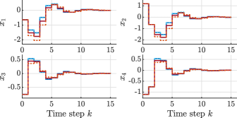
Figure 1: Simulated response of the LPV system in closed-loop with the controllers obtained using the model-based synthesis method (Stabilizing controller: , Quadratic performance controller: ) and our data-driven synthesis method (Stabilizing controller: , Quadratic performance controller: ).

This shows that our data-driven synthesis method, which only uses the measured data-set $\mathcal{D}_{N_{\mathrm{d}}}$ for the controller synthesis, is truly a counterpart of the model-based synthesis methods.

6.2.3 Quadratic perf. state-feedback LPV controller

Next, we design a data-driven state-feedback LPV controller that ensures quadratic performance using the developed tools in Theorem 4, using only the information in $\mathcal{D}_{N_{\mathrm{d}}}$. We choose $Q=I_{4}$ and $R=1$ for the performance objective (31). We solve the LMIs of Theorem 4 as an SDP on the vertices of $\mathbb{P}$, where we choose the objective function as $\max\mathrm{trace}(Z)$, which yields an LPV controller of the form (5), with

$$K_{0} =\begin{bmatrix}-0.0989&0.0878&-0.3018&-0.2412\end{bmatrix},$$ (41)

$$K_{1} =\begin{bmatrix}-0.2043&0.1308&-0.0349&-0.2645\end{bmatrix},$$

$$K_{2} =\begin{bmatrix}-0.0963&0.0593&-0.0123&-0.1767\end{bmatrix},$$

and $\mathrm{trace}(Z)=0.9151$. Again, we compare this result with a model-based synthesis approach, see [41, Prop. 1] using a constant Lyapunov matrix. The model-based controller synthesis yields

$$K_{0}^{\mathrm{m}} =\begin{bmatrix}-0.0082&0.0332&-0.2916&-0.1401\end{bmatrix},$$ (42)

$$K_{1}^{\mathrm{m}} =\begin{bmatrix}-0.1081&0.0676&-0.0002&-0.1353\end{bmatrix},$$

$$K_{2}^{\mathrm{m}} =\begin{bmatrix}0.0062&-0.0026&-0.0116&0.0088\end{bmatrix},$$

and $\mathrm{trace}(Z^{\mathrm{m}})=0.7146$.

We compare the model-based controller to the direct data-driven LPV controller via simulation, and the computation of the $\mathcal{H}^{\mathrm{g}}_{2}$-norm of the generalized plant in closed-loop for both controllers over an equidistant grid of 250 points over $\mathbb{P}$. The simulation results are given in Fig. 1, which shows that both controllers have a similar performance. The maximum of the achieved $\mathcal{H}^{\mathrm{g}}_{2}$-norm over the grid can be seen as an approximation of the ‘true’ $\mathcal{H}^{\mathrm{g}}_{2}$-norm of the LPV system. The resulting values for the data-based and the model-based controller are $5.27$ and $5.79$, respectively, which indicates that both controllers are very similar in terms of achieved performance. The difference between the two values is attributed to numerical differences during the solution of the problems.

From this example, we can conclude that the proposed data-driven control synthesis machinery provides competitive controllers w.r.t. model-based approaches by using only a few data samples measured from the system, rather than a full model. This considerably simplifies the overall LPV modeling and control toolchain, avoiding the two-step process of obtaining a model and then designing a model-based controller and respecting the control performance objectives in exploitation of the data. Moreover, it can cope with $p$-dependence of the $B$ matrix of the plant dynamics.

6.3 Application on the nonlinear unbalanced disc system

To demonstrate applicability of the proposed data-driven control on a real-world unstable nonlinear system, we consider the unbalanced disc setup, depicted in Fig. 2. This system consists of a DC motor that is connected to a disc containing an off-centered mass. Thus, the system behavior mimics the behavior of a rotational pendulum.

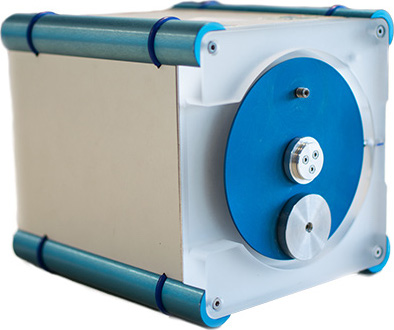
Figure 2: Unbalanced disc system, whose simulation model is used in Example 6.3.

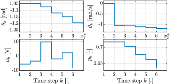
Figure 3: Data-dictionary $\mathcal{D}_{N_{\mathrm{d}}}$ consisting of 6 input-state-scheduling samples and an additional state-advancement ($x_{i}^{+}$). The dictionary is generated by simulating the unbalanced disc system with a random input sequence of 6 points and a random initial condition.

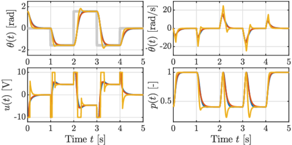
Figure 4: Simulation results of the unbalanced disc setup. The controllers track the reference signal ( ) for the angular position $\theta$ of the disc. The plots show the simulation response with Controller 1 ( ), Controller 2 ( ) and Controller 3 ( ).

6.3.1 System dynamics and data-generation

The nonlinear dynamics can be represented by the differential equation:

$$\ddot{\theta}(t)=-\frac{mgl}{J}\sin(\theta(t))-\frac{1}{\tau}\dot{\theta}+\frac{K_{\mathrm{m}}}{\tau}u(t),$$ (43)

where $\theta$ is the angular position of the disc, $u$ is the input voltage to the system, which is its control input, and $m,g,l,J,\tau,K_{\mathrm{m}}$ are the physical parameters of the system.

Table 1: Parameters of the unbalanced disc.

Parameter ​​​	$g$	$J$	​​​ $K_{\mathrm{m}}$​​​	$l$	$m$ ​​	​​ $\tau$ ​​	​​ $T_{\mathrm{s}}$ ​​
Value	$9.8$	​​​$2.2\!\cdot\!10^{\scalebox{0.65}[1.0]{$\,-$}4}$​​​	​​​$15.3$ ​​​	​​​$0.42$​​​	​​​$0.07$ ​​	​​ $0.6$ ​​	​​ $75$ ​​
Unit	​​​$[\mathrm{m}\!\cdot\!\mathrm{s}^{\scalebox{0.65}[1.0]{$\,-$}2}]$​​​	$[\mathrm{Nm}^{2}]$	$[\scalebox{0.65}[1.0]{$\,-$}]$	​​​$[\mathrm{mm}]$ ​​	​​ $[\mathrm{kg}]$ ​​	​​ $[\scalebox{0.65}[1.0]{$\,-$}]$ ​​	​​ $[\mathrm{ms}]$ ​​

In this work, we use the physical parameters of a real setup, as given in Table 1, which have been identified in [42] based on measurements from the real system. It is worth mentioning that this model has been considered for LPV control design, with successful implementation on the real hardware in [43]. Embedding (43) as an LPV system can be established by defining the scheduling signal as $p(t)=\mathrm{sinc}(\theta(t))=\tfrac{\sin(\theta(t))}{\theta(t)}$, from which we can immediately define $\mathbb{P}$ as $[-0.22,\;1]$. For a better formulation of the LFRs, we scaled $p$ such that $\mathbb{P}:=[-1,\;1]$.

For the data generation, we have implemented the nonlinear dynamical equations (43) in Matlab, which are solved using an ODE45 solver at a fixed sampling time of $T_{\mathrm{s}}=0.01$. By Condition 1, we need at least ${N_{\mathrm{d}}}=6$ data points. Hence, $\mathcal{D}_{N_{\mathrm{d}}}$ is generated by exciting the system with a uniform randomly generated input of length 6, where $u$ is in the range $[-10,\,10]$. Moreover, as it is assumed throughout the paper, the state measurements are noise-free. A posteriori, the scheduling $p$ is determined using the aforementioned scheduling map, with which $\mathcal{G}$ is constructed. The obtained data-dictionary $\mathcal{D}_{N_{\mathrm{d}}}$ that we use to synthesize the controllers is shown in Fig. 4. Note that we also depicted $\overrightarrow{X}$ in the upper plots of Fig. 4 by means of an additional state sample. For the obtained data-set, Condition 1 is verified, as $\mathrm{rank}(\mathcal{G})=6$.

6.3.2 Controller synthesis

We now use only the data in $\mathcal{D}_{N_{\mathrm{d}}}$ to synthesize LPV state-feedback controllers for the unbalanced disc system. Using our developed results in Theorems 4, 5 and 6, we synthesize three LPV state-feedback controllers for optimal 1) quadratic, 2) $\mathcal{H}^{\mathrm{g}}_{2}$-norm and 3) $\ell_{2}$-gain performance. Our objective is to regulate the states fast and smoothly to predefined operating points using a reasonable control input. In order to achieve this objective, we have tuned the matrices $Q$ and $R$ for the design problems 1, 2 and 3 as follows:

$$Q_{1} =Q_{2}=Q_{3}=\begin{bmatrix}8&0\\ 0&0.1\end{bmatrix}$$ (44a)

$$R_{1} =0.5,\ \ R_{2}=0.05,\ \ R_{3}=0.005.$$ (44b)

which have yielded controllers with relatively similar performance. As in the previous examples, the cost function for Controller 1 is chosen as $\max\mathrm{trace}(Z)$, while for Controller 2 we minimize the $\mathcal{H}^{\mathrm{g}}_{2}$-norm $\gamma$ during synthesis. In order to limit the aggressiveness of Controller 3, we modified the cost-function in the synthesis problem to $\min\gamma+\lambda\,\mathrm{trace}(Z)$, similar to the implementation of hinflmi in Matlab. Note that a $\lambda>0$ results in larger values of $\gamma$, i.e., the problem is regularized at the cost of performance. We choose $\lambda=0.1$. The results of the LPV controller synthesis problems are given in Table 2.

Table 2: Synthesis results.

	$\gamma$	$\mathcal{H}^{\mathrm{g}}_{2}\vphantom{\Big{)}}$-norm	$\ell_{2}$-gain
Controller 1	N/A	18.6	92.0
Controller 2	11.6	11.6	54.7
Controller 3	36.0	13.6	35.6

Additionally, we computed the maximum $\mathcal{H}_{2}$-norm and $\mathcal{H}_{\infty}$-norm of the resulting local LTI systems of the closed-loop LPV plant over a grid of $\mathbb{P}$. These results are given in Table 2 as well, and show that for Controllers 2 and 3 the guaranteed performance by the data-based synthesis is (approximately) equivalent to the resulting closed-loop performance.

6.3.3 Simulation results

Finally, the synthesized LPV controllers are applied on the original nonlinear model, where the control signal $u_{k}$ is applied to the continuous-time system in a zero-order-hold setting. Note that, by the considered state-feedback configuration, the controllers are designed for setpoint control of the origin. To show the capabilities of the controllers, we tested them in setpoint control of different forced equilibrium points $(x_{\mathrm{ss}},u_{\mathrm{ss}})$, as in [43]. In order to define the forced equilibrium points, the corresponding input steady-state values $u_{\mathrm{ss}}$ are calculated and added to the control law, which yields $u_{k}=K(p_{k})(x_{k}-x_{\mathrm{ss}})-u_{\mathrm{ss}}$. We chose to switch between $x_{\mathrm{ss}}=\{[0\ 0]^{\top}\!\!,\,[\tfrac{\pi}{2}\ 0]^{\top}\!\!,\,[-\tfrac{\pi}{2}\ 0]^{\top}\}$, where $x_{\mathrm{ss}_{1}}=\theta_{\mathrm{ss}}$ and $x_{\mathrm{ss}_{2}}=\dot{\theta}_{\mathrm{ss}}$. The simulation results are shown in Fig. 4. The aggressiveness of the $\ell_{2}$-gain performance-based controller can be explained by the choice of $R=0.005$, i.e., the cost on input is mild. In general, the designed controllers provide highly competitive performance, also when compared to the model-based results in [43, Fig. 6].

From this example, we can conclude that our proposed methods allow to synthesize LPV state-feedback controllers using only data, which can guarantee stability and performance of the closed-loop systems, even when the plant is a nonlinear system. Furthermore, in most cases, one will only need $(1+n_{\mathrm{p}})(n_{\mathrm{x}}+n_{\mathrm{u}})$ data-points measured from the nonlinear system, to be able to synthesize an LPV state-feedback controller.

7 Conclusion

In this work, we have derived novel direct data-driven methods that are capable of synthesizing LPV state-feedback controllers by only using information about the to-be-controlled system in the form of a persistently exciting data-set. Formulation of these results is made possible by the proposed data-driven representations of the open-loop and closed-loop behavior of the unknown LPV system. When the LPV state-feedback controllers, provided by the introduced synthesis algorithms, are connected to the unknown data-generating system, stability and performance of the closed-loop operation is guaranteed. By means of the presented examples, we demonstrate that our methods can achieve, based on only the measurement data, the same control performance as their model-based counterparts, while the latter uses perfect model knowledge of the system. Furthermore, we have demonstrated that, in line with the LPV embedding principle, the design methods can also be used for controlling nonlinear systems. We believe that our novel results can be the foundation for building a direct data-driven control framework for nonlinear systems with stability and performance guarantees. As a future work, we aim at the extension of the synthesis methods and the guarantees for noisy data-sets.

.1 Full-block $\mathcal{S}$-Procedure

For completeness, we give the known lemma from [44] on the full-block $\mathcal{S}$-procedure below. This result is instrumental and is used extensively throughout the paper.

Lemma .1.1 (Full-block $\mathcal{S}$-procedure [44]).

Given a quadratic matrix inequality

$$L^{\top}(p)WL(p)<0,\quad\forall p\in\mathbb{P},$$ (45)

with $L(p)=\Delta_{p}\star\bar{L}=L_{22}+L_{21}\Delta_{p}(I-L_{11}\Delta_{p})^{-1}L_{12}$, where

$$\Delta_{p}=\mathrm{diag}\big{\{}p_{1}I_{n_{\Delta 1}},\ p_{2}I_{n_{\Delta 2}},\cdots,p_{n_{\mathrm{p}}}I_{n_{\Delta n_{\mathrm{p}}}}\big{\}},$$ (46)

and $\mathbb{P}$ is convex, then (45) holds if and only if there exists a real full-block multiplier $\Xi=\Xi^{\top}$ defined as $\Xi=\begin{bmatrix}\Xi_{11}&\Xi_{12}\\ \Xi_{21}&\Xi_{22}\end{bmatrix}$, with $\Xi_{22}\succ 0$, such that

$$\left[\begin{array}[]{c}*\\ \hline\cr*\end{array}\right]^{\top}\left[\begin{array}[]{c|c}\Xi&0\\ \hline\cr 0&W\end{array}\right]\left[\begin{array}[]{c c}L_{11}&L_{12}\\ I&0\\ \hline\cr L_{21}&L_{22}\end{array}\right]\prec 0,$$ (47h)

$$\left[\begin{array}[]{c}*\\ \hline\cr*\end{array}\right]^{\top}\Xi\left[\begin{array}[]{c}I\\ \hline\cr\Delta_{p}\end{array}\right]\succeq 0,\quad\forall p\in\mathbb{P}.$$ (47m)

.2 Model-based LPV state-feedback control

In this section, the preliminaries for the proposed data-driven methods are discussed in terms of model-based LPV stability and performance analysis, followed by LPV state-feedback controller synthesis.

.2.1 Stabilizing control

Asymptotic stability of the LPV system (2), i.e., boundedness and convergence of the state-trajectories to the origin under $u\equiv 0$, is guaranteed with the existence of a Lyapunov function $V(x,p)=x^{\top}Z(p)x\succ 0$ with symmetric $Z:\mathbb{P}\rightarrow\mathbb{R}^{n_{\mathrm{x}}\times n_{\mathrm{x}}}$ that satisfies $V(x_{k+1},p_{k+1})-V(x_{k},p_{k})<0$ under all $(x,p,0)\in\mathfrak{B}$.

In the remainder, we perform the analysis on the closed-loop system (6). Stability of the closed-loop system can be verified with the following lemma:

Lemma .2.1 (Stabilizing LPV state-feedback [45]).

The controller $K$ in (5) asymptotically stabilizes (2) if there exists a symmetric $Z:\mathbb{P}\rightarrow\mathbb{R}^{n_{\mathrm{x}}\times n_{\mathrm{x}}}$ affine in $p$ such that

$$\begin{bmatrix}Z(p)&(*)^{\top}\\ A_{\textsc{CL}}(p)Z(p)&Z(p^{+})\end{bmatrix} \succ 0,$$ (48a)

$$Z(p) \succ 0,$$ (48b)

for all $p,p^{+}\in\mathbb{P}$, with $A_{\textsc{CL}}(p)$ as defined in (6), and $p^{+}$ is the time-shift of $p$, i.e., for $p_{k}$, $p^{+}=p_{k+1}$.

Proof.

We give it here for completeness, see also [45]. If (48b) holds, then $V(x,p)=x^{\top}\tilde{Z}(p)x\succ 0$ with $Z(p)=\tilde{Z}^{-1}(p)$ is true for all $(x,p)\in\mathfrak{B}_{\textsc{CL}}$, where

$$\mathfrak{B}_{\textsc{CL}}=\{(x,p)\mid(x,p,K(p)x)\in\mathfrak{B}\}.$$

Furthermore, (48a) under (48b) is equivalent with

$$A_{\textsc{CL}}^{\top}(p)\tilde{Z}(p^{+})A_{\textsc{CL}}(p)-\tilde{Z}(p)\prec 0,\quad\forall p,p^{+}\in\mathbb{P},$$

in terms of the Schur complement. This implies that $V(x^{+},p^{+})-V(x,p)<0$ for all vectors $p,p^{+}\in\mathbb{P}$ and $x\in\mathbb{R}^{n_{\mathrm{x}}}$ and hence under all $(x,p)\in\mathfrak{B}_{\textsc{CL}}$. Based on the fact that asymptotic stability of (6) is equivalent with the existence of a quadratic Lyapunov function fulfilling the above conditions [45]. ∎

As it is often done in the literature, in the sequel for conditions such as (48), we will use notation like $p$ for both the scheduling signal $p:\mathbb{Z}\rightarrow\mathbb{P}$ and for constant vectors $p\in\mathbb{P}$ to describe all possible values $p_{k}$, i.e., the value of the signal $p$ at time moment $k\in\mathbb{Z}$ can take. Where possible confusion might arise, we will clarify in the text which notion we refer to.

.2.2 Optimal quadratic performance

Beyond stability, design of a controller (5) can be used to ensure performance specifications on the closed-loop behavior. Performance of (6) can be expressed in various forms, such as the quadratic infinite-time horizon cost in (31). The following condition can be used to test whether a given $K$ stabilizes (2) and achieves the smallest possible bound on (31) under all $p\in\mathbb{P}^{\mathbb{Z}}$, i.e., achieves a minimal $\sup_{(x,p)\in\mathfrak{B}_{\textsc{CL}}}J(x,K(p)x)$.

Lemma .2.2 (Optimal quadratic perf. LPV state-feedback [31]).

The controller $K$ in (5) asymptotically stabilizes (2) and achieves the minimum of $\sup_{(x,p)\in\mathfrak{B}_{\textsc{CL}}}J(x,K(p)x)$, if $\sup_{p\in\mathbb{P}}\mathrm{trace}(Z(p))$ with $Z$ symmetric is minimal among all possible choices of $Z,K:\mathbb{P}\rightarrow\mathbb{R}^{n_{\mathrm{x}}\times n_{\mathrm{x}}}$ that satisfy

$$\begin{bmatrix}Z(p)&(*)^{\top}&(*)^{\top}&(*)^{\top}\\ A_{\textsc{CL}}(p)Z(p)&Z(p^{+})&0&0\\ Q^{\frac{1}{2}}Z(p)&0&I_{n_{\mathrm{x}}}&0\\ R^{\frac{1}{2}}K(p)Z(p)&0&0&I_{n_{\mathrm{u}}}\end{bmatrix} \succ 0,$$ (49a)

$$Z(p) \succ 0,$$ (49b)

for all $p,p^{+}\in\mathbb{P}$.

Proof.

If there exists a quadratic Lyapunov function $V(k):=x_{k}^{\top}\tilde{Z}(p_{k})x_{k}>0$, with $\tilde{Z}(p_{k})\succ 0$ for all $p_{k}\in\mathbb{P}$, such that

$$V(k+1)-V(k)\leq-(x_{k}^{\top}Qx_{k}+u_{k}^{\top}Ru_{k}),\quad\forall p_{k}\in\mathbb{P}$$ (50)

with $u_{k}=K(p_{k})x_{k}$ then, as the right-hand side is negative semidefinite due to $Q\succeq 0,R\succ 0$, $K$ is an asymptotically stabilizing controller for the LPV system (2), ensuring that $x_{k}\to 0$ as $k\to\infty$. Rewriting (50), we get

$$x_{k+1}^{\top}\tilde{Z}(p_{k+1})x_{k+1}-x_{k}^{\top}\tilde{Z}(p_{k})x_{k}\\ \leq-x_{k}^{\top}\left(Q+K^{\top}(p_{k})RK(p_{k})\right)x_{k}.$$ (51)

Summing all terms from 0 to $\infty$ yields

$$\sum_{k=1}^{\infty}x_{k+1}^{\top}\tilde{Z}(p_{k+1})x_{k+1}-x_{k}^{\top}\tilde{Z}(p_{k})x_{k}\leq-J(x,K(p)x).$$

If (51) holds, then, in terms of (50), $x_{k}\to 0$ as $k\to\infty$, and the telescopic sum on the left-hand side of the inequality reduces to $-x_{0}^{\top}\tilde{Z}(p_{0})x_{0}$, i.e., $x_{0}^{\top}\tilde{Z}(p_{0})x_{0}\geq J(x,K(p)x)$. Hence, $x_{0}^{\top}\tilde{Z}(p_{0})x_{0}$ is an upper bound on $J$, given that (51) holds. Inequality (51) is implied by

$$A_{\textsc{CL}}^{\top}(p)\tilde{Z}(p^{+})A_{\textsc{CL}}(p)-\tilde{Z}(p)+Q+K^{\top}(p)RK(p)\preccurlyeq 0,$$ (52)

holds for all $p,p^{+}\in\mathbb{P}$. Then, minimizing $J$ over all possible state and scheduling trajectories, i.e., $\sup_{(x,p)\in\mathfrak{B}_{\textsc{CL}}}J(x,K(p)x)$, can be rewritten as

$$\operatorname*{minimize}_{\tilde{Z},K} \quad x_{0}^{\top}\tilde{Z}(p_{0})x_{0}$$ (53a)

s.t. $$\quad\forall p,p^{+}\in\mathbb{P}:\tilde{Z}(p)\succ 0\text{ and \eqref{eq:pf:lqr2} holds},$$ (53b)

for all possible initial conditions $x_{0}\in\mathbb{R}^{n_{\mathrm{x}}}$ and $p_{0}\in\mathbb{P}$. By using the eigendecomposition of $\tilde{Z}(p)$, (53) is equivalent with minimizing $\mathrm{trace}(\tilde{Z}(p))$ subject to (53b) over all $p\in\mathbb{P}$. Moreover, applying the Schur complement on (52) w.r.t. $\mathrm{blkdiag}(\tilde{Z}(p^{+}),I_{n_{\mathrm{x}}},I_{n_{\mathrm{u}}})$, followed by a congruence transformation $\mathrm{blkdiag}(Z(p),I_{n_{\mathrm{x}}},I_{n_{\mathrm{x}}},I_{n_{\mathrm{u}}})$ on the resulting matrix inequality, where $Z(p)=\tilde{Z}^{-1}(p)$, yields

$$\operatorname*{minimize}_{Z,K} \quad\sup_{p\in\mathbb{P}}\ \mathrm{trace}(Z(p))$$

s.t. $$\quad\forall p,p^{+}\in\mathbb{P}:\text{ \eqref{eq:LQR-LPV-model-based} holds,}$$

completing the proof. ∎

.2.3 $\mathcal{H}^{\mathrm{g}}_{2}$ performance

In order to consider induced gains based performance metrics, such as the extended $\mathcal{H}_{2}$ performance, widely used in linear control, we will introduce a representation of general controller configurations in terms of the generalized plant concept. Consider the following LPV formulation of the plant to be controlled with state-feedback

$$x_{k+1} =A(p_{k})x_{k}+B(p_{k})u_{k}+B_{\mathrm{w}}(p_{k})w_{k},$$ (54a)

$$y_{k} =x_{k}$$ (54b)

$$z_{k} =C_{\mathrm{z}}(p_{k})x_{k}+D_{\mathrm{zu}}(p_{k})u_{k}+D_{\mathrm{zw}}(p_{k})w_{k},$$ (54c)

where $w_{k}\in\mathbb{R}^{n_{\mathrm{w}}}$ is a signal being the collection of generalized disturbances, such as reference signals, load disturbances, etc., while $z_{k}\in\mathbb{R}^{n_{\mathrm{w}}}$ is the generalized performance signal, being the collection of control objectives, such as tracking error or input usage. $y_{k}=x_{k}$ expresses that the observed outputs of the plant are available for the controller, which is in line with the considered state-feedback objective. To avoid complexity by using performance shaping filters and to be compatible with the considered quadratic performance concept in (31), consider

$$C_{\mathrm{z}} =\begin{bmatrix}Q^{\frac{1}{2}}\\ 0\end{bmatrix}, D_{\mathrm{zu}}=\begin{bmatrix}0\\ R^{\frac{1}{2}}\end{bmatrix},\quad D_{\mathrm{zw}}=0.$$ (55a)

This implies that $w_{k}\in\mathbb{R}^{n_{\mathrm{x}}}$ and $z_{k}\in\mathbb{R}^{n_{\mathrm{x}}+n_{\mathrm{u}}}$. Closing the loop with feedback law (5), yields the closed-loop system (33).

Using the definition of the $\mathcal{H}^{\mathrm{g}}_{2}$-norm in (34), the following lemma, which is a slight modification of [33, Lem. 1], allows to find a bound $\gamma$ on the $\mathcal{H}^{\mathrm{g}}_{2}$-norm of the closed-loop system and guarantee stability of (33).

Lemma .2.3 ($\mathcal{H}^{\mathrm{g}}_{2}$-norm perf. LPV state-feedback).

The controller $K$ in (5) asymptotically stabilizes (2) and achieves an $\mathcal{H}^{\mathrm{g}}_{2}$-norm of (33) that is less than a given $\gamma>0$, if there exist symmetric matrices $Z:\mathbb{P}\rightarrow\mathbb{R}^{n_{\mathrm{x}}\times n_{\mathrm{x}}}$ and $S\in\mathbb{R}^{n_{\mathrm{u}}\times n_{\mathrm{u}}}$ such that

$$\begin{bmatrix}Z(p^{+})-I_{n_{\mathrm{x}}}&A_{\textsc{CL}}(p)Z(p)\\ (\ast)^{\top}&Z(p)\end{bmatrix} \succ 0,$$ (56a)

$$\begin{bmatrix}S&R^{\frac{1}{2}}K(p)Z(p)\\ (\ast)^{\top}&Z(p)\end{bmatrix} \succ 0,$$ (56b)

$$\mathrm{trace}(Q{Z}(p))+\mathrm{trace}(S) \prec\gamma^{2},$$ (56c)

for all $p,p^{+}\in\mathbb{P}$.

Proof.

Applying the result of [33, Lem. 1] to (33), denoted by $\Sigma_{\textsc{CL}}$, the $\mathcal{H}^{\mathrm{g}}_{2}$-norm can be written as

$$\|\Sigma_{\textsc{CL}}\|_{\mathcal{H}^{\mathrm{g}}_{2}}^{2}=\limsup_{N\to\infty}\tfrac{1}{N}\!\sum_{k=0}^{N}\mathrm{trace}\left(C(p_{k})\bar{Z}(p_{k})C^{\top}(p_{k})\right),$$ (57)

where $\bar{Z}(p_{k})$ is the controllability Gramian that satisfies

$$A_{\textsc{CL}}(p_{k})\bar{Z}(p_{k})A_{\textsc{CL}}^{\top}(p_{k})-\bar{Z}(p_{k+1})+I_{n_{\mathrm{x}}}=0$$ (58)

with $\bar{Z}(p_{0})=0$. Inequality (56a) implies that ${Z}(p)\succ 0$ and

$$A_{\textsc{CL}}(p){Z}(p)A_{\textsc{CL}}^{\top}(p)-{Z}(p^{+})+I_{n_{\mathrm{x}}}\prec 0,$$ (59)

which ensures asymptotic stability of (33). Furthermore, there exists a $W(p)=W^{\top}(p)\succ 0$ such that

$$A_{\textsc{CL}}(p){Z}(p)A_{\textsc{CL}}^{\top}(p)-{Z}(p^{+})+I_{n_{\mathrm{x}}}+W(p)=0,$$ (60)

which implies (58) for all $k\geq 0$ with $Z\succ\bar{Z}$. Moreover, (56b) implies that

$$S\succ R^{\frac{1}{2}}K(p)Z(p)K^{\top}(p)R^{\frac{\top}{2}}.$$ (61)

Substituting the latter in (56c) gives

$$\mathrm{trace}(QZ(p))+\mathrm{trace}(S)>\\ \mathrm{trace}(QZ(p))+\mathrm{trace}(R^{\frac{1}{2}}K(p)Z(p)K^{\top}(p)R^{\frac{\top}{2}}),$$ (62)

where the right-hand side can be rewritten using the cyclic property of the trace as

$$\mathrm{trace}(C(p)Z(p)C^{\top}(p)),$$ (63)

with $C(p)=\begin{bmatrix}(Q^{\frac{1}{2}})^{\top}&(R^{\frac{1}{2}}K(p_{k}))^{\top}\end{bmatrix}^{\top}$. Hence, finding a $\gamma$ for which (56) holds for all $p\in\mathbb{P}$ ensures via (56c) that (57) is upper bounded by $\gamma$, concluding the proof. ∎

.2.4 $\ell_{2}$-gain performance

The (induced) $\ell_{2}$-gain, as introduced in Section 5.3, can be seen as the ‘generalization’ of the $\mathcal{H}_{\infty}$ norm to the LPV case and is a widely used performance metric in model-based LPV control. The following result allows to analyze stability and $\ell_{2}$-gain performance of the closed-loop system (33).

Lemma .2.4 ($\ell_{2}$-gain perf. LPV state-feedback).

The controller $K$ in (5) asymptotically stabilizes (2) and achieves an $\ell_{2}$-gain of (33) that is less than a given $\gamma>0$, if there exists a symmetric matrix $Z:\mathbb{P}\rightarrow\mathbb{R}^{n_{\mathrm{x}}\times n_{\mathrm{x}}}$ such that

$$\begin{bmatrix}Z(p)&(*)^{\top}&(*)^{\top}&(*)^{\top}&0\\ A_{\textsc{CL}}(p){Z}(p)&Z(p^{+})&0&0&I_{n_{\mathrm{x}}}\\ Q^{\frac{1}{2}}Z(p)&0&\gamma I_{n_{\mathrm{x}}}&0&0\\ R^{\frac{1}{2}}K(p)Z(p)&0&0&\gamma I_{n_{\mathrm{u}}}&0\\ 0&I_{n_{\mathrm{x}}}&0&0&\gamma I_{n_{\mathrm{x}}}\end{bmatrix} \succ 0,$$ (64a)

$${Z}(p) \succ 0,$$ (64b)

for all $p,p^{+}\in\mathbb{P}$.

Proof.

Following standard formulation, e.g., [35], for $\ell_{2}$-gain performance for the closed-loop LPV system (33), the following condition should hold for all $p,p^{+}\in\mathbb{P}$:

$$\begin{bmatrix}(*)^{\top}\tilde{Z}(p^{+})A_{\textsc{CL}}(p)-\tilde{Z}(p)&(*)^{\top}\\ \tilde{Z}(p^{+})A_{\textsc{CL}}(p)&\tilde{Z}(p^{+})-\gamma I_{n_{\mathrm{x}}}\end{bmatrix}\\ +\frac{1}{\gamma}\begin{bmatrix}*\end{bmatrix}^{\top}\begin{bmatrix}Q^{\frac{1}{2}}&0\\ R^{\frac{1}{2}}K(p)&0\end{bmatrix}\prec 0$$

with $\tilde{Z}^{\top}(p)=\tilde{Z}(p)\succ 0$. The above matrix inequality can be rewritten as

$$0\prec\begin{bmatrix}\tilde{Z}(p)&0\\ 0&\gamma I_{n_{\mathrm{x}}}\end{bmatrix}-\\ \begin{bmatrix}*\end{bmatrix}^{\top}\begin{bmatrix}\tilde{Z}^{-1}(p^{+})&0&0\\ 0&\tfrac{1}{\gamma}I_{n_{\mathrm{x}}}&0\\ 0&0&\tfrac{1}{\gamma}I_{n_{\mathrm{u}}}\end{bmatrix}\begin{bmatrix}\tilde{Z}(p^{+})A_{\textsc{CL}}(p)&\tilde{Z}(p^{+})\\ Q^{\frac{1}{2}}&0\\ R^{\frac{1}{2}}K(p)&0\end{bmatrix}.$$

Now, applying the Schur complement with respect to $\mathrm{blkdiag}(\tilde{Z}^{-1}(p^{+}),\tfrac{1}{\gamma}I_{n_{\mathrm{x}}},\tfrac{1}{\gamma}I_{n_{\mathrm{u}}})$ and the congruence transformation $\mathrm{blkdiag}({Z}(p),I_{n_{\mathrm{x}}},{Z}(p^{+}),I_{n_{\mathrm{x}}},I_{n_{\mathrm{u}}})$ on the resulting matrix inequality, where $Z(p)=\tilde{Z}^{-1}(p)$, yields the condition

$$\begin{bmatrix}Z(p)&0&(*)^{\top}&(*)^{\top}&(*)^{\top}\\ 0&\gamma I_{n_{\mathrm{x}}}&I_{n_{\mathrm{x}}}&0&0\\ A_{\textsc{CL}}(p){Z}(p)&I_{n_{\mathrm{x}}}&Z(p^{+})&0&0\\ Q^{\frac{1}{2}}Z(p)&0&0&\gamma I_{n_{\mathrm{x}}}&0\\ R^{\frac{1}{2}}K(p)Z(p)&0&0&0&\gamma I_{n_{\mathrm{u}}}\end{bmatrix}\succ 0.$$

Finally, pre- and post-multiplication of the above matrix inequality by the permutation matrix

$$P=\begin{bmatrix}I_{n_{\mathrm{x}}}&0&0&0&0\\ 0&0&0&0&I_{n_{\mathrm{x}}}\\ 0&I_{n_{\mathrm{x}}}&0&0&0\\ 0&0&I_{n_{\mathrm{x}}}&0&0\\ 0&0&0&I_{n_{\mathrm{u}}}&0\\ \end{bmatrix}$$

and its transpose, respectively, yields condition (64a). ∎

.2.5 Controller synthesis

When $K$ is not known, the matrix inequality conditions in Lemmas .2.1–.2.4 are nonlinear in the decision variables (controller parameters and Lyapunov functions) and provide an infinite number of inequalities that need to be satisfied for every point in $\mathbb{P}$. To resolve these problems and recast these conditions to tractable controller synthesis methods, the change of variables $Y(p)=K(p)Z(p)$ can be applied in the conditions (48a), (49a), (56a), (56b) and (64a). Furthermore, the dependence on $p$ must be defined for $K$ and ${Z}$ (i.e., for $Y(p)$), which has an important impact on the complexity of the synthesis problem and the achievable control performance. A natural choice for the scheduling dependence of $K$ is to assume static-affine dependence on $p$ as in (5b). On the other hand, the choice of the scheduling dependence of ${Z}$ is not trivial, as discussed in [46], and it is often accomplished in terms of the choice of $Y$. These considerations allow to convert the corresponding LPV state-feedback controller synthesis problems into the minimization of a linear cost, subject to constraints defined by an infinite set of LMIs. The last step in making the synthesis problems tractable is reducing the set of constraints to a finite number of LMIs, such that the resulting SDP problem can be solved using efficient solvers. There are multiple methods available to accomplish this. As can be seen in the main body of this paper, we use the full-block $\mathcal{S}$-procedure, see Appendix .1 to recast the synthesis problems to an SDP of finite size.

References

• [1] R. Tóth, Modeling and Identification of Linear Parameter-Varying Systems, 1st ed.   Springer-Verlag, 2010.
• [2] J. Mohammadpour and C. W. Scherer, Control of Linear Parameter Varying Systems with Applications.   Heidelberg: Springer, 2012.
• [3] A. A. Bachnas, R. Tóth, A. Mesbah, and J. Ludlage, “A review on data-driven linear parameter-varying modeling approaches: A high-purity distillation column case study,” Journal of Process Control, vol. 24, pp. 272–285, 2014.
• [4] P. B. Cox and R. Tóth, “Linear parameter-varying subspace identification: A unified framework,” Automatica, vol. 123, p. 109296, 2021.
• [5] Y. Bao and J. Mohammadpour Velni, “An overview of data-driven modeling and learning-based control design methods for nonlinear systems in LPV framework,” in Proc. of the 5th Workshop on Linear Parameter Varying Systems, 2022.
• [6] J. W. van Wingerden and M. Verhaegen, “Subspace identification of bilinear and LPV systems for open- and closed-loop data,” Automatica, vol. 45, no. 2, pp. 372–381, 2009.
• [7] P. L. dos Santos, C. Novara, D. Rivera, J. Ramos, and T. Perdicoúlis, editors, Linear Parameter-Varying System Identification: New Developments and Trends.   Singapore: World Scientific Publishing, 2011.
• [8] P. den Boef, P. B. Cox, and R. Tóth, “LPVcore: Matlab toolbox for LPV modelling, identification and control,” in Proc. of the 19th Symposium on System Identification, 2021.
• [9] J. Schoukens and L. Ljung, “Nonlinear system identification: A user-oriented road map,” IEEE Control Systems Magazine, vol. 39, no. 6, pp. 28–99, 2019.
• [10] M. Gevers, “Identification for control: From the early achievements to the revival of experiment design,” European Journal of Control, vol. 11, no. 4, pp. 335–352, 2005.
• [11] Z.-S. Hou and Z. Wang, “From model-based control to data-driven control: Survey, classification and perspective,” Information Sciences, vol. 235, pp. 3–35, 2013.
• [12] S. Formentin, D. Piga, R. Tóth, and S. M. Savaresi, “Direct learning of LPV controllers from data,” Automatica, vol. 65, pp. 98–110, 2016.
• [13] J. Miller and M. Sznaier, “Data-driven gain scheduling control of linear parameter-varying systems using quadratic matrix inequalities,” IEEE Control Systems Letters, vol. 7, pp. 835–840, 2022.
• [14] S. Yahagi and I. Kajiwara, “Direct data-driven tuning of look-up tables for feedback control systems,” IEEE Control Systems Letters, vol. 6, pp. 2966–2971, 2022.
• [15] J. C. Willems, P. Rapisarda, I. Markovsky, and B. L. De Moor, “A note on persistency of excitation,” Systems & Control Letters, vol. 54, no. 4, pp. 325–329, 2005.
• [16] I. Markovsky and P. Rapisarda, “Data-driven simulation and control,” International Journal of Control, vol. 81, no. 12, p. 1946–1959, 2008.
• [17] A. Romer, J. Berberich, J. Köhler, and F. Allgöwer, “One-shot verification of dissipativity properties from input–output data,” IEEE Control Systems Letters, vol. 3, no. 3, pp. 709–714, 2019.
• [18] A. Koch, J. Berberich, and F. Allgöwer, “Provably robust verification of dissipativity properties from data,” IEEE Transactions on Automatic Control, vol. 67, no. 8, pp. 4248–4255, 2021.
• [19] H. J. van Waarde, M. K. Camlibel, P. Rapisarda, and H. L. Trentelman, “Data-driven dissipativity analysis: Application of the matrix S-lemma,” IEEE Control Systems Magazine, vol. 42, pp. 140–149, 2022.
• [20] C. De Persis and P. Tesi, “Formulas for Data-Driven Control: Stabilization, Optimality, and Robustness,” IEEE Transactions on Automatic Control, vol. 65, no. 3, pp. 909–924, 2019.
• [21] J. Coulson, J. Lygeros, and F. Dörfler, “Data-enabled predictive control: In the shallows of the DeePC,” in Proc. of the European Control Conference, 2019, pp. 307–312.
• [22] J. Berberich, J. Köhler, M. A. Müller, and F. Allgöwer, “Data-driven model predictive control with stability and robustness guarantees,” IEEE Transactions on Automatic Control, vol. 66, no. 4, pp. 1702–1717, 2021.
• [23] C. Verhoek, R. Tóth, S. Haesaert, and A. Koch, “Fundamental Lemma for Data-Driven Analysis of Linear Parameter-Varying Systems,” in Proc. of the 60th IEEE Conference on Decision and Control, 2021.
• [24] C. Verhoek, H. S. Abbas, R. Tóth, and S. Haesaert, “Data-driven predictive control for linear parameter-varying systems,” in Proc. of the 4th Workshop on Linear Parameter Varying Systems, 2021.
• [25] C. Verhoek, J. Berberich, S. Haesaert, F. Allgöwer, and R. Tóth, “Data-driven dissipativity analysis of linear parameter-varying systems,” arXiv preprint arXiv:2303.10031, 2023.
• [26] R. A. Horn and C. R. Johnson, Topics in Matrix Analysis.   Cambridge University Press, 1991.
• [27] M. H. de Lange, C. Verhoek, V. Preda, and R. Tóth, “LPV modeling of the atmospheric flight dynamics of a generic parafoil return vehicle,” in Proc. of the 5th Workshop on Linear Parameter-Varying Systems, 2022.
• [28] R. Tóth, H. S. Abbas, and H. Werner, “On the state-space realization of LPV input-output models: Practical approaches,” IEEE Transactions on Control Systems Technology, vol. 20, no. 1, pp. 139–153, 2011.
• [29] P. B. Cox and R. Tóth, “Linear parameter-varying subspace identification: A unified framework,” Automatica, vol. 123, p. 109296, 2021.
• [30] C. Poussot-Vassal, P. Vuillemin, and C. Briat, “Non-intrusive nonlinear and parameter varying reduced order modelling,” in Proc. of the 4th Workshop on Linear Parameter Varying Systems, 2021.
• [31] D. Rotondo, V. Puig, and F. Nejjari, “Linear quadratic control of LPV systems using static and shifting specifications,” in Proc. of the European Control Conference, 2015, pp. 3085–3090.
• [32] R. L. Pereira, M. S. de Oliveira, and K. H. Kienitz, “Discrete-time $\mathcal{H}_{2}$ state-feedback control of polytopic LPV systems,” Optimal Control Applications and Methods, vol. 42, no. 4, pp. 1016–1029, 2021.
• [33] J. de Caigny, J. F. Camino, R. C. L. F. Oliveira, P. L. D. Peres, and J. Swevers, “Gain-scheduled $H_{2}$ and $H_{\infty}$ control of discrete-time polytopic time-varying systems,” IET Control Theory & Applications, vol. 4, no. 3, pp. 362–380, 2010.
• [34] A. J. van der Schaft, $\mathcal{L}_{2}$-Gain and Passivity Techniques in Nonlinear Control, 3rd ed., ser. Communications and Control Engineering.   Cham, Switzerland: Springer International Publishing, 2017.
• [35] P. Gahinet and P. Apkarian, “A linear matrix inequality approach to $H_{\infty}$ control,” International Journal of Robust and Nonlinear Control, vol. 4, pp. 421–428, 1994.
• [36] C. Verhoek, H. S. Abbas, and R. Tóth, “Direct data-driven LPV control of nonlinear systems: An experimental result,” in Proc. of the 22nd IFAC World Congress, 2023.
• [37] J. Löfberg, “YALMIP: A toolbox for modeling and optimization in Matlab,” in Proc. of the IEEE International Conference on Robotics and Automation, 2004, pp. 284–289.
• [38] MOSEK ApS. (2022) Mosek optimization toolbox (version 9.3). [Online]. Available: https://www.mosek.com
• [39] H. S. Abbas, G. Männel, C. Herzog né Hoffmann, and P. Rostalski, “Tube-based model predictive control for linear parameter-varying systems with bounded rate of parameter variation,” Automatica, vol. 107, no. 9, pp. 21–28, 2019.
• [40] A. Pandey and M. C. de Oliveira, “Quadratic and poly-quadratic discrete-time stabilizability of linear parameter-varying systems,” in Proc. of the 20th IFAC World Congress, 2017, pp. 8624–8629.
• [41] Y. Bao, H. S. Abbas, and J. M. Velni, “A learning-and scenario-based MPC design for nonlinear systems in LPV framework with safety and stability guarantees,” International Journal of Control, 2023.
• [42] P. J. W. Koelewijn and R. Tóth, “Physical parameter estimation of an unbalanced disc system,” Eindhoven University of Technology, Tech. Rep., 2019, TUE-CS-2019.
• [43] H. S. Abbas, R. Tóth, M. Petreczky, N. Meskin, J. Mohammadpour Velni, and P. J. W. Koelewijn, “Lpv modeling of nonlinear systems: A multi-path feedback linearization approach,” International Journal of Robust and Nonlinear Control, vol. 31, no. 18, pp. 9436–9465, 2021.
• [44] C. Scherer, “LPV control and full block multipliers,” Automatica, vol. 27, no. 3, pp. 325–485, 2001.
• [45] P. B. Cox, S. Weiland, and R. Tóth, “Affine parameter-dependent lyapunov functions for lpv systems with affine dependence,” IEEE Transactions on Automatic Control, vol. 63, no. 11, pp. 3865–3872, 2018.
• [46] P. Apkarian and R. Adams, “Advanced gain-scheduling techniques for uncertain systems,” IEEE Transactions on Control Systems Technology, vol. 6, no. 1, pp. 21–32, 1998.