Nonlinear Advantage: Trained Networks Might Not Be As Complex as You Think

Abstract

We perform an empirical study of the behaviour of deep networks when fully linearizing some of its feature channels through a sparsity prior on the overall number of nonlinear units in the network. In experiments on image classification and machine translation tasks, we investigate how much we can simplify the network function towards linearity before performance collapses. First, we observe a significant performance gap when reducing nonlinearity in the network function early on as opposed to late in training, in-line with recent observations on the time-evolution of the data-dependent NTK. Second, we find that after training, we are able to linearize a significant number of nonlinear units while maintaining a high performance, indicating that much of a network’s expressivity remains unused but helps gradient descent in early stages of training. To characterize the depth of the resulting partially linearized network, we introduce a measure called average path length, representing the average number of active nonlinearities encountered along a path in the network graph. Under sparsity pressure, we find that the remaining nonlinear units organize into distinct structures, forming core-networks of near constant effective depth and width, which in turn depend on task difficulty.

1 Introduction

Deep learning as such is based on the idea that concatenations of (suitably chosen) nonlinear functions increase expressivity so that complex pattern modeling and recognition problems can be solved. While initial approaches such as AlexNet (Krizhevsky et al., 2012) only used moderate depth, improvements such as batch normalization (Ioffe & Szegedy, 2015; Santurkar et al., 2018; Arora et al., 2019) or residual connections (He et al., 2015b) made the training of networks with hundreds or even thousands of layers possible, and this did contribute to significant practical gains.

From a theoretical perspective, a network’s depth (along with its width) upper bounds the complexity of the function that it can represent (Bartlett et al., 2019) and therefore upper bounds the network’s expressivity. Indeed, deeper networks tend to enhance performance (Tan & Le, 2019), but gains seem to taper off and saturate with increasing depth. Very deep networks are also known to be more difficult to analyze (Allen-Zhu et al., 2019), more computationally expensive to train or infer and suffer from numerous stability issues such as vanishing (Hochreiter, 1991), exploding (Zhang et al., 2019) and shattering (Balduzzi et al., 2017) gradients. Similar arguments can be made about layer width: a sufficiently large network can memorize any given function (Cybenko, 1989), but under standard initialization and training infinite width networks degrade to Gaussian processes (Jacot et al., 2018).

From a practical perspective, there are now many successful recipes for creating networks of a prescribed depth, but it is still difficult to understand – empirically or analytically – how many nonlinear layers and features per layer are actually needed to solve a problem, and how effective a chosen architecture actually is in exploiting its expressive potential in the sense of a deep stack of concatenated nonlinear computations.

Our paper addresses this question from an empirical perspective: we use a simple setup that associates every nonlinear unit with a cost at channel granularity, which can be raised continuously, while simultaneously trying to maintain performance. As PReLU activations (He et al., 2015a) can be used to interpolate continuously between a ReLU function and a linear function (Ali Mehmeti-Göpel et al., 2021), we replace each ReLU layer with channel-wise PReLU activations and regularize their slopes towards linearity. Such a linearized feature channel therefore only forms linear combinations of existing feature channels, thereby not effectively contributing to the nonlinear complexity of the network. To measure the nonlinear complexity or ”effective depth” of the resulting partially linearized networks, we introduce a metric called average path length (APL): the average amount of nonlinear units a given input traverses until it passes the final layer. We thereby disregard subsequent linear mappings along computational paths, as these do not increase expressivity in a nonlinear sense.

Using this tool, we make a series of experiments on common convolutional and transformer architectures on standard computer vision and machine translation tasks by partially linearizing networks with regard to the network’s inputs at different stages of training and find that networks linearized later on in training obtain a significantly higher performance than networks linearized earlier on in training. This is non-trivial, since the network’s expressivity is the same whether it is linearized early or late in training. We find the biggest differences in the early training phase, complementarily to the findings of (Fort et al., 2020) that establish a similar, but much less surprising effect when fully linearizing the network with regard to the network’s weights.

Analyzing these partially linearized networks extracted after training, we find that we can extract very shallow networks with a surprisingly high performance for their effective depth. These findings are consistent with the lottery ticket hypothesis (Frankle & Carbin, 2019) that there is a core nonlinear structure in networks, and with the subsequent findings of You et al. (2020) that it forms within the first epochs of training. Our method allows us to compute an approximate lower bound for depth and width that the networks needs to solve a task before performance collapses and we find that these are approximately constant for a given task and regularization strength, independently of the width and depth of the initial network. We also find that the effective depth of this core nonlinear structure grows with problem complexity for a fixed regularization strength.

2 Related Work and Contributions

Different approaches to network pruning were explored in recent years: magnitude-based weight pruning, weight-regularization techniques, sensitivity-based pruning and search-based approaches (Neill, 2020). Frankle & Carbin (2019) extract a highly performant, sparse and re-trainable subnetwork by removing all low-magnitude weights after a given training time, re-initializing the network and iterating this process. This motivates the ”lottery ticket hypothesis” of a network consisting of a smaller core structure embedded in the larger, overparametrized and redundant network, which, in their case, can be extracted by weight pruning. Our paper prunes nonlinear units instead of weights, but comes to similar findings of a problem-difficulty-dependent minimal set, embedded in a much larger and deeper network, when considering nested nonlinear computations. You et al. (2020) claim that the final accuracy of lottery tickets drawn after at early training is already drastically higher than at initialization. Su et al. (2020) conduct ”sanity checks” on the lottery ticket hypothesis and conclude that only the number of remaining weights matters for a given dataset. We conduct similar checks and find that transferring simple statistics such as how many nonlinear units are active per layer are not sufficient to recover full performance.

Simplification of networks by reducing nonlinearity has become a major area of interest. A lot of recent work has studied the neural tangent kernel (NTK) approximation, which linearizes the network function with regard to its parameters. It arises in the infinite width limit (under mild conditions) or by explicitly performing a linear Taylor-approximation of a finite network (Jacot et al., 2018; Fort et al., 2020). As it fully linearizes training, the NTK has been tremendously useful for gaining a better understanding of the training of deep network, such explaining double-descent generalization (Belkin et al., 2019; Wilson & Izmailov, 2020). Maybe unsurprisingly, linearized training hurts performance in practice (Fort et al., 2020) and theory: Roberts et al. (2022) attribute it to the loss of detection of higher-order moments in the data distribution). Fort et al. have coined the term nonlinear advantage for the observed discrepancy in performance between the network’s NTK and the nonlinear network function that vanishes over time when training with low learning rate. Within the NTK framework, the impact of ReLUs can be captured by path kernels (Lakshminarayanan & Singh, 2020), the learning of which improves results and generalizes when retraining, and can be used to understand pruning methods at initialization (Gebhart et al., 2021). Our APL measures are tightly related to the proposed (gated) path-integral formulation there. Our paper simplifies the network function itself by reducing the number of nonlinear units in the network and therefore partially linearizing it in both inputs and weights, finding a similar, but difficulty-dependent nonlinear advantage.

Dror et al. (2021) use a methodology similar to ours, but applied layer-wise and aiming at improved performance characteristics at inference time. Our channel-wise approach allows us to reduce significantly more nonlinear units in the network whilst maintaining a similar performance as well as characterize the ”effective width” of the emerging core network. A training time dependent effect as we show it, is not studied by the authors.

3 Reducing Nonlinear Feature Channels

In order to reduce the amount of nonlinear feature channels in a network, we take network architectures and replace their ReLU activations with PReLUs. We then use a single PReLU weight for every channel and add a sparsity regularization of $L_{0.5}=\sum|1-\alpha_{i}|^{0.5}$ to the regular training loss scaled with a regularization weight $\omega$, where $\alpha_{i}$ is the variable slope of the i-th PReLU. We chose channel-wise PReLU units because the latter allows a much bigger reduction in overall nonlinearity compared to layer-wise units, and pixel-wise PReLUs would entail an unreasonable amount of additional parameters. Since the regularization loss term is discontinuous at $1$, we disable a PReLU unit if their slope gets close enough to one. We call such a unit inactive, while all other units are active.

By regularizing PReLU units this way, the slope of inactive units is locked to $\alpha_{i}=1$, but the slope of active units is an arbitrary number between 0 and 1. After reaching a goal percentage of disabled PReLU units, it is possible to regularize the slope of the remaining active units back to 0, effectively transforming the network back to a regular ReLU network and relating to (Hanin & Rolnick, 2019), but we found that this method can be hurtful to performance and therefore refrain from using it.

3.1 Average Path Length (APL)

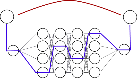
Figure 1: In this Figure, a residual connection (red) skips 4 small fully connected layers. The left-most and right-most nodes are connected by 257 different paths. Using unnormalized average path length implies a $1/257$ chance of selecting the red path and the same chance of selecting the blue path. Using normalized average path length, we have a $1/2$ chance of selecting the red path and a $1/512$ chance of selecting the blue path.

The depth of a network, according to its traditional notion, corresponds to the maximum amount of nonlinear units encountered when following the computation graph of a network from input to output. After partially linearizing such a network, this value remains the same, assuming at least one channel per layer remains active (non-linear). Therefore, computing the average amount of nonlinear units instead of the maximum seems like a more sensible characterization for partially linearized networks.

Let $G=(V,E)$ be the directed acyclic graph that represents the computation graph of a given feedforward neural network. Since we are only interested in the nonlinear structure of the graph, a node in the graph corresponds to a PReLU unit in the network. We denominate $V_{d}\subset V$ the subset of nodes that correspond to the $d$-th layer in the network. Let $v_{in},v_{out}\in V$ be the respective input and output vertices of the graph. Let $R\subset V$ be a subset of the vertices that represent the blocks containing an active PReLU i.e. $|\alpha-1|>\epsilon$, where $\alpha$ is the weight of the PReLU.

Let $\mathcal{P}^{(n)}\subset V^{n}$ be the set of all paths of length $n$ in $G$ that originate in $v_{in}$, i.e. $p_{1}\in v_{in}$ and $(v_{i},v_{i+1})\in E$ for all $1\leq i\leq n-1$. We define the effective path length of a path $p\in\mathcal{P}^{(n)}$ as the number of active PReLU activations it traverses:

$$\phi(p)\vcentcolon=|\{v_{i}\in p~{}|~{}v_{i}\in R,~{}1\leq i\leq n\}|,$$

which is always smaller or equal to its regular length $|p|$. Let $v\in V$ be a vertex of the graph, we then define its path histogram function as the number of paths from $v_{in}$ to $v$ of effective length $l$ :

$$\phi^{(l)}(v)\vcentcolon=|\{p\in\mathcal{P}^{(l^{\prime})}~{}|~{}p_{l}=v,~{}\phi(p)=l,~{}1\leq l^{\prime}\leq l\}|.$$

We finally define the average path length (APL) of the network as:

$$APL(G)\vcentcolon=\frac{\sum_{i=0}^{d}i\cdot\phi^{(i)}(v_{out})}{\sum_{i=0}^{d}\phi^{(i)}(v_{out})},$$

where $d$ is the depth of the network. In order to effectively compute the APL of a network, we resort to dynamic programming.

Proposition 3.1.

Let $v\in V$ be a vertex in the network. We can then compute its path histogram function by summing over all vertices that have an outgoing edge to $v$:

$\phi^{(l)}(v)=\begin{cases}\sum_{v^{\prime}\in V}\mathbbm{1}_{(v^{\prime},v)\in E}\cdot\phi^{(l-1)}(v^{\prime})\quad\text{if }v\in R,\\ \sum_{v^{\prime}\in V}\mathbbm{1}_{(v^{\prime},v)\in E}\cdot\phi^{(l)}(v^{\prime})\quad~{}~{}~{}\text{otherwise.}\end{cases}$

Proof.

Assume that we have the full histogram of all vertices of layer $l-1$ and lower and want to calculate the histogram of a given vertex $v\in V$ in layer $l$. Let $V^{\prime}\vcentcolon=\{v^{\prime}\in V|(v^{\prime},v)\in E\}$ be the set of all vertices that have an edge to $v$. Since $G$ is a DAG, all paths from $v_{in}$ to $v$ must go through exactly one node of $V^{\prime}$. The histogram of $v$ can therefore be decomposed as shown above, shifting if $v$ contains an active PReLU. ∎

Implementation details: We implement this recursion in a modified forward pass through the network by re-using the batch dimension of the input tensor as ”histogram dimension” that saves the path histogram function $\phi^{(l)}(v)$ for a given neuron $v$. By setting all weights of a linear (fully connected or convolutional) layer to one and biases to zero, executing the layer then automatically outputs for each neuron the sum of all inputs and therefore sums the path histogram functions of all incoming nodes. We then just need to ”shift” the obtained histogram if an active PReLU is present to obtain the correct histogram function for $v$. Other layers such as batch normalization or pooling layers are ignored. We finally use a constant $(1,0,\dots,0)$ input for network and extract the obtained histograms in the last layer. For reasons discussed below, it can be useful to normalize the histograms before adding them inside a ResBlock; we call the resulting value the normalized average path length. An illustrative example for a histogram computation of a non-residual and a residual network is shown in the Appendix in Figure 12.

By Proposition 1, the unnormalized average path length (APL) describes the expected number of active PReLU units a path contains if we draw a path uniformly from the set of all possible paths. In networks with residual connections, this heavily favors longer paths, as every additional layer used increases the number of possible paths exponentially (ref. Appendix Figure 13). In this measure, despite residual connections, the initial path length of a ResNet is only slightly lower than its depth which might seem unintuitive.

The normalized average path length (NAPL) describes, as illustrated in Figure 1, the expected number of active PReLUs a path contains if we follow a random outgoing edge at every node in the path. In a residual network this means that inside a ResBlock, both summands (main branch and residual connection) have equal weight.

Both APL and NAPL do not depend on the absolute number of active PReLUs in a layer but rather on their relative proportion. For this reason, we will also use the simple measure of effective network width or ENW of a network. It is the absolute number of active PReLUs per layer, averaged over all layers. This measure depends only on the extracted ”core” network and is therefore useful for comparing architectures of different width.

4 Experiments

In this section, we apply linearization to network architectures at different stages of training to show the existence of a discrepancy in performance between networks partially linearized earlier and later in training that we call nonlinear advantage. Once that we established this effect, we observe the performance and shape of the networks resulting when linearizing after training to convergence.

As our techniques requires networks with ReLU activations, we chose a ResNet (He et al., 2016), PyramidNet (Han et al., 2017) with (”Short”) and without (”NoShort”) residual connections as well as Transformer (Vaswani et al., 2017) as examples of standard architectures. For computer vision tasks, we work with standard image classification datasets of variable but well-known difficulty: CIFAR-10, CIFAR-100 (Krizhevsky, 2009), CINIC-10 (Darlow et al., 2018), Tiny ImageNet (Le & Yang, 2015) and ILSVRC 2012 (called ImageNet in the following) (Deng et al., 2009). As for NLP tasks, we use the Multi30k (Elliott et al., 2016) machine translation task (german to english). We train all networks from scratch except on ImageNet where we use a pre-trained ResNet50 from the Torchvision library for linearization.

In the experiments of Figure 3 and 24, we switch on our linearizing regularizer described in Section 3 at the indicated time during training, in order to capture a time-dependent effect. In all other experiments, the partial linearization happens in a separate phase, after conventionally training the network:

Training Phase: We conventionally train the network with the most basic setup that is capable of delivering benchmark results for the chosen architectures: ReLU units, momentum SGD, a multistep learning-rate scheduler and weight decay.

Linearization Phase: The ReLU units are replaced by regularized PReLUs (with initial negative slope 0) and we resume training in a shorter post-training step. PReLUs are considered inactive and frozen if their slope is higher than 0.99 (1% margin). Concerning learning-rate scheduling in the post-training step, we need a big learning rate initially to reach the target nonlinearity and a lower learning rate afterwards in order to reach a good performance. We therefore revert to the initial learning rate and use the same multistep scheduling as in the regular training phase adapted to the shorter post-training phase.

Further details about architectures and training regimes used can be found in the Appendix at Section C. We decided to use the normalized average path to avoid overflows for deeper networks (the absolute number of paths through the network grows exponentially in depth) and because it is in-line with previous works discussing path lengths in ResNets (Veit et al., 2016). Results with unnormalized path length yield similar results albeit the absolute numbers are higher as shown in the Appendix at Section B.

4.1 The Nonlinear Advantage

In this section, we want to establish the existence of a nonlinear advantage by we comparing the final performance of a network that is linearized at different stages of training. We carefully choose our experimental setup such that the difference in performance can be purely attributed to the difference in nonlinear units and not to other factors such as training time, learning rates or architectural differences.

Architecture Base Linear. Exact Layerwise P. Global P. CIFAR-10 ResNet56S 92.7 89.2 $89.0\pm 0.0013$ $90.0\pm 0.0021$ $89.7\pm 0.0027$ ResNet56NS 84.8 81.3 $81.8\pm 0.0033$ $81.8\pm 0.0065$ $74.0\pm 0.0063$ PyramNet110S 94.7 91.5 $91.4\pm 0.0003$ $91.7\pm 0.0012$ $91.6\pm 0.0014$ CIFAR-100 ResNet56S 69.9 68.3 $66.8\pm 0.0042$ $66.7\pm 0.0134$ $65.2\pm 0.0044$ ResNet56NS 56.7 54.8 $45.3\pm 0.0110$ $45.8\pm 0.0263$ $47.0\pm 0.0218$

Figure 2: Test accuracy of the extracted partially linearized network compared to baseline networks where we re-train the same network from scratch with the same amount of inactive PReLUs but differently distributed. Standard deviation over five runs is indicated for the re-trained networks.

Figure 3: Test accuracy of networks partially linearized at different epochs during training on different datasets. The dotted lines indicate the height of the first data point for visual reference.

4.1.1 Re-training Partially Linearized Networks From Scratch

In a first step, we consider the most extreme case of comparing a network partially linearized after being fully trained to a network of the same architecture that contains the same amount of nonlinear units trained from scratch. We want to see whether we can train a network containing the same amount of nonlinear units as the extracted network to the performance of the latter and whether transferring simple statistics (eg. the amount of active PReLUs per layer) is sufficient to do so.

The experimental setup is the following: we regularly train a ReLU network and linearize it in a post-training phase, replacing ReLUs by regularized PReLUs as described above. We then transfer the amount of nonlinear units to a newly initialized network and re-train the network 5 times, using the same number of epochs and schedule as in the original training phase. We also use (non-regularized) PReLU units in the network for re-training, so that the amount of parameters is comparable. Apart from the mask of inactive PReLUs, everything else (network weights, optimizer etc.) is re-initialized (with a random seed) and the network is trained from scratch. We consider three different ways of transferring the distribution of inactive PReLU units from the partially linearized network to the new network that work at different granularity: exact, layer-wise and network-wise:

• Exact: The exact binary masks of inactive PReLU are kept.

• Layer-Wise Permutation: The binary masks of inactive PReLUs are kept but shuffled with all PReLU units within the same layer.

• Global Permutation: The binary masks of inactive PReLUs are kept but shuffled with all PReLU units in the network.

We summarized the results in Figure 3, where we abbreviated ”S” for Short and ”NS” for NoShort networks. We see that for the ”easy” dataset CIFAR-10, the nonlinear advantage is nonexistent since all networks trained with the exact and layerwise permutated nonlinearities reach the full performance of the network that was partly linearized after training. The slight gain in performance can be attributed to the higher number of epochs where the network can adapt to the missing nonlinearity. Further we see that only for the ResNet56 NoShort, the network which differs most from a uniform distribution in its remaining PReLU units (ref. Figure 4), the full performance was not reached with a global permutation in PReLU masks whereas for all other architectures, full performance was reached. We conclude that nonlinear advantage is nonexistent for this easy dataset and the layerwise distribution of PReLU units matters only for networks with a very distinct (non-uniform) structure in its remaining PReLU units. As for the significantly more difficult dataset CIFAR-100, we see that no setting can reach the performance of the network that was partly linearized after training, not even re-training where the exact PReLU masks are transferred; this indicates the existence of a nonlinear advantage for harder problems.

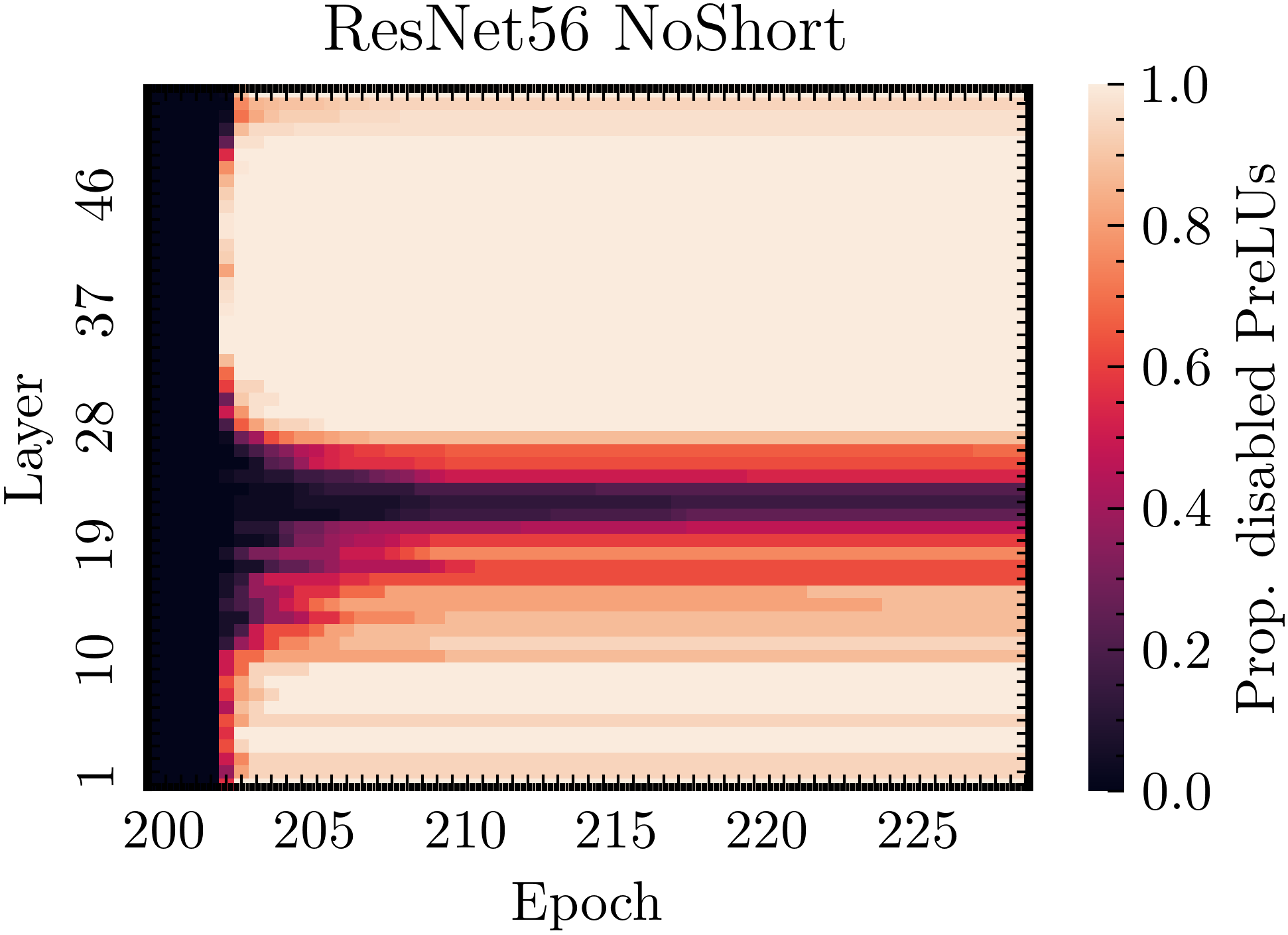
Figure 4: Proportion of inactive PReLUs when partially linearizing a ResNet56 NoShort / Short with $\omega=0.003$.

4.1.2 Nonlinear advantage is stronger in early training

In a second step, we want to break down how linearizing a network at different stages of training affects its performance. For this, we train a ResNet56 Short on datasets of varying difficulty since previous results indicate that we can only measure it on harder datasets. At different stages of the training, we activate our regularizer with a fixed regularization weight, resume training and measure the final performance of the network after a given number of epochs. As regularizing the network at different stages of training with the same regularization weight can result in massive differences in the amount of inactive PReLUs, we slightly modified our regularizer to stop when a goal percentage ($80\pm 1\%$, an amount high enough to impact performance) of inactive PReLUs over all layers is reached. In order not to overshoot our goal percentage, we lower the regularization weight when close to our target. We carefully tune the regularization weight in order to avoid undershooting the target percentage. We see in Figure 3 that networks regularized later in training are significantly more performant than networks partially linearized earlier in training. The biggest differences are visible in the first 15 epochs of training and the effect is particularly pronounced for the harder datasets, indicating a correlation between effect strength and the hardness of the task at hand. In the Appendix in Figure 24 we have shown that for a transformer architecture training on a machine translation task, the test perplexity of networks is higher for networks partially linearized early as opposed to later epochs. The biggest difference occurs within the first 20 epochs of training.

4.2 Performance and Structure of Partially Linearized Networks

Having established in the previous sections that the performance of a network linearized after training cannot simply be recovered by training with a similar amount of nonlinear units from scratch, we now want to understand better how shallow we can make a trained network until performance collapses and where the remaining nonlinearities are located in the network.

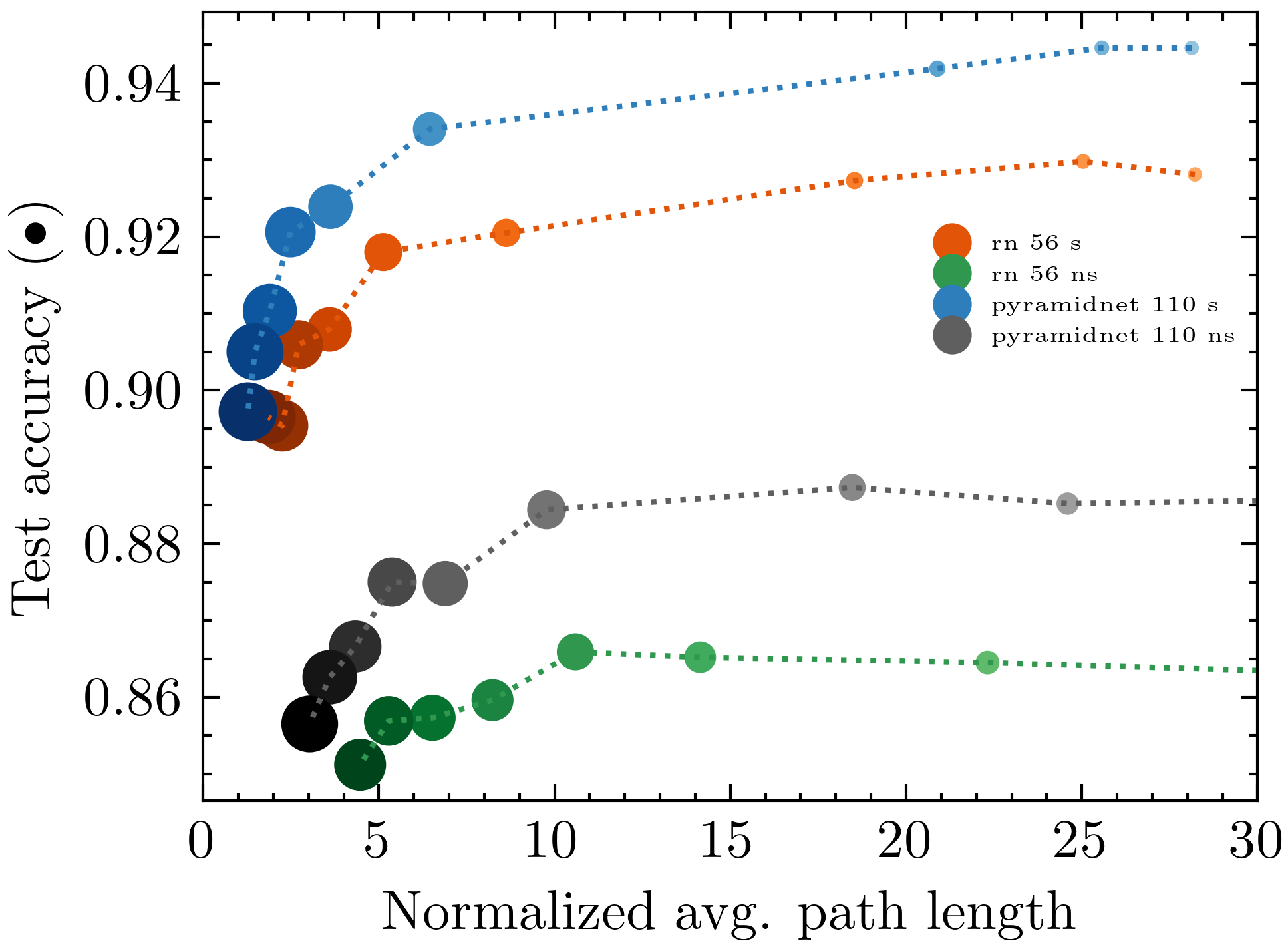
Figure 5: NAPL and test accuracy for different partially linearized network architectures with $\omega\in[0.0005,0.005]$.

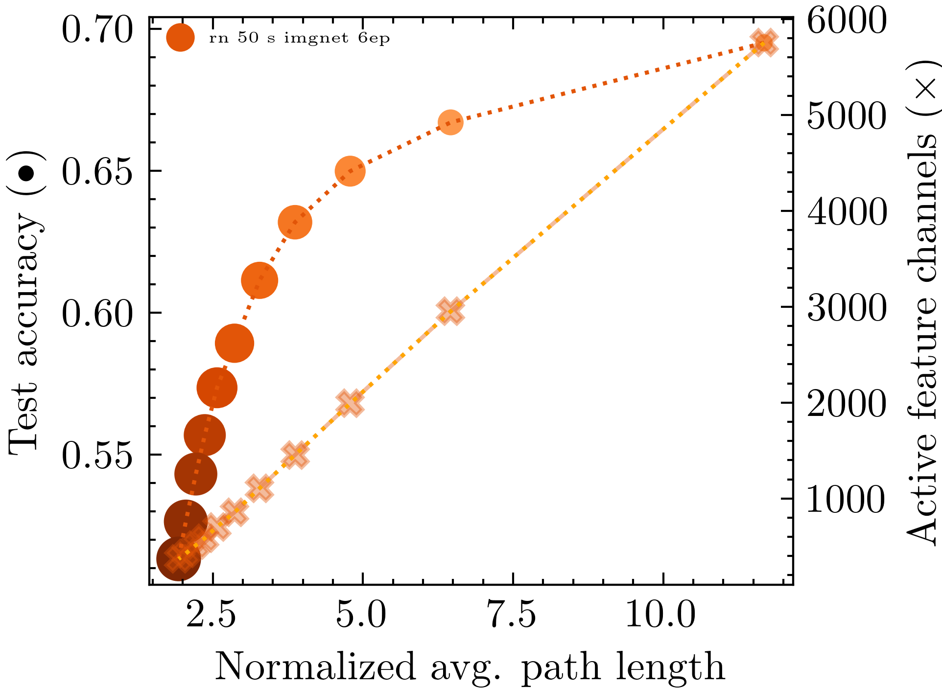
Figure 6: NAPL, accuracy and active features channels for a partially linearized ResNet50 pre-trained on Imagenet with $\omega\in[0.0005,0.0025]$.

We observe the temporal evolution of the linearization process for two different network architectures in Figure 4. When evaluating the proportion of inactive PReLUs per layer, we note that every architecture presents a distinct pattern: for the ResNet56 NoShort, we see that the remaining nonlinearity is concentrated in a connected block, whereas for the ResNet56 Short, the remaining active PReLUs are distributed more evenly over the layers. Interestingly, the connected block of remaining nonlinearity in the ResNet56 NoShort is located in the middle of the network and not on either end, excluding simple vanishing/exploding gradients at initialization effects as a cause. The fact that for the ResNet56 NoShort, many layers are fully linearized without explicit incentive to do so might indicate that such network architectures might not use their full expressive potential. The stripe-like structure of remaining nonlinearities in the ResNet56 Short corresponds to the placement of the residual connections and indicates that these might help in utilizing the full depth of the network. We found the qualitative behavior for both architectures to be consistent on the CIFAR-100 dataset (ref. Appendix), albeit the exact location of the connected nonlinear layer block changes. We conclude that despite regularizing every nonlinear unit equally, distinct patterns form in the remaining nonlinearities in the network that depend on network architecture.

Second, we want to demonstrate the effects of partial linearization on generalization performance for different architectures and datasets. We plotted the performance of partially linearized networks for different choices of $\omega$ on Cifar10 in Figure 6 (ref. Appendix Figure 19 for Cifar100). Darker colors represent a higher regularization weight and the disk sizes represents the global proportion of inactive PReLUs. We can see that for all networks, the top-1 test performance remains high even for a comparably small NAPL values until it collapses. We also see that depending on network architecture, for a similar NAPL value, different networks architectures present a distinct percentage of inactive PReLUs, further supporting our claim of a network-dependent structure being extracted by linearization. A similar plot showing explicitly the proportion of active PReLU units instead of NAPL can be found in the Appendix in Figure 17 (resp. 17 for Cifar100) and shows qualitatively the same behavior. We further verified our claims for a ResNet50 on the ImageNet dataset in Figure 6; note that this network contains a non-ReLU activation layer (maximum pooling) that we included in our calculations by increasing all to the NAPL values by one.

4.3 Analyzing the Shape of the ”Core Network”

In this section, we investigate whether we can find some regularities in the shape of the resulting network if we partially linearize networks of different initial shape.

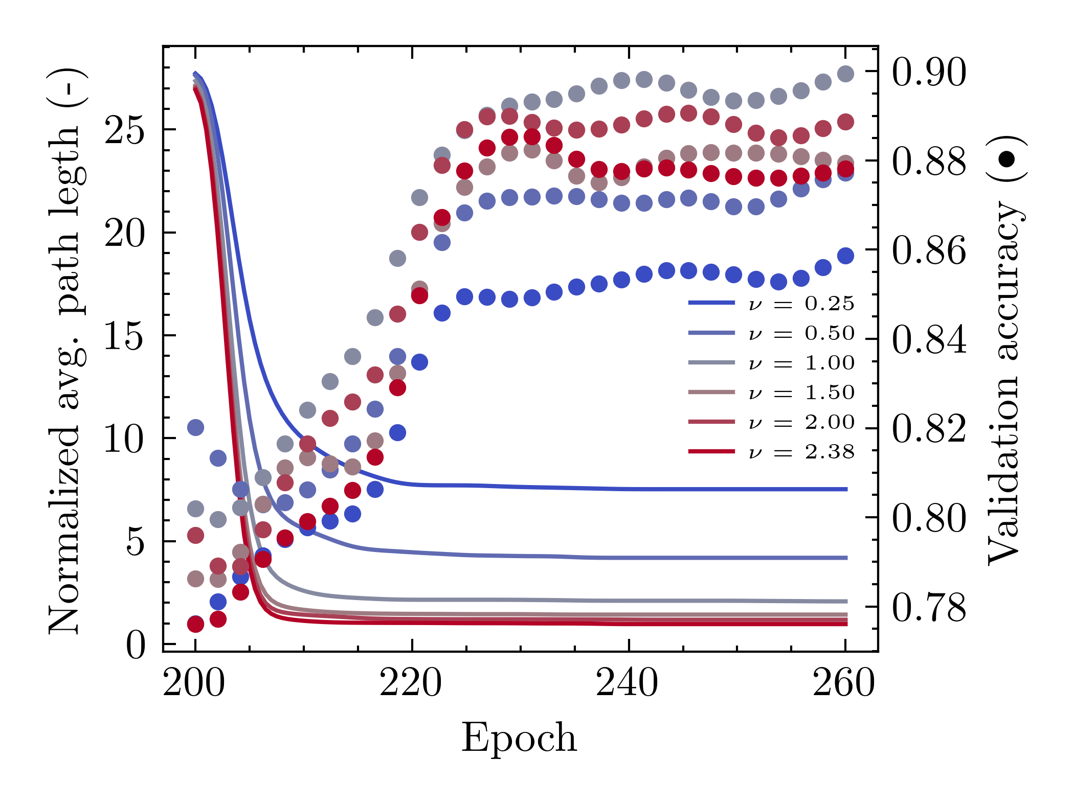
Figure 7: Validation accuracy and average path length during linearization of ResNets56 of different width for $\omega=0.003$.

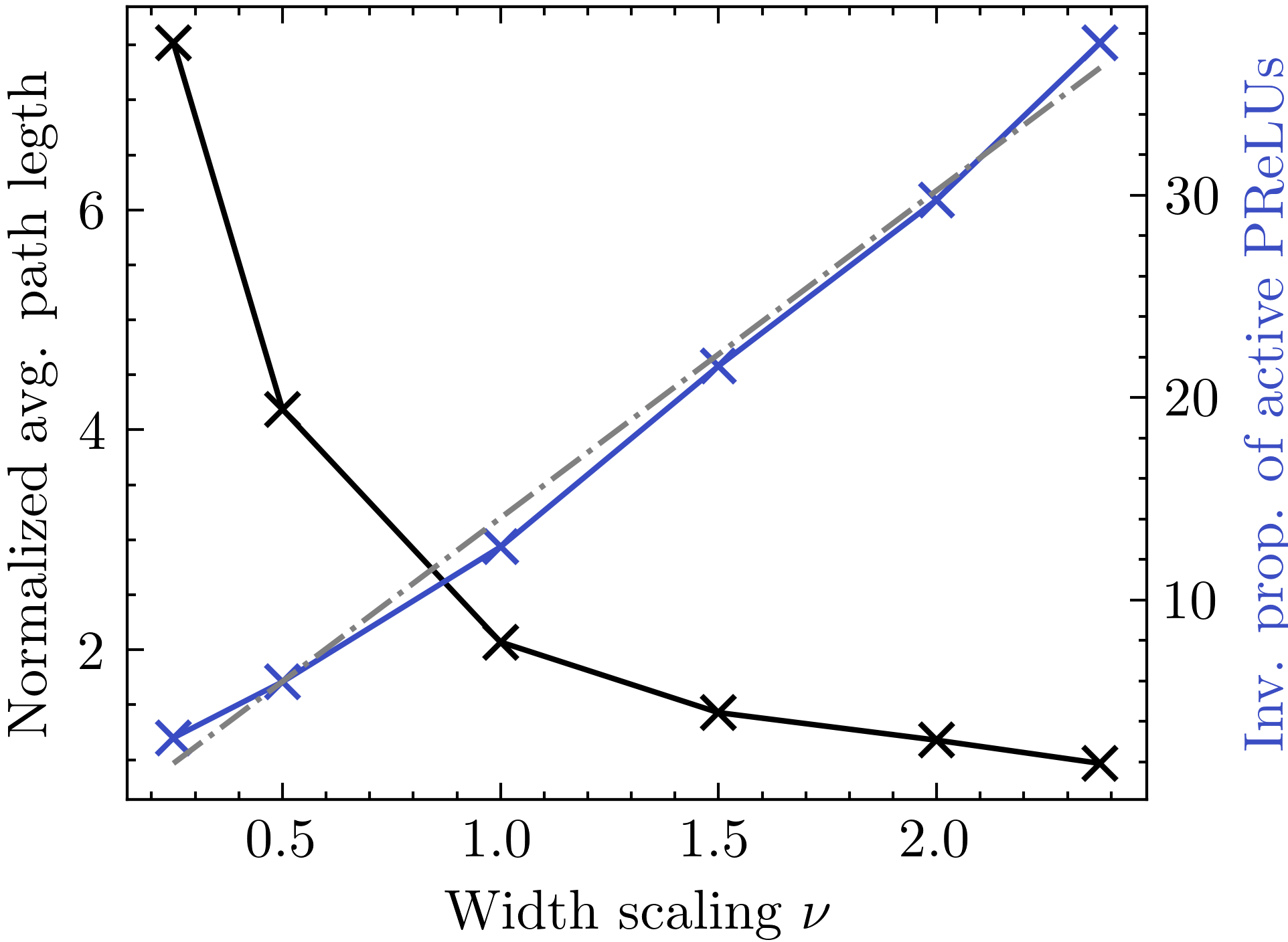
Figure 8: Inverse proportion of active PReLUs and NAPL for ResNet56 Short of different width after linearization for $\omega=0.003$. A linear fit to the blue curve is drawn in grey.

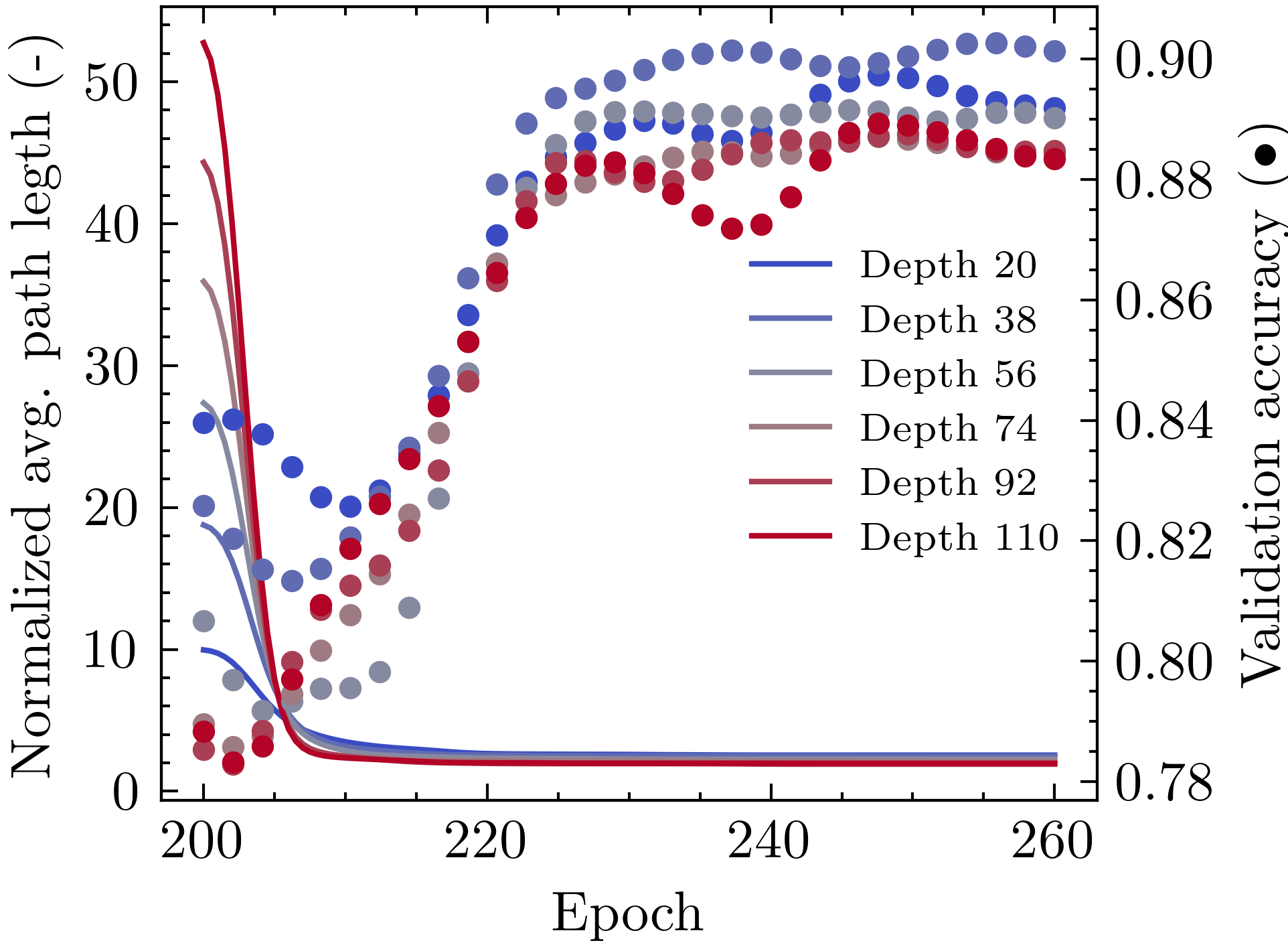
Figure 9: Validation accuracy and average path length during linearization of ResNets of different depth for $\omega=0.003$.

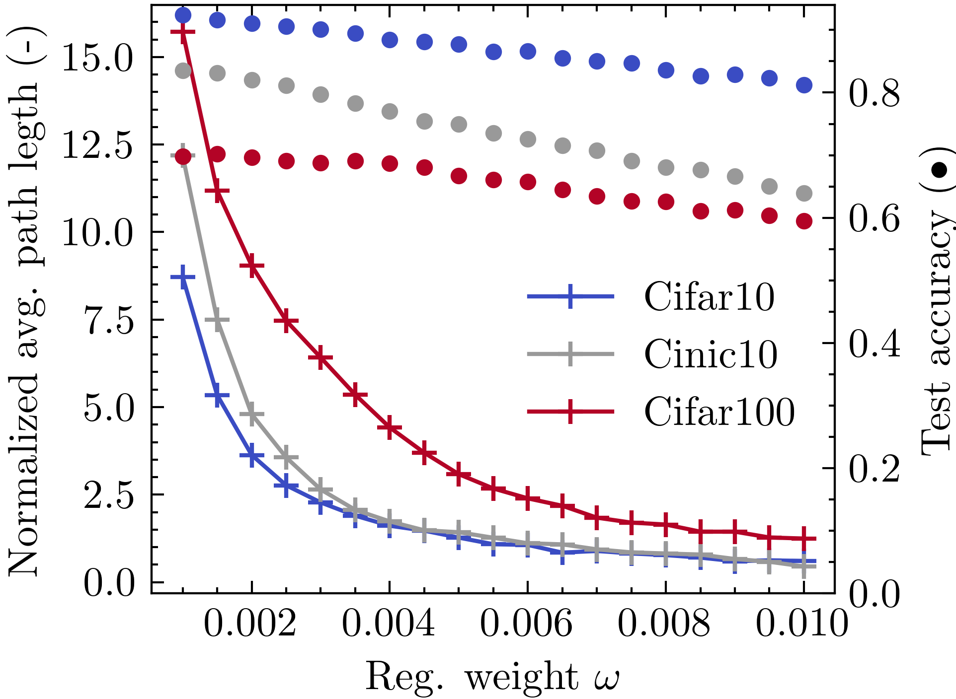
Figure 10: Test accuracy and average path length after linearization of ResNet56 for different regularization weight choices $\omega$ on the Cifar10, CINIC-10 and CIFAR-100 dataset.

4.3.1 ENW Converges Approx. Independently of Initial Width

We now want to analyze the effect of network width on the shape of the resulting partially linearized network. We therefore apply our linearization technique to different versions of ResNet56 Short scaled in width by a factor of $\nu\in\{0.25,0.5,1,1.5,2,2.38\}$ and measure the NAPL and performance of the resulting networks. In Figure 8, we see that wider networks seem to have better performance but lower NAPL. The relationship between the number of filters in a layer and the average path length seems reciprocal: this would imply that the average number of active neurons per layer remains approximately equal. To confirm this, in Figure 8 we plotted the inverse proportion of active PReLUs after post-training linearization for all networks. We can see a linear relationship, confirming that the average amount of active neurons per layer remains roughly constant - independently of the initial width chosen.

4.3.2 NAPL Converges Approx. Independently of Initial Depth

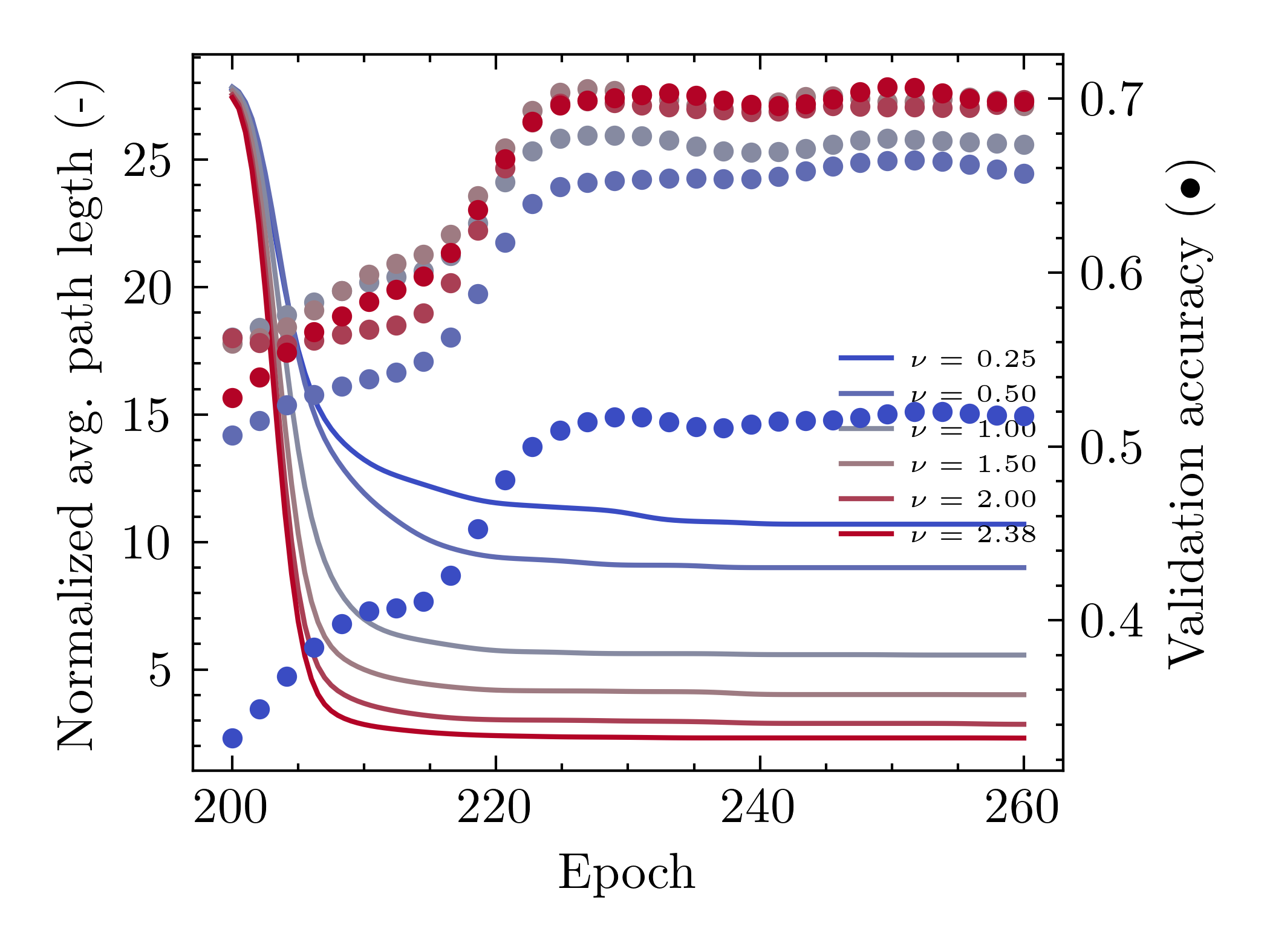
Figure 21: Validation accuracy and NAPL during linearization of ResNets56 of different width for $\omega=0.003$ on CIFAR-100.

We saw that independently of the network width chosen, there was a similar amount of neurons per layer that remained active. We now want to establish if we can make a similar statement with regard to network depth. Therefore, we repeated the experiment of the last section for networks of different depth. In Figure 10, we see that independently of the initial network chosen, the resulting network’s NAPL converges to a similar value while having comparable training performances. Shallower networks seemingly converge to a marginally higher NAPL but this is merely an artifact of how we scaled ResNet blocks and is not observable on a simple convolutional network with constant width (ref. Appendix Figure 24). The results hint the existence of a core nonlinear structure that forms during training that is necessary to learn a given task that is approximately constant in depth and width, regardless of the initial network with chosen. Similar experiments on depth and width on CIFAR-100 in Figure 21 in the Appendix show qualitatively the same behaviour but with different NAPL values.

Note that our method yields better performances than (Dror et al., 2021) for a lower effective depth. The authors obtain a performance of 90.29% / 67.04% for a ResNet56 reduced to 10 layers (that would correspond to a NAPL close to 5) on Cifar10 / Cifar100. We obtained 90.59% / 67.64% for a ResNet56 with NAPL 2.7 / 3.1.

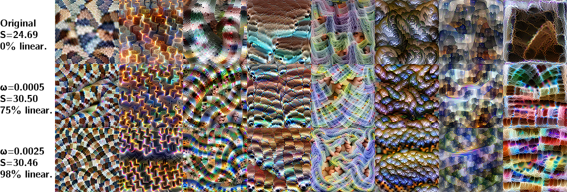
Figure 11: Visualization of the same feature channel per column for a ResNet50 trained on ImageNet across different degrees of partial linearization. The value of $S$ indicates the average image sharpness, measured by the average image gradient magnitude.

4.3.3 NAPL Depends on Task Difficulty

To understand how the difficulty of the task to learn affects the shape of the resulting partially linearized networks, we regularized many instances of ResNet56 Short for different choices of $\omega$ on CIFAR-10, CINIC-10 and CIFAR-100. Looking at Figure 10, we first note that by increasing the regularization weight, the NAPL of the resulting network is decreased as expected, but this effect seems to saturate exponentially while the test accuracy is only reduced linearly in $\omega$. This seems to imply that there is a minimum NAPL necessary to learn a given task. We also see that the NAPL measured is consistently higher for harder datasets (datasets where the networks reach a low top-1 accuracy), except for very high regularization values where the CINIC-10 and CIFAR-10 curves converge. We conclude that our method is able to extract a network with minimal nonlinearity able to learn a given task.

4.4 Impact on Feature Visualizations

Finally, we visualized some feature channels from ResNet50 Short trained on ImageNet and partly linearized to different degrees ($\omega\in[0,0.0005,0.0025]$) with the Lucent (Kiat, 2021) library; the performance and amount of remaining active PReLU units in these networks is shown in Figure 6. We only consider feature channels that are still active in all three networks and chose one of the deeper layers for visualization in Figure 11. We see that in most cases, we can recognize a given feature over the different networks and the image seems subjectively sharper for the partially linearized networks. To confirm this, we measured the magnitude of the image gradient, averaged over all 1721 feature channels remaining in all three network and rgb-channels. This sharpness measure (indicated as $S$) is indeed significantly higher for the linearized networks, but we cannot discern a further increase for the network with higher degree of linearization.

5 Summary of Contributions and Discussion

In our work, we observe that linearized networks extracted after training outperform networks with the same amount of nonlinear units trained from scratch in experiments on convolutional and transformer architectures trained on computer vision and machine translation tasks. This is a highly surprising observation, as the final network architecture and thus it’s expressivity are the same, but still, worse minima are found when training shallow architectures from scratch as opposed to training a deeper architecture and making it shallower afterwards. This is, to our best knowledge, the first time such an effect is described in literature. Complementary findings in recent literature describe a similar effect of finding a simpler ”core structure” contained in the network in early training: for fully linearizing the network with regard to its weights (time/data-dependent NTK) (Fort et al., 2020) and for drawing ”lottery tickets” (You et al., 2020). By reducing nonlinearity at channel-level, our method is able to extract networks containing significantly less nonlinear units while maintaining a similar performance, compared to previous attempts (Dror et al., 2021). We conclude that theoretical results analyzing very shallow networks e.g. (Safran et al., 2022) might have higher significance on networks used in practice than previously thought and that network depth mostly benefits the training process in early stages, as most of their nonlinear expressive power or depth is not utilized after training.

Since our method prunes nonlinearity at a channel-level as opposed to network weights, it is easier to relate the reduction in complexity to function space in terms of effective width and depth. In order to sensibly characterize the depth of a network with many linearized channels, we introduce the average path length of a network, a measure that counts the average number of nonlinear units encountered over all paths in the computation graph of the network. Linearizing networks to different degrees then allows us to characterize the minimum effective width and depth needed in order to solve a given problem. In experiments on multiple computer vision datasets, we found that these values are roughly constant for a given problem and fixed regularization weight, independently of the initial network chosen and that that the effective depth of a network grows with problem complexity. Further, we found that the essential nonlinear units in a network are distributed rather uniformly over the layers for residual networks as opposed to plain feedforward networks where they seem form clusters. This indicates that in deep networks without residual connections, there could be large connected blocks of layers that contribute very little to the learned function’s nonlinear complexity.

Finally, since our method drastically reduces the amount of nonlinear feature channels in a network, we envision it can be useful for researchers trying to explain a network’s behavior through visual inspection of its features. Our method not only reduces the number of nonlinear feature channels but also measurably increases the sharpness of gradient-based feature visualizations.

6 Acknowledgments

The authors acknowledge funding from the Emergent AI Center funded by the Carl-Zeiss-Stiftung. The authors would like to thank Daniel Franzen and Michael Wand for their helpful discussions.

Appendix A Details About Histogram Computation

Figure 12: Computing the histogram of path lengths through dynamic programming for a non-residual (left) and a residual (right) network. Red circles designate nodes with an active PReLU activation, blue edges designate residual connections.

A.1 Normalizing the Histogram

Veit et al. (2016) also study the distribution of path lengths in neural networks. To model the path distribution in a residual network, the authors simply use a binomial distribution, giving the main and residual branch of a residual block equal weight. Since the authors use a binomial distribution to model path length, the average path length of a ResNet of depth $d$ before linearization is $d/2$ in their model. Figure 13 (left) makes it clear that in our (non-normalized) model as described above, the average path length would be much closer to $d$ since the main path contribution is exponentially bigger than the residual path contribution and thus vanishes in depth.

In order to obtain an equal contribution from the main branch and the residual branch of residual block, we can modify our model to normalize the histograms before adding them together as shown in Figure 13 (right). Since we explicitly modeled the length of residual connections (how many layers are skipped), the path length of a ResNet before linearization depends on ResBlock size in our model. For a standard ResNet using BasicBlock (ResBlock size 2), we found the initial NAPL to be close to $d/2$, making our normalized average path length model similar to the one from Veit et al. (2016).

Figure 13: Computing the unnormalized (left) and normalized (right) histogram of a residual network where all PReLUs are active. Without normalization, the residual contribution vanishes.

Appendix B Complementary Experiments

B.1 Plots for APL Instead of NAPL

In this section, we repeat the experiments of Figure 6, 10 and 8 showing APL instead of NAPL. In Figure 19, 15 and 15, we see fundamentally no differ ence in the results except for all unnormalized path length values being consistently higher than the normalized ones.

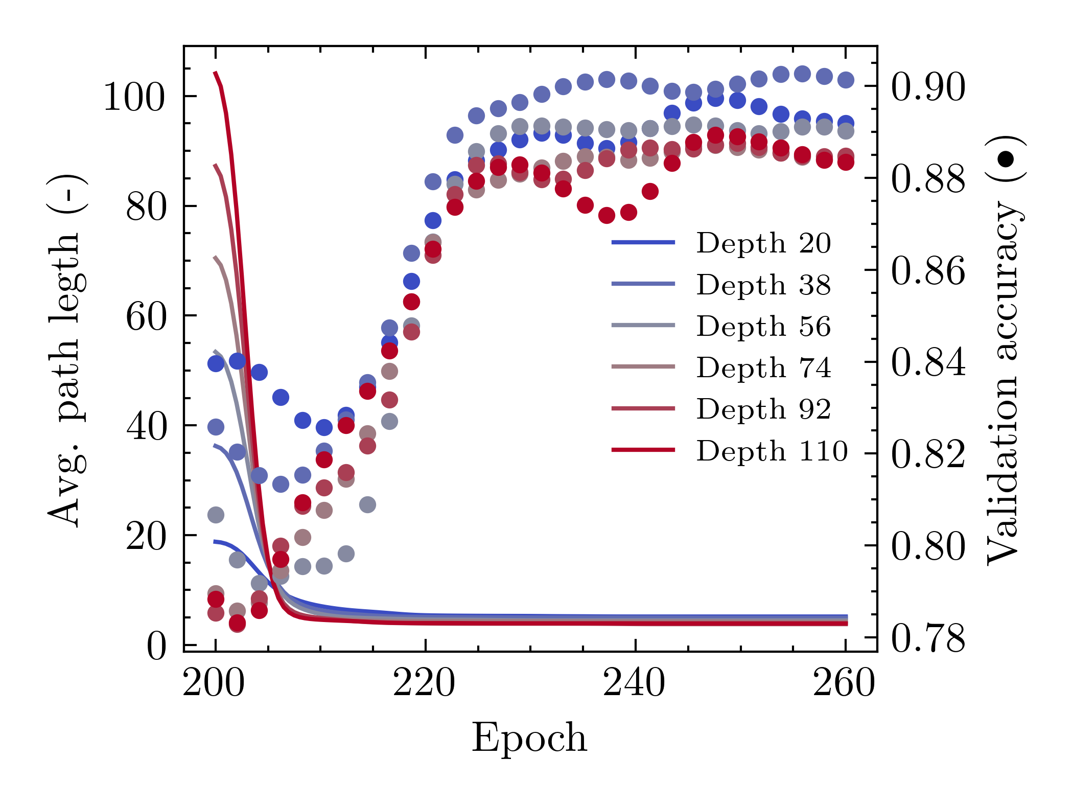
Figure 14: Validation accuracy and unnormalized average path length during linearization of ResNets of different depth for $\omega=0.003$.

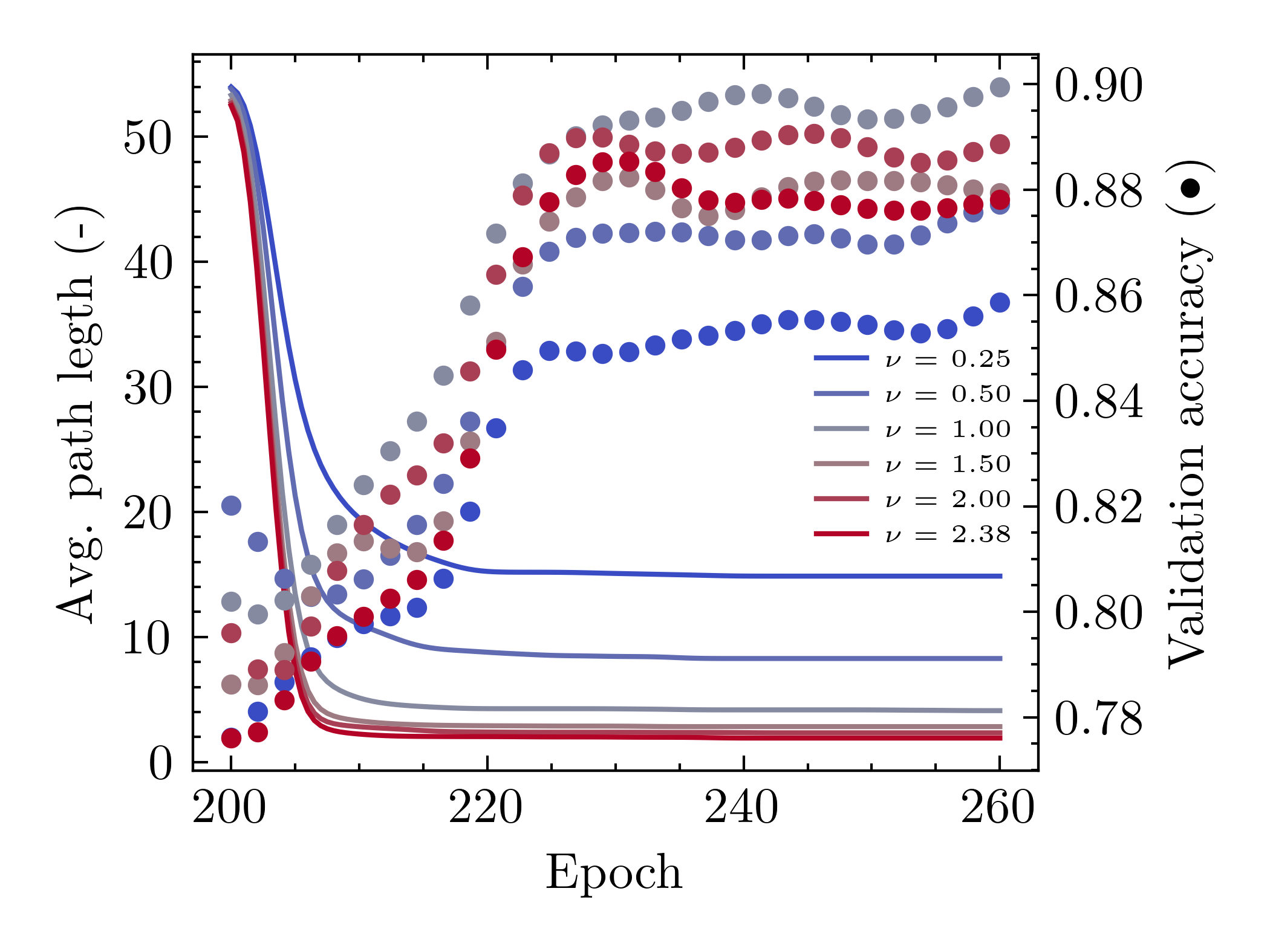
Figure 15: Validation accuracy and unnormalized average path length during linearization of ResNets of different width for $\omega=0.003$.

B.2 Plots for Active PReLU Percentage Instead of NAPL

In Figure 17 (resp. 17 for Cifar-100) show the results of Figure 6 (resp. 19) but plotting the global percentage of active PReLU units instead of NAPL on the x-axis. We see that qualitatively, we obtain a very similar result. This serves as sanity-check our our (N)APL measure, showing that the measurements made qualitatively correspond to the ones made with a much simpler measure.

Figure 16: Proportion of active PReLU units and test accuracy for different network architectures with regularization weight $\omega\in[0.0005,0.005]$.

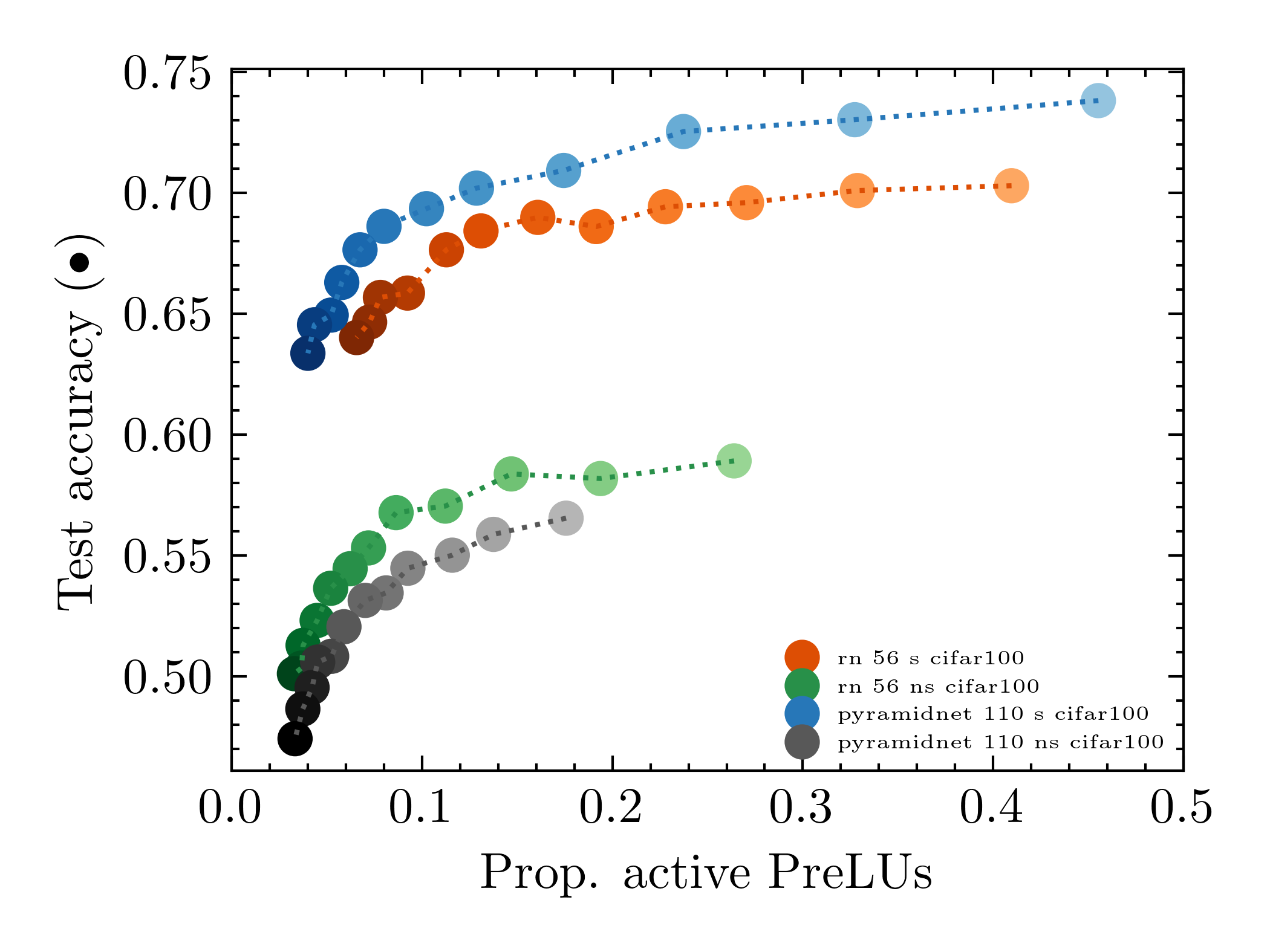
Figure 17: Proportion of active PReLU units and test performance (left) for different network architectures with regularization weight $\omega\in[0.0015,0.007]$ on CIFAR-100..

B.3 Experiments on Cifar100

In Figure 22, 19, 21 and 21 we repeated the experiments of Figure 4, 6, 10, 8 on CIFAR-100 and see qualitatively the same behaviour although all measured NAPL value are consistently higher than on CIFAR-10.

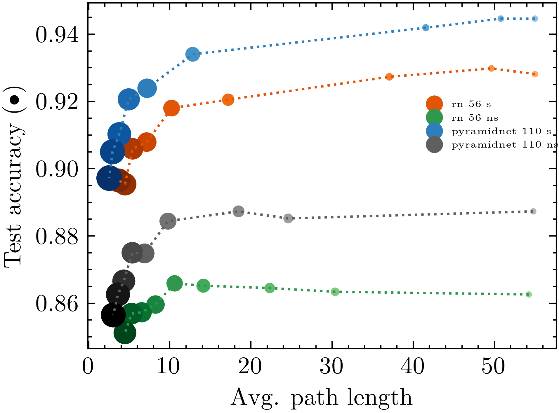
Figure 18: Unnormalized average path length and test accuracy for different network architectures with regularization weight $\omega\in[0.0005,0.005]$.

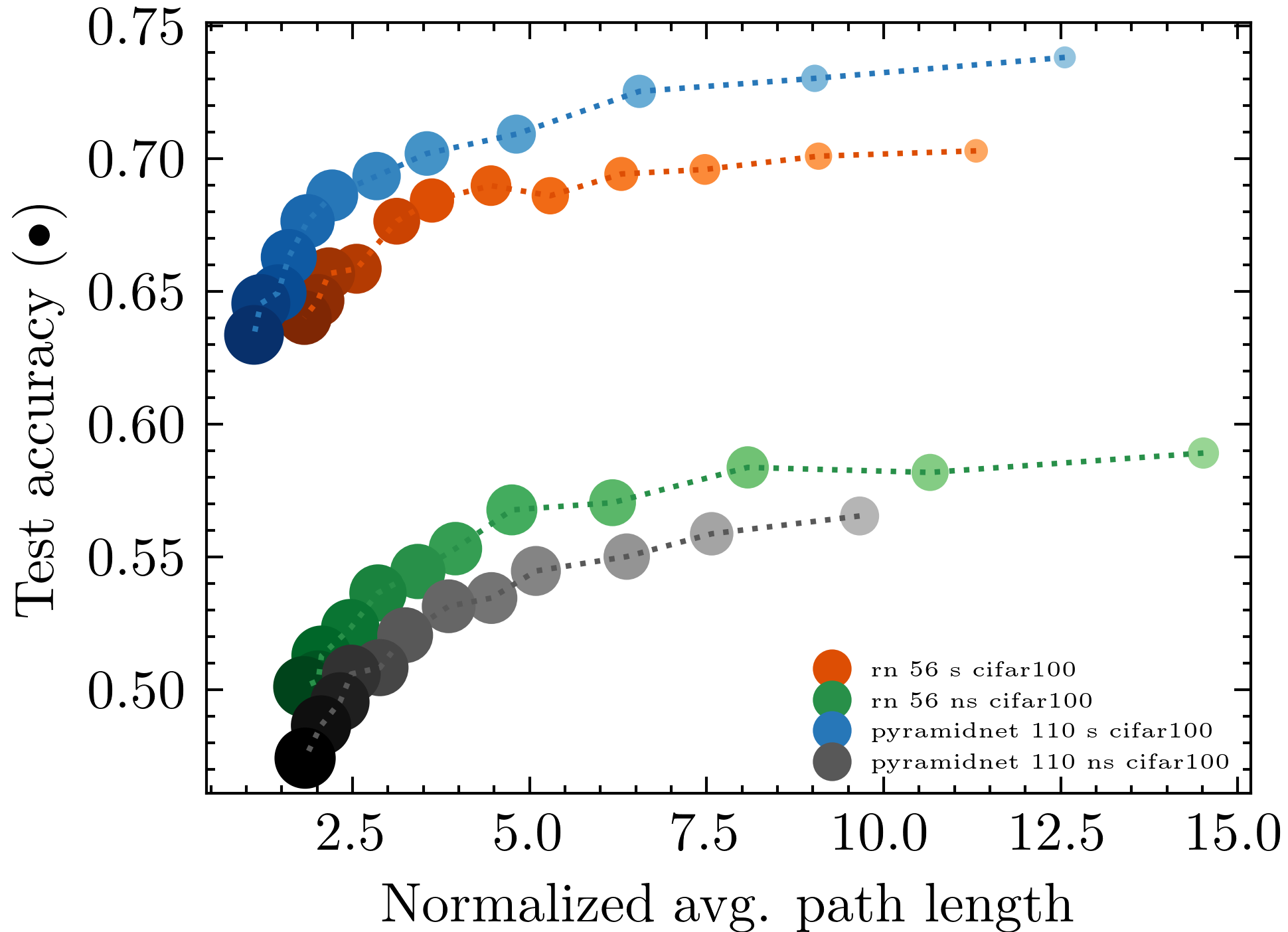
Figure 19: Normalized average path length and test performance (left) for different network architectures with regularization weight $\omega\in[0.0015,0.007]$ on CIFAR-100.

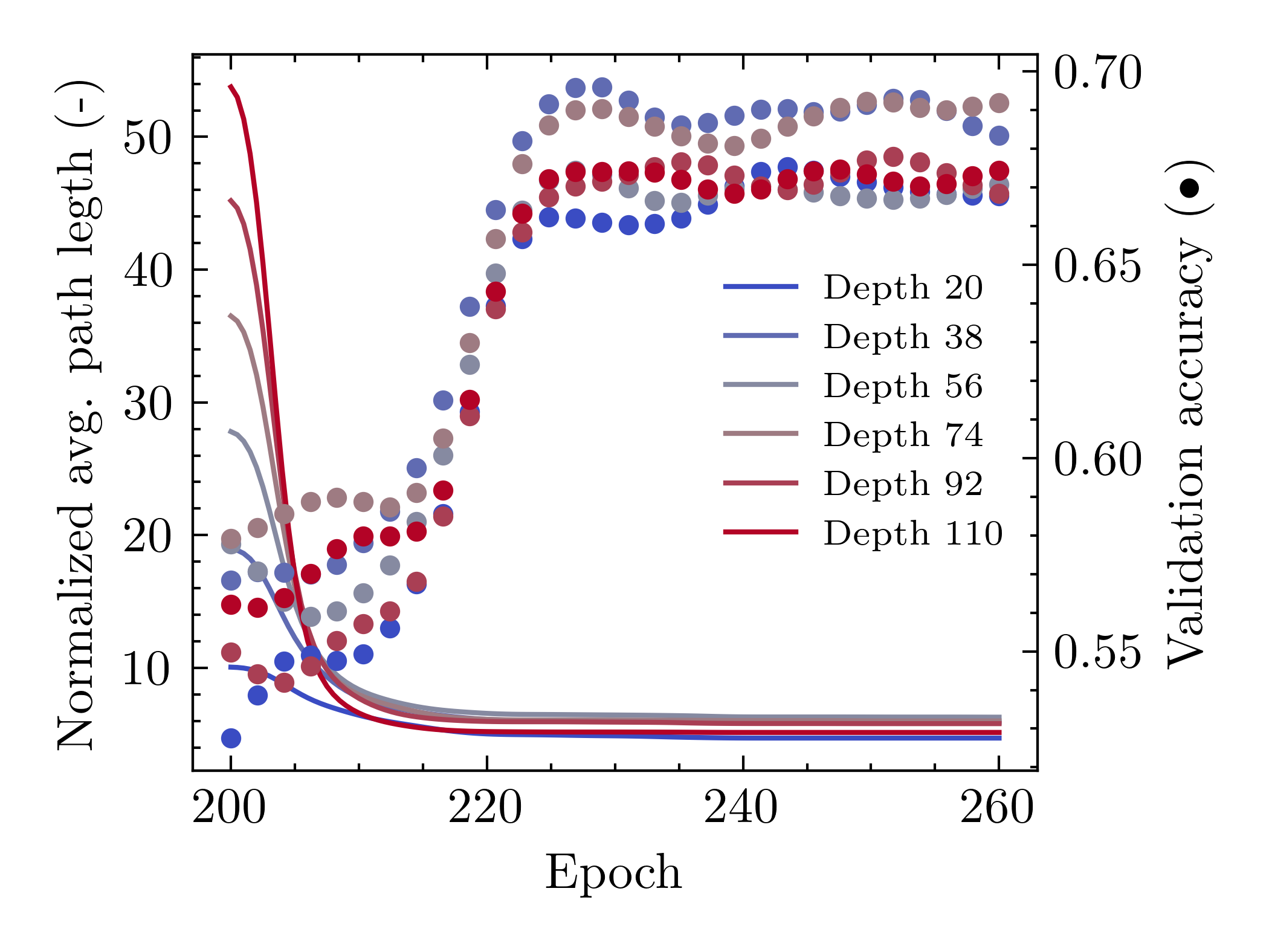
Figure 20: Validation accuracy and NAPL during linearization of ResNets of different depth for $\omega=0.003$ on CIFAR-100.

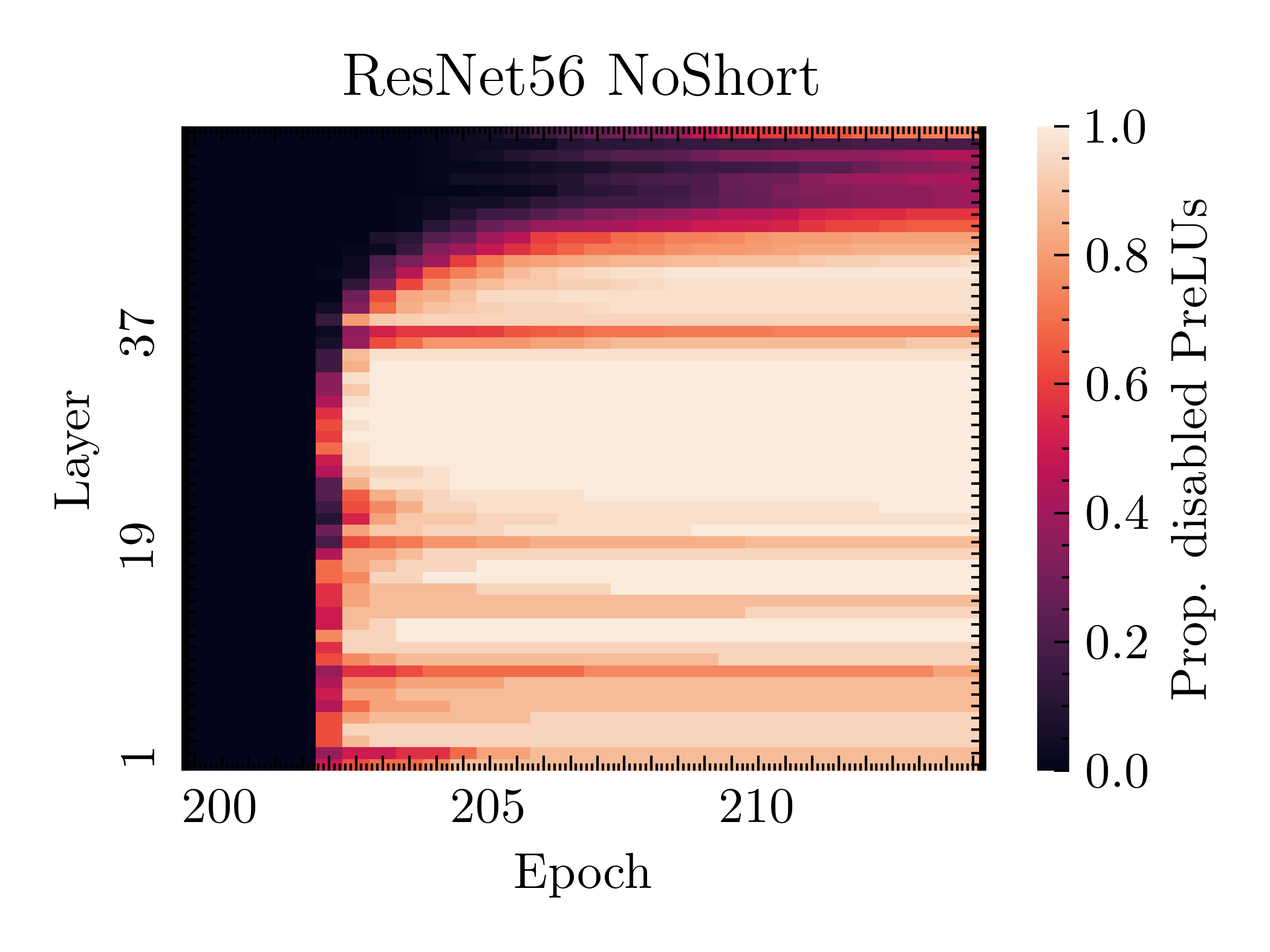
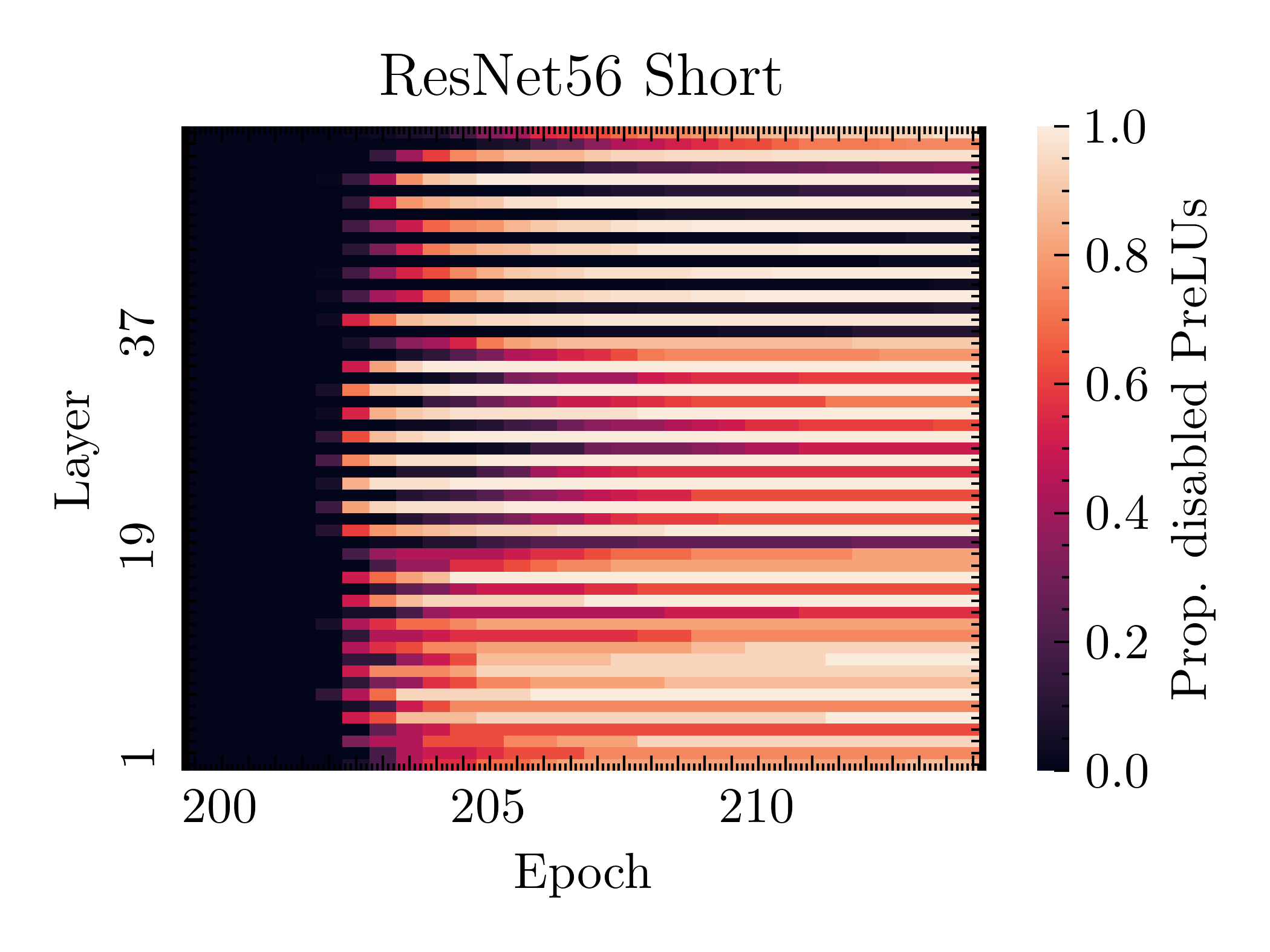
Figure 22: Proportion of inactive PReLUs when linearizing a ResNet56 NoShort / Short with $\omega=0.003$ on CIFAR-100.

B.4 APL of Networks with Constant Width

In Figure 10, we analyzed the average path length of ResNets of different size after applying our post-training linearization procedure. In Figure 10 all networks seem to converge approximately to the same APL independently of network depth, but shallower networks seem to yield a slightly higher APL. We wanted to further investigate this pattern.

In Figure 24, we repeated the same experiment with a simplistic Toy-Net having constant width and no striding after the first layer and see the pattern dissapear completely. We conclude that the observed pattern is an artifact of scaling ResBlocks of different width and striding operations in the network.

B.5 Nonlinear Advantage on Transformer Architectures

In Figure 24, we repeated the experiment of Figure 3 for a transformer network training on the Multi30k german-english translation task. We decided to linearize $100\%$ of all PReLU activations, as transformer architectures contain more nonlinearities than just ReLU units and we need to remove enough nonlinearity in the network in order to significantly impact performance. We see the result of the main section confirmed: networks linearized at a later stage of training outperform networks linearized earlier on.

Appendix C Architecture and Training Details

C.1 Architecture Details

As described in the main paper, we used a ResNet architecture with BasicBlock v2 and BasicBlockPyramid with and without residual connections for the CIFAR-10 / CINIC-10 / CIFAR-100 runs. We used shortcut option ”A” (padding) for all networks except in Section 4.3.1 where option ”B” (1x1 convolutions) is needed to make the network work with different widths. We used the default number of planes $num\_planes=(16,32,64)$ for each BasicBlock, except for Figure 8 where the number of planes is multiplied by a constant $\nu$. For Figure 10, we used $num\_blocks=(i,i,i),~{}i\in\{3,6,9,12,15,18\}$ to scale the number of blocks in the ResNet. PyramidNet 41 resp. 110 uses $num\_blocks=(3,4,6)$ resp. $18,18,18$ and $num\_planes=(32,128)$ resp $num\_planes=(16,100)$ with shortcut option ”A”.

For the ImageNet runs, we used the ResNet50 architecture from the official TorchVision repository.

For Figure 24, we used a simple Conv-BN-ReLU ToyNet with constant width (32 Filters), no striding after the first layer, residual connections of length 1 and a final fully connected layer.

Details of the transformer architecture can be found in Figure 25 (left).

C.2 (Post-)Training Hyperparmeters & Hardware

The experiments in the paper were made on computers running Arch Linux, Python 3.10.5, PyTorch Version 1.11.0+cu102. The GPUs used were NVIDIA GeForce GTX 1080 Ti and NVIDIA GeForce RTX 2080 Ti.

The hyper-parameters in Figure 26 were used to (post-) train on the CIFAR-10, CINIC-10 and CIFAR-100 and usually reach the standard test-accuracy of approximately $92.7$ for a ResNet56 on CIFAR-10. As for the ImageNet runs, we used a pre-trained model from the torchvision model-zoo. For post-training, the hyper-parameters in Figure 27 were used. For the CINIC-10 post-training, we adapted the number of epochs and the multistep scheduler milestones to approximately maintain the same number of batches since the total number of training images is different.

Note: The experiments of Figure 3 and 4 have a shorter post-train phase of 30 epochs instead of 60 epochs (the multistep milestones are 10/20) to save compute, as these experiments do not aim for maximum accuracy.

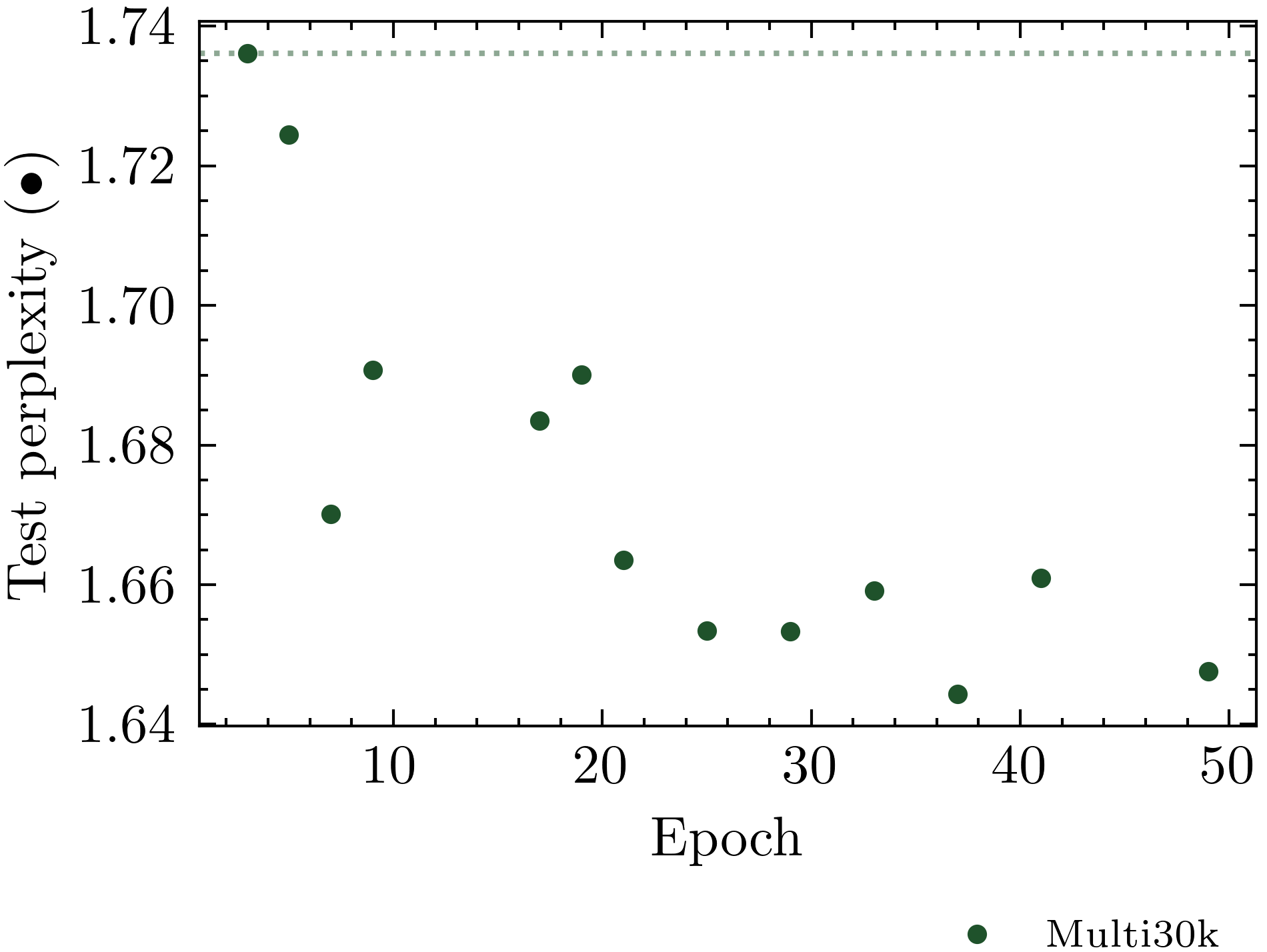
Figure 23: Test perplexity of a transformer network partially linearized at different epochs during training on a translation task. The dotted line indicates the height of the first datapoint for visual reference.

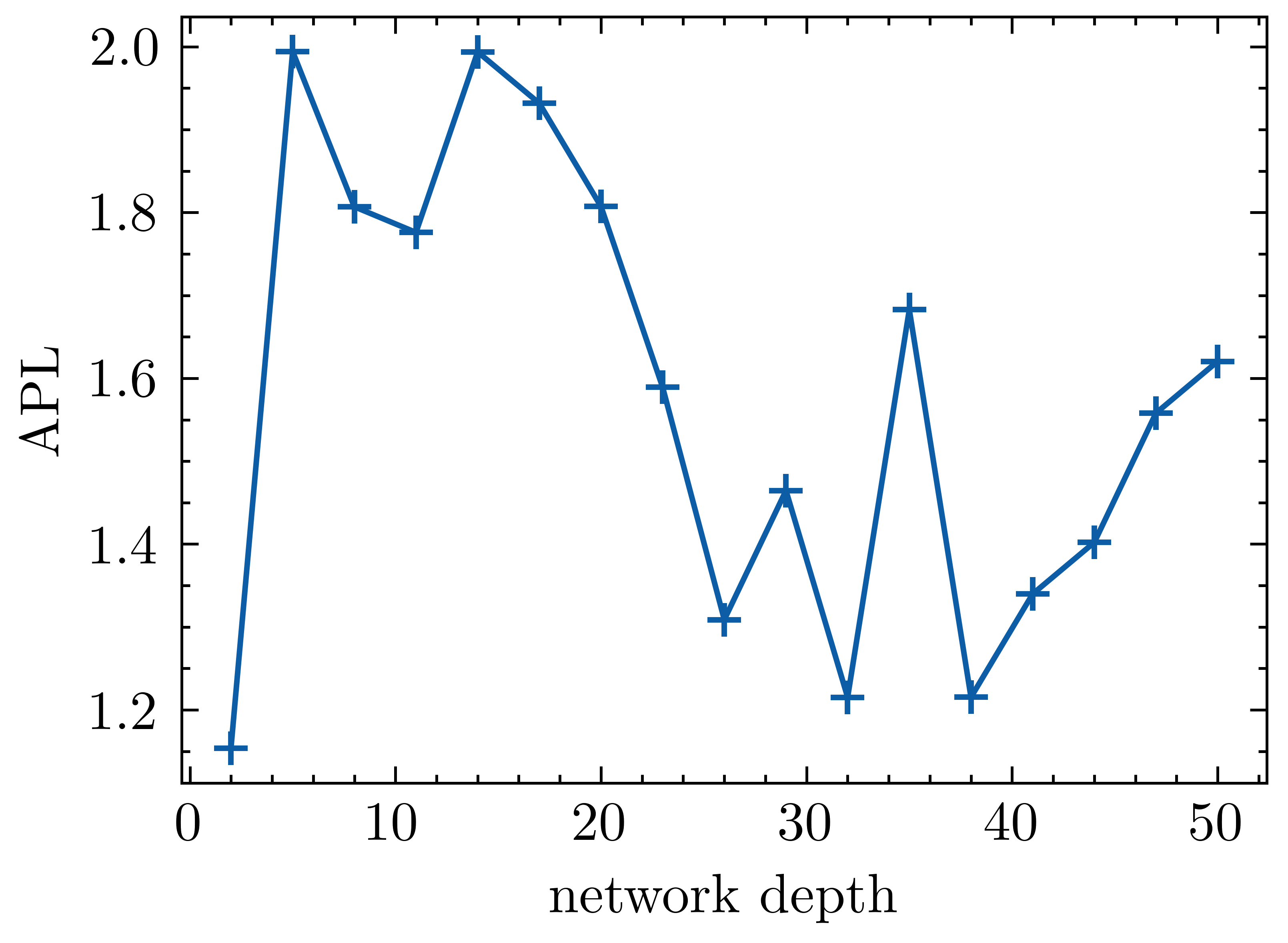
Figure 24: Average path length of Toy-Nets of different depth after post-training linearization for $\omega=0.003$.

Architecture	Transformer
$d_{ff}$	2048
$d_{model}$	512
$h$	8
$N$	6
$p_{dropout}$	0.1

Training	Multi30k
Epochs	200
Scheduler	Warmup+Multistep ($\gamma=0.1$)
Warmup steps	2900
Milestones	160, 180
Learning rate	0.00082
Batch size	30
Gradient accumulation	10 steps
Optimizer	ADAM
$(\beta_{1},\beta_{2})$	(0.9, 0.98)
Weight decay	0
Label Smoothing	0.1

Figure 25: Architecture details and training regime for the NLP task.

Training	CIFAR-10 / CINIC-10 / CIFAR-100
Epochs	200
Scheduler	Multistep ($\gamma=0.1$)
Milestones	100, 150
Learning rate	0.1
Batch size	256
Optimizer	SGD + Momentum
Momentum	0.9
Weight decay	0.0001
Augmentation	Random Flip

Training	TinyImagenet
Epochs	80
Scheduler	Multistep ($\gamma=0.1$)
Milestones	70, 75
Learning rate	0.1
Batch size	128
Optimizer	SGD + Momentum
Momentum	0.9
Weight decay	0.0001
Augmentation	Random Flip

Figure 26: Details of the training regime for CV tasks.

Post-Training	CIFAR-10 / CINIC-10 / CIFAR-100
Epochs	60 (34 for CINIC-10)
Scheduler	Multistep ($\gamma=0.1$)
Milestones	20, 40 (10, 22 for CINIC-10)
Learning rate	0.1
Batch size	256
Optimizer	SGD + Momentum
Momentum	0.9
Weight decay	0.0001
Augmentation	Random Flip

Post-Training	Imagenet
Epochs	6
Scheduler	Multistep ($\gamma=0.1$)
Milestones	2, 4
Learning rate	0.01
Batch size	40
Optimizer	SGD + Momentum
Momentum	0.9
Weight decay	0.0001
Augmentation	Center Crop (224 px.)

Figure 27: Details of the post-training regime.

References

- Ali Mehmeti-Göpel et al. (2021) Ali Mehmeti-Göpel, C. H. X., Hartmann, D., and Wand, M. Ringing relus: Harmonic distortion analysis of nonlinear feedforward networks. In 9th International Conference on Learning Representations, ICLR 2021, Virtual Event, Austria, May 3-7, 2021. OpenReview.net, 2021. URL https://openreview.net/forum?id=TaYhv-q1Xit.
- Allen-Zhu et al. (2019) Allen-Zhu, Z., Li, Y., and Liang, Y. Learning and generalization in overparameterized neural networks, going beyond two layers. In Wallach, H. M., Larochelle, H., Beygelzimer, A., d’Alché-Buc, F., Fox, E. B., and Garnett, R. (eds.), Advances in Neural Information Processing Systems 32: Annual Conference on Neural Information Processing Systems 2019, NeurIPS 2019, December 8-14, 2019, Vancouver, BC, Canada, pp. 6155–6166, 2019. URL https://proceedings.neurips.cc/paper/2019/hash/62dad6e273d32235ae02b7d321578ee8-Abstract.html.
- Arora et al. (2019) Arora, S., Li, Z., and Lyu, K. Theoretical analysis of auto rate-tuning by batch normalization. In 7th International Conference on Learning Representations, ICLR 2019, New Orleans, LA, USA, May 6-9, 2019. OpenReview.net, 2019. URL https://openreview.net/forum?id=rkxQ-nA9FX.
- Balduzzi et al. (2017) Balduzzi, D., Frean, M., Leary, L., Lewis, J. P., Ma, K. W., and McWilliams, B. The shattered gradients problem: If resnets are the answer, then what is the question? In Precup, D. and Teh, Y. W. (eds.), Proceedings of the 34th International Conference on Machine Learning, ICML 2017, Sydney, NSW, Australia, 6-11 August 2017, volume 70 of Proceedings of Machine Learning Research, pp. 342–350. PMLR, 2017. URL http://proceedings.mlr.press/v70/balduzzi17b.html.
- Bartlett et al. (2019) Bartlett, P. L., Harvey, N., Liaw, C., and Mehrabian, A. Nearly-tight vc-dimension and pseudodimension bounds for piecewise linear neural networks. J. Mach. Learn. Res., 20:63:1–63:17, 2019. URL http://jmlr.org/papers/v20/17-612.html.
- Belkin et al. (2019) Belkin, M., Hsu, D., Ma, S., and Mandal, S. Reconciling modern machine-learning practice and the classical bias–variance trade-off. Proceedings of the National Academy of Sciences, 116(32):15849–15854, 2019.
- Cybenko (1989) Cybenko, G. Approximation by superpositions of a sigmoidal function. Math. Control. Signals Syst., 2(4):303–314, 1989. doi: 10.1007/BF02551274. URL https://doi.org/10.1007/BF02551274.
- Darlow et al. (2018) Darlow, L. N., Crowley, E. J., Antoniou, A., and Storkey, A. J. CINIC-10 is not imagenet or CIFAR-10. CoRR, abs/1810.03505, 2018. URL http://arxiv.org/abs/1810.03505.
- Deng et al. (2009) Deng, J., Dong, W., Socher, R., Li, L., Li, K., and Fei-Fei, L. Imagenet: A large-scale hierarchical image database. In 2009 IEEE Computer Society Conference on Computer Vision and Pattern Recognition (CVPR 2009), 20-25 June 2009, Miami, Florida, USA, pp. 248–255. IEEE Computer Society, 2009. doi: 10.1109/CVPR.2009.5206848. URL https://doi.org/10.1109/CVPR.2009.5206848.
- Dror et al. (2021) Dror, A. B., Zehngut, N., Raviv, A., Artyomov, E., Vitek, R., and Jevnisek, R. J. Layer folding: Neural network depth reduction using activation linearization. CoRR, abs/2106.09309, 2021. URL https://arxiv.org/abs/2106.09309.
- Elliott et al. (2016) Elliott, D., Frank, S., Sima’an, K., and Specia, L. Multi30k: Multilingual english-german image descriptions. In Proceedings of the 5th Workshop on Vision and Language, hosted by the 54th Annual Meeting of the Association for Computational Linguistics, VL@ACL 2016, August 12, Berlin, Germany. The Association for Computer Linguistics, 2016. doi: 10.18653/v1/w16-3210. URL https://doi.org/10.18653/v1/w16-3210.
- Fort et al. (2020) Fort, S., Dziugaite, G. K., Paul, M., Kharaghani, S., Roy, D. M., and Ganguli, S. Deep learning versus kernel learning: an empirical study of loss landscape geometry and the time evolution of the neural tangent kernel. In Larochelle, H., Ranzato, M., Hadsell, R., Balcan, M., and Lin, H. (eds.), Advances in Neural Information Processing Systems 33: Annual Conference on Neural Information Processing Systems 2020, NeurIPS 2020, December 6-12, 2020, virtual, 2020. URL https://proceedings.neurips.cc/paper/2020/hash/405075699f065e43581f27d67bb68478-Abstract.html.
- Frankle & Carbin (2019) Frankle, J. and Carbin, M. The lottery ticket hypothesis: Finding sparse, trainable neural networks. In 7th International Conference on Learning Representations, ICLR 2019, New Orleans, LA, USA, May 6-9, 2019. OpenReview.net, 2019. URL https://openreview.net/forum?id=rJl-b3RcF7.
- Gebhart et al. (2021) Gebhart, T., Saxena, U., and Schrater, P. A unified paths perspective for pruning at initialization. CoRR, abs/2101.10552, 2021. URL https://arxiv.org/abs/2101.10552.
- Han et al. (2017) Han, D., Kim, J., and Kim, J. Deep pyramidal residual networks. In 2017 IEEE Conference on Computer Vision and Pattern Recognition, CVPR 2017, Honolulu, HI, USA, July 21-26, 2017, pp. 6307–6315. IEEE Computer Society, 2017. doi: 10.1109/CVPR.2017.668. URL https://doi.org/10.1109/CVPR.2017.668.
- Hanin & Rolnick (2019) Hanin, B. and Rolnick, D. Deep relu networks have surprisingly few activation patterns. In Wallach, H. M., Larochelle, H., Beygelzimer, A., d’Alché-Buc, F., Fox, E. B., and Garnett, R. (eds.), Advances in Neural Information Processing Systems 32: Annual Conference on Neural Information Processing Systems 2019, NeurIPS 2019, December 8-14, 2019, Vancouver, BC, Canada, pp. 359–368, 2019. URL https://proceedings.neurips.cc/paper/2019/hash/9766527f2b5d3e95d4a733fcfb77bd7e-Abstract.html.
- He et al. (2015a) He, K., Zhang, X., Ren, S., and Sun, J. Delving deep into rectifiers: Surpassing human-level performance on imagenet classification. In 2015 IEEE International Conference on Computer Vision, ICCV 2015, Santiago, Chile, December 7-13, 2015, pp. 1026–1034. IEEE Computer Society, 2015a. doi: 10.1109/ICCV.2015.123. URL https://doi.org/10.1109/ICCV.2015.123.
- He et al. (2015b) He, K., Zhang, X., Ren, S., and Sun, J. Delving deep into rectifiers: Surpassing human-level performance on imagenet classification. In 2015 IEEE International Conference on Computer Vision, ICCV 2015, Santiago, Chile, December 7-13, 2015, pp. 1026–1034. IEEE Computer Society, 2015b. doi: 10.1109/ICCV.2015.123. URL https://doi.org/10.1109/ICCV.2015.123.
- He et al. (2016) He, K., Zhang, X., Ren, S., and Sun, J. Identity mappings in deep residual networks. In Leibe, B., Matas, J., Sebe, N., and Welling, M. (eds.), Computer Vision - ECCV 2016 - 14th European Conference, Amsterdam, The Netherlands, October 11-14, 2016, Proceedings, Part IV, volume 9908 of Lecture Notes in Computer Science, pp. 630–645. Springer, 2016. doi: 10.1007/978-3-319-46493-0“˙38.
- Hochreiter (1991) Hochreiter, S. Untersuchungen zu dynamischen neuronalen netzen. Diploma thesis, TU Munich, 1991.
- Ioffe & Szegedy (2015) Ioffe, S. and Szegedy, C. Batch normalization: Accelerating deep network training by reducing internal covariate shift. In Bach, F. R. and Blei, D. M. (eds.), Proceedings of the 32nd International Conference on Machine Learning, ICML 2015, Lille, France, 6-11 July 2015, volume 37 of JMLR Workshop and Conference Proceedings, pp. 448–456. JMLR.org, 2015.
- Jacot et al. (2018) Jacot, A., Gabriel, F., and Hongler, C. Neural tangent kernel: Convergence and generalization in neural networks. volume 31, pp. 8571–8580. Curran Associates, Inc., 2018.
- Kiat (2021) Kiat, L. S. Lucent. https://github.com/greentfrapp/lucent, 2021.
- Krizhevsky (2009) Krizhevsky, A. Learning multiple layers of features from tiny images. pp. 32–33, 2009. URL https://www.cs.toronto.edu/~kriz/learning-features-2009-TR.pdf.
- Krizhevsky et al. (2012) Krizhevsky, A., Sutskever, I., and Hinton, G. E. Imagenet classification with deep convolutional neural networks. In Bartlett, P. L., Pereira, F. C. N., Burges, C. J. C., Bottou, L., and Weinberger, K. Q. (eds.), Advances in Neural Information Processing Systems 25: 26th Annual Conference on Neural Information Processing Systems 2012. Proceedings of a meeting held December 3-6, 2012, Lake Tahoe, Nevada, United States, pp. 1106–1114, 2012. URL https://proceedings.neurips.cc/paper/2012/hash/c399862d3b9d6b76c8436e924a68c45b-Abstract.html.
- Lakshminarayanan & Singh (2020) Lakshminarayanan, C. and Singh, A. V. Neural path features and neural path kernel : Understanding the role of gates in deep learning. In Advances in Neural Information Processing Systems(NeurIPS), volume 33, 2020.
- Le & Yang (2015) Le, Y. and Yang, X. S. Tiny imagenet visual recognition challenge. 2015.
- Neill (2020) Neill, J. O. An overview of neural network compression. arXiv preprint arXiv:2006.03669, 2020.
- Roberts et al. (2022) Roberts, D. A., Yaida, S., and Hanin, B. The Principles of Deep Learning Theory. Cambridge University Press, 2022. https://deeplearningtheory.com.
- Safran et al. (2022) Safran, I., Vardi, G., and Lee, J. D. On the effective number of linear regions in shallow univariate relu networks: Convergence guarantees and implicit bias. CoRR, abs/2205.09072, 2022. doi: 10.48550/arXiv.2205.09072. URL https://doi.org/10.48550/arXiv.2205.09072.
- Santurkar et al. (2018) Santurkar, S., Tsipras, D., Ilyas, A., and Madry, A. How does batch normalization help optimization? In Bengio, S., Wallach, H. M., Larochelle, H., Grauman, K., Cesa-Bianchi, N., and Garnett, R. (eds.), Advances in Neural Information Processing Systems 31: Annual Conference on Neural Information Processing Systems 2018, NeurIPS 2018, December 3-8, 2018, Montréal, Canada, pp. 2488–2498, 2018. URL https://proceedings.neurips.cc/paper/2018/hash/905056c1ac1dad141560467e0a99e1cf-Abstract.html.
- Su et al. (2020) Su, J., Chen, Y., Cai, T., Wu, T., Gao, R., Wang, L., and Lee, J. D. Sanity-checking pruning methods: Random tickets can win the jackpot. In Larochelle, H., Ranzato, M., Hadsell, R., Balcan, M., and Lin, H. (eds.), Advances in Neural Information Processing Systems 33: Annual Conference on Neural Information Processing Systems 2020, NeurIPS 2020, December 6-12, 2020, virtual, 2020. URL https://proceedings.neurips.cc/paper/2020/hash/eae27d77ca20db309e056e3d2dcd7d69-Abstract.html.
- Tan & Le (2019) Tan, M. and Le, Q. V. Efficientnet: Rethinking model scaling for convolutional neural networks. In Chaudhuri, K. and Salakhutdinov, R. (eds.), Proceedings of the 36th International Conference on Machine Learning, ICML 2019, 9-15 June 2019, Long Beach, California, USA, volume 97 of Proceedings of Machine Learning Research, pp. 6105–6114. PMLR, 2019. URL http://proceedings.mlr.press/v97/tan19a.html.
- Vaswani et al. (2017) Vaswani, A., Shazeer, N., Parmar, N., Uszkoreit, J., Jones, L., Gomez, A. N., Kaiser, L., and Polosukhin, I. Attention is all you need. In Guyon, I., von Luxburg, U., Bengio, S., Wallach, H. M., Fergus, R., Vishwanathan, S. V. N., and Garnett, R. (eds.), Advances in Neural Information Processing Systems 30: Annual Conference on Neural Information Processing Systems 2017, December 4-9, 2017, Long Beach, CA, USA, pp. 5998–6008, 2017. URL https://proceedings.neurips.cc/paper/2017/hash/3f5ee243547dee91fbd053c1c4a845aa-Abstract.html.
- Veit et al. (2016) Veit, A., Wilber, M. J., and Belongie, S. J. Residual networks behave like ensembles of relatively shallow networks. In Lee, D. D., Sugiyama, M., von Luxburg, U., Guyon, I., and Garnett, R. (eds.), Advances in Neural Information Processing Systems 29: Annual Conference on Neural Information Processing Systems 2016, December 5-10, 2016, Barcelona, Spain, pp. 550–558, 2016. URL https://proceedings.neurips.cc/paper/2016/hash/37bc2f75bf1bcfe8450a1a41c200364c-Abstract.html.
- Wilson & Izmailov (2020) Wilson, A. G. and Izmailov, P. Bayesian deep learning and a probabilistic perspective of generalization. Advances in neural information processing systems, 33:4697–4708, 2020.
- You et al. (2020) You, H., Li, C., Xu, P., Fu, Y., Wang, Y., Chen, X., Baraniuk, R. G., Wang, Z., and Lin, Y. Drawing early-bird tickets: Toward more efficient training of deep networks. In 8th International Conference on Learning Representations, ICLR 2020, Addis Ababa, Ethiopia, April 26-30, 2020. OpenReview.net, 2020. URL https://openreview.net/forum?id=BJxsrgStvr.
- Zhang et al. (2019) Zhang, H., Dauphin, Y. N., and Ma, T. Fixup initialization: Residual learning without normalization. In 7th International Conference on Learning Representations, ICLR 2019, New Orleans, LA, USA, May 6-9, 2019. OpenReview.net, 2019. URL https://openreview.net/forum?id=H1gsz30cKX.