Optimizing Explanations by Network Canonization and Hyperparameter Search

Abstract

Explainable AI (XAI) is slowly becoming a key component for many AI applications. Rule-based and modified backpropagation XAI approaches however often face challenges when being applied to modern model architectures including innovative layer building blocks, which is caused by two reasons. Firstly, the high flexibility of rule-based XAI methods leads to numerous potential parameterizations. Secondly, many XAI methods break the implementation-invariance axiom because they struggle with certain model components, e.g., BatchNorm layers. The latter can be addressed with model canonization, which is the process of re-structuring the model to disregard problematic components without changing the underlying function. While model canonization is straightforward for simple architectures (e.g., VGG, ResNet), it can be challenging for more complex and highly interconnected models (e.g., DenseNet). Moreover, there is only little quantifiable evidence that model canonization is beneficial for XAI. In this work, we propose canonizations for currently relevant model blocks applicable to popular deep neural network architectures, including VGG, ResNet, EfficientNet, DenseNets, as well as Relation Networks. We further suggest a XAI evaluation framework with which we quantify and compare the effects of model canonization for various XAI methods in image classification tasks on the Pascal VOC and ILSVRC2017 datasets, as well as for Visual Question Answering using CLEVR-XAI. Moreover, addressing the former issue outlined above, we demonstrate how our evaluation framework can be applied to perform hyperparameter search for XAI methods to optimize the quality of explanations.

1 Introduction

In recent years, Machine Learning (ML) has been increasingly applied to high-stakes decision processes with a huge impact on human lives, such as medical applications [36, 10], credit scoring [46], criminal justice [49], and hiring decisions [9]. Therefore, awareness has been raised for the need of neural networks and their predictions to be transparent and explainable [14], which makes Explainable AI (XAI) a key component of modern ML systems. Rule-based and modified backpropagation-based XAI methods, such as DeepLift [37], Layer-wise Relevance Propagation (LRP) [5], and Excitation Backprop [50], that are among the most prominent XAI approaches due to their high faithfulness and efficiency, however, struggle when being applied to modern model architectures with innovative building blocks. This is caused by two problems: Firstly, rule-based XAI methods provide large flexibility thanks to configurable rules which can be tailored to the model architecture at hand. This comes at the cost of a large number of potential XAI method parameterizations, particularly for complex model architectures. However, finding optimal parameters is barely researched and often neglected, which can cause these methods to yield suboptimal explanations. Secondly, earlier works [26] have shown that many XAI methods break implementation invariance, which has been defined as an axiom for explanations [43]. This is caused by certain layer types for which no explanation rules have been defined yet, e.g., BatchNorm (BN) layers. To address that issue, model canonization has been suggested, a method that fuses BN layers into neighboring linear layers without changing the underlying function of the model [20, 15], arguably leading to improved explanations for simple model architectures (VGG, ResNet) [30]. However, what constitutes a “good” explanation is only vaguely defined and many, partly contradicting, metrics for the quality of explanations have been proposed. Therefore, tuning hyperparameters of XAI methods and measuring the benefits of model canonization for XAI are non-trivial tasks.

To that end, we propose an evaluation framework, in which we evaluate XAI methods w.r.t their faithfulness, complexity, robustness, localization capabilities, and behavior with regard to randomized logits, following the authors of [17]. We apply our framework to (1) measure the impact of canonization and (2) demonstrate how hyperparameter search can improve the quality of explanations. Therefore, we first extend the model canonization approach to modern model architectures with high interconnectivity, e.g., DenseNet variants. We apply our evaluation framework to measure the benefits of model canonization for various image classification model architectures (VGG, ResNet, EfficientNet, DenseNet) using the ILSVRC2017 and Pascal VOC 2012 datasets, as well as for Visual Question Answering (VQA) with Relation Networks using the CLEVR-XAI dataset [4]. We show that generally model canonization is beneficial for all tested architectures, but depending on which aspect of explanation quality is measured, the impact of model canonization differs. Moreover, we demonstrate how our XAI evaluation framework can be leveraged for hyperparameter search to optimize the explanation quality from different points of view.

2 Related Work

2.1 XAI Methods

XAI methods can broadly be categorized into local and global explanations. While local explainers focus on explaining the model decisions on specific inputs, global explanation methods aim to explain the model behavior in general, e.g., by visualizing learned representations. For image classification tasks, local XAI methods assign relevance scores to each input unit, expressing how influential that unit (e.g., an input pixel) has been for the inference process. Many XAI methods are (modified) backpropagation approaches. To compute the importance of features in the detection of a certain class , they start from the output of the network, backpropagating importance values layer by layer, depending on the parameters and/or hidden activations of each layer. Saliency maps [39, 6, 29] are generated by computing the gradient $\frac{\partial f(\textbf{x})}{\partial\textbf{x}}$, where $f(\textbf{x})$ is the model’s prediction for an input sample x. This yields a feature map where each value indicates the model’s sensitivity towards the corresponding feature. Guided Backpropagation [42] also uses the gradients, but applies the ReLU function to computed gradients in ReLU activation layers in the backpropagation pass. This filters out the flow of negative information, allowing to focus on the parts of the image where the desired class is detected. Integrated Gradients [43] accumulates the activation gradients on a straight path in the input space, starting from a baseline image $\textbf{x}^{\prime}$ selected beforehand, to the datapoint of interest. Formally, the attribution to the $i^{\text{th}}$ feature is given by $(x_{i}-x^{\prime}_{i})\int_{\rho=0}^{1}\frac{\partial f(\textbf{x}+\rho(\textbf{x}^{\prime}-\textbf{x}))}{\partial x_{i}}d\rho$. SmoothGrad [41] aims to reduce the noise in saliency maps by sampling datapoints in the neighborhood of the original datapoint, and taking the average saliency map. Since these XAI methods rely only on the gradients of the total function computed by the network, they are implementation invariant, meaning they produce the same explanations for different implementations of the same function.

LRP [5] operates by redistributing the relevance scores of neurons backwards up to the input features. More precisely, LRP distributes the activation of the output neuron of interest to the previous layers in a way that preserves relevance across layers. Several rules have been defined (e.g., LRP-$\epsilon$, LRP-$\gamma$, LRP-$\alpha\beta$), which can be combined in meaningful configurations according to the types and positions of layers in the neural network. Excitation Backprop [50] is a backpropagation method that is equivalent to LRP-$\alpha 1\beta 0$ [28], which has a probabilistic interpretation. DeepLIFT [38] is another rule-based method, where a reference image (e.g., the mean over the training population) is selected in addition. Using the associated rules, the differences in the activations of neurons on the reference image and the target image are backpropagated to the input. In addition to backpropagation-based XAI methods there are also other approaches. Prominent examples are SHAP [25], which uses the game theoretic concept of Shapley values to find the contribution of each input feature to the model output, and LIME [32], which fits an interpretable model to the original model output around the given input. Both methods treat the model as a black box, only using outputs for certain inputs. As such, they are also implementation independent.

2.2 Evaluation of XAI Methods

While various XAI methods have been developed, the quantitative evaluation thereof is often neglected and explanations of XAI methods are often only compared by visually inspecting heatmaps. To address this issue, many XAI metrics have been introduced in recent years [17, 1]. However, there is no consensus on which metric to use and moreover, each metric evaluates explanations from different viewpoints, partly with contradictory objectives. Broadly speaking, XAI metrics can be categorized into five classes: Faithfulness metrics measure whether an explanations truly represents features used by the model. For instance, Pixel Flipping [5] measures the difference in output scores of the correct class, when replacing pixels in descending order of their relevance scores with a baseline value (e.g., black pixel or mean pixel). If the score decreases quickly, i.e., after replacing only a few highly relevant pixels, the explanation is considered as highly faithful. Region Perturbation [34] further generalizes Pixel Flipping by replacing input regions instead of single pixels. Faithfulness correlation [7] replaces a random subset of attribution with a baseline value and measures the correlation between the sum of attributions in the subset and the difference in model output. Robustness metrics measure the robustness of explanations towards small changes in the input. Prominent examples are Max-Sensitivity and Avg-Sensitivity [48], which use Monte Carlo sampling to measure the maximum and average sensitivity of an explanation for a given XAI method. Localization metrics measure how well an explanation localizes the object of interest for the underlying task. Consequently, in addition to the input sample and an explanation function, ground-truth localization annotations are required. Examples for localization metrics are Relevance Rank Accuracy (RRA) and Relevance Mass Accuracy (RMA) [4]. RRA measures the fraction of high-intensity relevances within the (binary) ground truth mask as $\text{RRA}=\frac{|P_{\text{top-K}}\cap GT|}{|GT|}$, where $GT$ is the ground truth, $K$ is the size of the ground truth mask and $P_{\text{top-K}}$ is the set of pixels sorted by relevance in decreasing order. Similarly, RMA measures the fraction of the total relevance mass within the ground truth mask and can be computed as $\text{RMA}=\frac{R_{\text{within}}}{R_{\text{total}}}$ where $R_{\text{within}}$ is the sum of relevance scores for pixels within the ground truth mask and $R_{\text{total}}$ is the sum of all relevance scores. Complexity metrics measure how concise explanations are. For example, the authors of [11] use the Gini Index of the total attribution vector to measure it’s sparseness, while [7] propose an entropy-derived measure. Randomization metrics measure by how much explanations change when randomizing model components. For instance, the random logit test [40] measures the distance between the original explanation and the explanation with respect to a random other class.

2.3 Challenges of Rule-Based/Modified Backpropagation Methods

No Implementation Invariance:

From a functional perspective, it is desirable for an XAI method to be implementation invariant, i.e. the explanations for predictions of two different neural networks implementing the same mathematical function should always be identical [43]. However rule-based and modified backpropagation approaches explain predictions from a message-passing point of view, which, by design, is affected by the structure of the predictor. This is impressively demonstrated by Montavon et al. [26], where the authors compute explanations for two different implementations of the same mathematical function and the relevance scores differ tremendously. Therefore, these methods violate the implementation invariance axiom, for example because of concatenations of linear operations such as BN and Convolutional layers. However, this problem can be overcome with model canonization, i.e., re-structuring the network into a canonical form implementing exactly the same mathematical function.

Parameterization:

Rule-based backpropagation approaches are highly flexible and allow to tailor the XAI method to the underlying model and the task at hand. However, this flexibility comes at the cost of numerous different possible parameterizations. For instance, the $\gamma$-rule in LRP computes relevances $R_{j}$ of layer $j$ given relevances $R_{k}$ from the succeeding layer $k$ as

$$R_{j}=\sum_{k}\frac{a_{j}\cdot(w_{jk}+\gamma w_{jk}^{+})}{\sum_{j}a_{j}\cdot(w_{jk}+\gamma w_{jk}^{+})}\cdot R_{k}~{}~{},$$ (1)

where $a_{j}$ are the lower-layer activations, $w_{jk}$ are the weights between layers $j$ and $k$, $w_{jk}^{+}$ is the positive part of $w_{jk}$ and $\gamma$ is a parameter allowing to regulate the impact of positive and negative contributions. Therefore, $\gamma$ is a hyperparameter that has to be defined for each layer. Note that the $\gamma$-rule becomes equivalent to the $\alpha 1\beta 0$-rule as $\gamma\rightarrow\infty$, where negative contributions are disregarded. Similarly, for $\gamma=0$, it is equivalent to the $\epsilon$-rule, where negative and positive contributions are treated equally. The choice of $\gamma$ for each layer can highly impact various measurable aspects of explanation quality.

3 Model Canonization

We assume there is a model $f$, which, given input data x, implements the function $f(\textbf{x})$. We further assume that $f$ contains model components which pose challenges for the implementation of certain XAI methods. Model canonization aims to replace $f$ by a model $g$ where $g(\textbf{x})=f(\textbf{x})$, but $g$ does not contain the problematic components. We call $g$ the canonical form of all models implementing the function $g(\textbf{x})$. In practice, model canonization can be achieved by restructuring the model and combining several model components, as outlined in the following sections.

3.1 BatchNorm Layer Canonization

BN layers [21] were introduced to increase the stability of model training by normalizing the gradient flows in neural networks. Specifically, BN adjusts the mean and standard deviation as follows:

$$\text{BN}(\textbf{x})=w_{BN}^{\top}\Big{(}\frac{\textbf{x}-\mu}{\sqrt{\sigma+\epsilon}}\Big{)}+b_{BN}~{}~{},$$ (2)

where $w_{BN}$ and $b_{BN}$ are learnable weights and a bias term of the BN layer, $\mu$ and $\sigma$ are the running mean and running variance and $\epsilon$ is a stabilizer.
However, as discussed in Section 2.3, BN layers have shown to pose challenges for modified backpropagation XAI methods, such as LRP [20]. To address that problem, model canonization can be applied to remove BN layers without changing the output of the function. We make use of the fact that during test time the BN operation can be viewed as a fixed affine transformation. Specifically, we follow previous works [15], which have shown that BN layers can be fused with neighboring linear layers, including fully connected layers and Convolutional layers, of form $w_{L}^{\top}\textbf{x}+b_{L}$, where $w_{L}$ is the weight matrix and $b_{L}$ is the bias term. This results in a single linear layer, combining the affine transformations from the original linear layer and the BN. The exact computation of the new parameters of the linear transformation depends on the order of model components:

Linear $\rightarrow$ BN:

Many popular architectures (including VGG [44] and ResNets [16]) apply batch normalization directly after Convolutional layers. Hence, this model component implements the following function:

$$f(\textbf{x}) =\text{BN}(\text{Linear}(\textbf{x}))$$ (3)

$$=(\underbrace{\frac{w_{BN}}{\sqrt{\sigma+\epsilon}}w_{L}}_{w_{\text{new}}})^{\top}\textbf{x}+\underbrace{\frac{w_{BN}}{\sqrt{\sigma+\epsilon}}(b_{L}-\mu)+b_{BN}}_{b_{\text{new}}}$$ (4)

which can be merged into a single linear layer with weight $w_{\text{new}}=\frac{w_{BN}}{\sqrt{\sigma+\epsilon}}w_{L}$ and bias $b_{\text{new}}=\frac{w_{BN}}{\sqrt{\sigma+\epsilon}}(b_{L}-\mu)+b_{BN}$. See Section A in the supplementary material for details.

BN $\rightarrow$ Linear:

Other implementations apply BN right before linear layers (i.e., after the activation function of the previous layer), which impacts the computation of parameters of the merged linear transformation:

$$f(\textbf{x}) =\text{Linear}(\text{BN}(\textbf{x}))$$ (5)

$$=\underbrace{\frac{w_{L}^{\top}w_{BN}}{\sqrt{\sigma+\epsilon}}}_{w_{\text{new}}}\textbf{x}\underbrace{-\frac{w_{L}^{\top}w_{BN}\mu}{\sqrt{\sigma+\epsilon}}+w_{L}^{\top}b_{BN}+b_{L}}_{b_{\text{new}}}$$ (6)

Again, this component can be fused into a single linear transformation with weight $w_{\text{new}}=\frac{w_{L}^{\top}w_{BN}}{\sqrt{\sigma+\epsilon}}$ and bias $b_{\text{new}}=w_{L}^{\top}b_{BN}-\frac{w_{L}^{\top}w_{BN}\mu}{\sqrt{\sigma+\epsilon}}+b_{L}$. Note that there are practical challenges when padding is applied, for instance in a Convolutional layer. In this case, the bias becomes a spatially varying term, which cannot be implemented with standard Convolutional layers. See Section A in the supplementary material for details.

BN $\rightarrow$ ReLU $\rightarrow$ Linear:

In some architectures, BN layers have to be merged with linear layers with an activation function (e.g., ReLU) in between. For instance, in DenseNets model components occur in that order. In that case, model canonization goes beyond merging two affine transformations, because of the non-linear activation function in between. Therefore, we propose to swap the BN layer and the activation function, which can be achieved by defining a new activation function, named $\textit{ReLU}_{\textit{thresh}}$ which depends on the parameters of the BN layer, such that

$$\text{ReLU}(\text{BN}(\textbf{x})) =\text{BN}(\text{ReLU}_{\text{thresh}}(\textbf{x}))~{}~{},$$ (7)

where

$$\text{ReLU}_{\text{thresh}}(\textbf{x})=\begin{cases}\textbf{x}&\text{if }(w_{\text{BN}}>0\text{ and }\textbf{x}>z)\\ \textbf{x}&\text{if }(w_{\text{BN}}<0\text{ and }\textbf{x}<-z)\\ z&\text{otherwise}\end{cases}$$ (8)

with $z=\mu-\frac{b_{\text{BN}}}{w_{\text{BN}}/\sqrt{\sigma+\epsilon}}$. Hence, BN$\rightarrow$ReLU$\rightarrow$ Linear is first transformed into ThreshReLU$\rightarrow$BN$\rightarrow$ Linear, then the BN layer and the linear layer can be merged with Eq. 6.

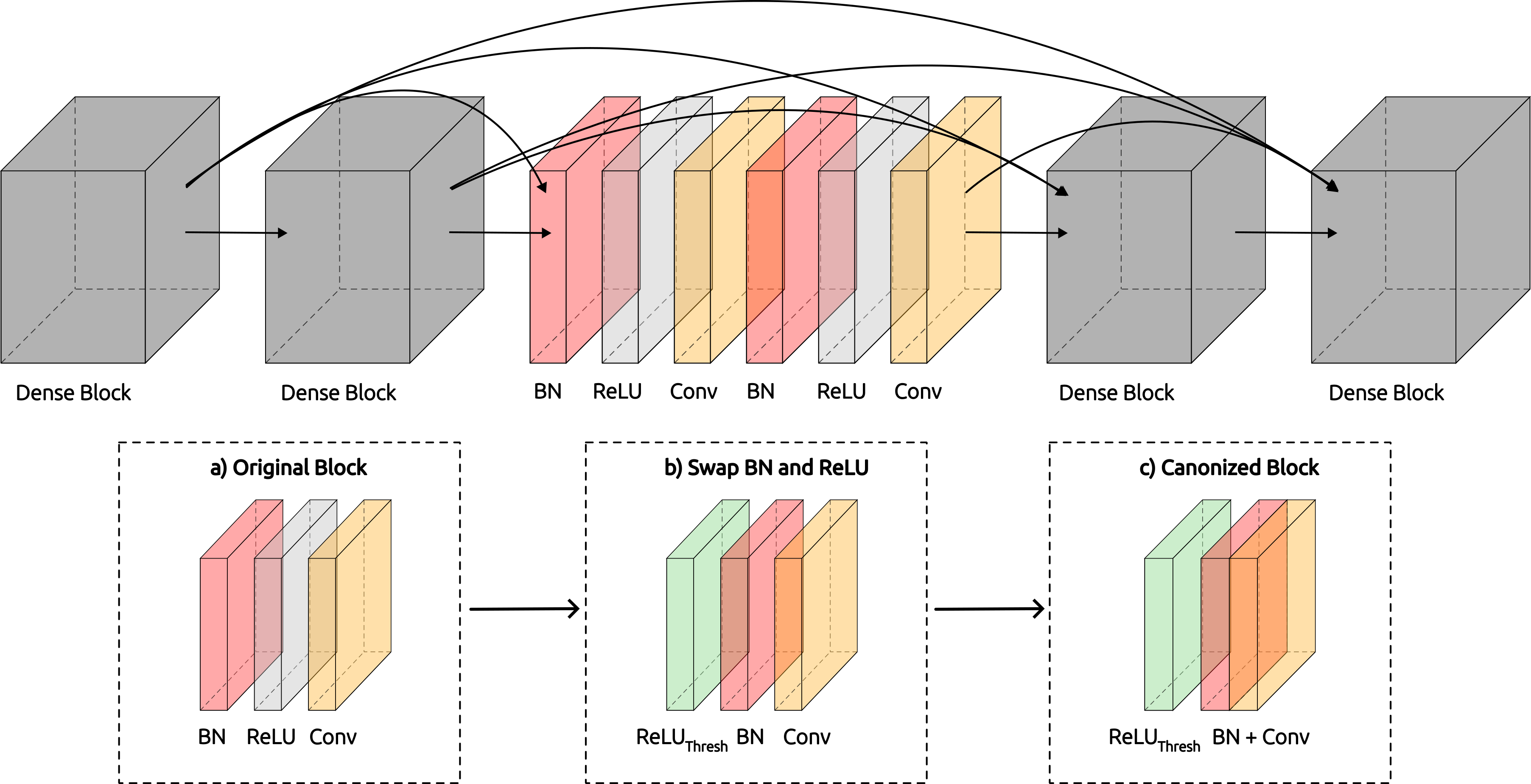
Figure 1: Due to the high interconnectivity of model components in DenseNets, it is not straightforward to fuse BN layers with Convolutional layers from neighboring blocks. Therefore, we suggest to first swap BN layers and ReLU activation functions using Eq. 7 (see step b)) and then merge the BN parameters into the following Convolutional layer using Eq. 6 (see step c)).

3.2 Canonization of Popular Architectures

We now demonstrate the canonization of popular neural network architectures. We picked 4 image classification models (VGG, ResNet, EfficientNet and DenseNet) and one VQA model (Relation Network [35]).

Image Classification Models:

Many popular image classification model architectures, such as VGG [44], ResNet [16] and EfficientNet [45], apply BN directly after linear layers. Therefore, these networks can easily be canonized using Eq. 4. It gets more complicated, however, if model architectures are more complex with highly interconnected building blocks. DenseNets, for example, use skip connections to pass activations from each dense block to all subsequent blocks, as shown in Fig. 1. Each block applies BN on the concatenated inputs coming from multiple blocks, followed by ReLU activation and a Convolutional layer (BN $\rightarrow$ ReLU $\rightarrow$ Conv). Note that due to the high interconnectivity, BN layers cannot easily be merged into linear layers from neighboring blocks, because most linear layers pass their activations to multiple blocks, and vice versa, most blocks receive activations from multiple blocks. Consequently, the linear transformation implementing the BN function has to be merged with the linear layer following the ReLU activation within the same block. Therefore, we propose to perform model canonization by first applying Eq. 7 and then Eq. 6 to join BN layers with following linear layers within the same block, over the ReLU function between them. This process is visualized in Fig. 1. In addition, we apply Eq. 4 to merge the first BN layer in the initial layers of the DenseNet architecture, before the dense blocks. Moreover, there is a BN$\rightarrow$ReLU$\rightarrow$AvgPool2d$\rightarrow$Conv chain in the end of the network, which can also be merged using Eq. 7 and Eq. 6.

VQA Model:

In contrast to image classification models, VQA models, e.g., Relation Network [35], require two paths to encode both, the input image and the input question. Relation Networks use a simple Convolutional neural network as image encoder. The implementation by the authors of CLEVR-XAI [4] applies BN after the activation function (Conv $\rightarrow$ ReLU $\rightarrow$ BN). Therefore, we merge BN layers with the Convolutional layer from the following block using Eq. 6. The BN layer of the last block of the image encoder has to be merged with the fully connected layer of the following module, which, however, receives a concatenation of image encoding and text encoding from the input question. Therefore, it has to be assured that BN parameters are merged only with the weights operating on inputs coming from the image encoder (see Section B and Fig. A.1 in the supplementary material for details).

4 Experiments: XAI Evaluation Framework

4.1 Datasets

ILSVRC2017 [33]

is a popular benchmark dataset for object recognition tasks with 1.2 million samples categorized into 1,000 classes, out of which we randomly picked 50 classes for our experiments (see Section E.1 in the supplementary material). Bounding box annotations are provided for a subset of ILSVRC2017, which we use for localization metrics. Per class, we use up to 640 random samples. Note that ILSVRC2017 faces a center-bias, i.e., most of the objects to be classified are located in the center of the image. Therefore, naive explainers can assume that models base their decisions on center pixels. To that end, we include additional experiments using the Pascal VOC 2012 dataset [13] in Section D in the supplementary material.

CLEVR-XAI [4]

builds upon the CLEVR dataset [22], which is an artificial VQA dataset. It contains 10,000 images showing objects with varying characteristics regarding shape, size, color and material. Moreover, there are simple and complex questions that need to be answered. The task is framed as a classification task, in which, given an image and a question, the model has to predict the correct response out of 28 possible answers. In total, there are approx. 40,000 simple questions, asking for certain characteristics of single objects. In addition, there are 100,000 complex questions, which require the understanding of relationships between multiple objects. CLEVR-XAI further comes with ground-truth explanations, encoded as binary masks locating the objects that are required in order to answer the question. Simple questions come with two binary masks, which are GT Single Object, localizing the object affected by the question, and GT All Objects, localizing all objects in the image. For complex questions there are four binary masks, including GT Union localizing all objects that are required to answer the question (we refer to [4] for details on the other masks).

4.2 Models

For our experiments with ILSVRC2017, we analyze VGG-16 [44], ResNet-18 [16], EfficientNet-B0 [45] and DenseNet-121 [19]. We use pre-trained models provided in the PyTorch model zoo [31]. We use a Relation Network [35] for our experiments with CLEVR-XAI.

4.3 XAI Methods and Implementation Details

We analyze rule-based and modified backpropagation based XAI methods , namely Excitation Backprop (EB) and LRP. Note that other backpropagation-based methods, such as Saliency, Smoothgrad, Integrated Gradients and Guided Backprop are not impacted by model canonization [30] and are therefore not analyzed in this experiment. For each method, we compute explanations for both, the original and the canonized model. We use zennit [2] as toolbox to compute explanations. For ILSVRC2017 with LRP, we analyze two pre-defined composites, i.e., mappings from layer type to LRP rule which have been established in literature [27], namely EpsilonPlus ($\varepsilon+$) and Alpha2-Beta1 ($\alpha$2$\beta$1), see Tab. A.1 in the supplementary material for details. For Relation Networks, we use a custom composite (LRP-Custom) following [4], in which we apply the $\alpha 1\beta 0$ rule to all linear layers and the box-rule [27] to the input layer. Note that ResNets, EfficientNets, and DenseNets leverage skip connections, which require the application of an additional canonizer in zennit to explicitly make them visible to the XAI method. Furthermore, we apply the signal-takes-it-all rule [3] to address the gate functions in the Squeeze-and-Excitation modules [18] in EfficientNets. In order to convert 3-dimensional relevance scores per voxel (channel $\times$ height $\times$ width) into 2-dimensional scores per pixel (height $\times$ width), we simply sum the relevances on the channel axis for ILSVRC2017 experiments. For CLEVR-XAI experiments we follow the authors from [4] and use pos-l2-norm-sq ($R_{\text{pool}}=\sum_{i=1}^{C}max(0,R_{i})^{2}$) as pooling function, where $C=3$ is the number of channels. Results for the alternative pooling function max-norm ($R_{\text{pool}}=max(|R_{1}|,R_{2},...,R_{C})$) are provided in the supplementary material. Moreover, before computing the metrics, we normalize the relevances by dividing all values by the square root of the second moment to bound their variance for numerical stability when comparing heatmaps.

4.4 XAI Metrics

In our experiments, we quantitatively measure the impact of canonization of the selected model architectures with various metrics, probing the quality of explanations from different viewpoints. We use the quantus toolbox [17] to compute the following metrics: We measure Faithfulness using Region Perturbation with blurring as baseline function. We compute the Area over Perturbation Curve (AoPC) [34] to measure the faithfulness in a single number as $\text{AoPC}=\frac{1}{L+1}\Big{(}\sum_{k=0}^{L}f(\textbf{x}^{(0)})-f(\textbf{x}^{(k)})\Big{)}$, where x is the input sample, $k$ is the perturbation step and $L$ is the total number of perturbations. The AoPC is averaged over all input samples. Localization quality is measured using RRA and RMA. As ground truth location we use bounding box annotations provided for ILSVRC2017, and binary segmentation masks for CLEVR-XAI. For the latter, we use GT Unique for simple questions and GT Union for complex questions. Moreover, we use the average sensitivity to measure Robustness, sparseness for Complexity and run the logit test as Randomization metric. While for robustness and randomization low scores are desirable, for the other metrics higher scores are better.

		$\uparrow$ Complexity		$\uparrow$ Faithfulness		$\uparrow$ Local. (RRA)		$\uparrow$ Local. (RMA)		$\downarrow$ Robustness		$\downarrow$ Random.
Model	canonized	no	yes	no	yes	no	yes	no	yes	no	yes	no	yes
VGG-16	EB	0.57	0.59	0.35	0.36	0.70	0.71	0.68	0.70	0.22	0.18	1.00	1.00
	LRP-$\alpha 2\beta 1$	0.70	0.84	0.38	0.39	0.63	0.67	0.65	0.77	0.31	0.34	0.59	0.66
	LRP-$\varepsilon$+	0.51	0.62	0.36	0.39	0.69	0.71	0.64	0.71	0.19	0.21	0.57	0.54
ResNet-18	EB	0.55	0.57	0.29	0.29	0.68	0.69	0.66	0.67	0.16	0.14	0.97	0.97
	LRP-$\alpha 2\beta 1$	0.67	0.76	0.32	0.32	0.65	0.67	0.69	0.75	0.21	0.26	0.65	0.61
	LRP-$\varepsilon$+	0.51	0.58	0.30	0.30	0.69	0.70	0.65	0.69	0.14	0.15	0.70	0.70
EfficientNet-B0	EB	0.85	0.70	0.24	0.27	0.73	0.67	0.79	0.72	0.42	0.33	0.99	1.00
	LRP-$\alpha 2\beta 1$	0.75	0.77	0.29	0.20	0.72	0.65	0.79	0.73	0.48	0.49	0.57	0.51
	LRP-$\varepsilon$+	0.50	0.73	0.28	0.30	0.75	0.75	0.69	0.79	0.12	0.21	0.61	0.65
DenseNet-121	EB	0.66	0.62	0.15	0.31	0.58	0.72	0.53	0.73	0.57	0.17	0.75	0.89
	LRP-$\alpha 2\beta 1$	0.82	0.81	0.25	0.33	0.64	0.71	0.68	0.81	0.65	0.28	0.40	0.44
	LRP-$\varepsilon$+	0.67	0.66	0.26	0.33	0.70	0.74	0.71	0.77	0.63	0.19	0.39	0.48

Table 1: XAI evaluation results with and without model canonization for VGG-16, ResNet-18, EfficientNet-B0 and DenseNet-121 using the ILSVRC2017 dataset. We measure the quality of explanations using the metrics Sparseness (Complexity), Region Perturbation (Faithfulness), RRA and RMA (Localization), Avg. Sensitivity (Robustness) and Random Logit Test (Randomization). Arrows indicate whether high ($\uparrow$) or low ($\downarrow$) are better. Best results are shown in bold.

		$\uparrow$ Complexity		$\uparrow$ Faithfulness		$\uparrow$ Local. (RRA)		$\uparrow$ Local. (RMA)		$\downarrow$ Robustness		$\downarrow$ Random.
Questions	canonized	no	yes	no	yes	no	yes	no	yes	no	yes	no	yes
Simple	EB	0.99	0.97	0.50	0.51	0.64	0.61	0.76	0.70	1.37	1.39	1.00	1.0
	LRP-Custom [4]	0.95	0.98	0.52	0.52	0.70	0.70	0.75	0.83	1.33	1.35	0.99	1.0
Complex	EB	0.99	0.97	0.44	0.45	0.66	0.62	0.82	0.77	1.36	1.35	1.00	0.99
	LRP-Custom [4]	0.94	0.97	0.45	0.46	0.54	0.63	0.79	0.86	1.33	1.34	0.98	0.99

Table 2: XAI evaluation results for Relation Network with and without model canonization using the CLEVR-XAI dataset for simple and complex questions using pos-l2-norm-sq-pooling. Arrows indicate whether high ($\uparrow$) or low ($\downarrow$) are better. Best results are shown in bold.

4.5 Canonization Results

The XAI evaluation results for the ILSVRC2017 dataset comparing models with and without canonization using the metrics described above are shown in Tab. 1. It can be seen that for most models and metrics the XAI methods yield better explanations for canonized models, especially for complexity, faithfulness, and localization metrics. However, there are some exceptions. While all other models yield less complex explanations when using model canonization, DenseNet explanations show the opposite behavior. This is due to the fact that many explanation heatmaps for DenseNets focus on small pixel groups (see Fig. A.7 in supplementary material) that, however, do not truly represent the model’s behavior, as low faithfulness scores without canonization indicate. The localization metrics tend to be better for canonized models, except for EfficientNet-B0 with the $\alpha 2\beta 1$-composite for LRP, which, however, also yields a poor performance in terms of faithfulness. Hence, the $\alpha 2\beta 1$-composite itself appears to be a suboptimal parameterization for EfficientNets, which demonstrates the importance of the choice of hyperparameters for rule-based XAI methods. Note that randomization scores tend to increase for canonized models, i.e., the canonized model leads to explanations that are less dependent on the target class. This is due to the fact that the explanations are more focused on the object to classify (see improvements for localization metrics in Tab. 1) and therefore are more similar when computed for different target classes. Hence, randomization metrics have to be interpreted with caution [8]. Results for additional models and XAI evaluation metrics are shown in the supplementary material in Tables A.9-A.15.

In Tab. 2 we show results for our XAI evaluation using the CLEVR-XAI dataset. For LRP-Custom, model canonization yields explanations that are either better than those of the original model or approximately on par with them for both simple and complex questions, in particular for localization metrics. Results with max-norm-pooling are shown in the supplementary material in Tab. A.16.

Figure 2: Results Grid Search for VGG-13: We group the layers into low-level (Conv 1-3), mid-level (Conv 4-7) and high-level (Conv 8-10) Convolutions, as well as fully connected layers in the classification head (Classifier). We evaluate different parameterizations for the $\gamma$-rule, where we define different values for $\gamma$ per group and measure the quality of explanations both with and without model canonization w.r.t localization, faithfulness, complexity, randomization and robustness metrics.

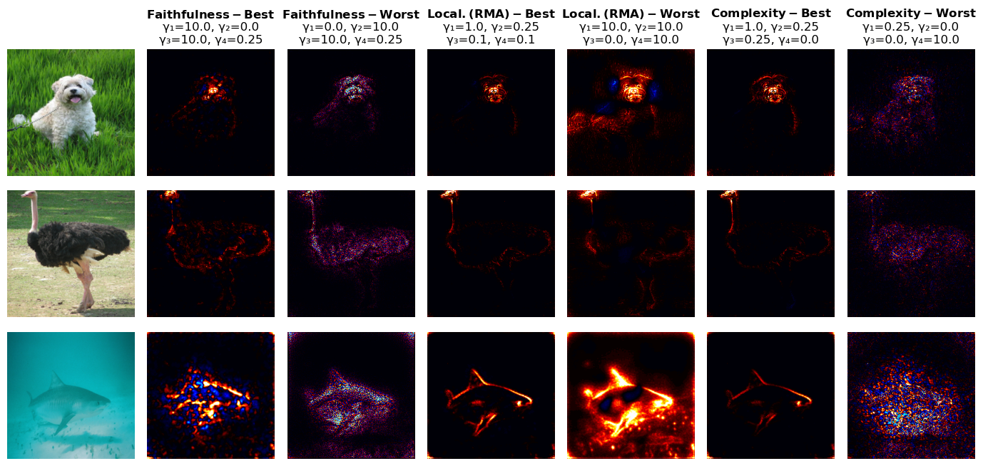
Figure 3: Attribution heatmaps (with canonization) for best and worst $\gamma$-parameters according to the grid search. $\gamma_{1}$ is for low-level features (Conv 1-4), $\gamma_{2}$ is for mid-level features (Conv 5-10), $\gamma_{3}$ is for high-level features (Conv 10-13), $\gamma_{4}$ is for layers in the classification head.

4.6 XAI Hyperparameter Tuning

For our experiments in Section 4.5 we used pre-defined LRP composites established in literature [27, 23]. However, as suggested by different results for evaluated composites, these parameters differently impact the quality of explanations w.r.t the chosen metric. To that end, we run another experiment that uses our XAI evaluation framework for hyperparameter search. Specifically, we focus on the LRP-$\gamma$-rule, which uses the parameter $\gamma$ to regulate the effect of positive and negative contributions (see Sec. 2.3), ranging from treating both equally ($\gamma=0$) to neglecting negative contributions ($\gamma\rightarrow\infty$). Further, the flexibility of the LRP framework allows us to define XAI methods with varying focus on positive and negative contributions depending on the position of the layer in the network. We use a VGG-13 model with BN and define 4 groups of network layers, which are low-level (Conv 1-3), mid-level (Conv 4-7), and high-level (Conv 8-10) layers, as well as fully-connected layers in the classification head. We define one $\gamma$-parameter per group with $\gamma\in\{0,0.1,0.25,0.5,1,10\}$, and run a grid search for all possible combinations with and without model canonization, i.e., $2\cdot 6^{4}=2592$ $\gamma$-configurations. Note that in theory, we could also evaluate different sub-canonizations, where we only canonize certain parts of the model. This, however, further increases the degrees of freedom. Further note that more advanced multi-metric-objective hyperparameter optimization approaches can be employed. However, we decided to go forward with simple grid search, because our goal is to highlight the importance of the choice of XAI hyperparameters and the impact on various evaluation metrics. We evaluate the resulting explanations with the metrics described in section 4.4 and show the results in Fig. 2. Specifically, each line represents the score per metric with $\gamma$ for a certain group of layers kept constant, averaged over all $\gamma$-parameterizations for other layer groups. It can be seen that the impact of the choice of $\gamma$ depends on the position of the layer in the network and, in addition, differs by the metric of choice. For instance, the robustness of the explanations is mainly impacted by the $\gamma$-value in low-level layers (Conv 1-3), while it has no impact for the other layers. In contrast, randomization is mostly impacted by the choice of $\gamma$ for fully connected layers in the classification head. Interestingly, canonization has a large impact on the optimal choice of $\gamma$ for low-level layers when measuring the faithfulness of the resulting explanations. In Fig. 3 we show attribution heatmaps for three samples using different $\gamma$-configurations, employing the best and worst parameterization according to the metrics faithfulness, localization and complexity. Each metric favors another parametrization, leading to different attribution heatmaps. High $\gamma$-values in low-level layers ($\gamma_{1}$) appear to be favorable for all metrics, i.e., more focus on positive contributions on those layers. This leads to attribution heatmaps with less noise, which is beneficial w.r.t faithfulness, localization and complexity.

5 Conclusions

In this work, we proposed an evaluation framework for XAI methods which can be leveraged to optimize the quality of explanations based on a variety of XAI metrics. Specifically, we demonstrated the application of our framework to measure the impact of model canonization towards various aspects of explanation quality. Therefore, we extended the model canonization approach to state-of-the-art model architectures, including EfficientNets and DenseNets. Despite not always being beneficial w.r.t. all examined architectures, model canonization provides an extra option when adopting XAI methods to the task at hand. Moreover, we applied our evaluation framework for hyperparameter optimization for XAI methods and demonstrated the impact of parameters w.r.t different XAI metrics. While we have evaluated our methods for LRP, it is also applicable to other configurable XAI methods, such as DeepLift. Future work will focus on the canonization of additional relevant model architectures, e.g., Vision Transformer [12]. In addition, optimizing the hyperparameter search is an promising research direction, e.g., with random search, evolutionary algorithms, or other approaches to reduce the search space. Moreover, the framework can be applied with other optimization objectives, e.g., to find LRP configurations that mimic other, more expensive XAI methods, e.g., SHAP.

Appendix A Canonization Details

Linear $\rightarrow$ BN:

In Eqs. (A.1) - (A.5), we show more detailed steps required to fuse Linear $\rightarrow$ BN components into a single affine transformation, as outlined in Eq. (4) in the main paper:

$$f(\textbf{x}) =\text{BN}(\text{Linear}(\textbf{x}))$$ (A.1)

$$=\text{BN}(w_{L}^{\top}\textbf{x}+b_{L})$$ (A.2)

$$=w_{BN}\Big{(}\frac{w_{L}^{\top}\textbf{x}+b_{L}-\mu}{\sqrt{\sigma+\epsilon}}\Big{)}+b_{BN}$$ (A.3)

$$=\frac{w_{BN}}{\sqrt{\sigma+\epsilon}}(w_{L}^{\top}\textbf{x}+b_{L}-\mu)+b_{BN}$$ (A.4)

$$=(\underbrace{\frac{w_{BN}}{\sqrt{\sigma+\epsilon}}w_{L}}_{w_{\text{new}}})^{\top}\textbf{x}+\underbrace{\frac{w_{BN}}{\sqrt{\sigma+\epsilon}}(b_{L}-\mu)+b_{BN}}_{b_{\text{new}}}$$ (A.5)

BN $\rightarrow$ Linear:

In Eqs. (A.6) - (A.9), we show more detailed steps required to fuse BN $\rightarrow$ Linear component chains into a single affine transformation, as outlined in Eq. (6) in the main paper:

$$f(\textbf{x}) =\text{Linear}(\text{BN}(\textbf{x}))$$ (A.6)

$$=w_{L}^{\top}\Bigg{(}w_{BN}\Big{(}\frac{\textbf{x}-\mu}{\sqrt{\sigma+\epsilon}}\Big{)}+b_{BN}\Bigg{)}+b_{L}$$ (A.7)

$$=w_{L}^{\top}\Big{(}\frac{w_{BN}\textbf{x}-w_{BN}\mu}{\sqrt{\sigma+\epsilon}}+b_{BN}\Big{)}+b_{L}$$ (A.8)

$$=\underbrace{\frac{w_{L}^{\top}w_{BN}}{\sqrt{\sigma+\epsilon}}}_{w_{\text{new}}}\textbf{x}\underbrace{-\frac{w_{L}^{\top}w_{BN}\mu}{\sqrt{\sigma+\epsilon}}+w_{L}^{\top}b_{BN}+b_{L}}_{b_{\text{new}}}$$ (A.9)

Padding Issue in BN $\rightarrow$ Linear Canonization: If the linear layer is a Convolutional layer with constant valued padding, the bias of the linear layer after canonization can no longer be shown as a scalar:

$$f(\textbf{x}) =\text{Conv$($Pad$($BN$(${x}})))$$ (A.10)

$$=\text{Conv$($Pad$($}\frac{w_{BN}}{\sqrt{\sigma+\epsilon}}\textbf{x}-\frac{w_{BN}\mu}{\sqrt{\mu+\epsilon}}+b_{BN}))$$ (A.11)

$$=\text{Conv(}\frac{w_{BN}}{\sqrt{\sigma+\epsilon}}\text{Pad}(\textbf{x})+\text{Pad}(-\frac{w_{BN}\mu}{\sqrt{\sigma+\epsilon}}+b_{BN}))$$ (A.12)

$$=w_{L}\ast\Big{(}\frac{w_{BN}}{\sqrt{\sigma+\epsilon}}\text{Pad}(\textbf{x})+\text{Pad}(-\frac{w_{BN}\mu}{\sqrt{\sigma+\epsilon}}+b_{BN})\Big{)}$$

$$\qquad\qquad\qquad\qquad\qquad\qquad\qquad\qquad\quad\enspace+b_{L}$$ (A.13)

$$\begin{aligned} =\Big{(}w_{L}^{\top}\frac{w_{BN}}{\sqrt{\sigma+\epsilon}}\Big{)}&\ast\text{Pad}(\textbf{x})\\ +w_{L}&\ast\text{Pad}(-\frac{w_{BN}\mu}{\sqrt{\sigma+\epsilon}}+b_{BN})+b_{L}\end{aligned}$$ (A.14)

$$\begin{aligned} =\underbrace{\Big{(}w_{L}^{\top}\frac{w_{BN}}{\sqrt{\sigma+\epsilon}}\Big{)}}_{w_{\text{new}}}&\ast\text{Pad}(\textbf{x})\\ &+\underbrace{\text{Conv}(\text{Pad}(-\frac{w_{BN}\mu}{\sqrt{\sigma+\epsilon}}+b_{BN}))}_{b_{\text{new}}}\end{aligned}$$ (A.15)

In the equations above, $\ast$ stands for convolution. The new bias term is a full feature map, as opposed to a scalar as in linear layers without padding. The feature map does not depend on input x and is computed by putting a feature map (of the same size as x) with all features equal to $-\frac{w_{BN}\mu}{\sqrt{\sigma+\epsilon}}+b_{BN}$ through the original linear layer. Notice that if the padding value is nonzero, then the padding value of the canonized layer must be scaled by $\frac{\sqrt{\sigma+\epsilon}}{w_{BN}}$

We now give a simple example to help illustrate the problem and the proposed solution. Specifically, we set BN parameters $\mu=0,\sigma=1,\epsilon=0,w_{\text{BN}}=1,b_{\text{BN}}=1$. Furthermore we define a single Convolutional filter with zero padding of width 1, $w_{L}=\begin{bmatrix}1&1\\ 1&1\end{bmatrix}$ and no bias, $b_{L}=0$. Finally, we choose to show the case of a simple $3\times 3$ input feature map

x $$=\begin{bmatrix}1&2&3\\ 2&3&4\\ 3&4&5\end{bmatrix}$$ (A.16)

$$Pad(BN(\textbf{x})) =\begin{bmatrix}0&0&0&0&0\\ 0&2&3&4&0\\ 0&3&4&5&0\\ 0&4&5&6&0\\ 0&0&0&0&0\end{bmatrix}$$ (A.17)

$$w_{L}\ast Pad(BN(\textbf{x})) =\begin{bmatrix}2&5&7&4\\ 5&12&16&9\\ 7&16&20&11\\ 4&9&11&6\end{bmatrix}$$ (A.18)

$$=\begin{bmatrix}1&3&5&3\\ 3&8&12&7\\ 5&12&16&9\\ 3&7&9&5\end{bmatrix} +\begin{bmatrix}1&2&2&1\\ 2&4&4&2\\ 2&4&4&2\\ 1&2&2&1\end{bmatrix}$$ (A.19)

$$=w_{\text{new}}\ast Pad(\textbf{x}) +w_{L}\ast Pad(BNBias)+b_{L}$$ (A.20)

where and $BNBias=\begin{bmatrix}1&1&1\\ 1&1&1\\ 1&1&1\end{bmatrix}$ is the feature map composed of values equal to $-\frac{w_{BN}\mu}{\sqrt{\sigma+\epsilon}}+b_{BN}$

Appendix B Canonization of Relation Networks

Architecture:

Relation Networks [35] are the state-of-the-art model architecture for the CLEVR dataset. It uses two separate encoders for image and text input. For the image, a simple convolutional neural network is used with 4 blocks, each containing a Convolutional layer, followed by a ReLU activation function and a BN layer. The text input is processed by a LSTM. The pixels from the feature map from the last Convolutional block from the image encoder are pair-wise concatenated along with their coordinates and the text encoding. This representation is then passed to a 4-layer fully connected network, summed up and then processed by a 3-layer fully connected network with ReLU activation.

Canonization:

Relation Networks, as implemented by the authors of [4], use BN layers at the end of each block not directly after Convolutional layers. Therefore, we suggest to merge the BN layers with the Convolutional layers at the beginning of the following block. The BN layer of the last block of the image encoder can be merged into the following fully connected layer. However, attention as to be paid to make sure only weights operating on activations coming from the image encoder are updated, as outlined below. The proposed canonization of Relation Networks is visualized in Fig. A.1

Challenge:

In relation networks, the last BN layer of the image encoder has to be merged into a linear layer of the succeeding block, which takes as input a concatenation of image pairs, text and indices. Therefore, only the weights responsible for the activations coming from the image encoder have to be updated.

Incoming Activations:

$$\textbf{x}=\text{concat}\overbrace{\Big{[}\underbrace{[\textbf{x1}]}_{24},\underbrace{[\text{coord1}]}_{2},\underbrace{[\textbf{x2}]}_{24},\underbrace{[\text{coord2}]}_{2},\underbrace{[\text{question}]}_{128}\Big{]}}^{180}$$ (A.21)

Only x1 and x2 pass the BN layer, i.e., indices $0:24$ and $26:50$ have to be updated. Here, the indexing $i:j$ signifies the elements with indices from $i$ to $j-1$, where the first element is indexed with $0$. In order to update only the relevant part of the weights of the linear layer $w_{L}$, we have to split them into:

$$w_{L}=\text{concat}\Big{[}\underbrace{[w_{L}^{0:24}]}_{\textbf{x1}},\underbrace{[w_{L}^{24:26}]}_{\text{coord1}},\underbrace{[w_{L}^{26:50}]}_{\textbf{x2}},\underbrace{[w_{L}^{50:52}]}_{\text{coord2}},\underbrace{[w_{L}^{52:180}]}_{\text{text}}\Big{]}$$ (A.22)

Using Eq. (A.9), each relevant weight part can than be updated as follows:

$$w_{L_{\text{new}}}^{0:24}=\frac{{w_{L}^{0:24}}^{\top}w_{BN}}{\sqrt{\sigma+\epsilon}}$$ (A.23)

$$w_{L_{\text{new}}}^{26:50}=\frac{{w_{L}^{26:50}}^{\top}w_{BN}}{\sqrt{\sigma+\epsilon}}$$ (A.24)

This gives a new weight matrix:

$$w_{L_{\text{new}}}=\text{concat}\Big{[}\underbrace{[w_{L_{\text{new}}}^{0:24}]}_{\textbf{x1}},\underbrace{[w_{L}^{24:26}]}_{\text{coord1}},\underbrace{[w_{L_{\text{new}}}^{26:50}]}_{\textbf{x2}},\underbrace{[w_{L}^{50:52}]}_{\text{coord2}},\underbrace{[w_{L}^{52:180}]}_{\text{text}}\Big{]}$$ (A.25)

Similarly, the new bias can be calculated as:

$$b_{L_{\text{new}}}=w_{L}^{0:24}b_{\text{linBN}}+w_{L}^{26:50}b_{\text{linBN}}+b_{C}$$ (A.26)

with $b_{\text{linBN}}=b_{BN}-\frac{w_{B}N\cdot\mu}{\sqrt{\sigma+\epsilon}}$

Figure A.1: Canonization of Relation Network. (Left): Part from the original Relation Network. (Right): Suggested canonization for the corresponding part of Relation Networks. BN layers are merged into the Convolutional layer at the beginning of the following block. The BN layer of the last block is merged into the following fully connected layer. However, only weights operating upon activations coming from the image encoder are updated, as outlined in Eq. (A.25).

Appendix C Composites

The composites, i.e., pre-defined layer-to-rule assignments as suggested in the literature, that we used in the paper, are described in Tab. A.1.

Composite	Layer Type	Rule
LRP-$\epsilon+$	Convolutional	$\alpha 1\beta 0$-rule
	Fully Connected	$\epsilon$-rule
LRP-$\alpha 2\beta 1$	Convolutional	$\alpha 2\beta 1$-rule
	Fully Connected	$\epsilon$-rule
LRP-Custom (RN)	First Convolutional	box-rule
	Other Convolutionals	$\alpha 1\beta 0$-rule
	Fully Connected	$\alpha 1\beta 0$-rule

Table A.1: Details for composites used in our experiments.

Appendix D Pascal VOC 2012 Experiments

D.1 Dataset Description

Pascal Visual Object Classes (VOC) 2012 dataset has images from 20 categories, including 5717 training samples and 5823 validation samples with bounding box annotations, along with a private test set. From those, 1464 training samples and 1449 validation samples are annotated with binary segmentation masks. As opposed to ILSVRC2017, the images are much more diverse in composition. Many images contain multiple instances of several categories. The dataset does not suffer from the center-bias mentioned for ILSVRC2017. In the experiments, we use the validation samples with segmentation masks. Due to the robustness of models to input perturbations, the faithfulness correlation scores are very low, even entirely zero for some models. In order to obtain more meaningful results, we report faithfulness correlation scores with bigger perturbations compared to the ILSVRC2017 experiments.

D.2 Models

We evaluate explanations on VGG-16, ResNet-18, ResNet-50, EfficientNet-B0, EfficientNet-B4, DenseNet-121 and DenseNet-161. We fine tune models using the full training set, using pre-trained models from the PyTorch model zoo. We use stochastic gradient descent as the learning algorithm, with a cosine annealing learning rate scheduler [24]. We use sum of binary cross entropy losses as the loss, and train the networks until convergence. We opted to use a smaller learning rate for pretrained parameters.

D.3 Results

The results are shown in Tables A.2 - A.8. The results suggest that canonization increases performance in the localization metrics and partially for faithfulness metrics. For the robustness metrics, canonization helps for Excitation Backpropagation. However, it makes robustness scores improve by a bigger margin for all methods for DenseNet models. Similar to the results for ILSVRC2017, DenseNet models seem to be affected negatively in their complexity scores when canonized. For other model architectures, complexity measures are also uniformly improved by canonization.

	Complexity		Faithfulness				Localization				Random.		Robustness
	$\uparrow$ Spars.		$\uparrow$ Corr.		$\uparrow$ AoPC		$\uparrow$ RMA		$\uparrow$ RRA		$\downarrow$ Logit		$\downarrow$ Avg. Sens.		$\downarrow$ Max Sens.
canonized	no	yes	no	yes	no	yes	no	yes	no	yes	no	yes	no	yes	no	yes
EB	0.59	0.60	0.04	0.04	0.21	0.22	0.33	0.34	0.40	0.41	1.00	1.00	0.24	0.20	0.26	0.21
LRP-$\alpha 2\beta 1$	0.75	0.86	0.04	0.03	0.27	0.27	0.38	0.44	0.40	0.41	0.53	0.64	0.53	0.53	0.80	0.78
LRP-$\varepsilon$+	0.59	0.68	0.05	0.05	0.25	0.26	0.36	0.40	0.46	0.47	0.49	0.49	0.51	0.51	0.80	0.78

Table A.2: Results for Pascal VOC XAI evaluation with VGG-16. Arrows indicate whether high ($\uparrow$) or low ($\downarrow$) are better. Best results are shown in bold.

	Complexity		Faithfulness				Localization				Random.		Robustness
	$\uparrow$ Spars.		$\uparrow$ Corr.		$\uparrow$ AoPC		$\uparrow$ RMA		$\uparrow$ RRA		$\downarrow$ Logit		$\downarrow$ Avg. Sens.		$\downarrow$ Max Sens.
canonized	no	yes	no	yes	no	yes	no	yes	no	yes	no	yes	no	yes	no	yes
EB	0.53	0.57	0.03	0.04	0.22	0.23	0.31	0.33	0.40	0.41	0.96	0.97	0.17	0.15	0.19	0.16
LRP-$\alpha 2\beta 1$	0.70	0.77	0.03	0.03	0.23	0.23	0.34	0.39	0.36	0.39	0.65	0.64	0.48	0.48	0.77	0.77
LRP-$\varepsilon$+	0.56	0.63	0.03	0.03	0.22	0.22	0.31	0.34	0.39	0.41	0.68	0.68	0.46	0.45	0.77	0.76

Table A.3: Results for Pascal VOC XAI evaluation with ResNet-18. Arrows indicate whether high ($\uparrow$) or low ($\downarrow$) are better. Best results are shown in bold.

	Complexity		Faithfulness				Localization				Random.		Robustness
	$\uparrow$ Spars.		$\uparrow$ Corr.		$\uparrow$ AoPC		$\uparrow$ RMA		$\uparrow$ RRA		$\downarrow$ Logit		$\downarrow$ Avg. Sens.		$\downarrow$ Max Sens.
canonized	no	yes	no	yes	no	yes	no	yes	no	yes	no	yes	no	yes	no	yes
EB	0.55	0.63	0.04	0.04	0.20	0.23	0.30	0.35	0.38	0.42	0.96	0.93	0.20	0.17	0.21	0.18
LRP-$\alpha 2\beta 1$	0.73	0.81	0.03	0.03	0.24	0.24	0.38	0.41	0.39	0.39	0.60	0.62	0.48	0.49	0.74	0.73
LRP-$\varepsilon$+	0.60	0.69	0.04	0.04	0.24	0.25	0.35	0.39	0.44	0.44	0.60	0.57	0.46	0.46	0.75	0.74

Table A.4: Results for Pascal VOC XAI evaluation with ResNet-50. Arrows indicate whether high ($\uparrow$) or low ($\downarrow$) are better. Best results are shown in bold.

	Complexity		Faithfulness				Localization				Random.		Robustness
	$\uparrow$ Spars.		$\uparrow$ Corr.		$\uparrow$ AoPC		$\uparrow$ RMA		$\uparrow$ RRA		$\downarrow$ Logit		$\downarrow$ Avg. Sens.		$\downarrow$ Max Sens.
canonized	no	yes	no	yes	no	yes	no	yes	no	yes	no	yes	no	yes	no	yes
EB	0.55	0.69	0.01	0.02	0.13	0.18	0.26	0.37	0.30	0.41	1.00	0.99	0.43	0.39	0.50	0.43
LRP-$\alpha 2\beta 1$	0.73	0.76	0.00	0.00	0.18	0.11	0.37	0.34	0.39	0.34	0.63	0.51	0.58	0.58	0.80	0.79
LRP-$\varepsilon$+	0.51	0.72	0.02	0.02	0.17	0.19	0.30	0.39	0.41	0.43	0.59	0.67	0.46	0.49	0.77	0.77

Table A.5: Results for Pascal VOC XAI evaluation with EfficientNet-B0. Arrows indicate whether high ($\uparrow$) or low ($\downarrow$) are better. Best results are shown in bold.

	Complexity		Faithfulness				Localization				Random.		Robustness
	$\uparrow$ Spars.		$\uparrow$ Corr.		$\uparrow$ AoPC		$\uparrow$ RMA		$\uparrow$ RRA		$\downarrow$ Logit		$\downarrow$ Avg. Sens.		$\downarrow$ Max Sens.
canonized	no	yes	no	yes	no	yes	no	yes	no	yes	no	yes	no	yes	no	yes
EB	0.68	0.77	0.0	0.0	0.14	0.13	0.33	0.36	0.37	0.37	0.97	1.00	0.32	0.36	0.37	0.43
LRP-$\alpha 2\beta 1$	0.71	0.75	0.0	0.0	0.12	0.08	0.27	0.32	0.31	0.33	0.46	0.42	0.62	0.61	0.93	0.91
LRP-$\varepsilon$+	0.54	0.77	0.0	0.0	0.15	0.16	0.28	0.40	0.36	0.42	0.51	0.57	0.51	0.51	0.88	0.85

Table A.6: Results for Pascal VOC XAI evaluation with EfficientNet-B4. Arrows indicate whether high ($\uparrow$) or low ($\downarrow$) are better. Best results are shown in bold.

	Complexity		Faithfulness				Localization				Random.		Robustness
	$\uparrow$ Spars.		$\uparrow$ Corr.		$\uparrow$ AoPC		$\uparrow$ RMA		$\uparrow$ RRA		$\downarrow$ Logit		$\downarrow$ Avg. Sens.		$\downarrow$ Max Sens.
canonized	no	yes	no	yes	no	yes	no	yes	no	yes	no	yes	no	yes	no	yes
EB	0.63	0.59	0.02	0.04	0.11	0.25	0.25	0.37	0.28	0.48	0.98	0.75	0.60	0.20	1.07	0.22
LRP-$\varepsilon$+	0.70	0.63	0.02	0.04	0.18	0.24	0.34	0.36	0.39	0.44	0.35	0.44	0.63	0.50	1.08	0.77
LRP-$\alpha 2\beta 1$	0.83	0.73	0.01	0.03	0.16	0.24	0.31	0.39	0.32	0.41	0.38	0.36	0.64	0.51	1.11	0.76

Table A.7: Results for Pascal VOC XAI evaluation with DenseNet-121. Arrows indicate whether high ($\uparrow$) or low ($\downarrow$) are better. Best results are shown in bold.

	Complexity		Faithfulness				Localization				Random.		Robustness
	$\uparrow$ Spars.		$\uparrow$ Corr.		$\uparrow$ AoPC		$\uparrow$ RMA		$\uparrow$ RRA		$\downarrow$ Logit		$\downarrow$ Avg. Sens.		$\downarrow$ Max Sens.
canonized	no	yes	no	yes	no	yes	no	yes	no	yes	no	yes	no	yes	no	yes
EB	0.80	0.58	0.01	0.05	0.05	0.23	0.11	0.35	0.17	0.47	0.99	0.77	0.57	0.19	0.84	0.21
LRP-$\varepsilon$+	0.67	0.63	0.02	0.05	0.17	0.22	0.34	0.36	0.40	0.44	0.32	0.49	0.62	0.48	1.06	0.74
LRP-$\alpha 2\beta 1$	0.82	0.74	0.01	0.03	0.16	0.21	0.31	0.39	0.33	0.41	0.52	0.45	0.64	0.50	1.13	0.74

Table A.8: Results for Pascal VOC XAI evaluation with DenseNet-161. Arrows indicate whether high ($\uparrow$) or low ($\downarrow$) are better. Best results are shown in bold.

Appendix E ILSVRC2017 Experiments

E.1 Classes

In our experiments we considered the following 50 classes that were picked randomly:

“Bernese_mountain_dog”, “Christmas_stocking”, “Gila_monster”, “Shetland_sheepdog”, “Windsor_tie”, “amphibian”, “ant”, “bubble”, “cassette”, “cicada”, “collie”, “crossword_puzzle”, “dalmatian”, “eft”, “file”, “flute”, “goldfish”, “gorilla”, “gown”, “grasshopper”, “green_snake”, “gyromitra”, “hammer”, “hen_of_the_woods”, “indigo_bunting”, “kimono”, “magnetic_compass”, “mongoose”, “mountain_tent”, “otterhound”, “palace”, “patio”, “pencil_sharpener”, “platypus”, “pomegranate”, “pool_table”, “redshank”, “refrigerator”, “rhinoceros_beetle”, “screw”, “screwdriver”, “shoe_shop”, “shopping_basket”, “stage”, “standard_poodle”, “stethoscope”, “toaster”, “tree_frog”, “vase”, “wolf_spider”.

E.2 Additional Results

In Tables A.9 - A.15 we show additional results for our experiments with the ILSVRC2017 dataset. Specifically, in addition to the architectures evaluated in the main paper, we present results for ResNet50, EfficientNet-B4 and DenseNet-161. Moreover, we include results for Faithfulness Correlation [7] and Max Sensitivity [48].

	Complexity		Faithfulness				Localization				Random.		Robustness
	$\uparrow$ Spars.		$\uparrow$ Corr.		$\uparrow$ AoPC		$\uparrow$ RMA		$\uparrow$ RRA		$\downarrow$ Logit		$\downarrow$ Avg. Sens.		$\downarrow$ Max Sens.
canonized	no	yes	no	yes	no	yes	no	yes	no	yes	no	yes	no	yes	no	yes
EB	0.57	0.59	0.06	0.06	0.35	0.36	0.68	0.70	0.70	0.71	1.00	1.00	0.22	0.18	0.23	0.20
LRP-$\alpha 2\beta 1$	0.70	0.84	0.05	0.03	0.38	0.39	0.65	0.77	0.63	0.67	0.59	0.66	0.31	0.34	0.34	0.37
LRP-$\varepsilon$+	0.51	0.62	0.09	0.08	0.36	0.39	0.64	0.71	0.69	0.71	0.57	0.54	0.19	0.21	0.21	0.24

Table A.9: Results for ILSVRC2017 XAI evaluation with VGG-16. Arrows indicate whether high ($\uparrow$) or low ($\downarrow$) are better. Best results are shown in bold.

	Complexity		Faithfulness				Localization				Random.		Robustness
	$\uparrow$ Spars.		$\uparrow$ Corr.		$\uparrow$ AoPC		$\uparrow$ RMA		$\uparrow$ RRA		$\downarrow$ Logit		$\downarrow$ Avg. Sens.		$\downarrow$ Max Sens.
canonized	no	yes	no	yes	no	yes	no	yes	no	yes	no	yes	no	yes	no	yes
EB	0.55	0.57	0.03	0.04	0.29	0.29	0.66	0.67	0.68	0.69	0.97	0.97	0.16	0.14	0.18	0.15
LRP-$\alpha 2\beta 1$	0.67	0.76	0.04	0.03	0.32	0.32	0.69	0.75	0.65	0.67	0.65	0.61	0.21	0.26	0.22	0.28
LRP-$\varepsilon$+	0.51	0.58	0.04	0.04	0.30	0.30	0.65	0.69	0.69	0.70	0.70	0.70	0.14	0.15	0.15	0.16

Table A.10: Results for ILSVRC2017 XAI evaluation with ResNet-18. Arrows indicate whether high ($\uparrow$) or low ($\downarrow$) are better. Best results are shown in bold.

	Complexity		Faithfulness				Localization				Random.		Robustness
	$\uparrow$ Spars.		$\uparrow$ Corr.		$\uparrow$ AoPC		$\uparrow$ RMA		$\uparrow$ RRA		$\downarrow$ Logit		$\downarrow$ Avg. Sens.		$\downarrow$ Max Sens.
canonized	no	yes	no	yes	no	yes	no	yes	no	yes	no	yes	no	yes	no	yes
EB	0.72	0.64	0.02	0.04	0.24	0.36	0.65	0.71	0.66	0.69	0.95	0.93	0.36	0.17	0.42	0.18
LRP-$\alpha 2\beta 1$	0.71	0.81	0.04	0.01	0.37	0.37	0.72	0.77	0.66	0.67	0.59	0.61	0.25	0.30	0.27	0.33
LRP-$\varepsilon$+	0.57	0.67	0.05	0.04	0.37	0.37	0.70	0.74	0.72	0.71	0.61	0.60	0.15	0.18	0.16	0.19

Table A.11: Results for ILSVRC2017 XAI evaluation with ResNet-50. Arrows indicate whether high ($\uparrow$) or low ($\downarrow$) are better. Best results are shown in bold.

	Complexity		Faithfulness				Localization				Random.		Robustness
	$\uparrow$ Spars.		$\uparrow$ Corr.		$\uparrow$ AoPC		$\uparrow$ RMA		$\uparrow$ RRA		$\downarrow$ Logit		$\downarrow$ Avg. Sens.		$\downarrow$ Max Sens.
canonized	no	yes	no	yes	no	yes	no	yes	no	yes	no	yes	no	yes	no	yes
EB	0.85	0.70	0.00	0.0	0.24	0.27	0.79	0.72	0.73	0.67	0.99	1.00	0.42	0.33	0.48	0.37
LRP-$\alpha 2\beta 1$	0.75	0.77	0.00	0.0	0.29	0.20	0.79	0.73	0.72	0.65	0.57	0.51	0.48	0.49	0.52	0.54
LRP-$\varepsilon$+	0.50	0.73	0.01	0.0	0.28	0.30	0.69	0.79	0.75	0.75	0.61	0.65	0.12	0.21	0.13	0.23

Table A.12: Results for ILSVRC2017 XAI evaluation with EfficientNet-B0. Arrows indicate whether high ($\uparrow$) or low ($\downarrow$) are better. Best results are shown in bold. We analyzed the low faithfulness correlation scores and found that the model was very robust towards input perturbation, with output values remaining unaffected.

	Complexity		Faithfulness				Localization				Random.		Robustness
	$\uparrow$ Spars.		$\uparrow$ Corr.		$\uparrow$ AoPC		$\uparrow$ RMA		$\uparrow$ RRA		$\downarrow$ Logit		$\downarrow$ Avg. Sens.		$\downarrow$ Max Sens.
canonized	no	yes	no	yes	no	yes	no	yes	no	yes	no	yes	no	yes	no	yes
EB	0.84	0.77	0.0	0.0	0.20	0.19	0.64	0.69	0.68	0.66	0.90	1.0	0.30	0.35	0.33	0.40
LRP-$\alpha 2\beta 1$	0.77	0.79	0.0	0.0	0.15	0.13	0.53	0.67	0.61	0.64	0.43	0.4	0.61	0.53	0.68	0.59
LRP-$\varepsilon+$	0.56	0.77	0.0	0.0	0.13	0.24	0.56	0.76	0.62	0.70	0.54	0.5	0.14	0.23	0.15	0.26

Table A.13: Results for ILSVRC2017 XAI evaluation with EfficientNet-B4. Arrows indicate whether high ($\uparrow$) or low ($\downarrow$) are better. Best results are shown in bold. We analyzed the low faithfulness correlation scores and found that the model was very robust towards input perturbation, with output values remaining unaffected.

	Complexity		Faithfulness				Localization				Random.		Robustness
	$\uparrow$ Spars.		$\uparrow$ Corr.		$\uparrow$ AoPC		$\uparrow$ RMA		$\uparrow$ RRA		$\downarrow$ Logit		$\downarrow$ Avg. Sens.		$\downarrow$ Max Sens.
canonized	no	yes	no	yes	no	yes	no	yes	no	yes	no	yes	no	yes	no	yes
EB	0.66	0.62	0.01	0.03	0.15	0.31	0.53	0.73	0.58	0.72	0.75	0.89	0.57	0.17	1.05	0.19
LRP-$\alpha 2\beta 1$	0.82	0.81	0.01	0.02	0.25	0.33	0.68	0.81	0.64	0.71	0.40	0.44	0.65	0.28	1.30	0.31
LRP-$\varepsilon$+	0.67	0.66	0.01	0.03	0.26	0.33	0.71	0.77	0.70	0.74	0.39	0.48	0.63	0.19	1.23	0.21

Table A.14: Results for ILSVRC2017 XAI evaluation with DenseNet-121. Arrows indicate whether high ($\uparrow$) or low ($\downarrow$) are better. Best results are shown in bold.

	Complexity		Faithfulness				Localization				Random.		Robustness
	$\uparrow$ Spars.		$\uparrow$ Corr.		$\uparrow$ AoPC		$\uparrow$ RMA		$\uparrow$ RRA		$\downarrow$ Logit		$\downarrow$ Avg. Sens.		$\downarrow$ Max Sens.
canonized	no	yes	no	yes	no	yes	no	yes	no	yes	no	yes	no	yes	no	yes
EB	0.86	0.61	0.00	0.03	0.05	0.30	0.25	0.71	0.46	0.71	0.86	0.90	0.56	0.17	0.80	0.18
LRP-$\alpha 2\beta 1$	0.81	0.82	0.01	0.01	0.25	0.32	0.67	0.82	0.65	0.71	0.34	0.45	0.65	0.29	1.29	0.33
LRP-$\varepsilon$+	0.64	0.66	0.02	0.03	0.25	0.32	0.70	0.76	0.70	0.74	0.36	0.47	0.62	0.18	1.19	0.19

Table A.15: Results for ILSVRC2017 XAI evaluation with DenseNet-161. Arrows indicate whether high ($\uparrow$) or low ($\downarrow$) are better. Best results are shown in bold.

Appendix F Additional CLEVR-XAI Results

In Table A.16, we show additional results for our CLEVR-XAI experiments. Specifically, in additional to pos-l2-norm-sq pooling, we also present results for max-norm pooling.

		$\uparrow$ Complexity		$\uparrow$ Faithfulness		$\uparrow$ Local. (RRA)		$\uparrow$ Local. (RMA)		$\downarrow$ Robustness		$\downarrow$ Random.
Questions	canonized	no	yes	no	yes	no	yes	no	yes	no	yes	no	yes
Simple	EB	0.92	0.79	0.50	0.50	0.66	0.63	0.56	0.38	1.34	1.29	1.00	1.00
	LRP-Custom	0.69	0.82	0.52	0.52	0.71	0.71	0.34	0.46	1.19	1.24	0.99	0.99
Complex	EB	0.91	0.81	0.45	0.44	0.67	0.64	0.74	0.60	1.31	1.22	0.99	0.99
	LRP-Custom	0.70	0.82	0.45	0.45	0.55	0.64	0.48	0.63	1.16	1.20	0.98	0.99

Table A.16: Results for CLEVR-XAI with Relation Network using max-norm pooling. Arrows indicate whether high ($\uparrow$) or low ($\downarrow$) are better. Best results are shown in bold.

Appendix G Attribution Heatmaps

In Figures A.2 - A.8 we show attribution heatmaps for three samples using various XAI methods, both with and without model canonization using the ILSVRC2017 dataset for different model architectures. Similarly, in Figures A.9 - A.10 we show attribution heatmaps for different XAI methods with and without canonization for Relation Networks using pos-l2-norm-sq pooling and max-norm pooling.

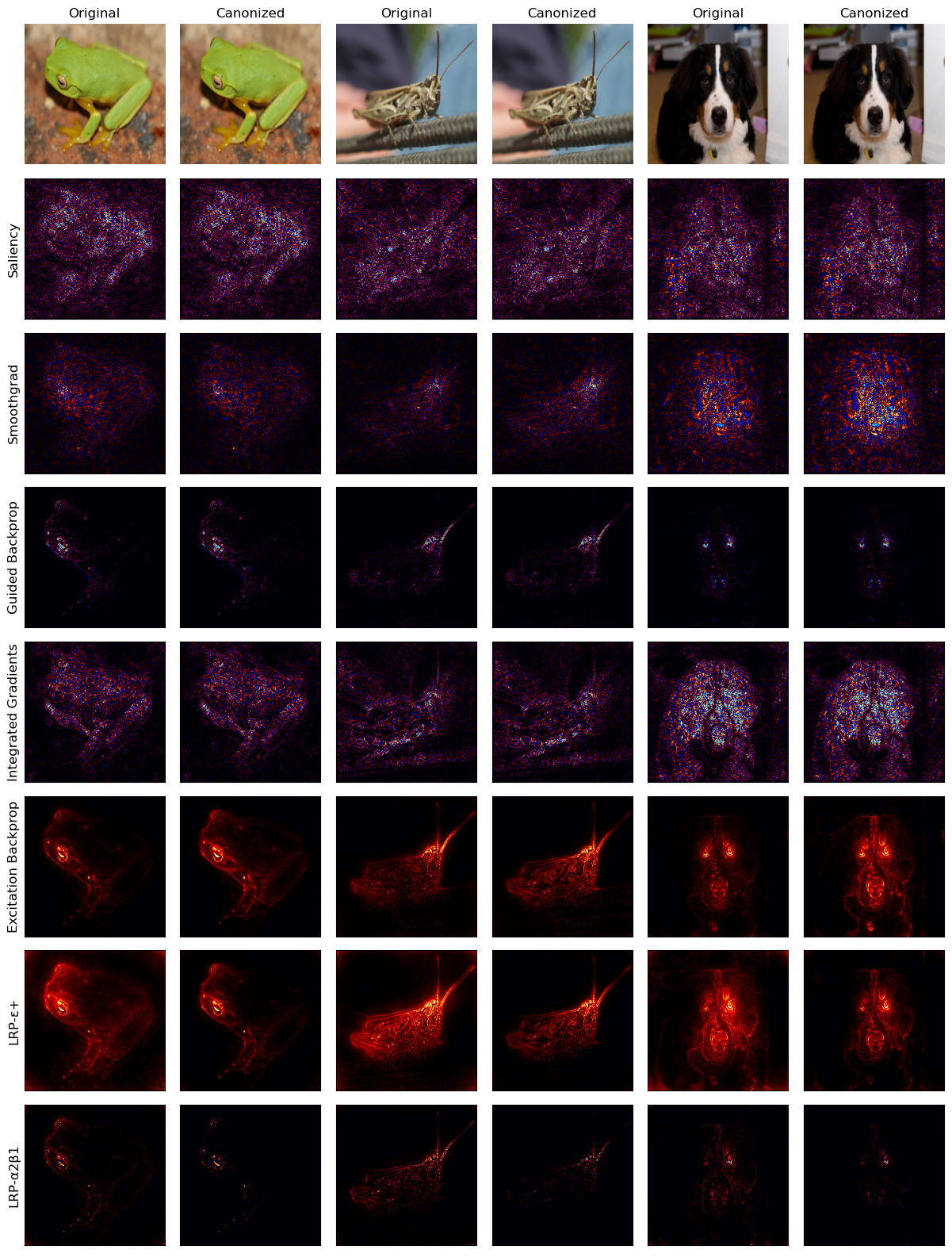
Figure A.2: Attribution heatmaps with different XAI methods for VGG-16 model on ILSVRC2017 dataset.

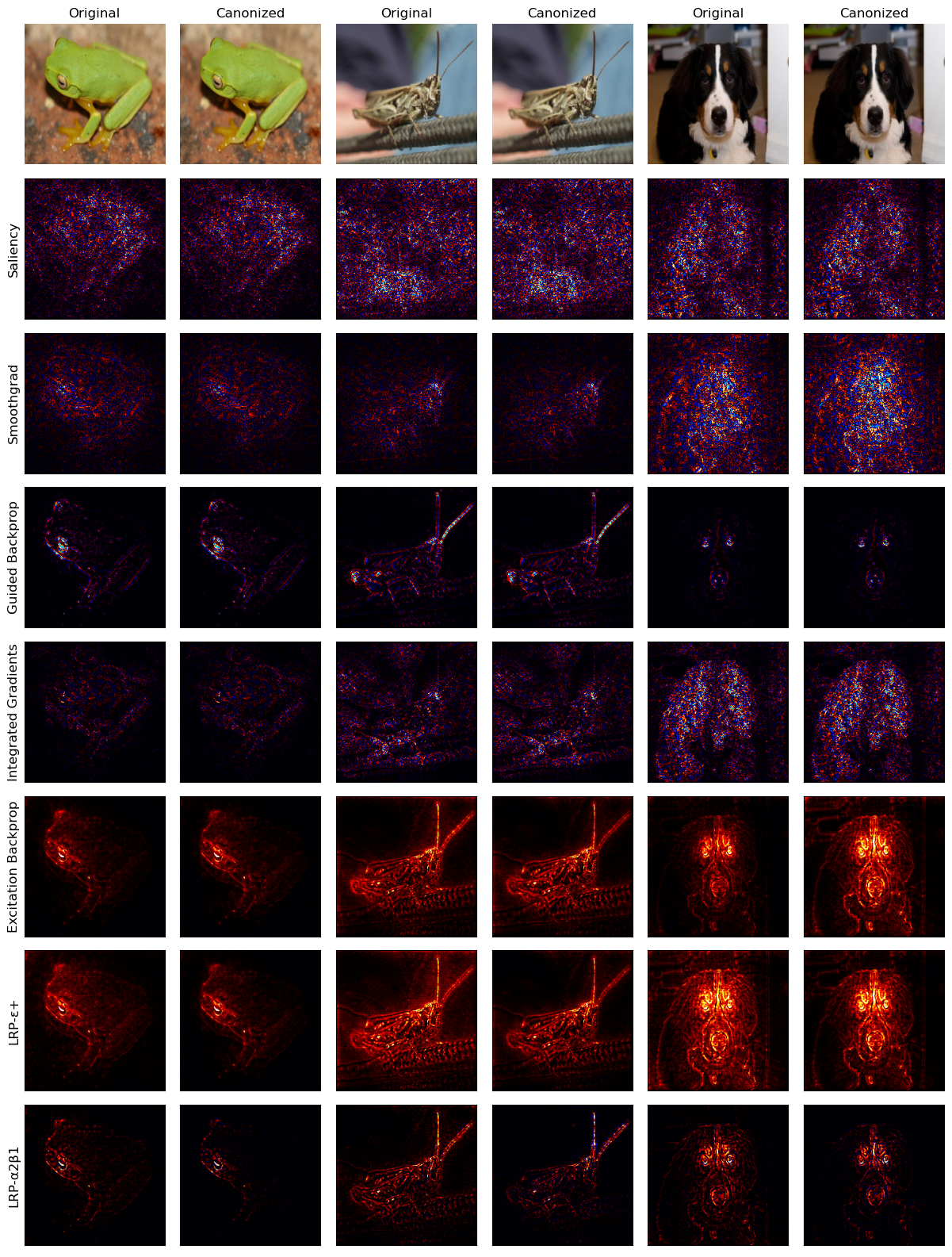
Figure A.3: Attribution heatmaps with different XAI methods for ResNet-18 model on ILSVRC2017 dataset.

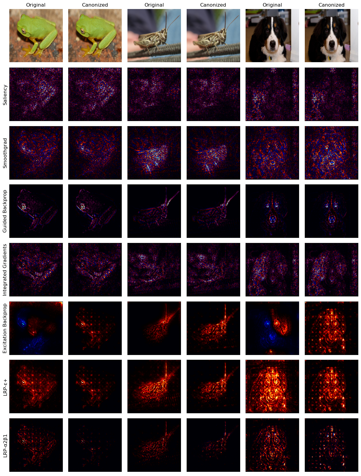
Figure A.4: Attribution heatmaps with different XAI methods for ResNet-50 model on ILSVRC2017 dataset. The checkerboard pattern is due to the downsampling shortcuts in the network. We refer the reader to  [47] for details.

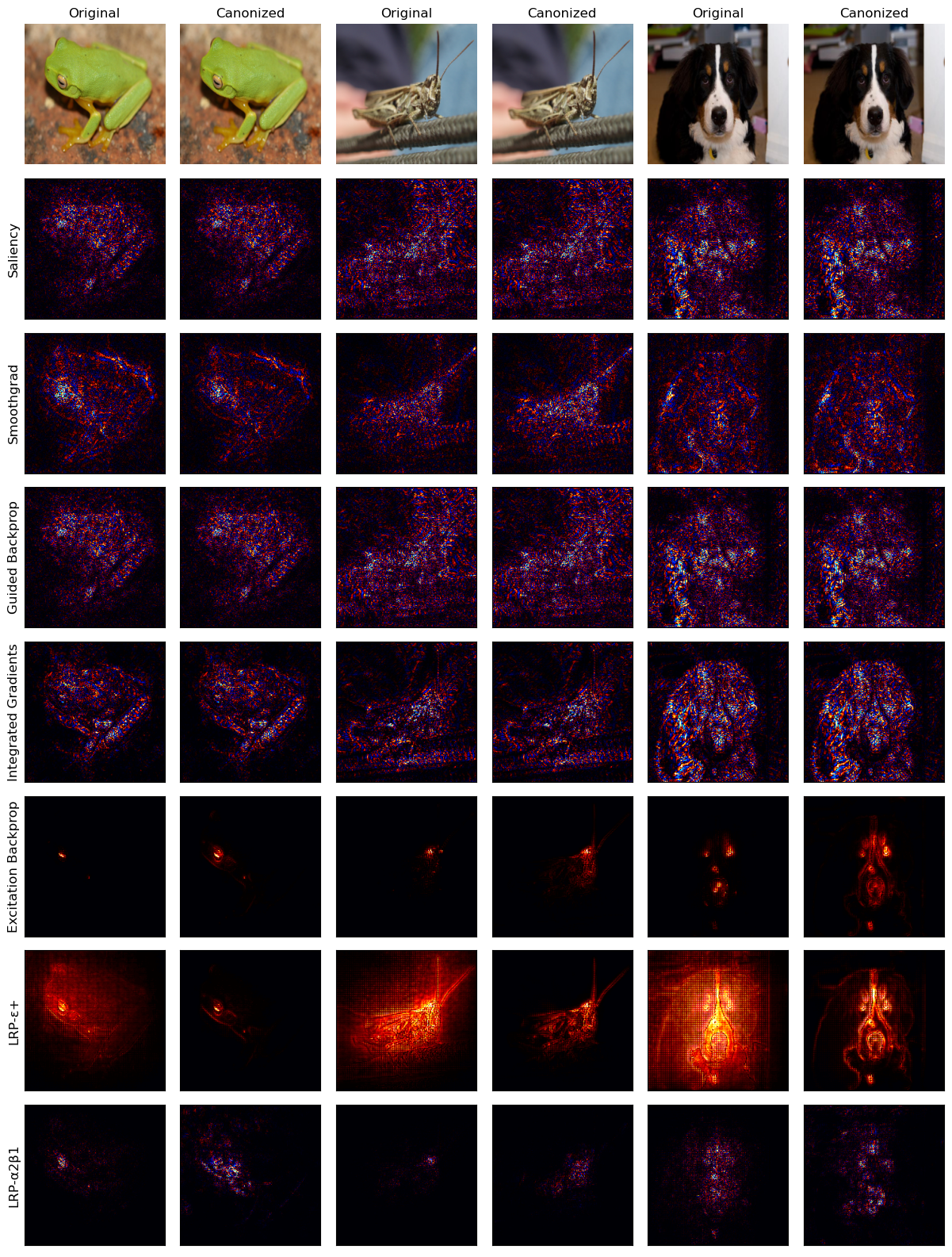
Figure A.5: Attribution heatmaps with different XAI methods for EfficientNet-B0 model on ILSVRC2017 dataset.

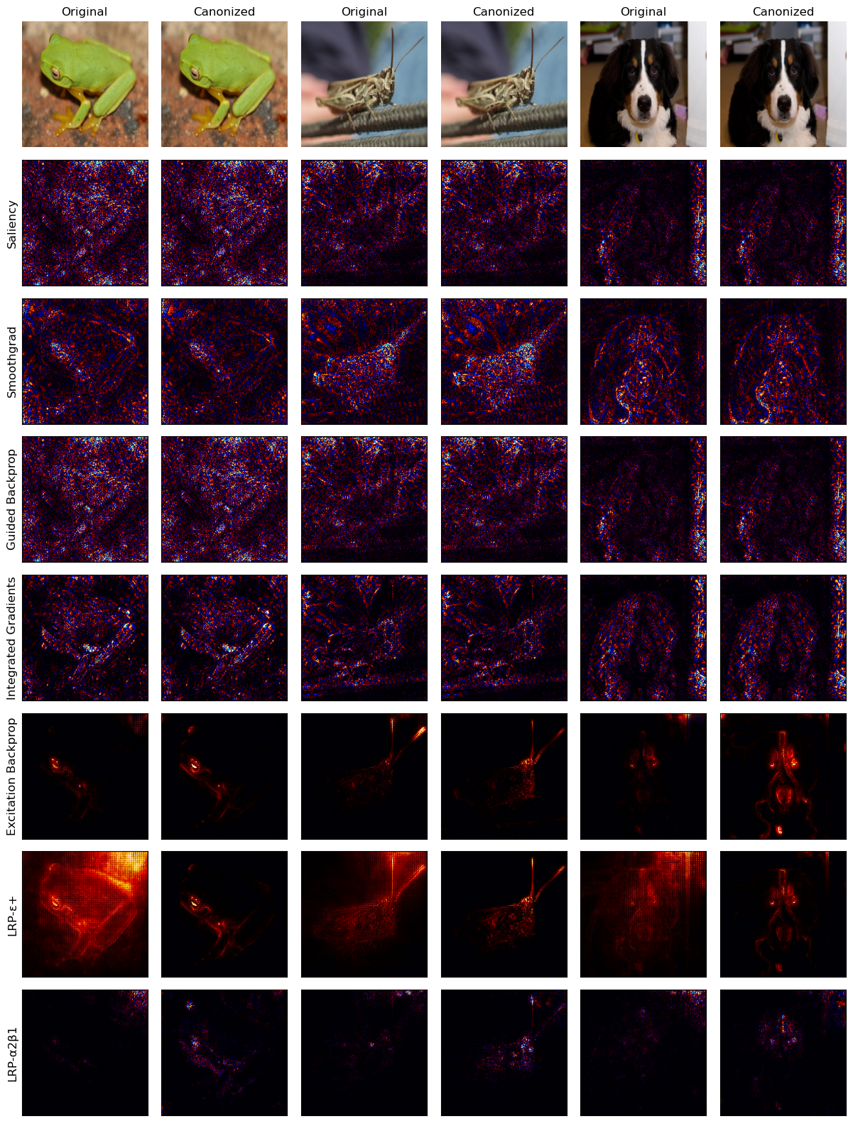
Figure A.6: Attribution heatmaps with different XAI methods for EfficientNet-B4 model on ILSVRC2017 dataset.

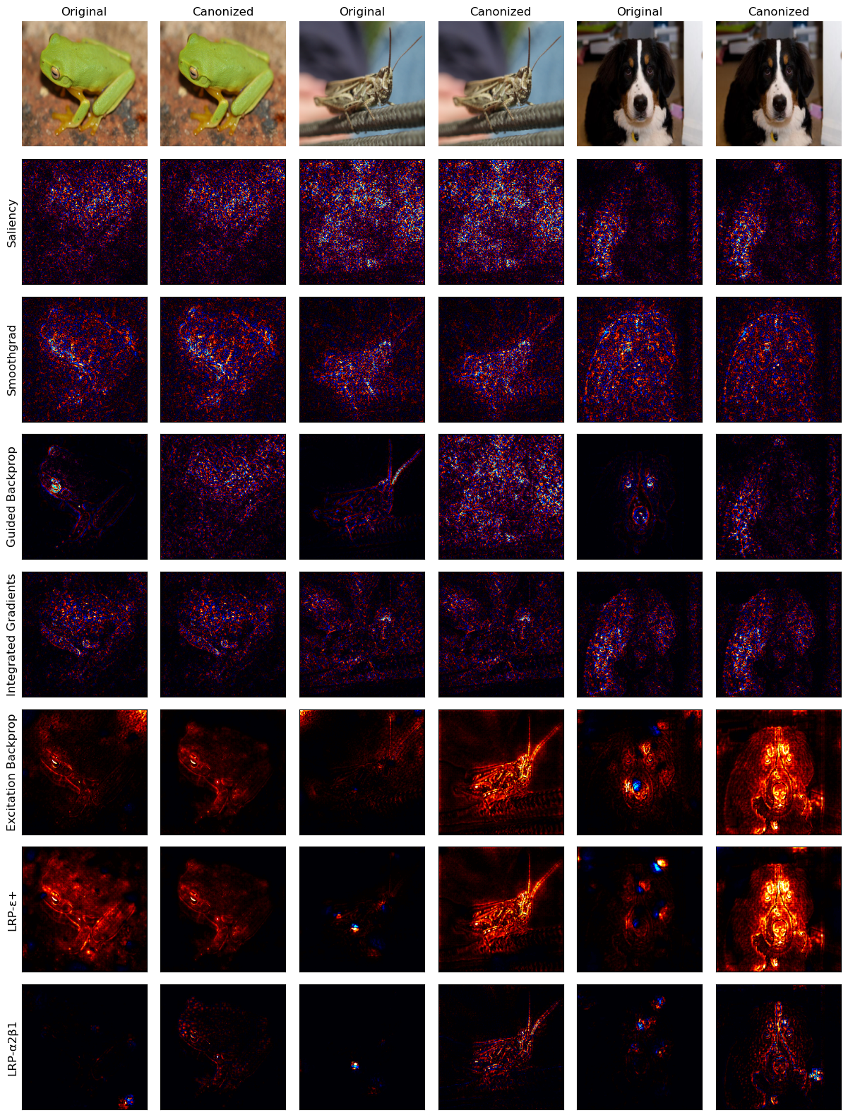
Figure A.7: Attribution heatmaps with different XAI methods for Densenet-121 model on ILSVRC2017 dataset.

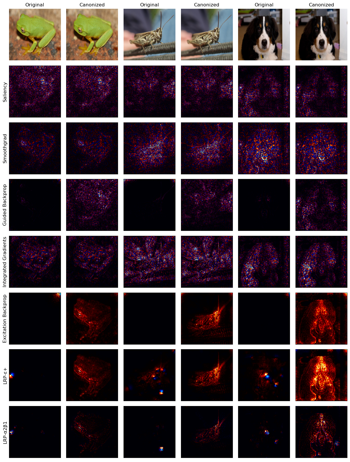
Figure A.8: Attribution heatmaps with different XAI methods for Densenet-161 model on ILSVRC2017 dataset.

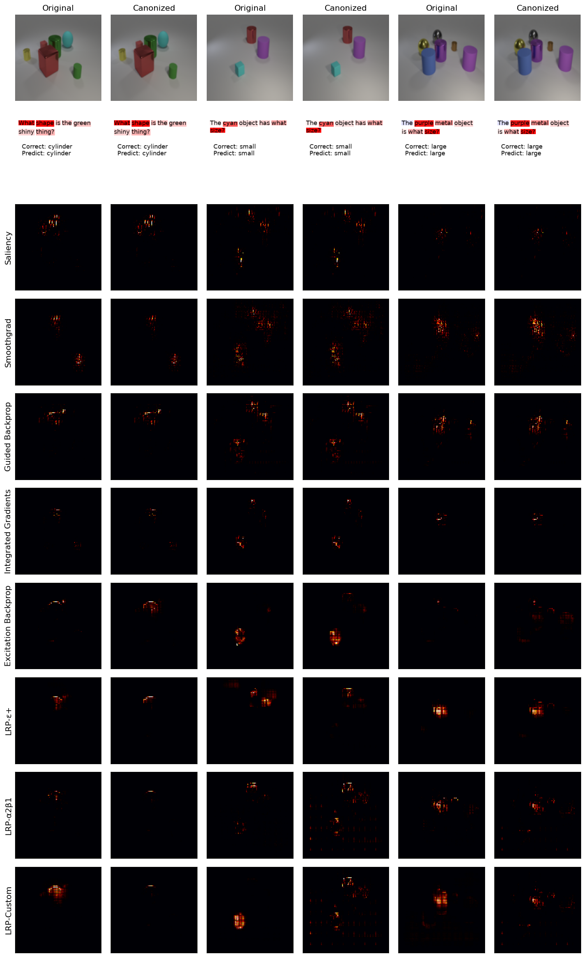
Figure A.9: Attribution heatmaps for Relation Network on CLEVR-XAI dataset using pos-l2-norm-sq pooling.

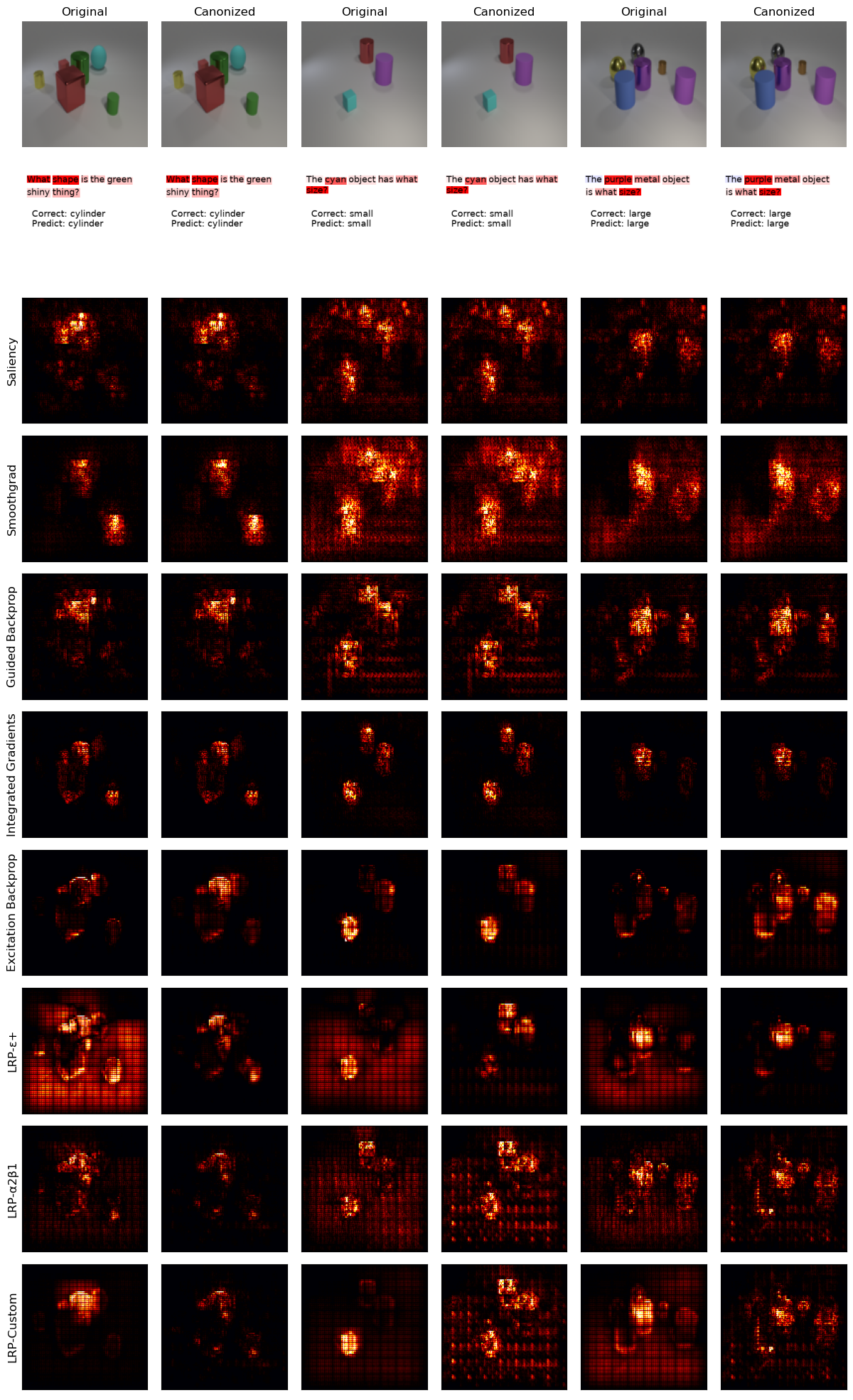
Figure A.10: Attribution heatmaps for Relation Network on CLEVR-XAI dataset using max-norm pooling.

References

- [1] Chirag Agarwal, Eshika Saxena, Satyapriya Krishna, Martin Pawelczyk, Nari Johnson, Isha Puri, Marinka Zitnik, and Himabindu Lakkaraju. Openxai: Towards a transparent evaluation of model explanations. arXiv preprint arXiv:2206.11104, 2022.
- [2] Christopher J. Anders, David Neumann, Wojciech Samek, Klaus-Robert Müller, and Sebastian Lapuschkin. Software for Dataset-wide XAI: From Local Explanations to Global Insights with Zennit, CoRelAy, and ViRelAy. CoRR, abs/2106.13200, 2021.
- [3] Leila Arras, Franziska Horn, Grégoire Montavon, Klaus-Robert Müller, and Wojciech Samek. ” What is relevant in a text document?”: An interpretable machine learning approach. PloS one, 12(8):e0181142, 2017. Publisher: Public Library of Science San Francisco, CA USA.
- [4] Leila Arras, Ahmed Osman, and Wojciech Samek. CLEVR-XAI: a benchmark dataset for the ground truth evaluation of neural network explanations. Information Fusion, 81:14–40, 2022. Publisher: Elsevier.
- [5] Sebastian Bach, Alexander Binder, Grégoire Montavon, Frederick Klauschen, Klaus-Robert Müller, and Wojciech Samek. On pixel-wise explanations for non-linear classifier decisions by layer-wise relevance propagation. PloS one, 10(7):e0130140, 2015. Publisher: Public Library of Science San Francisco, CA USA.
- [6] David Baehrens, Timon Schroeter, Stefan Harmeling, Motoaki Kawanabe, Katja Hansen, and Klaus-Robert Müller. How to explain individual classification decisions. Journal of Machine Learning Research, 11(61):1803–1831, 2010.
- [7] Umang Bhatt, Adrian Weller, and José M. F. Moura. Evaluating and aggregating feature-based model explanations. In Christian Bessiere, editor, Proceedings of the Twenty-Ninth International Joint Conference on Artificial Intelligence, IJCAI-20, pages 3016–3022. International Joint Conferences on Artificial Intelligence Organization, 7 2020. Main track.
- [8] Alexander Binder, Leander Weber, Sebastian Lapuschkin, Grégoire Montavon, Klaus-Robert Müller, and Wojciech Samek. Shortcomings of top-down randomization-based sanity checks for evaluations of deep neural network explanations. arXiv preprint arXiv:2211.12486, 2022.
- [9] Miranda Bogen and Aaron Rieke. Help wanted: An examination of hiring algorithms, equity, and bias. Upturn, December, 7, 2018.
- [10] Titus J Brinker, Achim Hekler, Alexander H Enk, Carola Berking, Sebastian Haferkamp, Axel Hauschild, Michael Weichenthal, Joachim Klode, Dirk Schadendorf, Tim Holland-Letz, and others. Deep neural networks are superior to dermatologists in melanoma image classification. European Journal of Cancer, 119:11–17, 2019. Publisher: Elsevier.
- [11] Prasad Chalasani, Jiefeng Chen, Amrita Roy Chowdhury, Xi Wu, and Somesh Jha. Concise explanations of neural networks using adversarial training. In International Conference on Machine Learning, pages 1383–1391. PMLR, 2020.
- [12] Alexey Dosovitskiy, Lucas Beyer, Alexander Kolesnikov, Dirk Weissenborn, Xiaohua Zhai, Thomas Unterthiner, Mostafa Dehghani, Matthias Minderer, Georg Heigold, Sylvain Gelly, et al. An image is worth 16x16 words: Transformers for image recognition at scale. arxiv 2020. arXiv preprint arXiv:2010.11929, 2010.
- [13] Mark Everingham, Luc Van Gool, Christopher K. I. Williams, John Winn, and Andrew Zisserman. The Pascal Visual Object Classes (VOC) Challenge. International Journal of Computer Vision, 88:303–338, 2010.
- [14] Bryce Goodman and Seth Flaxman. European Union regulations on algorithmic decision-making and a “right to explanation”. AI magazine, 38(3):50–57, 2017.
- [15] Mathilde Guillemot, Catherine Heusele, Rodolphe Korichi, Sylvianne Schnebert, and Liming Chen. Breaking batch normalization for better explainability of deep neural networks through layer-wise relevance propagation. arXiv preprint arXiv:2002.11018, 2020.
- [16] Kaiming He, Xiangyu Zhang, Shaoqing Ren, and Jian Sun. Deep residual learning for image recognition. In Proceedings of the IEEE conference on computer vision and pattern recognition, pages 770–778, 2016.
- [17] Anna Hedström, Leander Weber, Dilyara Bareeva, Franz Motzkus, Wojciech Samek, Sebastian Lapuschkin, and Marina M-C Höhne. Quantus: an explainable ai toolkit for responsible evaluation of neural network explanations. arXiv preprint arXiv:2202.06861, 2022.
- [18] Jie Hu, Li Shen, and Gang Sun. Squeeze-and-excitation networks. In Proceedings of the IEEE conference on computer vision and pattern recognition, pages 7132–7141, 2018.
- [19] Gao Huang, Zhuang Liu, Laurens Van Der Maaten, and Kilian Q Weinberger. Densely connected convolutional networks. In Proceedings of the IEEE conference on computer vision and pattern recognition, pages 4700–4708, 2017.
- [20] Lucas YW Hui and Alexander Binder. Batchnorm decomposition for deep neural network interpretation. In International Work-Conference on Artificial Neural Networks, pages 280–291. Springer, 2019.
- [21] Sergey Ioffe and Christian Szegedy. Batch normalization: Accelerating deep network training by reducing internal covariate shift. In International conference on machine learning, pages 448–456. PMLR, 2015.
- [22] Justin Johnson, Bharath Hariharan, Laurens Van Der Maaten, Li Fei-Fei, C Lawrence Zitnick, and Ross Girshick. Clevr: A diagnostic dataset for compositional language and elementary visual reasoning. In Proceedings of the IEEE conference on computer vision and pattern recognition, pages 2901–2910, 2017.
- [23] Maximilian Kohlbrenner, Alexander Bauer, Shinichi Nakajima, Alexander Binder, Wojciech Samek, and Sebastian Lapuschkin. Towards best practice in explaining neural network decisions with LRP. In 2020 International Joint Conference on Neural Networks (IJCNN), pages 1–7. IEEE, 2020.
- [24] Ilya Loshchilov and Frank Hutter. Sgdr: Stochastic gradient descent with warm restarts, 2016.
- [25] Scott M Lundberg and Su-In Lee. A unified approach to interpreting model predictions. Advances in neural information processing systems, 30, 2017.
- [26] Grégoire Montavon. Gradient-based vs. propagation-based explanations: An axiomatic comparison. In Explainable ai: Interpreting, explaining and visualizing deep learning, pages 253–265. Springer, 2019.
- [27] Grégoire Montavon, Alexander Binder, Sebastian Lapuschkin, Wojciech Samek, and Klaus-Robert Müller. Layer-wise relevance propagation: an overview. Explainable AI: interpreting, explaining and visualizing deep learning, pages 193–209, 2019. Publisher: Springer.
- [28] Grégoire Montavon, Wojciech Samek, and Klaus-Robert Müller. Methods for interpreting and understanding deep neural networks. Digital Signal Processing, 73:1–15, 2018.
- [29] Niels JS Morch, Ulrik Kjems, Lars Kai Hansen, Claus Svarer, Ian Law, Benny Lautrup, Steve Strother, and Kelly Rehm. Visualization of neural networks using saliency maps. In Proceedings of ICNN’95-International Conference on Neural Networks, volume 4, pages 2085–2090. IEEE, 1995.
- [30] Franz Motzkus, Leander Weber, and Sebastian Lapuschkin. Measurably stronger explanation reliability via model canonization. In 2022 IEEE International Conference on Image Processing (ICIP), pages 516–520, 2022.
- [31] Adam Paszke, Sam Gross, Francisco Massa, Adam Lerer, James Bradbury, Gregory Chanan, Trevor Killeen, Zeming Lin, Natalia Gimelshein, Luca Antiga, and others. Pytorch: An imperative style, high-performance deep learning library. Advances in neural information processing systems, 32, 2019.
- [32] Marco Tulio Ribeiro, Sameer Singh, and Carlos Guestrin. ” why should i trust you?” explaining the predictions of any classifier. In Proceedings of the 22nd ACM SIGKDD international conference on knowledge discovery and data mining, pages 1135–1144, 2016.
- [33] Olga Russakovsky, Jia Deng, Hao Su, Jonathan Krause, Sanjeev Satheesh, Sean Ma, Zhiheng Huang, Andrej Karpathy, Aditya Khosla, Michael Bernstein, Alexander C. Berg, and Li Fei-Fei. ImageNet Large Scale Visual Recognition Challenge. International Journal of Computer Vision (IJCV), 115(3):211–252, 2015.
- [34] Wojciech Samek, Alexander Binder, Grégoire Montavon, Sebastian Lapuschkin, and Klaus-Robert Müller. Evaluating the visualization of what a deep neural network has learned. IEEE transactions on neural networks and learning systems, 28(11):2660–2673, 2016. Publisher: IEEE.
- [35] Adam Santoro, David Raposo, David G Barrett, Mateusz Malinowski, Razvan Pascanu, Peter Battaglia, and Timothy Lillicrap. A simple neural network module for relational reasoning. Advances in neural information processing systems, 30, 2017.
- [36] Farah Shahid, Aneela Zameer, and Muhammad Muneeb. Predictions for COVID-19 with deep learning models of LSTM, GRU and Bi-LSTM. Chaos, Solitons & Fractals, 140:110212, 2020. Publisher: Elsevier.
- [37] Avanti Shrikumar, Peyton Greenside, and Anshul Kundaje. Learning important features through propagating activation differences. In International conference on machine learning, pages 3145–3153. PMLR, 2017.
- [38] Avanti Shrikumar, Peyton Greenside, and Anshul Kundaje. Learning important features through propagating activation differences. In International conference on machine learning, pages 3145–3153. PMLR, 2017.
- [39] Karen Simonyan, Andrea Vedaldi, and Andrew Zisserman. Deep inside convolutional networks: Visualising image classification models and saliency maps. arXiv preprint arXiv:1312.6034, 2013.
- [40] Leon Sixt, Maximilian Granz, and Tim Landgraf. When explanations lie: Why many modified bp attributions fail. In International Conference on Machine Learning, pages 9046–9057. PMLR, 2020.
- [41] Daniel Smilkov, Nikhil Thorat, Been Kim, Fernanda Viégas, and Martin Wattenberg. Smoothgrad: removing noise by adding noise. arXiv preprint arXiv:1706.03825, 2017.
- [42] Jost Tobias Springenberg, Alexey Dosovitskiy, Thomas Brox, and Martin Riedmiller. Striving for simplicity: The all convolutional net. arXiv preprint arXiv:1412.6806, 2014.
- [43] Mukund Sundararajan, Ankur Taly, and Qiqi Yan. Axiomatic attribution for deep networks. In International conference on machine learning, pages 3319–3328. PMLR, 2017.
- [44] Christian Szegedy, Wei Liu, Yangqing Jia, Pierre Sermanet, Scott Reed, Dragomir Anguelov, Dumitru Erhan, Vincent Vanhoucke, and Andrew Rabinovich. Going deeper with convolutions. In Proceedings of the IEEE conference on computer vision and pattern recognition, pages 1–9, 2015.
- [45] Mingxing Tan and Quoc Le. Efficientnet: Rethinking model scaling for convolutional neural networks. In International conference on machine learning, pages 6105–6114. PMLR, 2019.
- [46] Gang Wang, Jinxing Hao, Jian Ma, and Hongbing Jiang. A comparative assessment of ensemble learning for credit scoring. Expert systems with applications, 38(1):223–230, 2011.
- [47] Leander Weber, Sebastian Lapuschkin, Alexander Binder, and Wojciech Samek. Beyond explaining: Opportunities and challenges of xai-based model improvement, 2022.
- [48] Chih-Kuan Yeh, Cheng-Yu Hsieh, Arun Suggala, David I Inouye, and Pradeep K Ravikumar. On the (in) fidelity and sensitivity of explanations. Advances in Neural Information Processing Systems, 32, 2019.
- [49] Aleš Završnik. Criminal justice, artificial intelligence systems, and human rights. In ERA Forum, volume 20, pages 567–583. Springer, 2020.
- [50] Jianming Zhang, Sarah Adel Bargal, Zhe Lin, Jonathan Brandt, Xiaohui Shen, and Stan Sclaroff. Top-down neural attention by excitation backprop. International Journal of Computer Vision, 126(10):1084–1102, 2018. Publisher: Springer.