Swarm-Based Gradient Descent Method
for Non-Convex Optimization

Abstract.

We introduce a new Swarm-Based Gradient Descent (SBGD) method for non-convex optimization. The swarm consists of agents, each is identified with a position, $\mathbf{x}$, and mass, $m$. The key to their dynamics is communication: masses are being transferred from agents at high ground to low(-est) ground. At the same time, agents change positions with step size, $h=h(\mathbf{x},m)$, adjusted to their relative mass: heavier agents proceed with small time-steps in the direction of local gradient, while lighter agents take larger time-steps based on a backtracking protocol. Accordingly, the crowd of agents is dynamically divided between ‘heavier’ leaders, expected to approach local minima, and ‘lighter’ explorers. With their large-step protocol, explorers are expected to encounter improved position for the swarm; if they do, then they assume the role of ‘heavy’ swarm leaders and so on. Convergence analysis and numerical simulations in one-, two-, and 20-dimensional benchmarks demonstrate the effectiveness of SBGD as a global optimizer.

1. Introduction

The classical Gradient Descent (GD) methods for optimization, $\mathop{\operatorname*{argmin}}_{\mathbf{x}\in\Omega\subset\mathbb{R}^{d}}F(\mathbf{x})$, explore the ambient space by marching along the directions dictated by local gradients, $\nabla F(\mathbf{x})$. Once the marching direction is determined, the remaining key aspect is a choice of step size.
More often than not, however, GD protocols get trapped in basins of attraction of local minima, and therefore are not suitable for global optimization of non-convex functions.

In this work we introduce a swarm-based gradient descent approach for global optimization.
Communication between agents of the swarm plays a key role in dictating their step size.
Here, the usual ambient space of positions is embedded in $\mathbb{R}^{d}\times[0,1]$: each agent is characterized by its time-dependent position, $\mathbf{x}_{i}(t^{n})\in\Omega\subset\mathbb{R}^{d}$, and its relative weight, $\widetilde{m}_{i}(t^{n})\in[0,1]$.
An interplay between positions and weights proceeds by communicating a dynamic mass transition from high to low, thus our protocol favors agents positioned on ‘lower grounds’.
Looking ahead, the time-stepping protocol is then adjusted according to the distinction between ‘heavy’ agents taking small time steps, and ‘light’ agents taking large(-r) time steps.
While heavy agents take smaller time-steps, expecting their convergence toward a local minimum, light agents proceed with larger time-steps, so that they explore larger regions, away from local basins of attraction; they are expected to improve the global position of the swarm. In the sequel, those light explorers are expected to encounter a ‘better’ minimizing ground.
Then, these light explorers are gradually converted into heavier, global leaders of the swarm.
Here, the dynamic distinction between heavy leaders and light explorers enables a simultaneous approach towards local minimizers, while keep searching for even better global minimizers.

Let us recall other well-known multi-agent optimization algorithms based on ‘wisdom of the crowd’, including particle swarm optimization [13, 7], simulated annealing [15, 27], ant colony optimization [30], genetic algorithm [10] and consensus-based optimization [20, 3, 4, 5].
Our Swarm-Based Gradient descent (SBGD) method is shown to be a most effective optimizer, in particular, when the unknown global minimizer is away from the initial swarm. Visiting larger portions of the ambient space, using explorers based on the communication in swarm dynamics, proved an essential feature for such optimization of remote minimizers. Equally important role is played by the leading agents of the swarm: using the backtracking we prove the sequence of leaders must converge to a minimizer with a quantified rate.

Description of the SBGD method, given in Section 2, highlights the decisive role of communication; indeed, the SBGD can be viewed as alignment dynamics towards minimal heading. A precise time-stepping protocol based on backtracking line search, is outlined in Section 3. Detouring the general paradigm of our swarm-based optimization, we note in Section 4 that our recipe for dynamically adjusting the weights can be extended to more general protocols. In particular, our implementation of SBGD enforces elimination of ‘worst’ agent at each iteration. This ‘survival of the fittest’ approach can be relaxed, increasing the exploring capabilities at the expense of additional computational time. In Section 5 we present convergence and error analysis of SBGD. The time-stepping protocol of backtracking implies that the time sequence of SBGD minimizers has a limit set of one (or more) equi-height minima, and depending on the ‘flatness’ of $F$, expressed in terms of Lojasiewicz bound, there follows convergence rate estimate of the corresponding polynomial order. Finally, in Sections 6, 7 and 8 we present a series of numerical experiments, comparing the SBGD with various GD methods in one-, two- and respectively 20-dimensional problems. These include GD methods with time-stepping protocol based on a fixed time-step, backtracking and momentum-based Adam protocol [14]. These single-agent methods were implemented using $N$ agents with randomly distributed positions. Of course, having $N$ such agents exploring the region of interest, is expected to be “$N$ times better” than their single-agent versions. Still, when compared with our $N$-based swarm method, we found superior performance of SBGD. Specifically, the communication-based approach in SBGD avoids local minima traps, providing better performance when the search for global minimum requires exploration away from the initial ‘blob’ of randomly distributed positions.

2. The Swarm-Based Gradient Descent (SBGD) algorithm

The SBGD dynamics consists of three main ingredients.

• Agents. Each agent is identified by its position, $\mathbf{x}_{i}(t)\in\mathbb{R}^{d}$, and its mass, $m_{i}(t)\in(0,1]$. The total mass is kept constant in time, $\sum_{i}m_{i}(t)=1$.

• Protocol for time step. The position of each agent is dynamically adjusted by taking a time step $h_{i}$ in the gradient direction, $\nabla F(\mathbf{x}_{i}(t))$

  $$\frac{\textnormal{d}}{\textnormal{d}t}\mathbf{x}_{i}(t)=-h_{i}\nabla F(\mathbf{x}_{i}(t)).$$

  The time step, $h_{i}$, depends on the position of the agent at, $\mathbf{x}_{i}(t)$, and on its relative mass, $\widetilde{m}_{i}(t)$,

  $$\widetilde{m}_{i}(t):=\frac{m_{i}(t)}{m_{+}(t)},\quad m_{+}(t)=\max_{i}m_{i}(t).$$

  The precise dynamic protocol for choosing the step size, based on backtracking, is outlined below. A key aspect is choosing $h_{i}$ as a decreasing function of the relative mass, $\widetilde{m}_{i}$: ‘heavier’ agents move slower, while ‘lighter’ agents take larger time steps. An alternative point of view is to interpret the $\widetilde{m}_{i}$’s as the probabilities of agents to identify global minimum: those with mass $m_{i}(t)\ll m_{+}(t)$ take large time steps to explore the region of interest, since their probability of identifying the global minimum at their current position, $\mathbf{x}_{i}(t)$, is low.

• Communication. Let $\displaystyle F_{\textnormal{max}}(t)=\max_{j}F(\mathbf{x}_{j}(t))$ and $\displaystyle F_{\textnormal{min}}(t)=\min_{j}F(\mathbf{x}_{j}(t))$ denote the maximal and respectively, minimal heights of the swarm at time $t$. The mass of each agent, $m_{i}(t)$, is dynamically adjusted according to its relative height, $\displaystyle\eta_{i}(t)$,

  $$\qquad\ \ \left\{\begin{split}\frac{\textnormal{d}}{\textnormal{d}t}m_{i}(t)&=-\phi_{p}(\eta_{i}(t))m_{i}(t),\ i\neq i(t)\\ m_{i}(t)&=1-\sum\limits_{\ j\neq i(t)}\!\!m_{j}(t),\ \ \,i=i(t):=\operatorname*{argmin}_{i}F(x_{i}(t)),\end{split}\right.\quad\eta_{i}(t):=\frac{F(\mathbf{x}_{i}(t))-F_{\textnormal{min}}(t)}{F_{\textnormal{max}}(t)-F_{\textnormal{min}}(t)}.$$

  Thus, each agent ‘sheds’ a fraction of its mass, $\phi_{p}(\eta_{i}(t))\in(0,1]$, which is transferred to the current global minimizer at $\mathbf{x}_{i(t)}$(here we allow to adjust the mass transition, $\phi_{p}(\eta)=\eta^{p}$, using a user choice of a fine-tuning parameter $p>0$, with the default choice $p=1$). As the global minimizer becomes ‘heavier’, it will be ‘cautious’, taking smaller time steps while enabling the other, ‘lighter’ agents, to take larger time steps. As the lighter agents explore the ambient space with larger time steps, it will increase their likelihood to encounter a new neighborhood of a global minimum, which in turn may place one of them as the new heaviest global minimizer and so on. Observe that the larger $p$ is, the more tamed the mass transition of $\phi_{p}(\eta_{i}(t))$.

The discrete time marching of SBGD is realized by agents positioned at $\mathbf{x}^{n+1}_{i}=\mathbf{x}_{i}(t^{n+1})$ with masses $m^{n+1}_{i}=m_{i}(t^{n+1})$ at discrete time steps $t^{n+1}=t^{n}+\Delta t$. We use the simple forward time discretization with time step $\Delta t=1$, acting on all non-empty agents, $m_{i}^{n}>0$,

(2.1) $$\left\{\begin{array}[]{l}\left.\begin{array}[]{lll}\ m_{i}^{n+1}&=m^{n}_{i}-\phi_{p}(\eta^{n}_{i})m^{n}_{i},&i\neq{i_{n}}\\ \\ \ m_{i_{n}}^{n+1}&=\displaystyle m_{i_{n}}^{n}+\sum\limits_{i\neq{i_{n}}}\phi_{p}(\eta^{n}_{i})m_{i}^{n},&\end{array}\right\}\quad{i_{n}}:=\mathop{\operatorname*{argmin}}_{i}F(\mathbf{x}_{i}^{n})\\ \\ \quad\displaystyle m^{n+1}_{+}:=\max_{i}m^{n+1}_{i}\\ \quad\mathbf{x}_{i}^{n+1}=\mathbf{x}_{i}^{n}-h\big{(}\mathbf{x}_{i}^{n},\lambda\psi_{q}(\widetilde{m}^{n+1}_{i})\big{)}\nabla F(\mathbf{x}_{i}^{n}),\quad\displaystyle\widetilde{m}^{n+1}_{i}=\frac{m^{n+1}_{i}}{m^{n+1}_{+}}\par\end{array}\right\}\ \ m_{i}^{n}>0.$$

Initially, the agents are placed at random positions, $\{\mathbf{x}^{0}_{i}\}$ with equi-distributed masses $\{m^{0}_{i}=\nicefrac{{1}}{{N}}\}$. At each iteration, masses of agents are exchanged according to their relative heights, and the positions of agents are updated in the direction of the local gradient, with time step, $h^{n}_{i}=h\big{(}\mathbf{x}_{i}^{n},\lambda\psi_{q}(\widetilde{m}^{n+1}_{i})\big{)}$, depending on these relative mass. Note that the agent with the worst configuration, positioned at $\mathbf{x}_{+}=\operatorname*{argmax}F(\mathbf{x}_{i}^{n})$, is eliminated from the computation; consequently, the size of the swarm decreases, one agent at a time, until it remains with the one heaviest agent. Our choice for the time-stepping protocol, $h\big{(}\mathbf{x},\lambda\psi_{q}(\widetilde{m})\big{)}$, is the backtracking line search outlined in §3.2, which is weighted by the relative masses, $\psi_{q}(\widetilde{m}^{n+1}_{i})$ (again, here we allow fine-tuning the dependence on the relative mass, $\psi_{q}(\widetilde{m})=\widetilde{m}^{q}$, based on a user choice of $q>0$, with the default choice $q=1$). The backtracking enforces a descent property for the SBGD iterations $\mathbf{x}_{i}^{n}$, and the parameter, $\lambda\in(0,1)$, dictates how much the descent property holds in the sense that (3.4) is fulfilled. The communication is designed so that the total mass of the swarm gradually concentrates with the agents most likely to become the global minimizers, that is, the agents which will most likely to reach the global minimum of the region explored so far by the swarm. Such ‘heavy’ agents are assigned with relatively small step sizes, as they are suspected to be close to ’good’ minimizers, hence their subsequent explorations should be sufficiently cautious. On the other hand, the ‘lighter’ agents should not be trapped in basins of attraction of local minimizers, so they proceed with larger step sizes, allowing them to explore a larger regions, during which they may encounter ‘better’ minimizers; then they may be gradually converted from ‘light explorers’ into ‘heavy leaders’ and so on.

We note the flexibility of the SBGD communication protocol, depending on fractional mass transition, $\phi_{p}(\eta^{n}_{i})$, and the mass-dependent step size, $h(\mathbf{x}_{i}^{n},\lambda\psi_{q}(\widetilde{m}^{n+1}_{i}))$. Their detailed construction is outlined in §3. The algorithm (2.1) then forms a family of swarm-based methods, denoted SBGD_pq whenever we want to emphasize its dependence on the parameters $(p,q)$; the ‘vanilla’ version corresponding to $(p,q)=(1,1)$ is denoted simply by SBGD.

2.1. Why communication is important

Consider the particular scenario in which all agents are assigned with the same constant mass, i.e., $m^{n}_{i}\equiv\nicefrac{{1}}{{N}}$ and $\eta_{i}^{n}\equiv 0$, so that $\psi_{q}(\widetilde{m}_{i}^{n})\equiv 1$ yields

(2.2) $$\mathbf{x}_{i}^{n+1}=\mathbf{x}_{i}^{n}-h(\mathbf{x}_{i}^{n},\lambda)\nabla F(\mathbf{x}_{i}^{n}),\qquad i=1,2,\ldots,N.$$

In this case, there is no mass transition and the dynamics is reduced to a crowd of non-communicating agents. In particular, each agent makes its own decision to proceed with variable step size based on the backtracking protocol outlined in section 3.2 below. We refer to this as the backtracking GD, or GD(BT) method. There is also the vanilla version of Gradient Descent, denoted GD(h), which proceeds with a fixed step size $h(\mathbf{x}_{i}^{n},\lambda)\equiv h$. In either case, we have $N$ agents, exploring the region of interest independently of each other. Of course, if there are $N$ such agents exploring the region of interest, the corresponding GD($h$) and GD(BT) method are expected to be “$N$ times better” than their the single-agent versions. However, compared with the swarm of $N$ communicating agents, we find that the SBGD dynamics has a superior global behavior. Specifically, the advantage of communication in SBGD dynamics becomes apparent in exploring larger regions for potential global minimum. This will be borne out in the numerical results presented in sections 6,7 and 8. Here, we demonstrate the benefit of communication with a simple example of an objective function shown in Figure 2.1,

(2.3) $$F(x)=e^{\sin(2x^{2})}+\frac{1}{10}\big{(}x-\frac{\pi}{2}\big{)}^{2}.$$

The function admits multiple local minima, with a unique global minimum ($x^{*}\approx 1.5355$). We compare the performance of SBGD_pq, (2.1) vs. the non-communicating GD(BT) iterations, (2.2), the GD($h$) iterations with a fixed step size $h$, and the Adam method with initial step size $h_{0}$, denoted Adam($h_{0}$), [14]. We report on the results of SBGD₂₁ which seems to perform slightly better than the ‘vanilla’ version SBGD₁₁, and both offer a more robust optimizer than all other non-communicating methods.

Figure 2.1. Plot of the objective function (2.3).

At first, we initialize the positions of agents uniformly in the interval $[-3,3]$. In this case, the global minimum is included in the support of initial data. We implemented 1000 independent simulations and observe the results of SBGD, GD(h), GD(BT) and Adam. Table 2.1 presents the success rates for an increasing number of agents. All methods perform equally well in locating the global minimum, except for Adam(1.1): a large initial step size in Adam method may take it outside the initial region that already contains the global minimum.

The situation is different, however, if we initialize the agents to be uniformly distributed in $[-3,-1]$. The results shown in Table 2.2, indicate that the performance of the non-communicating GD(h), GD(BT) and Adam(0.1) is significantly worse, whereas the SBGD still identifies the global minimum with high success rates. In particular, the GD($h$) and Adam with small time steps are trapped inside an initial basin of attraction, unable to get out of that neighborhood of local minimum. This is also depicted in Figure 2.2 where each local minimum sheds its local basin of attraction for GD(0.8) and Adam(0.1). In particular, the initial data outside $[1,2]$ will necessarily fail to reach the global minimum at $x^{*}\approx 1.5355$. Only when combined with a larger initial step, Adam(1.1) leads to substantial improvement.

This is further clarified when we examine the distribution of $m=1000$ solutions by SBGD vs. GD(BT) in Figure 2.3. Observe that in most of the 1000 experiments, the iterations of GD(BT) are blocked by the relatively flat basin near the origin, and subsequently they end at the local minimizer lying in the interval $[-2,-1]$. In contrast, the SBGD iterations, thanks to the ‘aggressive’ exploration of light agents, are much more likely to avoid getting trapped in the local flat basin of attraction and eventually accumulate enough mass nearby the global minimum.

N	5	10	15	20	30
SBGD11	64.3%	96.5%	99.8%	99.9%	100%
SBGD21	68.2%	97.7%	99.7%	100%	100%
GD(0.8)	75.2%	93.5%	98.7%	100%	100%
GD(BT)	73.6%	96.7%	99.5%	100%	100%
Adam(1.1)	19.6%	35.0%	64.9%	77.1%	89%
Adam(0.1)	58.3%	65.6%	85.8%	95.2%	95.7%

Table 2.1. Success rates of SBGD, GD(h), GD(BT) and Adam methods for global optimization of (2.3), based on $m=1000$ runs with uniformly generated initial data in $[-3,3]$. Backtracking parameters (see algorithm 1), $\lambda=0.2$ and $\gamma=0.9$.

N	5	10	15	20	30
SBGD11	36.5%	83.1%	97.2%	99.5%	100%
SBGD21	42.4%	91.4%	99.0%	99.8%	100%
GD(0.8)	0.0%	0.0%	0.0%	0.0%	0.0%
GD(BT)	1.8%	5.2%	8.5%	12.8%	21.8%
Adam(1.1)	40.2%	47.9%	82.7%	88.7%	93.9%
Adam(0.1)	0.0%	0.0%	0.0%	0.0%	0.0%

Table 2.2. Success rates of SBGD, GD(h), GD(BT) and Adam methods for global optimization of (2.3) based on $m=1000$ runs of uniformly generated initial data in $[-3,-1]$. Backtracking parameters (see algorithm 1), $\lambda=0.2$ and $\gamma=0.9$

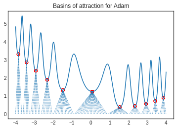
Figure 2.2. Basins of attraction for GD(0.8) and Adam(0.1) method.

The example shows the advantage of communication-based SBGD as an algorithm that is more resilient to the initial guess. Specifically, in complicated applications it may not be realistic to ‘guess’ an initial configuration that encloses the unknown location of the global minimum, and consequently, GD(h), GD(BT) and Adam iterations may be trapped near a local minimizer dictated by ill-conceived initial guesses. In contrast, the final outcome of SBGD is more resilient with respect to the initial configuration, in exploring regions outside the enclosure of initial guesses. More can be found in numerical simulations recorded for one-, two- and 20-dimensional benchmark problems presented, respectively, in sections 6, 7 and 8.

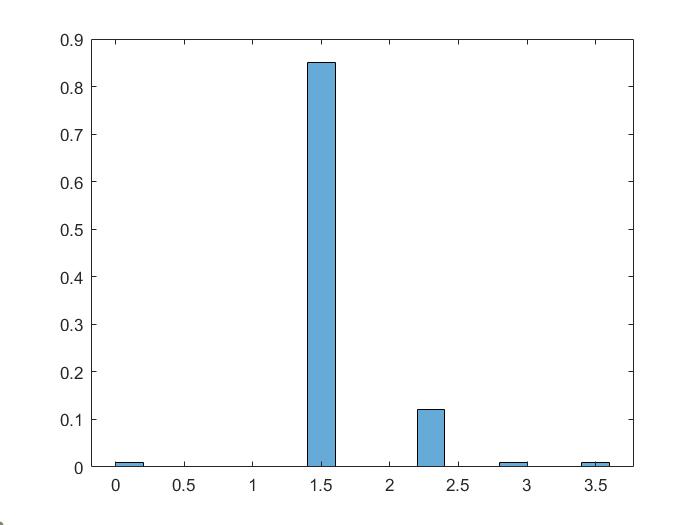
(a) SBGD, $N=10$.

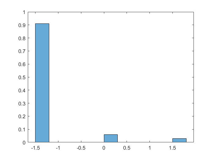
(b) GD(BT) , $N=10$.

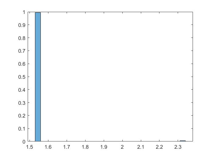
(c) SBGD, $N=20$.

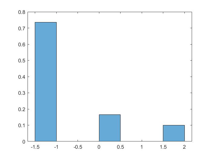
(d) GD(BT) , $N=20$.

(e) SBGD, $N=30$.

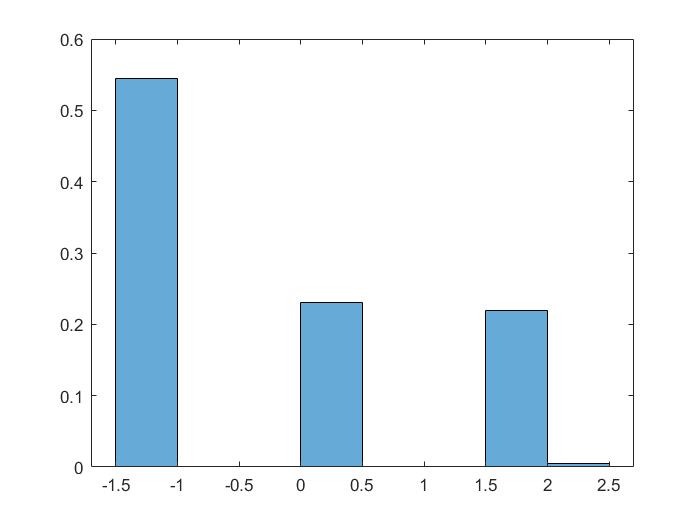
(f) GD(BT) , $N=30$.

Figure 2.3. Histograms of problem (2.3) by $m=200$ experiments. Initial data is generated uniformly in $[-3,-1]$. Global minimum at $x^{*}=1.5355$.

2.2. Alignment towards minimal heading

The dynamic adjustment of masses in SBGD leads to a gradual distinction between ‘leaders’ and ‘explorers’, according to their relative masses. This adjustment of masses (or probabilities), $\widetilde{m}_{i}^{n}$, is dictated by the communication among agents. The SBGD method (2.1) can be also interpreted as a particular case of alignment dynamics, e.g., [25], in which agents steer towards the minimal heading, instead of steering towards the average heading [22]. In the context of alignment for opinion dynamics, for example, the parameter $\widetilde{m}_{i}^{n}$ can be viewed as fraction of the population supporting ‘opinion’ $\mathbf{x}_{i}^{n}$.
This is reminiscent of the Consensus-Based Optimization (CBO) method, first proposed in [20] and further modified and analyzed in [3, 4, 8, 9]; see recent survey [26]. The CBO method lets a swarm of agents evolve their positions, $\{\mathbf{x}^{j}_{t}\}$, by a stochastic motion in search of a global minimizer,

(2.4) $$\textnormal{d}\mathbf{x}^{j}_{t}=-\lambda(\mathbf{x}^{j}_{t}-{\mathbf{m}}^{N}_{t}){\textnormal{d}}t+\sigma(\mathbf{x}^{j}_{t}-{\mathbf{m}}^{N}_{t}){\textnormal{d}}{\bf W}^{j}_{t},\quad\lambda,\sigma>0$$

Agents are driven by two types of motions: the drift towards an exponentially weighted average, ${\mathbf{m}}^{N}_{t}:=\big{(}\sum_{j=1}^{N}(F_{e})^{j}_{t}\big{)}^{-1}\sum_{j=1}^{N}\mathbf{x}^{j}_{t}(F_{e})^{j}_{t},\ (F_{e})^{j}_{t}:=exp(-\alpha F(\mathbf{x}^{j}_{t}))$, and the stochastic diffusion, ${\textnormal{d}}{\bf W}^{j}_{t}$ (implemented by independent Brownian motion different components, $\sum^{d}_{k=1}(\mathbf{x}^{j}_{t}-{\mathbf{m}}^{N}_{t})_{k}{\textnormal{d}}W^{j,k}_{t}\vec{e}_{k}$). By the Laplace principle, [2], the exponentially weighted average, ${\mathbf{m}}^{N}_{t}$, concentrates most of its weight with agents of minimal height (or smallest loss). Thus, the drift in (2.4) aligns towards those agents with minimal heading, while the stochastic diffusion is responsible for enhancing the other agents to explore a larger portion of the domain. This should be compared with the deterministic SBGD method, where explorers are driven by communication with lightweight agents.
Unlike gradient-based methods, the CBO has the advantage of avoiding computation of gradients, which are replaced here by a drift towards the $\alpha$-weighted average. In actual computation, however, in particular in high-dimensional problems, the CBO method is sensitive to the application of the $\alpha$-weighted Laplace principle, requiring $\alpha\gg 1$, which is likely to significantly damage the quality of the solution. It is also sensitive to the choice of parameters $\lambda$ and $\sigma$, [4].

3. Implementation of the SBGD_pq algorithm

The success of the SBGD_pq method relies heavily on two main procedures: (i) a properly defined communication protocol which dictates mass transition factors, $\{\phi_{p}(\eta^{n}_{i})\}$; and (ii) an effective strategy for taking step size, $h\big{(}\mathbf{x}_{i}^{n},\psi_{q}(\widetilde{m}^{n+1}_{i})\big{)}$, which is adjusted to the position and the relative mass of a given agent. In this section, we discuss the details of these procedures, which are summarized in corresponding pseudo-codes.

3.1. Communications and mass transition

Let $\displaystyle{i_{n}}=\operatorname*{argmin}_{i}F(\mathbf{x}^{n}_{i})$ denote the global minimizer at iteration number $n$ or time level $t^{n}$. All other agents will shed part (or all) of their mass, $\phi_{p}(\eta^{n}_{i})m^{n}_{i},\ i\neq{i_{n}}$, which will be transitioned to the mass of the global minimizer $\displaystyle m^{n}_{i_{n}}\mapsto m^{n}_{i_{n}}+\sum_{i\neq{i_{n}}}\phi_{p}(\eta^{n}_{i})m^{n}_{i}$. The fraction of mass loss, $\eta^{n}_{i}$ is determined by the relative height

(3.1) $$\eta^{n}_{i}:=\frac{F(\mathbf{x}_{i}^{n})-F^{n}_{\textnormal{min}}}{F^{n}_{\textnormal{max}}-F^{n}_{\textnormal{min}}+\epsilon},$$

where $\displaystyle F^{n}_{\textnormal{min}}=\min_{j}F(\mathbf{x}^{n}_{j})$ and $\displaystyle F^{n}_{\textnormal{max}}=\max_{j}F(\mathbf{x}^{n}_{j})$ are the current global extremes. In this fashion, the ‘higher’ the agent is, the more mass it will lose, and indeed, the highest agent in each iteration will be eliminated. The function $\phi$ is user-dependent; for example $\phi_{p}(\eta)=\eta^{p},\ p>0$ enables adjusting the amount of mass transition, with mass transition tamed as $p\uparrow\infty$. This usage of a relative height keeps a minimal amount of global communication necessary to calibrate each agent relative to the current extremes of the crowd, while being invariant under the transition and dilation of the target function. Therefore, the computation of the relative height is more stable.

3.2. Backtracking – a protocol for time stepping

Consider the vanilla Gradient Descent (GD) iteration

$$\mathbf{x}^{n+1}=\mathbf{x}^{n}-h\nabla F(\mathbf{x}^{n}).$$

The new position, $\mathbf{x}^{n+1}=\mathbf{x}^{n+1}(h)$, is viewed as a function of the step size, $h$. A proper strategy for choosing the step size is now the key for the success of GD iterations. We recall the classical backtracking line search, [19, §3], which is a computational realization of the well-known Wolfe conditions [29, 1] for inexact line searches. The idea is to secure an acceptable step length, $h$, that enforces a sufficient amount of height reduction (or loss) in the target function

(3.2) $$F(\mathbf{x}^{n+1}(h))\leqslant F(\mathbf{x}^{n})-\lambda h|\nabla F(\mathbf{x}^{n})|^{2},\quad\lambda\in(0,1).$$

Of course, since $F((\mathbf{x}^{n+1}(h))=F(\mathbf{x}_{i}^{n})-h|\nabla F(\mathbf{x}^{n})|^{2}+\textnormal{\{higher order terms\}}$, then (3.2) holds for any fixed $0<\lambda<1$, provided the time step is small enough, $h\ll 1$. The purpose is to secure (3.2) for large enough $h$, so that we maximize the size of descent, $\lambda h|\nabla F(\mathbf{x}^{n})|^{2}$. To this end, one employs a dynamic adjustment, starting with a relatively large $h$ (for which one expects $\displaystyle F\big{(}\mathbf{x}^{n}-h\nabla F(\mathbf{x}^{n})\big{)}>F(\mathbf{x}^{n})-\lambda h|\nabla F(\mathbf{x}^{n})|^{2}$) and then successively shrink the step size $h$ until (3.2) is observed. At this stage, we have a final step size, $h=h(\mathbf{x}^{n},\lambda)$, which secure (3.2)

$$F(\mathbf{x}^{n+1}(h))\leqslant F(\mathbf{x}^{n})-\lambda h(\mathbf{x}^{n},\lambda)|\nabla F(\mathbf{x}^{n})|^{2}.$$

Thus, the protocol for step size hinges on the choice of the parameter $\lambda$ which dictates the amount of descent property (3.2). One expects that as the iterations approach the (potentially) global minimum their descent property is ‘tamed’ with a larger $\lambda$, yet they should be able to avoid getting trapped in local basins of attraction by allowing smaller $\lambda\ll 1$. This is exactly where we take advantage of our swarm-based approach: as a compromise between these two conflicting requirements, we offer to use the relative mass of different agents, $\widetilde{m}^{n+1}_{i}$, as an indicator which distinguishes between the ‘heavier’ agents who are potentially close to the global minimizer, and the ‘lighter’ agents which are allowed to take large(r) time steps. We therefore adjust the descent parameter $\lambda$ to each SBGD_pq agent positioned at $\mathbf{x}_{i}^{n}$, according to its relative mass $\widetilde{m}^{n+1}_{i}$

(3.3) $$h^{n}_{i}=h\big{(}\mathbf{x}_{i}^{n},\lambda\psi_{q}(\widetilde{m}^{n+1}_{i})\big{)}\qquad\widetilde{m}^{n+1}_{i}:=\frac{m^{n+1}_{i}}{m{}^{n+1}_{+}},\quad m{}^{n+1}_{+}:=\max_{i}m^{n+1}_{i},\ \ 0<\lambda<1.$$

The parameter $q>0$ tunes the role of the relative mass $\widetilde{m}^{n+1}_{i}$: as $q$ increases then $\psi_{q}(\widetilde{m}^{n+1}_{i})$ decreases, and backtracking allows intermediate agents to take larger time steps. The pseudo-code for computing the SBGD_pq steps based on backtracking line search is given in Algorithm 1. The results reported in §7.3 below show that although fine-tuning the parameter, $q$, can lead to improved results, it has a limited effect on the overall performance of SBGD_pq iterations.

Algorithm 1 Backtracking Line Search

Set the descent parameter, $\lambda\in(0,1)$, and shrinkage parameter, $\gamma\in(0,1)$

Set $\psi_{q}$ with $q>0$

Set the relative mass $\displaystyle\widetilde{m}^{n+1}_{i}=\frac{m^{n+1}_{i}}{m^{n+1}_{+}}$

Initialize the step size $h=h_{0}$.

while $F\big{(}\mathbf{x}_{i}^{n}-h\nabla F(\mathbf{x}_{i}^{n})\big{)}>F(\mathbf{x}_{i}^{n})-\lambda\psi_{q}(\widetilde{m}^{n+1}_{i})h|\nabla F(\mathbf{x}_{i}^{n})|^{2}$ do

     $h\leftarrow\gamma h$.

end while Set $h\big{(}\mathbf{x}_{i}^{n},\lambda\psi_{q}(\widetilde{m}^{n+1}_{i})\big{)}\leftarrow h$

Observe that the successive shrinking of step size in backtracking involves a shrinking factor $\gamma\in(0,1)$: a small $\gamma$ corresponds to a ‘crude’ line search while $\gamma\sim 1$, corresponds to a more refined search. Again, although fine-tuning the shrinkage parameter $\gamma$ may lead to improved results, it does not seem to have a substantial effect on the overall performance of SBGD_pq.

The final output of algorithm 1 yields, for each agent, an adjusted step size, $h^{n}_{i}=h\big{(}\mathbf{x}_{i}^{n},\lambda\psi_{q}(\widetilde{m}^{n+1}_{i})\big{)}$, which secures the descent property (3.2) with $\lambda\psi_{q}(\widetilde{m}^{n+1}_{i})$ substituted for $\lambda$,

(3.4) $$F(\mathbf{x}^{n+1}_{i})\leqslant F(\mathbf{x}_{i}^{n})-\lambda\psi_{q}(\widetilde{m}^{n+1}_{i})h^{n}_{i}|\nabla F(\mathbf{x}^{n})|^{2},\qquad\quad\mathbf{x}^{n+1}_{i}=\mathbf{x}_{i}^{n}-h^{n}_{i}\nabla F(\mathbf{x}_{i}^{n}).$$

Moreover, as we shall see in Lemma 5.1 below, the step sizes, $h^{n}_{i}$, admit a lower bound in terms of the corresponding relative masses of the different agents. The scaling of the step size using relative masses encodes the communication of different agents, which is the key to the success of the SBGD_pq algorithm. Roughly speaking, we can distinguish between two types of agents. The SBGD_pq iterations are led by the heavier agents, $m^{n+1}_{i}\approx m{{}^{n+1}_{+}}$, which tend to recover a maximal local descent rate of order $\lambda$, (3.2). On the other hand, there are the lighter agents where $\displaystyle m^{n+1}_{i}\ll m{{}^{n+1}_{+}}$, which are less driven by the steepness of their decent, and are therefore better equipped as explorers of large areal search for the global minimizer. In this way, the mass-dependent adjustment of step size captures both the descent property of the target function while allowing the lighter explorers to pull away from local minimizers.

3.3. SBGD_pq pseudocode

The pseudocode of the SBGD_pq method is given in Algorithm 2. The initial setup consists of $N$ randomly distributed agents $\mathbf{x}^{0}_{1},\cdots,\mathbf{x}_{N}^{0}$, associated with masses $m_{1}^{0},\cdots,m_{N}^{0}$. At the beginning, all agents are assigned equal masses, $\displaystyle m_{j}^{0}=\nicefrac{{1}}{{N}}$, $j=1,\ldots,N$. At each iteration step, the agent $\mathbf{x}_{i_{n}}=\operatorname*{argmin}_{\mathbf{x}_{i}^{n}}F(\mathbf{x}_{i}^{n})$ attains the minimal value, while the other agents transfer part of their masses to the current optimal minimizer $\mathbf{x}_{i_{n}}$. Then all the agents are updated with the gradient descent method using the step lengths obtained with (3.3).

To further improve efficiency, we use three tolerance factors:
$\cdot$ If the mass of an agent is lower than a minimal threshold $tolm$, then this agent will be eliminated and its remaining mass will be transferred to the optimal agent at $\mathbf{x}_{i_{n}}$.
$\cdot$ “Sticking particles”. Agents that are sufficiently close to each other below a threshold $tolmerge$, are merged into a new agent, and their masses are combined into the newly generated agent.
$\cdot$ The iterations stop when the minimizer’s descent in two consecutive iterations is below a minimal threshold $tolres$.

Unless otherwise specified, all simulations reported in this paper employ the same thresholds

(3.5) $$tolm=10^{-4},\quad tolmerge=10^{-3},\quad tolres=10^{-4}.$$

The optimal choices of these thresholds are experimental. With smaller thresholds, $tolm$ and $tolmerge$, the SBGD algorithm will explore a larger part of the ambient space ending with a better solution, at the expense of reduced efficiency. A balance between the quality of the solution and the computational cost should be explored.

Algorithm 2 Swarm-Based Gradient Descent

Set three tolerance parameters, $tolm$, $tolmerge$ and $tolres$

Set the adjustment parameters $p,q>0$

Initialization:

  Set $N$ — the number of agents

  Set initial positions $\mathbf{x}_{1}^{0},\cdots,\mathbf{x}_{N}^{0}$ randomly generated under initial distribution $\rho_{0}$

  Set initial mass $\displaystyle m^{0}_{1}=\cdots=m^{0}_{N}=\nicefrac{{1}}{{N}}$

  Set the optimal agent, $\displaystyle i_{0}=\operatorname*{argmin}_{i}F(\mathbf{x}^{0}_{i})$

for $n=0,1,2,\cdots$ do

     Set $\displaystyle F{{}^{n}_{-}}=F(\mathbf{x}^{n}_{i_{n}})$, $\displaystyle F{{}^{n}_{+}}=\max_{i}F(\mathbf{x}_{i}^{n})$

     for $i=1,\cdots,N$ and $i\neq{i_{n}}$ do    % Mass transitions

         if $\displaystyle m_{i}^{n}<\nicefrac{{1}}{{N}}*tolm$ then

              set $m_{i}^{n+1}=0$

              reduce the $\#$ of active agents: $N\leftarrow N-1$

         else $\displaystyle m_{i}^{n+1}=m^{n}_{i}-\phi_{p}(\eta^{n}_{i})m^{n}_{i}$ where $\displaystyle\eta^{n}_{i}=\frac{F(\mathbf{x}_{i}^{n})-F^{n}_{\textnormal{min}}}{F^{n}_{\textnormal{max}}-F^{n}_{\textnormal{min}}}$.

         end if

     end for

     $\displaystyle m_{i_{n}}^{n+1}=m_{i_{n}}^{n}+\sum_{i\neq{i_{n}}}\phi_{p}(\eta^{n}_{i})m^{n}_{i}$             % The mass of the overall crowd is conserved

     Compute $\displaystyle m_{+}=\max_{i}m^{n+1}_{i}$

     for $i=1,\cdots,N$ do                  % Gradient descent

         Compute relative masses $\displaystyle\widetilde{m}^{n+1}_{i}=\frac{m^{n+1}_{i}}{m_{+}}$

         Compute the step size $h=h\big{(}\mathbf{x}_{i}^{n},\lambda\psi_{q}(\widetilde{m}^{n+1}_{i})\big{)}$ according to algorithm 1.

         March: $\displaystyle\mathbf{x}_{i}^{n+1}=\mathbf{x}_{i}^{n}-h\nabla F(\mathbf{x}_{i}^{n})$.

     end for

     Merge the agents if their distance $<tolmerge$.

     Set the new optimal agent $i_{n+1}$ = $\displaystyle\operatorname*{argmin}_{i}F(\mathbf{x}^{n+1}_{i})$.

     Compute the residual $\displaystyle res=|\mathbf{x}^{n+1}_{i_{n+1}}-\mathbf{x}^{n}_{i_{n}}|_{2}$

     if $res<tolres$ then

         $\mathbf{x}_{SOL}\leftarrow\mathbf{x}^{n+1}_{i_{n+1}}$

         break

     end if

end for

4. A general outlook

We are aware that there are many possible extensions that can be worked out in connection with the SBGD algorithm, leading to a large class of swarm-based optimizers (SBO) with better communication protocols. We mention three of them.

$\cdot$ General gradient descent directions

Our SBGD approach can be used with a more general set of gradient descent directions, ${\mathbf{p}}^{n}_{i}$

$$\mathbf{x}^{n+1}_{i}=\mathbf{x}_{i}^{n}+h\big{(}\mathbf{x}_{i}^{n},\lambda\psi_{q}(\widetilde{m}^{n+1}_{i})\big{)}{\mathbf{p}}^{n}_{i},\qquad\langle{\mathbf{p}}^{n}_{i},\nabla F(\mathbf{x}_{i}^{n})\rangle<0.$$

The convergence results in §5, with appropriate adjustments, remain valid. Moreover, the variety in choice of directions, other than local gradients, may offer a better ‘covering’ of the ambient space $\Omega\subset{\mathbb{R}}^{d}$.

$\cdot$ Swarm-based optimization — a general paradigm

The general paradigm for our swarm-based optimization is realized by embedding the $d$-dimensional ambient space in $(\mathbf{x},\widetilde{m})\in{\mathbb{R}}^{d}\times[0,1]$; here $\widetilde{m}$ is an additional parameter space of masses/weights (or probabilities, or ‘fractional population’, …) which serves as a communication platform for the crowd of agents positioned at $\{\mathbf{x}_{i}\}\in{\mathbb{R}}^{d}$. In this context, one can combine such communication-based swarm iterations with any single agent time-marching protocol. As examples we refer to the recent adaptive GD method [17] and the references therein. In the present work we use the time-marching protocol of gradient-descent, based on backtracking search. Other time marching protocols can be used.

$\cdot$ Survival of the fittest

The communication in SBGD is designed so that in each iteration, the ‘worst’ agent, positioned at $\displaystyle\mathbf{x}_{{i_{+}}}:=\operatorname*{argmax}_{\mathbf{x}_{i}}F(\mathbf{x}_{i}^{n})$, is eliminated, as it loses all of its mass ($\eta_{i_{+}}^{n}=1$). This policy of ‘survival of the fittest’ implies that the number of $N$ initial active agents decreases in each iteration until the SBGD remains with only a single, ‘heaviest’ agent, which proceeds by the GD(BT) protocol. In particular, this policy implies that for small swarms, say $N\sim 10$, the performance of SBGD iterations is expected to be similar or only slightly better than GD(BT) iterations, as borne out in the numerical simulations reported in sections 7 and 8. Alternatively, one can design a less restrictive evolutionary policy that will allow ‘worst’ agents below a certain threshold to survive. This will evolve a larger set of explorers for longer times, with a greater chance of exploring new and better minima unseen before. Our numerical experiments show that a balanced policy for the ‘fittest’ can indeed have a substantial effect on the final result, at the expense of increased computational time.

5. Convergence and error analysis

The study of convergence and error estimates for the SBGD method requires to quantify the behavior of $F$. Here we emphasize that the required smoothness properties of $F$ are only sought in the region explored by the SBGD iterations. We assume that there exists a bounded region, $\Omega\ni\mathbf{x}_{i}^{n}$ for all agents. Since the SBGD allows light agents to explore the ambient space with large step size (starting with $h_{0}$), we do not have apriori bound on $\Omega$; in particular, the footprint of the SBGD crowd $\textnormal{conv}_{i}\{\mathbf{x}_{i}^{n}\}$ may expand well beyond its initial convex hull $\textnormal{conv}_{i}\{\mathbf{x}^{0}_{i}\}$.
We consider the class of loss functions, $F\in C^{2}(\Omega)$, with Lipschitz bound

(5.1) $$|\nabla F(\mathbf{x})-\nabla F(\mathbf{y})|\leqslant L|\mathbf{x}-\mathbf{y}|,\quad\forall\mathbf{x},\mathbf{y}\in\Omega.$$

We begin by recalling the lower bound on the step size, secured by the backtracking line search in algorithm 1.

Lemma 5.1.

Consider the SBGD_pq iterations (2.1), with step size $h^{n}_{i}=h\big{(}\mathbf{x}_{i}^{n},\lambda\psi_{q}(\widetilde{m}^{n+1}_{i})\big{)}$ determined by backtracking line search in algorithm 1 with shrinkage factor $\gamma\in(0,1)$. Then we have a lower bound on the step length

(5.2) $$h^{n}_{i}\geqslant\frac{2\gamma}{L}\big{(}1-\lambda\psi_{q}(\widetilde{m}^{n+1}_{i})\big{)}.$$

Proof. By the Lipschitz continuity of $\nabla F$,

$$\begin{split}F\big{(}\mathbf{x}_{i}^{n}-h^{n}_{i}\nabla F(\mathbf{x}_{i}^{n})\big{)}&\leqslant F(\mathbf{x}^{n})-h^{n}_{i}|\nabla F(\mathbf{x}_{i}^{n})|^{2}+\frac{L}{2}(h^{n}_{i})^{2}|\nabla F(\mathbf{x}_{i}^{n})|^{2}\\ &=F(\mathbf{x}_{i}^{n})-\Big{(}1-\frac{L}{2}h^{n}_{i}\Big{)}h^{n}_{i}|\nabla F(\mathbf{x}_{i}^{n})|^{2},\end{split}$$

and hence, if $h^{n}_{i}$ is small enough

$$h^{n}_{i}\leqslant\frac{2}{L}\big{(}1-\lambda\psi_{q}(\widetilde{m}^{n+1}_{i})\big{)}\ \ \leadsto\ \ F(\mathbf{x}_{i}^{n}-h^{n}_{i}\nabla F(\mathbf{x}_{i}^{n}))\leqslant F(\mathbf{x}_{i}^{n})-\lambda\psi_{q}(\widetilde{m}^{n+1}_{i})h^{n}_{i}|\nabla F(\mathbf{x}_{i}^{n})|^{2}.$$

The backtracking line search iterations tell us that the inequality on the right holds for $h^{n}_{i}$ but not for $\displaystyle\frac{h^{n}_{i}}{\gamma}$, and in particular, therefore, $\displaystyle\frac{h^{n}_{i}}{\gamma}$ must satisfy the reverse inequality on the left, that is, (5.2) holds. $\square$

5.1. Convergence to a band of local minima

Our next proposition provides a rather precise quantitative description for the convergence of the SBGD method. The convergence is determined by the time series of SBGD minimizers, $\{\mathbf{X}^{n}_{-}\}$,

$$\mathbf{X}^{n}_{-}=\mathbf{x}^{n}_{i_{n}},\qquad i_{n}=\operatorname*{argmin}_{i}F(\mathbf{x}_{i}^{n}),$$

and the time series of its heaviest agents, $\{\mathbf{X}{}^{n}_{+}\}$,

$$\mathbf{X}{}^{n}_{+}=\mathbf{x}^{n}_{i^{+}_{n}},\qquad i^{+}_{n}:=\operatorname*{argmax}_{i}m^{n}_{i}.$$

The interplay between minimizers and communication of masses leads to a gradual shift of mass, from higher ground to the minimizers. Eventually, when the SBGD minimizers gain enough mass to assume the role of heaviest agents, the two sequences coincide. Convergence is independent of the lighter agents.
We introduce the scaling $M=\max_{j}F(\mathbf{x}_{j}^{0})-F(\mathbf{x}^{*})$; since $F(\mathbf{x}_{i}^{n})$ are decreasing, we conclude that the SBGD iterations remain within that range, namely

(5.3) $$\forall n,i:\quad\max_{j}F(\mathbf{x}^{n}_{j})-F(\mathbf{x}_{i}^{n})\leqslant M,\qquad M:=\max F(\mathbf{x}_{i}^{0})-F(\mathbf{x}^{*})$$

To simplify matters we restrict our attention to the vanilla version of SBGD, $(p,q)=(1,1)$.

Proposition 5.2.

Fix $\lambda\in(0,1)$ and consider the SBGD iterations (2.1) with step size $h^{n}_{i}=h\big{(}\mathbf{x}_{i}^{n},\lambda\widetilde{m}^{n+1}_{i}\big{)}$ determined by backtracking line search of algorithm 1 in (3.3).
Let $\{\mathbf{X}^{n}_{-}\}_{n\geqslant 0}$ and $\{\mathbf{X}{}^{n}_{+}\}_{n\geqslant 0}$ denote the time sequence of SBGD minimizers and, respectively, heaviest agents, at $t^{n}$. Then, there exists a constant, $C=C(\gamma,L,M,\lambda)$ given in (5.10) below, such that

(5.4) $$\sum_{n=0}^{\infty}\min\big{\{}|\nabla F(\mathbf{X}{}^{n}_{+})|,|\nabla F(\mathbf{X}^{n}_{-})|,|\nabla F(\mathbf{X}{}^{n}_{+})|\cdot|\nabla F(\mathbf{X}^{n}_{-})|\big{\}}^{2}<C\min_{i}F(\mathbf{x}^{0}_{i}).$$

Proof. By Lemma 5.1 we have $\displaystyle h^{n}_{i}\geqslant\frac{2\gamma}{L}\big{(}1-\lambda\widetilde{m}^{n+1}_{i}\big{)}$ and the descent property (3.4) implies

(5.5) $$\begin{split}F(\mathbf{x}^{n+1}_{i})&\leqslant F(\mathbf{x}_{i}^{n})-\lambda\widetilde{m}^{n+1}_{i}h^{n}_{i}|\nabla F(\mathbf{x}_{i}^{n})|^{2}\\ &\leqslant F(\mathbf{x}_{i}^{n})-\frac{2\gamma}{L}\big{(}1-\lambda\widetilde{m}^{n+1}_{i}\big{)}\lambda\widetilde{m}^{n+1}_{i}|\nabla F(\mathbf{x}_{i}^{n})|^{2}.\end{split}$$

The last descent bound applies to all agents, and we shall focus on that bound for the minimizer indexed with ${i_{n}}=\operatorname*{argmin}_{i}F(\mathbf{x}_{i}^{n})$. We distinguish between two scenarios.

The first scenario is the canonical scenario, in which the minimizer $i=i_{n}$ coincides with the heaviest agent, $m^{n+1}_{i_{n}}=m{}^{n+1}_{+}$; thus $\widetilde{m}^{n+1}_{i}=1$, and we conclude

(5.6) $$F(\mathbf{X}^{n+1}_{-})\leqslant F(\mathbf{x}^{n+1}_{i_{n}})\leqslant F(\mathbf{X}^{n}_{-})-\frac{2\gamma}{L}(1-\lambda)\lambda|\nabla F(\mathbf{X}^{n}_{-})|^{2},\quad h^{n}_{i_{n}}\geqslant\frac{2\gamma}{L}(1-\lambda).$$

The inequality on the left follows since $\mathbf{X}^{n+1}_{-}=\mathbf{x}^{n+1}_{i_{n+1}}$ is the global minimizer at $t^{n+1}$; the inequality on the right follows from (5.5) with $i={i_{n}}$.

A second scenario occurs when $m^{n+1}_{i_{n}}<m{}^{n+1}_{+}$, that is — when the mass of the minimizer $m^{n+1}_{i_{n}}$ did not yet ‘catch-up’ with the heaviest agent from the previous iteration. This means that there was a heaviest agent positioned at, say $\mathbf{x}{}^{n}_{+}$, so that even after shedding a portion of its mass,

$$m{}^{n+1}_{+}=m{}^{n}_{+}-\eta{}^{n}_{+}m{}^{n}_{+},$$

it is still heavier than the minimizer at $\mathbf{x}^{n+1}_{i_{n}}$. Of course, that minimizer gained the mass lost by the heaviest agent, and therefore, the relative mass of that minimizer is at least as large as

$$m^{n+1}_{i_{n}}>\eta{}^{n}_{+}m{}^{n}_{+}=\frac{\eta{}^{n}_{+}}{1-\eta{}^{n}_{+}}m{}^{n+1}_{+}\ \ \leadsto\ \ \widetilde{m}^{n+1}_{i}>\frac{\eta{}^{n}_{+}}{1-\eta{}^{n}_{+}}.$$

Recall that the transition factors, $\eta^{n}_{i}$, are determined by the relative heights, (3.1), to conclude

$$\widetilde{m}^{n+1}_{i_{n}}>\frac{F(\mathbf{x}{}^{n}_{+})-F(\mathbf{x}^{n}_{i_{n}})}{\max_{j}F(\mathbf{x}^{n}_{j})-F(\mathbf{x}{}^{n}_{+})}>\frac{1}{M}\Big{(}F(\mathbf{X}{}^{n}_{+})-F(\mathbf{X}^{n}_{-})\Big{)},\quad\mathbf{X}^{n}_{-}=\mathbf{x}^{n}_{i_{n}},\ \mathbf{X}{}^{n}_{+}=\mathbf{x}{}^{n}_{+}.$$

We now have to consider two subcases of the second scenario, depending on the size of $\displaystyle F(\mathbf{X}{}^{n}_{+})-F(\mathbf{X}^{n}_{-})$.
Case (i). Assume $\displaystyle F(\mathbf{X}{}^{n}_{+})-F(\mathbf{X}^{n}_{-})\leqslant\frac{\gamma}{L}\big{(}1-\lambda\big{)}\lambda|\nabla F(\mathbf{X}{}^{n}_{+})|^{2}$. Appealing to the descent property (5.5) for the heaviest agent at $\mathbf{x}{}^{n}_{+}$, where $\widetilde{m}^{n+1}_{i}\mapsto\widetilde{m}{}^{n}_{+}=1$, we find

(5.7) $$\begin{split}F(\mathbf{X}^{n+1}_{-})&\leqslant F(\mathbf{x}{}^{n+1}_{+})\leqslant F(\mathbf{X}{}^{n}_{+})-\frac{2\gamma}{L}\big{(}1-\lambda\big{)}\lambda|\nabla F(\mathbf{X}{}^{n}_{+})|^{2}\\ &\leqslant F(\mathbf{X}^{n}_{-})-\frac{\gamma}{L}\big{(}1-\lambda\big{)}\lambda|\nabla F(\mathbf{X}{}^{n}_{+})|^{2}.\end{split}$$

The inequality on the left follows since $\mathbf{X}^{n+1}_{-}$ is the global minimizer at $t^{n+1}$; the middle inequality follows from the descent property (5.5) for the heaviest agent at $\mathbf{x}{}^{n}_{+}$, and the last inequality follows from our assumption.
Case (ii). Finally, we remain with the case

$$F(\mathbf{X}{}^{n}_{+})-F(\mathbf{X}^{n}_{-})\geqslant\frac{\gamma}{L}\big{(}1-\lambda\big{)}\lambda|\nabla F(\mathbf{X}{}^{n}_{+})|^{2}$$

which implies

$$\widetilde{m}^{n+1}_{i_{n}}>\frac{1}{M}\Big{(}F(\mathbf{X}{}^{n}_{+})-F(\mathbf{X}^{n}_{-})\Big{)}\geqslant\frac{\gamma}{ML}\big{(}1-\lambda\big{)}\lambda|\nabla F(\mathbf{X}{}^{n}_{+})|^{2}.$$

As before, the descent property (5.5), together with the lower bound we secured for $\widetilde{m}^{n+1}_{i_{n}}$ in this case, imply

(5.8) $$\begin{split}F(\mathbf{X}^{n+1}_{-})&\leqslant F(\mathbf{x}^{n+1}_{i_{n}})\leqslant F(\mathbf{x}^{n}_{i_{n}})-\frac{2\gamma}{L}\big{(}1-\lambda\widetilde{m}^{n+1}_{i_{n}}\big{)}\lambda\widetilde{m}^{n+1}_{i_{n}}|\nabla F(\mathbf{x}^{n}_{i_{n}})|^{2}\\ &\leqslant F(\mathbf{X}^{n}_{-})-\frac{\gamma^{2}}{ML^{2}}\big{(}1-\lambda\big{)}\lambda^{2}|\nabla F(\mathbf{X}{}^{n}_{+})|^{2}\cdot|\nabla F(\mathbf{X}^{n}_{-})|^{2}.\end{split}$$

Combining (5.6),(5.8) and (5.7), we find

(5.9) $$F(\mathbf{X}^{n+1}_{-})\leqslant F(\mathbf{X}^{n}_{-})-\frac{1}{C}\min\big{\{}|\nabla F(\mathbf{X}{}^{n}_{+})|^{2},|\nabla F(\mathbf{X}^{n}_{-})|^{2},|\nabla F(\mathbf{X}{}^{n}_{+})|^{2}\cdot|\nabla F(\mathbf{X}^{n}_{-})|^{2}\big{\}},$$

with

(5.10) $$C=\max\Big{\{}\frac{L}{\gamma(1-\lambda)\lambda},\frac{ML^{2}}{\gamma^{2}(1-\lambda)\lambda}\Big{\}},$$

and the desired bound (5.4) follows by a telescoping sum. $\square$

Remark 5.3.

We observe that the summability bound (5.4) is driven by a worst case scenario alluded in case (ii) above. In this case, there is a potentially large difference of heights between the minimizing agent and heaviest agent; consequently, the descent property of the relatively lighter minimizer could be small and we had to rely on the descent property of the heaviest agent in (5.7), which led to (5.8).

The descent rates of different agents can be arbitrarily slow, due to their time-dependent mass. The summability bound (5.4) depends solely on the time sequence of SBGD minimzers, $\{\mathbf{X}^{n}_{-}\}$, and heaviest agents, $\{\mathbf{X}{}^{n}_{+}\}$, but it is independent of the lightweight agents. Eventually, for large enough $n$, the minimizers and heaviest agents of SBGD_pq coincide into one time sequence, $\{\mathbf{X}^{n}\}$. The key point is that time sub-sequences, $\{\mathbf{X}^{n_{\alpha}}\}$, satisfy a Palais-Smale condition [23, §II.2]: by monotonicity, $F(\mathbf{X}^{n_{\alpha}})\leqslant\max_{i}F(\mathbf{x}^{0}_{i})$ while $\nabla F(\mathbf{X}^{n_{\alpha}})\stackrel{{\scriptstyle\alpha\rightarrow\infty}}{{\longrightarrow}}0$.

Theorem 5.4.

Consider the loss function $F\in C^{2}(\Omega)$ such that the Lip bound (5.1) holds and let $\{\mathbf{X}^{n}_{-}\}_{n\geqslant 0}$ denote the time sequence of SBGD minimizers, (2.1),(3.3). Then $\{\mathbf{X}^{n}_{-}\}_{n\geqslant 0}$ consists of one or more sub-sequences, $\{\mathbf{X}^{n_{\alpha}}_{-},\ \alpha=1,2,\ldots,\}$, that converge to a band of local minima with equal heights,

$$\mathbf{X}^{n_{\alpha}}_{-}\stackrel{{\scriptstyle n_{\alpha}\rightarrow\infty}}{{\longrightarrow}}\mathbf{X}^{*}_{\alpha}\ \ \textnormal{such that}\ \nabla F(\mathbf{X}^{*}_{\alpha})=0,\ \textnormal{and}\ F(\mathbf{X}^{*}_{\alpha})=F(\mathbf{X}^{*}_{\beta})$$

In particular, if $F$ admits only distinct local minima in $\Omega$ (i.e., different local minima have different heights), then the whole sequence $\mathbf{X}^{n}$ converges to a minimum.

Proof. Since we assume the sequence $\{\mathbf{X}^{n}_{-}\}$ is bounded in $\Omega$, it has a converging sub-sequences. Take any such converging sub-sequence $\mathbf{X}^{n_{\alpha}}_{-}\rightarrow\mathbf{X}^{*}_{\alpha}\in\Omega$. By (5.4), $\nabla F(\mathbf{X}^{n_{\alpha}}_{-})\rightarrow 0$ for all sub-sequences, and hence $\mathbf{X}^{*}_{\alpha}$ are local minimizers, $\nabla F(\mathbf{X}^{*}_{\alpha})=0$. Moreover, since $F(\mathbf{X}^{n}_{-})$ is a decreasing, all $F(\mathbf{X}^{*}_{\alpha})$ must have the same ‘height’. The collection of equi-height minimizers $\{\mathbf{X}^{*}_{\alpha}\ \big{|}\ F(\mathbf{X}^{*}_{\alpha})=F(\mathbf{X}^{*}_{\beta})\}$ is the limit-set of $\{\mathbf{X}^{n}_{-}\}$. $\square$

5.2. Flatness and convergence rate

Theorem 5.4 indicates the convergence of SBGD without imposing any convexity condition on the loss function $F$, and therefore it comes without any rate. To quantify convergence rate, we need access to the fact that $F$ should be ‘curved up’, at least within a sufficiently small neighborhood of a local minimum $\mathbf{X}^{*}_{\alpha}$. In the simplest case, $F$ may be assumed to be locally convex. However, one must take into account that $F$ may be more flat than just quadratic convexity. Indeed, these relatively flat local minima are the main hurdle in non-convex optimization. A precise classification for the level of ‘flatness’ is offered by the Lojasiewicz condition. According Lojasiewicz inequality, [16, 18], if $F$ is analytic in $\Omega$ then for every critical point of F, $\mathbf{x}^{*}\in\Omega$, there exists a neighborhood ${\mathcal{N}}_{*}\ni\mathbf{x}^{*}$ surrounding $\mathbf{x}^{*}$, an exponent $\beta\in(1,2]$ and a constant $\mu>0$ such that

(5.11) $$\mu|F(\mathbf{x})-F(\mathbf{x}^{*})|\leqslant|\nabla F(\mathbf{x})|^{\beta},\qquad\forall\mathbf{x}\in{\mathcal{N}}_{*}.$$

The exponent $\beta$ is tied to the flatness of $\nabla F$ at $\mathbf{x}=\mathbf{x}^{*}$: if $\nabla F(\mathbf{x})$ vanishes of order $m$ at $\mathbf{x}=\mathbf{x}^{*}$, then $\displaystyle\beta=\frac{m+1}{m}$. In the particular case of local convexity, $\mathbf{x}^{*}$ is a simple minimum and (5.11) is reduced to the Poylack-Lojasiewicz condition [21] corresponding to $\beta=2$

(5.12) $$\mu\big{(}F(\mathbf{x})-F(\mathbf{x}^{*})\big{)}\leqslant|\nabla F(\mathbf{x})|^{2},\qquad\forall\mathbf{x}\in{\mathcal{N}}(\mathbf{x}^{*}).$$

A smaller value of $\beta<2$ indicates a more flat configuration of $F$ in a region ${\mathcal{N}}_{*}\ni\mathbf{x}^{*}$.
In the theorem below, we restrict attention to SBGD_1,1 and we assume that $n$ is large enough which allows us to treat only the canonical scenario outlined in Proposition 5.2, where minimizers and heaviest agents coincide.

Theorem 5.5.

Consider the loss function $F\in C^{2}({\mathcal{C}})$ such that the Lip bound (5.1) holds, with minimal flatness $\beta$. Let $\{\mathbf{X}^{n}_{-}\}_{n\geqslant 0}$ denote the time sequence of SBGD minimizers, (2.1),(3.3). Then, there exists a constant, $C=C(\gamma,\lambda,\mu)$, such that

(5.13) $$F(\mathbf{X}^{n_{\alpha}}_{-})-F(\mathbf{X}^{*}_{\alpha})\left\{\begin{array}[]{ll}\displaystyle\leqslant\Big{(}1-\frac{2\mu\gamma\lambda(1-\lambda)}{L}\Big{)}^{n}\big{(}\min_{i}F(\mathbf{x}^{0}_{i})-F(\mathbf{x}^{*})\big{)},&\beta=2\\ \\ \displaystyle\lesssim C\Big{(}\frac{1}{n_{\alpha}}\Big{)}^{\frac{\beta}{2-\beta}},&\beta\in(1,2)\end{array}\right.$$

Observe that as ‘flatness’, increases, $\beta$ is decreasing and the exponential decay in (5.13)₁ is replaced by a polynomial decay which may slow down all the way to first-order decay, $\nicefrac{{1}}{{n_{\alpha}}}$.

Proof. As before, we start with the descent property for $\mathbf{X}^{n}_{-}=\mathbf{x}^{n}_{{i_{n}}}$. The backtracking for $\mathbf{x}_{i}^{n}$ for $i=i_{n}$ secures the descent property (5.6)

$$F(\mathbf{X}^{n+1}_{-})\leqslant F(\mathbf{X}^{n}_{-})-\lambda h_{-}|\nabla F(\mathbf{X}^{n}_{-})|^{2},\qquad h^{n}_{{i_{n}}}\geqslant h_{-}:=\frac{2\gamma}{L}(1-\lambda).$$

We focus on the converging sub-sequence $\{\mathbf{X}^{n_{\alpha}}_{-}\}$,

$$F(\mathbf{X}^{n_{\alpha}+1}_{-})\leqslant F(\mathbf{X}^{n_{\alpha}}_{-})-\lambda h_{-}|\nabla F(\mathbf{X}^{n_{\alpha}}_{-})|^{2}.$$

Let us first discuss the quadratic case, $\beta=2$, of Polyak-Lojasiewicz condition (5.12), which yields

$$F(\mathbf{X}^{n_{\alpha}+1}_{-})\leqslant F(\mathbf{X}^{n_{\alpha}}_{-})-\mu\lambda h_{-}\big{(}F(\mathbf{X}^{n_{\alpha}}_{-})-F(\mathbf{X}^{*}_{\alpha})\big{)},\qquad\mathbf{X}^{n_{\alpha}}_{-}\in{\mathcal{N}}_{\alpha}.$$

Rearranging we find

(5.14) $$F(\mathbf{X}^{n_{\alpha}+1}_{-})-F(\mathbf{X}^{*}_{\alpha})\leqslant\left(1-\mu\lambda h_{-}\right)\big{(}F(\mathbf{X}^{n_{\alpha}}_{-})-F(\mathbf{X}^{*}_{\alpha})\big{)},$$

which yields exponential rate, [21, 12]

$$F(\mathbf{X}^{n_{\alpha}}_{-})-F(\mathbf{X}^{*}_{\alpha})\leqslant\left(1-\mu\lambda h_{-}\right)^{n}\big{(}F(\mathbf{x}^{0})-F(\mathbf{X}^{*}_{\alpha})\big{)}.$$

The case of general Lojasiewicz bound (5.11) with $\beta<2$ yields that the error, $E_{n_{\alpha}}:=F(\mathbf{X}^{n_{\alpha}}_{-})-F(\mathbf{X}^{*}_{\alpha})$, satisfies

$$E_{n_{\alpha}+1}\leqslant E_{n_{\alpha}}-\lambda h_{-}(\mu E_{n_{\alpha}})^{\nicefrac{{2}}{{\beta}}},\qquad\mathbf{X}^{n_{\alpha}}_{-}\in{\mathcal{N}}_{\alpha}.$$

The solution of this Riccati inequality (e.g., [24, Theorem 3.1] for the limiting case $\beta=1$), yields

$$F(\mathbf{X}^{n_{\alpha}}_{-})-F(\mathbf{X}^{*}_{\alpha})\lesssim_{\mu}\left\{|\min_{i}F(\mathbf{x}^{0}_{i})-F(\mathbf{X}^{*}_{\alpha})|^{-\nicefrac{{1}}{{\beta^{\prime}}}}+\lambda h_{-}\mu^{\nicefrac{{2}}{{\beta}}}n_{\alpha}\right\}^{-\beta^{\prime}},\quad\beta^{\prime}=\frac{\beta}{2-\beta}>1.$$

and (5.13) follows with $\displaystyle C=\Big{(}\frac{L}{2\gamma\lambda(1-\lambda)}\Big{)}^{\frac{\beta}{2-\beta}}(\nicefrac{{1}}{{\mu}})^{\frac{2}{2-\beta}}$. $\square$

6. Numerical results — one dimensional problems

We use the swarm-based gradient descent method to search for the global minimizers of the 1D functions

$$\begin{split}&\textnormal{Ackley function}:\quad\quad F_{\textnormal{Ackley}}(x)=-20e^{-0.2|x_{B}|}-e^{\cos(2\pi(x_{B}))}+20+e+C,\ \ x_{B}:=x-B\\ &\textnormal{Rastrigin function}:\quad F_{\textnormal{Rstrgn}}(x)=(x_{B})^{2}-10\cos(2\pi(x_{B}))+10+C,\end{split}$$

with shift parameters $B,C$. Figure 6.1 shows that both, the Ackley and the Rastrigin function attain multiple local minimizers.

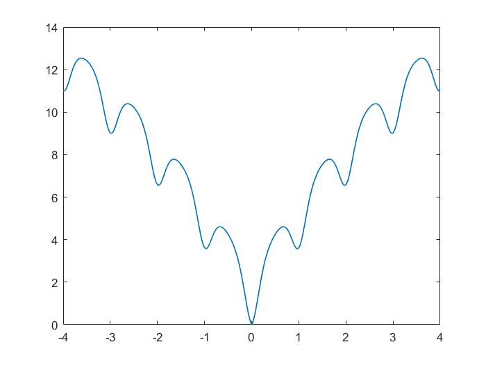
(a) Ackley

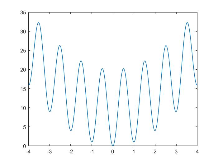
(b) Rastrigin

Figure 6.1. Benchmark functions

We implemented the ‘vanilla’ version of SBGD method $(p,q)=(1,1)$ (i.e., $\phi_{p}(\eta)=\eta$ and $\psi_{q}(\widetilde{m})=\widetilde{m}$), and with parameters $\lambda=0.2,\ \gamma=0.9,\ h_{0}=1$. Here $\lambda,\gamma$ are the descent and shrinkage parameters, and $h_{0}$ is the initial step length for backtracking line search. We record the results of $m=200$ independent simulations of Algorithm 2 with initial positions of the agents uniformly distributed in the interval $[-3,3]$.

To illustrate the behavior of the algorithm, we present the evolution of agents in one representative simulation for the Ackley function and the Rastrigin function in Figures 6.2 and 6.3, where $N=20$ agents are applied to search the domain. The blue line depicts the target function, the red circles represent the agents. It is seen that as the iterations progress, the agents flock towards different minima. The agents getting stuck at local minimizers are gradually removed due to the mass transition, while those approaching the global minimizer are eventually merged into one agent. Table 6.1 shows the results for the Ackley and the Rastrigin functions with a varying number of agents. The algorithm gives accurate solutions in all the test cases. With more agents applied the quality of the approximation is improved. However, we notice that improvement is significant as $N$ increases from 5 to 10, whereas increasing the number of agents from 10 to 20 does not result in much enhancement.

B=0		N=5	N=10	N=20
Ackley function $F_{\textnormal{Ackley}}$	success rate	$99.50\%$	$100\%$	$100\%$
	$\displaystyle{\mathbb{E}}|x_{SOL}-x^{*}|^{2}$	$4.70e^{-3}$	$8.21e^{-10}$	$6.89e^{-10}$
Rastrigin function $F_{\textnormal{Rstrgn}}$	success rate	$97.00\%$	$100\%$	$100\%$
	$\displaystyle{\mathbb{E}}|x_{SOL}-x^{*}|^{2}$	$4.45e^{-2}$	$5.18e^{-10}$	$1.89e^{-10}$

Table 6.1. Results of SBGD for 1D Ackley and Rastrigin functions, $m=200$.

The key feature of the SBGD algorithm is communication, reflected by the mass transitions between the agents. Such a mechanism dynamically adjusts the search strategies of different individuals. It is of interest to verify the benefit of communication. We compare the results by the SBGD method with those by the non-communicating multi-agents gradient descent, GD(BT), of which all the agents conduct gradient descent search independently. Tables 6.2 and 6.3 present the results by SBGD and GD(BT) methods obtained from $m=$200 experiments computed with varying shift parameter $B$ and different numbers of agents. We observe that when the initial distribution centers at $\mathbf{x}^{*}$ or is moderately shifted, both SBGD and GD(BT) methods are able to find the global minimizer. However, the advantage of SBGD is more pronounced as $\mathbf{x}^{*}$ is shifted farther away from the center of initial data, and the non-communicating GD(BT) fails to give correct solutions since its exploration is restricted to the neighborhood of its initial data. Figure 6.4 displays the scenario $B=25$, where the initial distribution is strongly shifted away from the global minimizer. The GD(BT) fails to find the global minimum. In contrast, the SBGD method employs light agents to conduct a more aggressive search in a larger area, and the algorithm ends at the correct minimizer at a surprisingly high success rate.

Remark 6.1.

Observe that when the initial data are placed far from the global minmum, the presence of a strong shift, $B=25$, requires sufficiently many swarming agents $N>20$, in order to secure a success rate $>90\%$ and drive the expected value of the error, ${\mathbb{E}}|\mathbf{x}_{SOL}-\mathbf{x}^{*}|^{2}<0.5$.

$\mathbf{x}^{*}=B$		N=10	N=20	N=30
$B=0$	success rate $\displaystyle{\mathbb{E}}|x_{SOL}-x^{*}|^{2}$	$100\%$ $8.42e^{-10}$	$100\%$ $8.37e^{-10}$	$100\%$ $3.38e^{-10}$
$B=5$	success rate $\displaystyle{\mathbb{E}}|x_{SOL}-x^{*}|^{2}$	$100\%$ $8.41e^{-10}$	$100\%$ $7.58e^{-10}$	$100\%$ $5.01e^{-10}$
$B=15$	success rate $\displaystyle{\mathbb{E}}|x_{SOL}-x^{*}|^{2}$	$98.5\%$ $1.41e^{-2}$	$100\%$ $4.69e^{-3}$	$100\%$ $8.27e^{-10}$
$B=25$	success rate $\displaystyle{\mathbb{E}}|x_{SOL}-x^{*}|^{2}$	$45.5\%$ $1.48e^{+2}$	$89.0\%$ $1.49e^{+1}$	$98.5\%$ $3.28e^{-1}$

Table 6.2. Shifted 1D Ackley, results by SBGD, $m=200$.

$\mathbf{x}^{*}=B$		N=10	N=20	N=30
$B=0$	success rate $\displaystyle{\mathbb{E}}|x_{SOL}-x^{*}|^{2}$	$100\%$ $8.60e^{-10}$	$100\%$ $1.36e^{-9}$	$100\%$ $1.29e^{-9}$
$B=5$	success rate $\displaystyle{\mathbb{E}}|x_{SOL}-x^{*}|^{2}$	$100\%$ $8.51e^{-10}$	$100\%$ $1.25e^{-9}$	$100\%$ $1.21e^{-9}$
$B=15$	success rate $\displaystyle{\mathbb{E}}|x_{SOL}-x^{*}|^{2}$	$46.5\%$ $6.44e^{+1}$	$75.0\%$ $2.26e^{+1}$	$85.5\%$ $1.14e^{+1}$
$B=25$	success rate $\displaystyle{\mathbb{E}}|x_{SOL}-x^{*}|^{2}$	$0\%$ $4.86e^{+2}$	$0\%$ $4.50e^{+2}$	$0\%$ $4.38e^{+2}$

Table 6.3. Shifted 1D Ackley, results by GD(BT) (no communication), $m=200$.

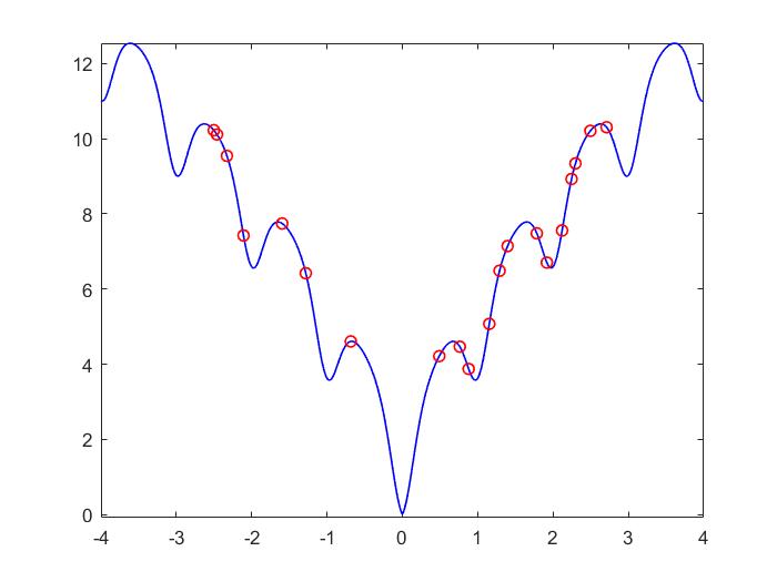
(a) Iter = 1, N = 20

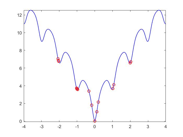
(b) Iter = 3, N = 17

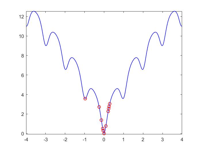
(c) Iter = 6, N = 12

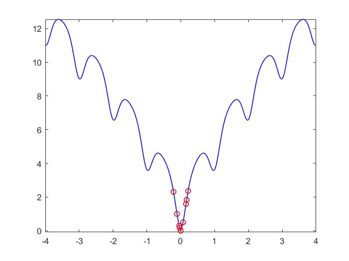
(d) Iter = 8, N = 9

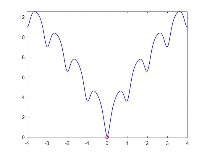
(e) Iter = 15, N = 1

Figure 6.2. 1D Ackley: evolution of agents in one simulation. $B=C=0$.

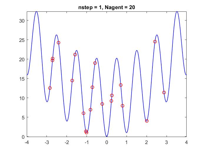
(a) Iter = 1, N = 20

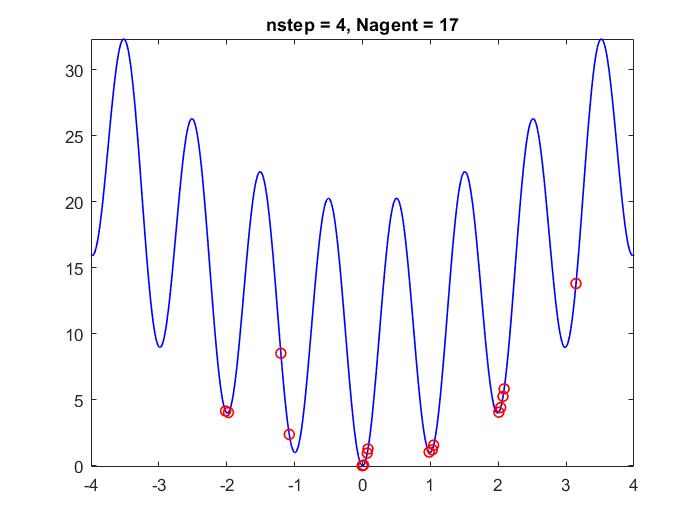
(b) Iter = 4, N = 17

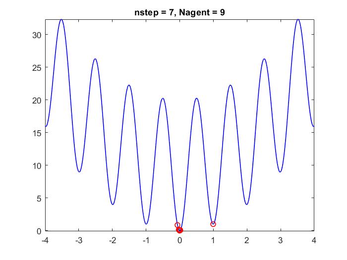
(c) Iter = 7, N = 9

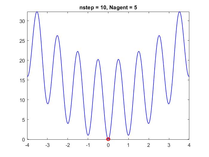
(d) Iter = 10, N = 5

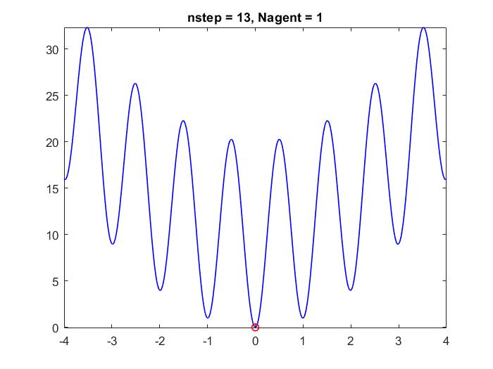
(e) Iter = 13, N = 1

Figure 6.3. 1D Rastrigin: evolution of agents in one simulation. $B=C=0$.

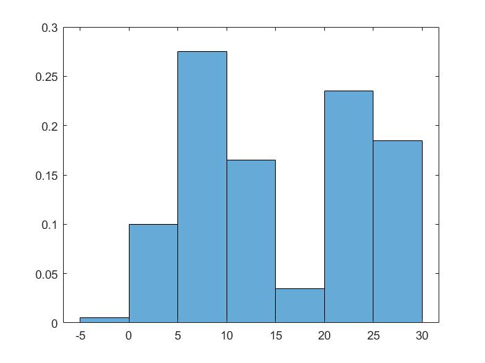
(a) SBGD, $N=10$

(b) GD(BT) , $N=10$

(c) SBGD, $N=20$

(d) GD(BT) , $N=20$

(e) SBGD, $N=20$

(f) GD(BT) , $N=20$

Figure 6.4. Histograms of the shifted 1D Ackley function by 200 experiments. $B=25$, $C=5$. Global minimum $\min F_{\textnormal{Ackley}}=5$ is attained at $\mathbf{x}_{*}=25$.

(a) Ackley

(b) Rastrigin

Figure 6.5. Histograms of 1-D optimization, $B=C=0$, 200 simulations, bin width = $10^{-4}$.

(a) Ackley: $B=2$, $C=5$, $\operatorname*{argmin}F_{A}=2$.

(b) Ackley: $B=7$, $C=5$, $\operatorname*{argmin}F_{A}=7$.

(c) Rastrigin: $B=2$, $C=5$, $\operatorname*{argmin}F_{B}=2$.

(d) Rastrigin: $B=5$, $C=5$, $\operatorname*{argmin}F_{B}=7$.

Figure 6.6. Histograms of 1D optimization with shifting, 200 simulations, bin width = $10^{-4}$.

7. Numerical results — two-dimensional problems

7.1. Optimization of parameters

Let us first comment on the general issue of optimization of parameter space. As noted in [28], once the parameterization of an adaptive GD method is fixed, it may not yield as good as or better results as simpler GD methods, yet adaptivity should be ‘judged’ after being optimized in space parameter, [6]. In this context, one can argue that optimizing a single agent method in parameter space is equivalent to a selective choice among many simulations of non-communicating multi-agent dynamics, whereas the swarm-based approach provides a dynamic, ‘on the fly’ selection of optimized parameters, which is precisely the type of comparisons we make below.

On the other hand, our SBGD method depends on several parameters: the initial step $h_{0}$, the descent parameter $\lambda$ and shrinkage parameter $\gamma$ tied to the backtracking, the tolerance parameters (3.5) and the $(p,q)$ parameters. In the multi-dimensional computations reported below, we do not optimize these SBGD parameters. Thus, unless otherwise stated, we examine the performance of the SBGD method in Algorithm 2 with initial step size $h_{0}=1$, a descent parameter $\lambda=0.2$, a shrinkage parameter $\gamma=0.9$ and the threshold parameters (3.5). We begin here with the ‘vanilla’ version of SBGD, $(p,q)=(1,1)$, although later we shall find out that the choice $(p,q)=(2,1)$ seems universally better. We run $m$ number of independent simulations, initiated with uniformly distributed positions, $\{\mathbf{x}^{0}_{i}\}$ and measure the success of the SBGD according to the proportion of its successful end results.

We illustrate the performance of the SBGD algorithm in multiple dimensions on three benchmark test cases, [11]. First, the Ackley function

(7.1) $$F_{\textnormal{Ackley}}(\mathbf{x})=-20\exp\Big{\{}-\frac{0.2}{\sqrt{d}}\Big{\{}\sum^{d}_{i=1}(\mathbf{x}_{B})_{i}^{2}\Big{\}}^{\nicefrac{{1}}{{2}}}\Big{\}}-\exp\Big{\{}\frac{1}{d}\sum^{d}_{i=1}\cos(2\pi(\mathbf{x}_{B})_{i})\Big{\}}+20+e+C.$$

Second, the Rastrigin function

(7.2) $$F_{\textnormal{Rstgin}}(\mathbf{x})=\frac{1}{d}\sum^{d}_{i=1}\Big{\{}(\mathbf{x}_{B})_{i}^{2}-10\cos(2\pi(\mathbf{x}_{B})_{i})+10\Big{\}}+C.$$

Here $d$ is the dimension of the ambient space, $\mathbf{x}_{B}:=(x_{1}-B,\ldots,x_{d}-B)$ is the shifted variable in ${\mathbb{R}}^{d}$ and $B,C\in\mathbb{R}$ are the shift parameters. Both functions attain the global minimum $C$ at the unique global minimizer $\mathbf{x}^{*}=B$.

Third, we consider the drop-wave function

(7.3) $$F_{\textnormal{Drop}}(\mathbf{x})=-\frac{1+\cos(12|\mathbf{x}|)}{0.5|\mathbf{x}|^{2}+2},$$

with SBGD parameters $\lambda=0.3,\ \gamma=0.9,\ h_{0}=1$. The agents are initialized with uniform distribution of positions in the hypercube $[-3,3]^{d}$.

To evaluate the quality of the solution, we make use of the success rate among $m$ independent simulations. We consider a simulation to be successful if $\mathbf{x}_{SOL}$ is within the $d$-dimensional cube $[\mathbf{x}^{*}-0.25,\mathbf{x}^{*}+0.25]^{d}$, e.g., [4, §4.2]. This condition ensures that the approximate solution lies in the basin of attraction of the global minimizer. In fact, in a successful experiment the solution will lie in a much smaller neighborhood of $\mathbf{x}^{*}$.

7.2. SBGD compared with non-communicating GD(BT)

We verify the advantage of the SBGD method in comparison to the non-communicating GD(BT) algorithm. We consider the three benchmarks of Ackley, Rastrigin and drop-wave functions in two dimensions. The landscapes are as shown in Figure 7.1. All functions have multiple local minimums. While the global minimum of the Ackley function is obviously lower than the other local minimums, the global minimum of the Rastrigin function is much less distinguishable. The drop-wave function has complex geometry with high frequency local minima and sharp basins of attractions. Its global minimum $F(\mathbf{x}^{*})=-1$ is attained at the unique global minimizer $\mathbf{x}^{*}=0$.

(a) 2-D Ackley

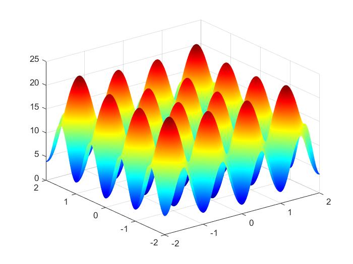
(b) 2-D Rastrigin

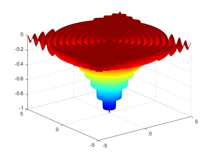
(c) 2-D drop-wave function

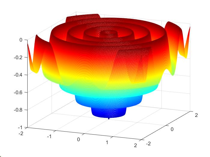
(d) zoom into 2-D drop-wave function

Figure 7.1. Landscapes of benchmark functions in two dimensions

Table 7.1 compares the success rates of SBGD and GD(BT) methods in the Ackley test cases with varying function shifts $B$ and different numbers of agents $N$. It is observed that the two methods perform comparably well when the initial distribution is centered at $\mathbf{x}^{*}$ or moderately shifted. But as the shift parameter $B$ increases, the SBGD method still achieves high success rates whereas the non-communicating GD(BT) method fails. The results for the Rastrigin function, given in Table 7.2, echo the same advantage of SBGD in shifted scenarios.

$\mathbf{x}^{*}=B$		N=25	N=50	N=100
$B=0$	SBGD GD(BT)	$98.0\%$ $100\%$	$100\%$ $100\%$	$100\%$ $100\%$
$B=5$	SBGD GD(BT)	$93.6\%$ $71.2\%$	$98.6\%$ $87.0\%$	$99.8\%$ $99.2\%$
$B=10$	SBGD GD(BT)	$66.2\%$ $0\%$	$90.8\%$ $0\%$	$98.4\%$ $0.6\%$

Table 7.1. 2D Ackley, success rates of SBGD vs. GD(BT), $m=500$.

$\mathbf{x}^{*}=B$		N=25	N=50	N=100
$B=0$	SBGD GD(BT)	$73.6\%$ $53.0\%$	$95.2\%$ $76.4\%$	$100\%$ $96.40\%$
$B=5$	SBGD GD(BT)	$44.4\%$ $15.8\%$	$80.4\%$ $28.4\%$	$99.2\%$ $56.4\%$
$B=10$	SBGD GD(BT)	$14.8\%$ $13.0\%$	$44.0\%$ $30.4\%$	$78.4\%$ $56.2\%$

Table 7.2. 2D Rastrigin, success rates of SBGD vs. GD(BT), $m=500$.

	N=10	N=20	N=30
SBGD	$90.5\%$	$99.5\%$	$100\%$
GD(BT)	$15.0\%$	$21.5\%$	$35.5\%$

Table 7.3. 2D drop-wave, success rates of SBGD vs. GD(BT), $m=500$.

${\mathbb{E}}|\mathbf{x}_{SOL}-\mathbf{x}^{*}|^{2}$	$\lambda=0.3$	$\lambda=0.5$	$\lambda=0.7$
SBGD	2.07e-1	6.18e-2	1.29e-1
GD(BT)	4.25e-2	6.08e-2	1.29e-1

Table 7.4. Average error for 2D Rosenbrock function SBGD vs. GD(BT), $m=500$ simulations equi-distributed at $[-4,-2]^{2}$.

Table 7.3 compares the success rates of SBGD and GD(BT) methods in the test case of the 2D drop-wave function, (7.3). We compare the success rates of SBGD with $\lambda=0.3$ vs. the non-communicating GD(BT) using $m=200$ simulations randomly initiated with uniform distribution at $[-3,3]^{2}$. The SBGD results reported in Table 7.3 show a remarkable improvement over the performance of GD(BT); communication helps.

The SBGD does not always offer such a decisive lead over GD(BT). In table 7.4 we compare the error of SBGD vs. GD(BT) for the 2D Rosenbrock function

(7.4) $$F_{\textnormal{Rsnbrk}}(\mathbf{x})=(1-x_{1})^{2}+100(x_{2}-x_{1}^{2})^{2}.$$

The stiffness of $F_{\textnormal{Rsnbrk}}$ near its global minimum at $\mathbf{x}^{*}=(1,1)$ produces comparable results of the swarm dynamics and non-communicating GD(BT).

7.3. SBGD_pq method — dependence of $(p,q)$ parameters

We now turn to discuss the effect of adjusting the mass transition with $\phi_{p}(\eta^{n}_{i})$ and backtracking with $\psi_{q}(\widetilde{m}^{n+1}_{i})$.
We implemented the SBGD_pq for shifted 2D Rastrigin function (7.2) with shift $B=5$, and drop-wave function (7.3) using SBGD_pq with descent parameter $\lambda=0.3$, using $N$ agents uniformly initialized at $[-3,3]^{2}$. The success rate $m=500$ simulations with different $(p,q)$ are recorded in Table 7.5.
In both cases, the results for the ‘vanilla’ SBGD, $(p,q)=(1,1)$, with a success rate of 80% and respectively 90%, are substantially improved to 97%, once we use SBGD_pq with $(p,q)=(2,\nicefrac{{1}}{{2}})$. In this case, the use of $p=2$ enforces more moderate mass transitions which seems to play a key role whenever $F$ has steep basins of attractions, while $q=\nicefrac{{1}}{{2}}$ enforces a slower marching protocol for intermediate agents.

	$\sqrt{\widetilde{m}}$	$\widetilde{m}$	$\widetilde{m}^{2}$
$\sqrt{\eta}$	77.2%	43.0%	40.0%
$\eta$	94.8%	80.4%	73.4%
$\eta^{2}$	97.8%	94.0%	88.4%
$\eta^{20}$	83.4%	95.4%	98.2%

(a) 2D Rastrigin function; $N=50$ agents

	$\sqrt{\widetilde{m}}$	$\widetilde{m}$	$\widetilde{m}^{2}$
$\sqrt{\eta}$	93.6%	83.0%	79.8%
$\eta$	97.2%	90.4%	85.2%
$\eta^{2}$	97.6%	96.0%	90.2%
$\eta^{20}$	80.8%	98.8%	97.4%

(b) 2D Drop-wave function; $N=10$ agents

Table 7.5. SBGD_pq for shifted 2D Rastrigin and drop-wave with different $(p,q)$

	$\sqrt{\widetilde{m}}$	$\widetilde{m}$	$\widetilde{m}^{2}$
$\eta$	2.53e-1	2.07e-1	1.78e-1
$\eta^{2}$	8.51e-2	3.07e-1	1.70e-1
$\eta^{20}$	6.39e-2	2.01e-1	2.74e-1
$\eta^{50}$	5.75e-2	1.88e-1	2.61e-1

(a) SBGD_pq with $\lambda=0.3$.

	$\sqrt{\widetilde{m}}$	$\widetilde{m}$	$\widetilde{m}^{2}$
$\eta$	6.79e-2	6.18e-2	6.05e-2
$\eta^{2}$	4.97e-2	7.10e-2	6.08e-2
$\eta^{20}$	4.65e-2	5.95e-2	6.74e-2
$\eta^{50}$	4.98e-2	6.02e-2	6.87e-2

(b) SBGD_pq with $\lambda=0.5$.

	$\sqrt{\widetilde{m}}$	$\widetilde{m}$	$\widetilde{m}^{2}$
$\eta$	7.11e-2	1.51e-1	1.29e-1
$\eta^{2}$	6.83e-2	1.22e-1	1.29e-1
$\eta^{20}$	1.21e-1	6.45e-2	1.48e-1
$\eta^{50}$	1.26e-1	6.76e-2	1.37e-1

(c) SBGD_pq with $\lambda=0.7$.

Table 7.6. SBGD_pq simulation of 2D Rosenbrock $F_{\textnormal{Rsnbrk}}$ with different $(p,q)$. A larger $\lambda$ enforces a stronger descent property. The parameter $p=2$ is a most effective parameterization of SBGD_pq.

As a further example we consider the 2D Rosenbrock function $F_{\textnormal{Rsnbrk}}$ in (7.4). The difficulty arises when the iterations approach the neighborhood of a global minimum $F(\mathbf{x}^{*})=0$ attained at $\mathbf{x}^{*}=(1,1)$. This is due to the severe “skew-ness” of $F$ which is sensitive to the descent parameter $\lambda$. We employ $N=30$ agents initialized with randomly distributed positions at $[-4,-2]^{2}$. Success rates are computed among $m=500$ experiments. Table 7.6 records the GD(BT) and SBGD_pq errors, measured by ${\mathbb{E}}|\mathbf{x}_{SOL}-\mathbf{x}^{*}|^{2}$, for different values of descent parameter, $\lambda$, and for different protocols of $(p,q)$. The sensitive dependence on $\lambda$ is observed with both the non-communicating GD(BT) and the SBGD_pq. Once again, the parameters $(p,q)=(2,\nicefrac{{1}}{{2}})$ yield the most stable performance of SBGD_pq, whereas other scaling of GD(BT) and SBGD are more sensitive to the choice of $\lambda$.

In summary, Tables 7.5 and 7.6 indicate that while the results of SBGD_pq are mostly comparable, SBGD${}_{(2,\nicefrac{{1}}{{2}})}$ seems to provide optimal results, with main emphasize on $p=2$. At the same time, we conclude that the tuning parameters, $(pq)$, have a limited effect on the overall performance of SBGD_pq method. Accordingly, we did not optimize these parameters.
Motivated by these findings, we focus below on two versions of SBGD (see also Tables 2.1 and 2.2): the vanilla version, SBGD_1,1 with $\phi_{p}(\eta)=\eta$ and $\phi_{q}(\widetilde{m})=\widetilde{m}$, and SBGD_2,1 with $\phi_{p}(\eta)=\eta^{2}$ which seems to be a universally better.

7.4. 2D comparison with the Adam method

We report on the results of SBGD_pq, compared with the Adam method for the 2D Rastrigin function 7.2. We also include results for the GD($h$) and GD(BT) methods. As in the case of the 1D objective function (2.3), we distinguish between two cases: initial data uniformly distributed in $[-3,3]^{2}$ enclosing the global minimum at the origin, vs. initial data uniformly distributed at $[-3,-1]^{2}$. The SBGD_pq variants with $(p,q)=(1,1)$ and $(p,q)=(2,1)$ were computed for $m=1000$ simulations with random with descent parameter $\lambda=0.8$, and using tolerance parameters, $tolmerge=0.1$, $tolm=0.01$ and $tolres=10^{-4}$.
The SBGD_pq variant with $(p,q)=(2,1)$ seems consistently better than the vanilla version $(p,q)=(1,1)$. This will be further explored in the next §7.3. When the methods are initiated at $[-3,3]^{2}$, the SBGD variants provide comparable or better results than GD($h$) , GD(BT) and Adams methods. When initiated at $[-3,-1]^{2}$ which does not enclose $\mathbf{x}^{*}$, the SBGD variants provide distinctively better results than GD($h$) , GD(BT) and Adam methods. The Adam iterations with the smaller initial step size $h_{0}=0.2$ remain trapped in local basins of attraction.

N	5	10	15	20	30
SBGD11	34.4%	52.1%	62.6%	70.0%	75.8%
SBGD21	34.5%	60.1%	75.3%	84.3%	91.0%
GD(0.004)	36.3%	50.5%	60.0%	70.0%	78.1%
GD(BT)	35.0%	51.0%	62.0%	70.8%	79.3%
Adam(0.8)	23.7%	29.6%	39.1%	46.8%	65.5%
Adam(0.2)	32.1%	40.9%	55.9%	65.3%	79.4%

Table 7.7. Success rates of SBGD compared with GD($h$) , GD(BT) and Adam methods for global optimization of (7.2)($B=0$), based on $m=1000$ runs with uniformly generated initial data in $[-3,3]^{2}$.

N	5	10	15	20	30
SBGD11	17.0%	49.2%	61.7%	67.0%	72.7%
SBGD21	14.2%	46.7%	68.4%	81.9%	89.6%
GD(0.004)	0.0%	0.0%	0.0%	0.0%	0.0%
GD(BT)	1.8%	2.4%	3.4%	4.3%	5.9%
Adam(0.8)	24.5%	31.3%	41.4%	49.2%	66.9%
Adam(0.2)	0.0%	0.0%	0.0%	0.0%	0.0%

Table 7.8. Success rates of SBGD compared with GD($h$) , GD(BT) and Adam methods for global optimization of 2D Rastrigin (7.2)($B=0$) based on $m=1000$ runs of uniformly generated initial data in $[-3,-1]^{2}$.

8. Numerical results — $20$-dimensional problems

We now turn attention to the computation of the global minimizer for the 20-dimensional Rastrigin and Ackley functions. As the dimension of the ambient space to be explored increases, so does the number of agents, $N$, necessary to explore that space in order to secure a ‘faithful’ approximate minimizer. The increase of $N$ dependence on the dimension $d$ is intimately related to the way one quantifies the quality of such an approximation .

8.1. Success rate — $N$ vs. $d$

One approach to measure success that was used in one- and two-dimensional problems, is to secure a computed solution within a pre-determined neighborhood of the global minimizer, $[\mathbf{x}^{*}-0.25,\mathbf{x}^{*}+0.25]^{d}$. This approach places severe restrictions in the case of high-dimensional data. Specifically, Table 8.1 and even more so, Table 8.1, show the rapid growth in the number of SBGD agents, $N=N(d)$, which are required to ensure $80\%$ success rate in $m=500$ tests of high-dimensional Ackley, and respectively, 70% success rate in Rastrigin benchmark functions. In both cases, one observes a rather small critical dimension, $d_{c}$, such that $N(d)\gg N(d_{c})$ for $d>d_{c}$.

d	10	11	12	13	14	15	16
N	15	18	23	42	120	540	3000

(a) 80% success rate with Ackley function

d	1	2	3	4
N	4	23	180	2900

(b) 70% success rate with Rastrigin function

Table 8.1. Success rate of $\mathbf{x}_{SOL}\in[\mathbf{x}^{*}-0.25,\mathbf{x}^{*}+0.25]^{20}$.

$\mathbf{x}_{*}=B$		N=50	N=100	N=200
$B=0$	SBGD21 GD(BT) Adam(0.5)	9.00e-07 1.18e-01 3.37e-03	2.02e-07 6.90e-02 4.03e-03	1.43e-07 1.88e-02 4.96e-03
$B=3$	SBGD21 GD(BT) Adam(0.5)	1.65e-06 7.64 2.14e-01	1.51e-06 6.72 1.22e-01	7.96e-07 5.67 1.27e-01
$B=5$	SBGD21 GD(BT) Adam(0.5)	4.15 17.99 11.01	1.07 17.59 9.27	2.36e-01 17.11 7.52

Table 8.2. ${\mathbb{E}}[\mathbf{x}_{SOL}-\mathbf{x}^{*}|$ for 20-dimensional shifted Ackley. $m=1000$.

$\mathbf{x}_{*}=B$		N=50	N=100	N=200
$B=0$	SBGD21 GD(BT) Adam(0.5)	4.03e-01 2.96e-01 3.75e-01	4.98e-01 3.25e-01 2.86e-01	3.91e-01 4.35e-01 4.14e-01
$B=3$	SBGD21 GD(BT) Adam(0.5)	5.07 9.43 9.02	3.71 9.02 8.63	2.92 8.57 8.15
$B=5$	SBGD21 GD(BT) Adam(0.5)	3.53 18.02 17.13	2.45 17.64 16.73	1.29 17.18 16.3

Table 8.3. ${\mathbb{E}}[\mathbf{x}_{SOL}-\mathbf{x}^{*}|$ for 20-dimensional shifted Rastrigin. $m=1000$.

An alternative approach to quantify the quality of computed minimizers is to measure the expected (average) error in position, ${\mathbb{E}}[\mathbf{x}_{SOL}-\mathbf{x}^{*}|$. The results recorded in Tables 8.7 and 8.8 for 20-dimensional Ackley and, respectively, Rastrigin functions, indicate the advantage of SBGD₂₁ as the shift $B$ increases. But the main point to observe is that even for relatively large $N=100,200$, the results fail to faithfully capture the global minimizer. Indeed, we claim that going beyond the two examples of Ackley and Rastrigin, measuring the (average) distance to of the computed minimizers, is not necessarily an effective quantifier for the quality of an optimizer: one might need a large $N=N(d)$ before approaching a small neighborhood of the global minimizer.

8.2. Measuring the loss

A more ‘faithful’ way to measure the quality of numerical optimizers in high-dimensional data is to measure the average loss (height), ${\mathbb{E}}[F(\mathbf{x}_{SOL}]$. After all, the underlying goal is to minimize the value of $F$. In particular, one might argue that $\mathbf{x}_{SOL}$ will provide a faithful approximation whenever $F(\mathbf{x}_{SOL})-F(\mathbf{x}^{*})$ is small, even if $\mathbf{x}_{SOL}$ remains far from $\mathbf{x}_{i}^{n}$. This approach of ‘looking from above’, masks the increasing complexity with the increasing dimension.

$\mathbf{x}^{*}=B$		N=5	N=10	N=20	N=50	N=100	N=200
$B=0$	SBGD21 GD(BT) Adam(0.5)	54.30 53.43 48.66	43.74 44.62 44.02	39.34 39.43 37.35	34.55 34.55 32.65	32.01 31.85 30.46	33.95 29.53 27.76
$B=1$	SBGD21 GD(BT) Adam(0.5)	65.75 64.86 56.02	53.24 53.98 50.35	47.14 47.1 42.56	40.90 40.77 37.69	37.20 37.06 34.58	33.95 33.57 31.79
$B=3$	SBGD21 GD(BT) Adam(0.5)	189.24 187.8 164.46	166.46 167.58 146.82	149.14 152.46 137.16	121.45 122.35 122.84	102.98 125.44 115.16	94.77 115.83 105.5
$B=5$	SBGD21 GD(BT) Adam(0.5)	463.09 465.42 411.77	387.88 434.9 381.19	254.23 409.11 364.68	200.34 381.42 339.81	160.62 362.54 325.86	142.22 345.52 309.99

Table 8.4. 20D Rastrigin. Average loss with $m=1000$ simulations.

$\mathbf{x}^{*}=B$		N=10	N=20	N=50	N=100	N=200
$B=0$	SBGD21 GD(BT) Adam(0.5)	0.89 2.76 0.37	2.62e-05 1.92 0.073	1.17e-05 0.97 0.061	9.72e-07 0.41 0.061	1.82e-07 7.73e-02 0.061
$B=1$	SBGD21 GD(BT) Adam(0.5)	2.38 3.01 0.87	0.27 2.00 0.17	3.9e-05 0.92 0.061	6e-06 0.31 0.061	1e-06 5,45e-02 0.061
$B=3$	SBGD21 GD(BT) Adam(0.5)	7.67 7.91 3.74	4.41 7.47 2.65	0.72 6.81 1.70	0.06 6.13 1.22	5.4e-05 5.37 0.79
$B=5$	SBGD21 GD(BT) Adam(0.5)	12.01 11.98 10.72	11.49 11.8 9.70	10.01 11.53 8.45	8.47 11.36 7.58	7.09 11.17 6.67

Table 8.5. 20D Ackley. Average loss with $m=1000$ simulations.

We begin, in Table 8.4, where we record the average ‘loss’ obtained by SBGD₂₁, GD(BT) and Adam(0.5) with initial data equi-distributed in $[-3,3]^{2}$ for the 20-dimensional Rastrigin function. SBGD₂₁ was used with descent parameter $\lambda=0.8$, shrinkage parameter $\gamma=0.5$ and thresholds

$$tolmerge=\textnormal{1e-1},\ \ tolm=\textnormal{1e-3},\ \ tolres=\textnormal{1e-2}.$$

The reason for the smaller shrinkage parameter $\gamma=0.5$ was efficiency: backtracking is accelerated with more rough backtracking steps, yet this does not seem to deteriorate the quality of SBGD results. As indicated before, the results for SBGD₁₁ were only slightly worse than but otherwise comparable to SBGD₂₁ and therefore are not recorded here. We make two observations.

(i) For a small number of agents, $N\leqslant 10$, the results, particularly SBGD₂₁ and GD(BT) are comparable. Indeed, we recall that SBGD eliminates the lightest agents, so that after $N-1$ iterations, it is left with a single agent which explores the large, uncharted ambient space, much like a single-agent method.
(ii) There is a clear trend that we saw before: SBGD₂₁ outperforms the non-communicating GD(BT) and Adam when the global minimum is not enclosed within the initial domain of initial data. While the results are comparable for $B=0,1$ and/or small $N$’s, there is an increasing difference for $B=3,5$ and $N>20$.

Finally, in Table 8.5 we report on the corresponding comparison of average loss for the 20-dimensional Ackley function. Here, one encounters a much more sensitive dependence on the initial step size: we had to increase $h_{0}=2$ (instead of $h_{0}=1$ used before) in order to realize the advantage of SBGD₂₁. We maintain the usual backtracking parameters $\lambda=0.2$ and $\gamma=0.9$, and threshold parameters

$$tolmerge=\textnormal{1e-3},\ \ tolm=\textnormal{1e-4},\ \ tolres=\textnormal{1e-4}.$$

8.3. SBGD as pre-conditioner

A more practical strategy is to take the expected value, ${\mathbb{E}}[\mathbf{x}_{SOL}]$, varying overall SBGD solutions resulted from $m$ randomly generated initial configurations, as a good initial guess and then iterate it with the steepest descent correction. In this way, the algorithm is expected to mimic the convergence in expectation $\displaystyle{\mathbb{E}}[\mathbf{x}_{SOL}]\stackrel{{\scriptstyle n\rightarrow\infty}}{{\longrightarrow}}\mathbf{x}^{*}$. Table 8.6 records the $L^{\infty}-$distance between the expectation ${\mathbb{E}}[\mathbf{x}_{SOL}]$ and the global minimizer $\mathbf{x}^{*}$ for the 20-dimensional Ackley and Rastrigin functions. The expectation is computed with $m=1000$ runs. We also present the error of the corrected solution $\mathbf{x}_{corr}$, which is obtained by iterating ${\mathbb{E}}[\mathbf{x}_{SOL}]$ with gradient descent until $\displaystyle|\nabla F(\mathbf{x}_{corr})|_{2}<10^{-3}$. For both benchmark functions, this strategy gives very good solutions with a reasonable amount of agents. The quality of ${\mathbb{E}}[\mathbf{x}_{SOL}]$ is improved with more agents applied.

		N=50	N=100	N=200
Ackley function	$|{\mathbb{E}}[\mathbf{x}_{SOL}]-\mathbf{x}_{*}|_{\infty}$ $|\mathbf{x}_{corr}-\mathbf{x}_{*}|_{\infty}$	$8.29e^{-2}$ $2.07e^{-13}$	$7.28e^{-2}$ $1.96e^{-13}$	$6.79e^{-2}$ $2.18e^{-13}$
Rastrigin function	$|{\mathbb{E}}[\mathbf{x}_{SOL}]-\mathbf{x}_{*}|_{\infty}$ $|\mathbf{x}_{corr}-\mathbf{x}_{*}|_{\infty}$	$2.07e^{-1}$ $9.06e^{-6}$	$7.86e^{-2}$ $2.29e^{-6}$	$7.36e^{-2}$ $2.05e^{-6}$

Table 8.6. Errors of the expectation and the corrected solution in $d=20$, $B=C=0$.

We also investigate the effect of shifting in the initial distribution. The solution $\mathbf{x}_{corr}$ is considered to be a correct approximation of global minimizer if it lies in the region $Q_{0.5}(\mathbf{x}_{*})$. Table 8.7 and 8.8 show the results for the Ackley and the Rastrigin function under varying shift parameters and different agent numbers. It turns out that the quality of the solution is very sensitive to the initial data in high dimension. The algorithm fails to work correctly in the Ackley test cases when $B=2$. The situation is even worse for the Rastrigin test cases due to the unclear difference between different minimums. The method gives wrong solutions in all the test cases when $B$ is 1.5.

$\mathbf{x}_{*}=B$		N=50	N=100	N=200
$B=1$	$|{\mathbb{E}}[\mathbf{x}_{SOL}]-\mathbf{x}_{*}|_{\infty}$ $|\mathbf{x}_{corr}-\mathbf{x}_{*}|_{\infty}$	$3.97e^{-1}$ $2.10e^{-13}$	$3.53e^{-1}$ $1.29e^{-13}$	$3.36e^{-2}$ $1.15e^{-13}$
$B=1.5$	$|{\mathbb{E}}[\mathbf{x}_{SOL}]-\mathbf{x}_{*}|_{\infty}$ $|\mathbf{x}_{corr}-\mathbf{x}_{*}|_{\infty}$	$7.45e^{-1}$ $9.69e^{-1}$	$6.78e^{-1}$ $1.27e^{-13}$	$5.43e^{-1}$ $1.60e^{-13}$
$B=2$	$|{\mathbb{E}}[\mathbf{x}_{SOL}]-\mathbf{x}_{*}|_{\infty}$ $|\mathbf{x}_{corr}-\mathbf{x}_{*}|_{\infty}$	$1.20$ $9.69e^{-1}$	$1.09$ $9.69e^{-1}$	$1.01$ $9.68e^{-1}$

Table 8.7. Solutions for the shifted Ackley function by SBGD, $d=20$, $m=1000$.

$\mathbf{x}_{*}=B$		N=50	N=100	N=200
$B=0.5$	$|{\mathbb{E}}[\mathbf{x}_{SOL}]-\mathbf{x}_{*}|_{\infty}$ $|\mathbf{x}_{corr}-\mathbf{x}_{*}|_{\infty}$	$2.21e^{-1}$ $5.86e^{-6}$	$2.38e^{-1}$ $1.06e^{-5}$	$2.24e^{-1}$ $6.53e^{-6}$
$B=1$	$|{\mathbb{E}}[\mathbf{x}_{SOL}]-\mathbf{x}_{*}|_{\infty}$ $|\mathbf{x}_{corr}-\mathbf{x}_{*}|_{\infty}$	$5.97e^{-1}$ $1.99$	$4.80e^{-1}$ $5.89e^{-6}$	$4.19e^{-1}$ $1.11e^{-5}$
$B=1.5$	$|{\mathbb{E}}[\mathbf{x}_{SOL}]-\mathbf{x}_{*}|_{\infty}$ $|\mathbf{x}_{corr}-\mathbf{x}_{*}|_{\infty}$	$7.92e^{-1}$ $9.95e^{-1}$	$7.00e^{-1}$ $9.95e^{-1}$	$6.34e^{-1}$ $1.99$

Table 8.8. Solutions for the shifted Rastrigin function by SGBD, $d=20$, $m=1000$.

The results above indicate that the solutions obtained for high-dimensional problems can be significantly affected by the shifting in the target function, especially when the global minimum is not very distinguishable from the other minima.

References

- [1] Larry Armijo. Minimization of functions having lipschitz continuous first partial derivatives. Pacific Journal of mathematics, 16(1):1–3, 1966.
- [2] Karla Ballman. Large deviations, techniques, and applications. The American Mathematical Monthly, 105(9):884, 1998.
- [3] José A Carrillo, Young-Pil Choi, Claudia Totzeck, and Oliver Tse. An analytical framework for consensus-based global optimization method. Mathematical Models and Methods in Applied Sciences, 28(06):1037–1066, 2018.
- [4] José A Carrillo, Shi Jin, Lei Li, and Yuhua Zhu. A consensus-based global optimization method for high dimensional machine learning problems. ESAIM: Control, Optimisation and Calculus of Variations, 27:S5, 2021.
- [5] Jos´e Antonio Carrillo, Claudia Totzeck, and Urbain Vaes. Consensus-based optimization and ensemble kalman inversion for global optimization problems with constraints. In Benoit Perthame Weizhu Bao, Peter A. Markowich and Eitan Tadmor, editors, Modeling and Simulation for Collective Dynamics, pages 195–230. World Scientific, 2023.
- [6] Dami Choi, Christopher J Shallue, Zachary Nado, Jaehoon Lee, Chris J Maddison, and George E Dahl. On empirical comparisons of optimizers for deep learning. arXiv preprint arXiv:1910.05446, 2019.
- [7] Sara Grassi, Hui Huang, Lorenzo Pareschi, and Jinniao Qiu. Mean-field particle swarm optimization. In Benoit Perthame Weizhu Bao, Peter A. Markowich and Eitan Tadmor, editors, Modeling and Simulation for Collective Dynamics, pages 127–194. World Scientific, 2023.
- [8] Seung-Yeal Ha, Shi Jin, and Doheon Kim. Convergence of a first-order consensus-based global optimization algorithm. Mathematical Models and Methods in Applied Sciences, 30(12):2417–2444, 2020.
- [9] Seung-Yeal Ha, Shi Jin, and Doheon Kim. Convergence and error estimates for time-discrete consensus-based optimization algorithms. Numerische Mathematik, 147(2):255–282, 2021.
- [10] John H Holland. Genetic algorithms. Scientific american, 267(1):66–73, 1992.
- [11] Momin Jamil and Xin-She Yang. A literature survey of benchmark functions for global optimisation problems. International Journal of Mathematical Modelling and Numerical Optimisation, 4(2):150–194, 2013.
- [12] Hamed Karimi, Julie Nutini, and Mark Schmidt. Linear convergence of gradient and proximal-gradient methods under the polyak-łojasiewicz condition. In Joint European Conference on Machine Learning and Knowledge Discovery in Databases, pages 795–811. Springer, 2016.
- [13] James Kennedy and Russell Eberhart. Particle swarm optimization. In Proceedings of ICNN’95-international conference on neural networks, volume 4, pages 1942–1948. IEEE, 1995.
- [14] Diederik P Kingma and Jimmy Ba. Adam: A method for stochastic optimization. arXiv preprint arXiv:1412.6980, 2017.
- [15] Scott Kirkpatrick, C Daniel Gelatt, and Mario P Vecchi. Optimization by simulated annealing. science, 220(4598):671–680, 1983.
- [16] Stanis law Lojasiewicz. Ensembles semi-analytiques. IHES notes, 1965.
- [17] Hailiang Liu and Xuping Tian. An adaptive gradient method with energy and momentum. arXiv preprint arXiv:2203.12191, 2022.
- [18] Stanislas Łojasiewicz. Sur la géométrie semi-et sous-analytique. In Annales de l’institut Fourier, volume 43, pages 1575–1595, 1993.
- [19] Jorge Nocedal and Stephen J Wright. Conjugate gradient methods. Springer, 2006.
- [20] René Pinnau, Claudia Totzeck, Oliver Tse, and Stephan Martin. A consensus-based model for global optimization and its mean-field limit. Mathematical Models and Methods in Applied Sciences, 27(01):183–204, 2017.
- [21] Boris T Polyak. Gradient methods for solving equations and inequalities. USSR Computational Mathematics and Mathematical Physics, 4(6):17–32, 1964.
- [22] Craig W Reynolds. Flocks, herds and schools: A distributed behavioral model. In Proceedings of the 14th annual conference on Computer graphics and interactive techniques, pages 25–34, 1987.
- [23] Michael Struwe. Variational methods, volume 991. Springer, 2000.
- [24] Eitan Tadmor. The large-time behavior of the scalar, genuinely nonlinear lax-friedrichs scheme. Mathematics of computation, 43(168):353–368, 1984.
- [25] Eitan Tadmor. On the mathematics of swarming: emergent behavior in alignment dynamics. Notices of the AMS, 68(4):493–503, 2021.
- [26] Claudia Totzeck. Trends in consensus-based optimization. In N. Bellomo J. A. Carrillo and E. Tadmor, editors, Active Particles, Volume 3, pages 201–226. Springer, 2022.
- [27] Peter JM Van Laarhoven and Emile HL Aarts. Simulated annealing. In Simulated annealing: Theory and applications, pages 7–15. Springer, 1987.
- [28] Ashia C Wilson, Rebecca Roelofs, Mitchell Stern, Nati Srebro, and Benjamin Recht. The marginal value of adaptive gradient methods in machine learning. Advances in neural information processing systems, 30, 2017.
- [29] Philip Wolfe. Convergence conditions for ascent methods. SIAM review, 11(2):226–235, 1969.
- [30] Xin-She Yang. Nature-inspired metaheuristic algorithms. Luniver press, 2010.