Diffusion Probabilistic Model Made Slim

Abstract

Despite the recent visually-pleasing results achieved, the massive computational cost has been a long-standing flaw for diffusion probabilistic models (DPMs), which, in turn, greatly limits their applications on resource-limited platforms. Prior methods towards efficient DPM, however, have largely focused on accelerating the testing yet overlooked their huge complexity and sizes. In this paper, we make a dedicated attempt to lighten DPM while striving to preserve its favourable performance. We start by training a small-sized latent diffusion model (LDM) from scratch, but observe a significant fidelity drop in the synthetic images. Through a thorough assessment, we find that DPM is intrinsically biased against high-frequency generation, and learns to recover different frequency components at different time-steps. These properties make compact networks unable to represent frequency dynamics with accurate high-frequency estimation. Towards this end, we introduce a customized design for slim DPM, which we term as Spectral Diffusion (SD), for light-weight image synthesis. SD incorporates wavelet gating in its architecture to enable frequency dynamic feature extraction at every reverse steps, and conducts spectrum-aware distillation to promote high-frequency recovery by inverse weighting the objective based on spectrum magni- tudes.Experimental results demonstrate that, SD achieves 8-18$\times$ computational complexity reduction as compared to the latent diffusion models on a series of conditional and unconditional image generation tasks while retaining competitive image fidelity.

1 Introduction

Diffusion Probabilistic Models (DPMs) [16, 55, 53] have recently emerged as a power tool for generative modeling, and have demonstrated impressive results in image synthesis [42, 8, 43], video generation [19, 15, 68] and 3D editing [39]. Nevertheless, the gratifying results come with a price: DPMs suffer from massive model sizes. In fact, state-of-the-art DPMs requires billions of parameters, with hundreds or even thousands of inference steps per image. For example, DALL$\cdot$ E 2 [42], which is composed of 4 separate diffusion models, requires 5.5B parameters and 356 sampling steps in total. Such enormous model size, in turn, makes DPMs extremely cumbersome to be employed in resource-limited platforms.

However, existing efforts towards efficient DPMs have focused on model acceleration but largely overlooked model lightening. For examples, the approaches of [36, 47, 34, 51, 1, 30, 33] strive for faster sampling, while those of [17, 13, 57, 43] rely on reducing the input size. Admittedly, all of these methods give rise to shortened training or inference time, yet still, the large sizes preclude them from many real-world application scenarios.

Figure 1: (1) Visualizing the frequency domain gap among generated images with the full DPM [43], Lite DPM and our SD on FFHQ [26] dataset. Lite-DPM is unable to recover fine-grained textures, while SD can produce sharp edges and realistic patterns. (2) Model size, Multiply-Add cumulation (MACs) and FID score on class-conditioned ImageNet [7]. Our model achieves compelling visual quality, with minimal parameters and computational cost. ^∗ indicates our re-implemented version.

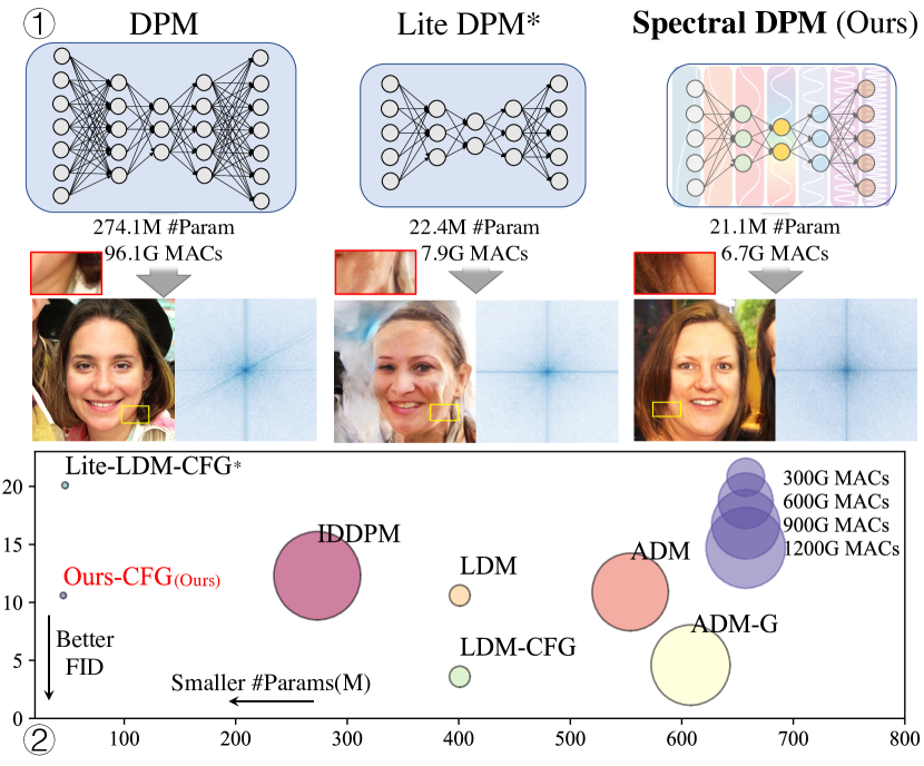
In this paper, we make a dedicated attempt towards building compact DPMs. To start with, we train a lite version of the popular latent diffusion model (LDM) [43] by reducing the channel size. We show the image generated by the original and and lite DPM in Figure 1. Although the lite LDM indeed sketches the overall structure of the faces, the high-frequency components, such as the skin and hair textures, are unfortunately poorly recovered. This phenomenon can be in fact revealed by the Discrete Fourier Transform (DFT) coefficient shown on the right column, indicating that the conventional design for DPMs leads to high-frequency deficiency when the model is made slim.

We then take an in-depth inspection on the DPMs through the lens of frequency, which results in two key observations. (1) Frequency Evolution. Under mild assumptions, we mathematically prove that DPMs learn different functionalities at different time-steps. Specifically, we show that the optimal denoiser in fact boils down to a cascade of wiener filters [61] with growing bandwidths. After recovering the low-frequency components, high-frequency features are added gradually in the later denoising stages. This evolution property, as a consequence, small DPMs fails to learn dynamic bandwidths with limited parameters. (2) Frequency Bias. DPM is biased towards dominant frequency components of the data distribution. It is most obvious when the noise amplitude is small, leading to inaccurate noise prediction at the end of the reverse process. As such, small DPMs struggle to recover the high-frequency band and image details.

Motivated by these observations, we propose a novel Spectral Diffusion (SD) model, tailored for light-weight image synthesis. Our core idea is to introduce the frequency dynamics and priors into the architecture design and training objective of the small DPM, so as to explicitly preserve the high-frequency details. The proposed solution consists of two parts, each accounting for one aforementioned observations. For the frequency evolution, we propose a wavelet gating operation, which enables the network to dynamically adapt to the spectrum response at different time-steps. In the upsample and downsample stage, the input feature is first decomposed through wavelet transforms and the coefficients are re-weighted through a learnable gating function. It significantly lowers the parameter requirements to represent the frequency evolution in the reverse process.

To compensate for the frequency bias for small DPMs, we distill the high-frequency knowledge from teacher DPM to a compact network. This is implemented by inverse weighting the distillation loss based on spectrum magnitudes. Specifically, high-frequency recovery is strengthened by over-weighting frequency bands of small magnitudes. Students thereby focus on the textual recovery for image generation. By seamlessly integrating both designs, we are able to build a slim latent diffusion model, SD, which largely preserve the performance of LDM. Notably, SD by nature inherits the merits of DPMs, including superior sample diversity, training stability and tractable parameterization. As shown in Figure 1, our model is $8\sim 18\times$ smaller and runs $2\sim 5\times$ faster than the original LDM, while achieving competitive image fidelity.

The contributions of this study are threefold:

1. This study investigates the task of diffusion model slimming, which remains largely unexplored before.

2. We identify that the key challenge lies in its unrealistic recovery for the high-frequency components. By probing DPMs from a frequency perspective, we show that there exists a spectrum evolution over different denoising steps, and the rare frequencies cannot be accurately estimated by small models.

3. We propose SD, a slim DPM that effectively restores imagery textures by enhancing high-frequency generation performance. SD achieves gratifying performance on image generation tasks at a low cost.

2 Related Work

Diffusion Probabilistic Models. DPMs [50, 16] have achieved state-of-the-art results in terms of both log-likelihood estimation [52] and sample quality [8], compared to Generative adversarial Network (GAN)-based [26, 12, 25] approaches. It has been pointed out that DPM, in its essence, is a score-based model [60, 55, 54] with annealed noise scheduling [53]. The reverse process is considered as solving reverse stochastic differential equations (SDE) [55]. Current best-performed DPMs are implemented as a time-conditioned UNet [45, 8, 55] armed with self-attention [59] and cross-attention [43, 21]. Parameter moving average [38], re-weighted objective [16] and advanced scheduling [38] significantly improves the visual quality. In this work, we focus on small diffusion designed for image generation, which has rarely been studied before.

Efficient Diffusion. The efficient diffusion model for low-resource inferences has recently become a popular research topic. One approach is through reducing the sampling steps, which is either done by distilling multiple steps into a single step [36, 47, 34], or shortening the reverse steps while maintaining the image fidelity [51, 1, 30, 33]. Another possible solution explores the idea of diffusing in a lower dimensional space , and then scaling it up, with a cascade structure [17] or in the latent space [57, 43]. In distinction from them, we build an efficient diffusion model using light-weight architecture and knowledge distillation.

Frequency Analysis for Generative Model. Neural networks tend to fit low-frequency signals first and shift to the high-frequency components, which is referred to as frequency principle of deep neural network [63, 64, 2]. The frequency bias is also observed when training deep generative models like GANs [10, 5, 27, 49], where the generator struggles to build up natural high-frequency details.

In this paper, we examine the frequency behavior of DPMs. Taking advantage of its frequency properties, our SD achieves realistic image generation at a low cost.

3 Background

3.1 Denoising Diffusion Probabilistic Models

Diffusion model reverses a progressive noise process based on latent variables. Given data $\mathbf{x}_{0}\sim q(\mathbf{x}_{0})$ sampled from the real distribution, we consider perturbing data with Gaussian noise with zero mean and $\beta_{t}$ variance for $T$ steps

$$q(\mathbf{x}_{t}|\mathbf{x}_{t-1})=\mathcal{N}(\mathbf{x}_{t};\sqrt{1-\beta_{t}}\mathbf{x}_{t-1},\beta_{t}\mathbf{I})$$ (1)

where $t\in[1,T]$ and $0<\beta_{1:T}<1$ denote the noise scale scheduling. At the end of day, $\mathbf{x}_{T}\to\mathcal{N}(0,\mathbf{I})$ converge to a Gaussian white noise. Although sampling from noise-perturbed distribution $q(\mathbf{x}_{t})=\int q(\mathbf{x}_{1:t}|\mathbf{x}_{0})d\mathbf{x}_{1:t-1}$ requires a tedious numerical integration over steps, the choice of Gaussian noise provides a close-form solution to generate arbitrary time-step $\mathbf{x}_{t}$ through

$$\mathbf{x}_{t}=\sqrt{\bar{\alpha}}\mathbf{x}_{0}+\sqrt{1-\bar{\alpha}}\bm{\epsilon},\quad\text{where}\quad\epsilon\sim\mathcal{N}(0,\mathbf{I})$$ (2)

where $\alpha_{t}=1-\beta_{t}$ and $\bar{\alpha}_{t}=\prod_{s=1}^{t}\alpha_{s}$. A variational Markov chain in the reverse process is parameterized as a time-conditioned denoising neural network $\mathbf{s}(\mathbf{x},t;\bm{\theta})$ with $p_{\bm{\theta}}(\mathbf{x}_{t-1}|\mathbf{x}_{t})=\mathcal{N}(\mathbf{x}_{t-1};\frac{1}{\sqrt{1-\beta_{t}}}(\mathbf{x}_{t}+\beta_{t}\mathbf{s}(\mathbf{x}_{t},t;\bm{\theta})),\beta_{t}\mathbf{I})$. The denoiser is trained to minimize a re-weighted evidence lower bound (ELBO) that fits the noise

$$\mathcal{L}_{\text{DDPM}} =\mathbb{E}_{t,\mathbf{x}_{0},\bm{\epsilon}}\Big{[}||\bm{\epsilon}-\mathbf{s}(\mathbf{x}_{t},t;\bm{\theta})||_{2}^{2}\Big{]}$$ (3)

$$=\mathbb{E}_{t,\mathbf{x}_{0},\bm{\epsilon}}\Big{[}||\nabla_{\mathbf{x}_{t}}\log p(\mathbf{x}_{t}|\mathbf{x}_{0})-\mathbf{s}(\mathbf{x}_{t},t;\bm{\theta})||_{2}^{2}\Big{]}$$ (4)

where the $\nabla_{\mathbf{x}_{t}}\log p(\mathbf{x}_{t}|\mathbf{x}_{0})$ are also called the score function [53]. Thus, the denoiser equivalently learns to recover the derivative that maximize the data log-likelihood [22, 60]. With a trained $\mathbf{s}(\mathbf{x},t;\bm{\theta}^{*})\approx\nabla_{\mathbf{x}_{t}}\log p(\mathbf{x}_{t}|\mathbf{x}_{0})$, we generate the data by reversing the Markov chain

$$\mathbf{x}_{t-1}\leftarrow\frac{1}{\sqrt{1-\beta_{t}}}(\mathbf{x}_{t}+\beta_{t}\mathbf{s}(\mathbf{x}_{t},t;\bm{\theta}))+\sqrt{\beta_{t}}\bm{\epsilon}_{t}$$ (5)

The reverse process could be understood as going along $\nabla_{\mathbf{x}_{t}}\log p(\mathbf{x}_{t}|\mathbf{x}_{0})$ from $\mathbf{x}_{T}$ to maximize the data likelihood.

3.2 Frequency Domain Representation of Images

Frequency domain analysis decomposes a image according to a sets of basis functions. We focus on two discrete transformations: Fourier and Wavelet Transform.

Given a $H\times W$ input signal $\mathbf{x}\in\mathbb{R}^{H\times W}$, Discrete Fourier Transform (DFT) $\mathcal{F}$ projects it onto a collections of sine and cosine waves of different frequencies and phases

$$\mathcal{X}(u,v)=\mathcal{F}[\mathbf{x}]=\sum_{x=1}^{H}\sum_{y=1}^{W}\mathbf{x}(x,y)e^{-j2\pi(\frac{u}{H}x+\frac{v}{W}y)}$$

$\mathbf{x}(x,y)$ is the pixel value at $(x,y)$; $\mathcal{X}(u,v)$ represents complex value at frequency $(u,v)$; $e$ and $j$ are Euler’s number and the imaginary unit.

On the other hand, Discrete Wavelet Transform (DWT) projects it onto multi-resolution wavelets functions. In a singlescale case, $\mathbf{x}$ is decomposed into 4 wavelet coefficients $\mathbf{x}_{\textsf{LL}},\mathbf{x}_{\textsf{LH}},\mathbf{x}_{\textsf{HL}},\mathbf{x}_{\textsf{HH}}=\textsf{DWT}(\mathbf{X})$ with halving the scale, where $\mathbf{x}_{\{\textsf{LL},\textsf{LH},\textsf{HL},\textsf{HH}\}}\in\mathbb{R}^{\frac{H}{2}\times\frac{W}{2}}$. $\mathbf{x}_{\textsf{LL}}$ stands for low-frequency component and $\mathbf{x}_{\{\textsf{LH},\textsf{HL},\textsf{HH}\}}$ are high-frequency components that contains the textural details. The coefficients could then be inverted and up-sampled back to the original input $\mathbf{x}=\textsf{IDWT}(\mathbf{x}_{\textsf{LL}},\mathbf{x}_{\textsf{LH}},\mathbf{x}_{\textsf{HL}},\mathbf{x}_{\textsf{HH}})$.

4 Frequency Perspective for Diffusion

In general signal processing, denoising is often performed in frequency space. Similar to Figure 1, Table 1 compares Low-freq and High-freq error for different DPMs on FFHQ dataset. Lite-LDM performs poorly due to its lack of high-frequency generation.

Method	#Param	FID$\downarrow$	Low-freq Error$\downarrow$	High-freq Error$\downarrow$
LDM	274.1M	5.0	0.11	0.75
Lite-LDM	22.4M	17.3	0.28(+0.17)	3.35(+2.17)

Table 1: Low-freq and High-freq error for different model size.

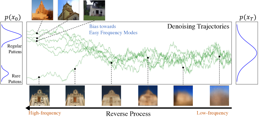
Thus, we examine DPM’s behavior in the frequency domain. As illustrated in Figure 2, we make two findings: (1) Frequency Evolution. Diffusion model learns to recover the low-frequency components at first, and gradually adds in photo-realistic and high-frequency details. (2) Frequency Bias. Diffusion model makes biased recovery for the minority frequency band.

Figure 2: Illustration of the Frequency Evolution and Bias for Diffusion Models. In the reverse process, the optimal filters recover low-frequency components first and add on the details at the end. The predicted score functions may be incorrect for rare patterns, thus failing to recover complex and fine-grained textures.

4.1 Spectrum Evolution over Time

DPM optimizes a time-conditioned network to fit noise at multiple scales, which gives rise to a denoising trajectory over time-steps. We take a close look at this trajectory through the lens of frequency. When assuming the network is a linear filter, we give the optimal filter in terms of its spectrum response at every timestep. This filter is commonly known as Wiener filter [61].

Proposition 1. Assume $\mathbf{x}_{0}$ is a wide-sense stationary signal and $\bm{\epsilon}$ is white noise of variance $\sigma^{2}=1$. For $\mathbf{x}_{t}=\sqrt{\bar{\alpha}}\mathbf{x}_{0}+\sqrt{1-\bar{\alpha}}\bm{\epsilon}$, the optimal linear denoising filter $h_{t}$ at time $t$ that minimize $J_{t}=\|h_{t}\ast\mathbf{x}_{t}-\bm{\epsilon}\|^{2}$ has a closed-form solution

$$\mathcal{H}_{t}^{*}(f)=\frac{1}{\bar{\alpha}|\mathcal{X}_{0}(f)|^{2}+1-\bar{\alpha}}$$ (6)

where $|\mathcal{X}_{0}(f)|^{2}$ is the power spectrum of $\mathbf{x}_{0}$ and $\mathcal{H}^{*}_{t}(f)$ is the frequency response of $h_{t}^{*}$.

Although the linear assumption poses a strong restriction on the model architecture, we believe it provides valuable insights into what has been done in the reverse process.

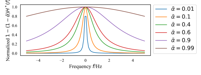
DPM goes from structure to details. In this study, we make a widely accepted assumption about the power spectra of natural images $\mathbb{E}[|X_{0}(f)|^{2}]=A_{s}(\theta)/f^{\alpha_{S}(\theta)}$that follows a power law [58, 3, 9, 56]. $A_{s}(\theta)$ is called an amplitude scaling factor and $\alpha_{S}(\theta)$ is the frequency exponent. If we set $A_{s}(\theta)=1$ and $\alpha_{S}(\theta)=2$, the frequency response of the signal reconstruction filter $1-\sqrt{1-\bar{\alpha}}h$ is in Figure 3.

In the reverse process, $t$ goes from $T\to 0$, and $\bar{\alpha}$ increases from $0\to 1$. Therefore, DPM displays a spectrum-varying behavior over time. In the beginning, we have a narrow-banded filter ($\bar{\alpha}=0.1$ and $\bar{\alpha}=0.01$) that only restores the low-frequency components that control the rough structures. $t$ goes down and $\bar{\alpha}$ gradually increases, with more details and high-frequency components restored in the images, like the human hairs, wrinkles, and pores.

We plot the denoised predictions $\hat{\mathbf{x}}_{0}$ at different steps using pre-trained LDM [43] in Figure 2, which shows that DPM generates low-frequency first and transits into high-frequency. The same empirical observation that DPM goes from rough to details has been shown in [16, 35, 6, 43], while we are the first to give its numerical solutions.

Figure 3: $1-(1-\bar{\alpha})|H^{*}(f)|^{2}$ of the optimal linear denoising filter with different $\bar{\alpha}$.

Figure 4: Toy example for 1D signal fitting. Small DPM is unable to recover minority frequency components.

4.2 Frequency Bias in Diffusion Model

Another challenge in diffusion-based model is the inaccurate denoising estimation in low-density regions [53]. It results from the expectation over $p(\mathbf{x}_{0})$ in the loss function

$$\mathcal{L}_{\text{DDPM}}=\int p(\mathbf{x}_{0})\mathbb{E}_{t,\bm{\epsilon}}\Big{[}||\bm{\epsilon}-\mathbf{s}(\mathbf{x}_{t},t;\bm{\theta})||_{2}^{2}\Big{]}\text{d}\mathbf{x}_{0}$$ (7)

Since the denoising objective is weighted by $p(\mathbf{x}_{0})$, the trained diffusion will be biased towards the high-density region, while ignoring the long-tail patterns.

For image generation tasks, one long-tail pattern is the frequency bias. While the low-frequency images are dominant with large $p(\mathbf{x}_{0})$, very few samples contain high-frequency components. Training small DPMs on the biased data distribution makes it difficult to generate samples with complex textures and realistic high-frequency patterns.

Example 1. We fit a toy diffusion model to 1D functions $f(x)=cos(\alpha 2\pi x)$, where $P(\alpha=3)=0.2$ and $P(\alpha=5)=0.8$. We adopt a two-layer feed-forward neural network, with 1000 denoising steps and hidden units $M=\{64,1024\}$. More details in in Supplementary.

We plot the 300 generated signals in Figure 4 (Top), their DFT magnitudes in (Button Right), and the mean frequency histogram in (Button Left). Small model ($M=64$) faces difficulty recovering the minority frequencies other than $\alpha=3$, while large model ($M=1024$) achieves smooth denoised results over all freq bands, especially when $\alpha=5$.

It provides concrete evidence that small DPMs have intrinsic defects in recovering the high frequencies.

5 Spectral Diffusion Model

As explained above, our goal is to slim down the DPMs by introducing the frequency dynamics and priors into the architecture design and training objectives. Taking the LDM [43] as our baseline, we design a wavelet-gating module to enable time-dynamic inference for the network with a limited model size. A spectrum-aware distillation is applied to enhance the high-frequency generation performance. Both modifications allow us to achieve photo-realistic image generation with minimal model size and computational effort.

5.1 Dynamic Wavelet Gating

As depicted in Section 4.1, the reverse process requires a cascade of filters with dynamic frequency response. Vanilla UNet [45], while being effective in reconstructing image details, is incapable to incorporate dynamic spectrum into a single set of parameters. As a result, the small-size DPM is incapable to compensate for the changing bandwidth.

In response to such frequency evolution, we propose to insert the Wavelet Gating (WG) module into the network to automatically adapt it to varing frequency response. WG decomposes the feature map into wavelet bands and selectively attends to the proper frequency at different reverse steps, which is uniquely tailored for the diffusion model.

Gating over the Wavelet Coefficients. We replace all down-sample and up-sample in UNet with DWT and IDWT [11, 65], and pose a soft gating operation on wavelet coefficients to facilitate step-adaptive image denoising. We call them WG-Down and WG-Up, as shown in Figure 5.

Following the channel attention operation [62, 20, 40], information from input feature $\mathbf{X}$ is aggregated to produce a soft gating mask

$$g_{\{\textsf{LL},\textsf{LH},\textsf{HL},\textsf{HH}\}} =\text{Sigmoid}(\text{FFN}(\text{Avgpool}(\mathbf{X})))$$ (8)

where $g_{i}$ is the gating score of each wavelet band; FFN is a 2 layer where feed-forward network and Avgpool stands for the average pooling. The coefficients are then gated with $g_{i}$ to produce the output $\mathbf{X}^{\prime}$.

Figure 5: WG-Down and WG-Up with wavelet gating.

In the WG-Down, we apply WG after the DWT operation to fuse the sub-band coefficients with weighted summation $\mathbf{X}^{\prime}=\sum_{i\in\{\textsf{LL},\textsf{LH},\textsf{HL},\textsf{HH}\}}g_{i}\odot\mathbf{X}_{i}$, where $\odot$ is the element-wise multiplication. In the WG-Up, the input feature is splitted into 4 chunks as the wavelet coefficients. Then, WG is carried out to re-weight each sub-band before $\mathbf{X}^{\prime}=\textsf{IDWT}(g_{\textsf{LL}}\odot\mathbf{X}_{\textsf{LL}},g_{\textsf{LH}}\odot\mathbf{X}_{\textsf{LH}},g_{\textsf{HL}}\odot\mathbf{X}_{\textsf{HL}},g_{\textsf{HH}}\odot\mathbf{X}_{\textsf{HH}})$. In this paper, we apply Haar wavelet by default.

5.2 Spectrum-Aware Knowledge Distillation

Diffusion model has difficulty in modelling the high-frequency components (in Section 4.2), especially for efficient requirements. In combat with spectrum deficiency in image generation, we distill the prediction of a large pre-trained teacher model to a compact WG-Unet student. Beyond output matching with a L2 loss, a Spectrum-Aware Distillation is applied to guide the student to synthesize naturalistic image details. Our intuition is to re-weight the distillation loss according to the spectrum magnitude. For components with low magnitudes, such as high-frequency bands, we increase the error penalty; while the weight for the low-frequency elements is reduced.

Suppose a teacher diffusion model $\bm{s}_{T}(\cdot;\bm{\theta}_{T})$, we would like to distill a student $\bm{s}_{T}(\cdot;\bm{\theta}_{T})$ by mimicking the outputs and features . At time-step $t$, the perturbed image $\textbf{x}_{t}$ is fed into both networks to produce the outputs and features. A L2 loss [44, 31] is use to quantify their spatial distance

$$\mathcal{L}_{\text{spatial}}=\sum_{i}\|\mathbf{X}^{(i)}_{T}-\mathbf{X}^{(i)}_{S}\|_{2}^{2}$$ (9)

where $\mathbf{X}^{(i)}_{T}$ and $\mathbf{X}^{(i)}_{S}$ stand for the pair of teacher/student’s output features or outputs of the same scale. A single 1$\times$1 Conv layer is used to align the dimensions between a prediction pair.

In addition to the spatial distillation, inspired by the imbalanced learning [28, 4, 23] and long-tail learning [67, 24], we design a distillation loss to encourage the model for minority frequency recovery. Given a pair of model predictions and the clean image $\mathbf{x}_{0}$, we first interpolate $\mathbf{x}_{0}$ to the same size of the feature map, then take their 2D DFT

$$\mathcal{X}^{(i)}_{T}=\mathcal{F}[\mathbf{X}^{(i)}_{T}],\mathcal{X}^{(i)}_{S}=\mathcal{F}[\mathbf{X}^{(i)}_{S}],\mathcal{X}^{(i)}=\mathcal{F}[\text{Resize}(\mathbf{x}_{0})]$$ (10)

The $\mathcal{X}_{0}$ is then applied to modulate the difference between $\mathcal{X}^{(i)}_{T}$ and $\mathcal{X}^{(j)}_{S}$

$$\mathcal{L}_{\text{freq}}=\frac{}{}\sum_{i}\omega_{i}\|\mathcal{X}^{(i)}_{T}-\mathcal{X}^{(j)}_{S}\|_{2}^{2},\text{where }\omega=|\mathcal{X}^{(i)}|^{\alpha}$$ (11)

with a scaling factor $\alpha<0$ ($\alpha=-1$ in our experiment), $\mathcal{L}_{\text{freq}}$ pushes the student towards learning the minority frequencies yet down-weights the majority components. Together with the DDPM objective in Eq. 3, our training objective becomes $\mathcal{L}=\mathcal{L}_{\text{DDPM}}+\lambda_{s}\mathcal{L}_{\text{spatial}}+\lambda_{f}\mathcal{L}_{\text{freq}}$ with weighting factors $\lambda_{s}=0.1$ and $\lambda_{f}=0.1$.

Note that our method aims to learn accurate score prediction at each denoising step, which is orthogonal to existing distillation on sampling step reduction [47, 36].

6 Experiments

This section demonstrates the ability of our approach SD on high-resolution image synthesis (Section 6.1) with limited computation, and validates the significance of each proposed module via ablation study in Section 6.2.

FFHQ $256\times 256$
Model	#Param	MACs	FID$\downarrow$
DDPM [16]	113.7M	248.7G	8.4
P2 [6]	113.7M	248.7G	7.0
LDM [43]	274.1M	96.1G	5.0
Lite-LDM	22.4M($12.2\times$)	7.9G($12.2\times$)	17.3($-12.3$)
Ours	21.1M($13.0\times$)	6.7G($14.3\times$)	10.5($-5.5$)

CelebA-HQ $256\times 256$
Model	#Param	MACs	FID$\downarrow$
Score SDE [55]	65.57M	266.4G	7.2
DDGAN [57]	39.73M	69.9G	7.6
LDM [43]	274.1M	96.1G	5.1
Lite-LDM	22.4M($12.2\times$)	7.9G($12.2\times$)	14.3($-9.2$)
Ours	21.1M($13.0\times$)	6.7G($14.3\times$)	9.3($-4.2$)

LSUN-Bedroom $256\times 256$
Model	#Param	MACs	FID$\downarrow$
DDPM [16]	113.7M	248.7G	4.9
IDDPM [38]	113.7M	248.6G	4.2
ADM [8]	552.8M	1114.2G	1.9
LDM [43]	274.1M	96.1G	3.0
Lite-LDM	22.4M($12.2\times$)	7.9G($12.2\times$)	10.9($-7.9$)
Ours	21.1M($13.0\times$)	6.7G($14.3\times$)	5.2($-2.2$)

LSUN-Church $256\times 256$
Model	#Param	MACs	FID$\downarrow$
DDPM [16]	113.7M	248.7G	4.9
IDDPM [38]	113.7M	248.6G	4.3
ADM [8]	552.8M	1114.2G	1.9
LDM [43]	295.0M	18.7G	4.0
Lite-LDM	32.8M($9.0\times$)	2.1G($8.9\times$)	13.6($-9.6$)
Ours	33.8M($8.7\times$)	2.1G($8.9\times$)	8.4($-4.4$)

Table 2: Unconditional generation results comparison to prior DPMs. The results are taken from the original paper, except that DDPM is take from the [6].

Figure 6: Throughput for unconditional image generation.

Datasets and Evaluation. We evaluate our model on 4 unconditional generation datasets and 2 conditional benckmarks. Specially, we train our unconditional SSD models on LSUN-Churches/Bedrooms [66], FFHQ [26], and CelebA-HQ [25]. We also validate the model on class-conditioned ImageNet [7] and MS-COCO [29] text-to-image generation. For the text-to-image task, we first train on LAION-400M [48] and test on MS-COCO directly.

Training and Evaluation Details. We build our model on the LDM [43] frameworks. All pre-trained teachers and auto-encoders are downloaded from the official repository. For fair comparison, we implement a lite-version of LDM, with a channel dimension of $64$ as our baseline model. We call it Lite-LDM.

On 4 unconditional benchmarks, we train our spectral diffusion for 150k iterations with a mini-batch size of $512$. We use AadmW [32] optimizer with initial learning rate $1.024\text{\times}{10}^{-3}$ and linear lr decay. For the class- and text-conditioned generation, the initial learning rate is set to $5.12\text{\times}{10}^{-4}$ instead, with other parameters unchanged. Classifier-free guidance [18] is applied. The synthesized image quality is measured by the FID score [14] with 50k generated samples at the resolution of $256$. We use a 200-step DDIM [51] sampling by default. We also compare the model size and computational cost in terms of parameter number and Multiply-Add cumulation (MACs). Throughput is reported as our measurement of running speed. All experiments are run on 8 NVIDIA Tesla V100 GPUs. More details are specified in the Supplementary Material.

Figure 7: Randomly sampled $256\times 256$ images generated by our models trained on CelebA-HQ [25], FFHQ [26], LSUN-Bedroom and LSUN-Church [66], ImageNet [7]. All images are sampled with 200 DDIM steps.

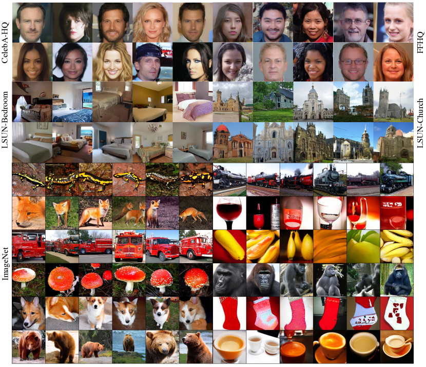
6.1 Image Generation Results

Unconditional Image Generation. We train our SD on LSUN-Churches/Bedrooms [66] FFHQ [26], and CelebA-HQ [25], and evaluate the sample quality. As shown in Table 2, directly training small-sized diffusion models largely deteriorates the model performance, such that Lite-LDM achieves an FID drop of $12.3$ on FFHQ and $13.2$ on CelebA-HQ. Our proposed SD achieves $8\sim 14$ times parameter and computation reduction compared to official LDM while being competitive in image fidelity. For example, with a 21.1M Unet model and 6.7G MACs, our SD gets an FID score of 5.2, which is very close to the 4.9 FID in DDPM, but with only $\frac{1}{37}$ of its computation cost.

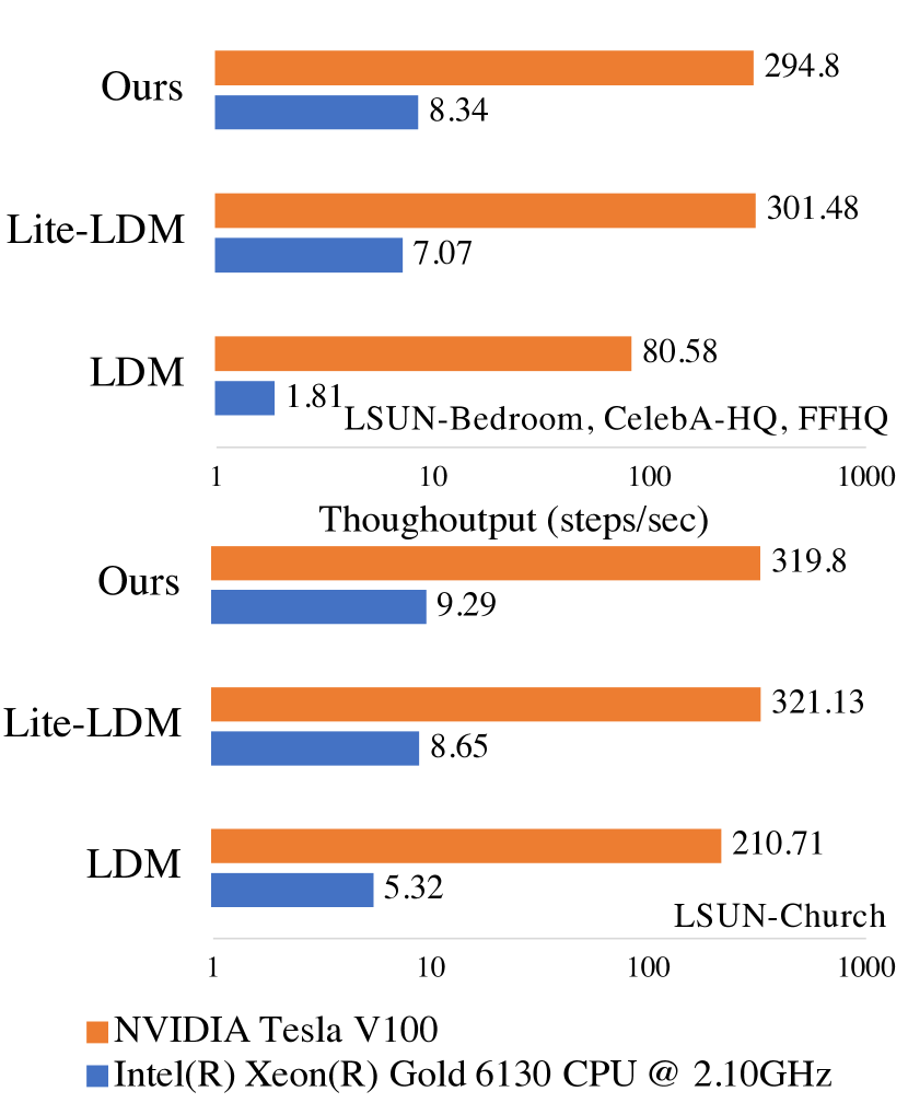
Throughput is reported in Figure 6. It refers to the number of time steps that model runs per second. We measure its value with a batch-size of 64 by averaging over 30 runs. We see that, Lite-LDM, while being fast, suffer greatly from low visual quality. In comparison, our SD is $4.6\times$ faster on CPU and $3.6\times$ on GPU compared to LDM on 3 of the 4 datasets.

We inspect the visual quality of the synthesized sample in Figure 7, row 1-4. With much less parameters and complexity, our SD still produces realistic samples with decent high-frequency details and sample diversity.

Class-conditional Image Generation. We validate our performance for class-conditioned image generation on ImageNet. The results are demonstrated in Table 3. With super-mini architecture and classifier-free guidance of $w=3.0$, our SD reaches an FID score of 10.6. As the comparison, the ADM [8] only gets FID=10.9, but with 553.8M parameters and 1114.2 MACs. Lite-LDM, though being comparably fast, suffers from its inability for high-frequency generation, gets a high FID score of 20.1.

Generated results are visualized in Figure 7 row 5-10. Our SD is able to produce diverse images of different categories, particularly good at animal generation like corgi and bear. However, we still observe failure cases with distorted faces and shapes. For example, our models suffer in crowded instance generation such as on banana.

Method	#Param	MACs	FID$\downarrow$
IDDPM [38]	273.1M	1416.3G	12.3
ADM [8]	553.8M	1114.2G	10.9
LDM [43]	400.9M	99.8G	10.6
ADM-G [8]	553.8+54.1M	1114.2+72.2G	4.6
LDM-CFG [43]	400.9M	99.8G	3.6
Lite-LDM-CFG	47.0M($8.5\times$)	11.1G ($9.0\times$)	20.1($-16.5$)
Ours-CFG	45.4M($8.8\times$)	9.9G ($10.1\times$)	10.6($-7.0$)

Table 3: Comparison of class-conditional image generation methods on ImageNet [7] with recent state-of-the-art methods. “G” stands for the classifier guidance and “CFG” refers to the classifer-free guidance for conditional image generation.

Method	#Param	FID$\downarrow$
GLIDE [37]	5.0B	12.24
DALLE2 [42]	5.5B	10.39
Imagen [46]	3.0B	7.27
LDM [43]	1.45B	12.63
Ours	77.6M($18.7\times$)	18.43

Table 4: Zero-Shot evaluation on MS-COCO text-to-image generation. We only count the model size of diffusion part but exclude language encoder.

Figure 8: Selected samples from Spectral Diffusion using classifier-free guidance $w=5.0$ for text-to-image generation.

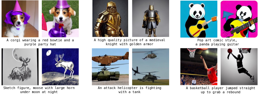
Text-to-Image Generation. Following prior work [43], we train our text-conditioned SD with a fixed CLIP encoder [41] on LAION-400M [48], and then do zero-shot inference on MS-COCO [29] with $w=2.0$. Since each MS-COCO images contains multiple captions, during evaluations, we randomly select 50k descriptions from the train set, with one caption corresponding to a unique image.

The evaluation results are provided in Table 4. Again, with a 77.6M model, we gets to a FID score of 18.43, while being $18.7\times$ smaller than LDM. We also provide qualitative analysis for text-to-image generation with new prompts, in Figure 8. Although the image quality is not as perfect as in those large-sized diffusion models, our model learns to compose vivid drawing according to the descriptions, with minimal computational cost and portable model size. Our SD is good at abstract or carton style paintings. However, it is still challenging to generate human body and faces, as in the “basketball player” example.

6.2 Ablation Study and Analysis

In this section, we validate the effectiveness of wavelet gating and spectrum-aware distillation, on whether and how they help to improve the image fidelity.

Effectiveness of Wavelet Gating. We validate the effectiveness of the Wavelet Gating by replacing our WG upsample and downsample with the nearest neighbor resizer in LDM [43] and train on the FFHQ dataset. As shown in Table 5, removing WG significantly increases the FID from $10.5\to 12.4$. Besides, WG alone improves Lite-LDM’s FID score by $2.6$. Both results indicate that WG

effectively promote the sample quality of the small DPMs.

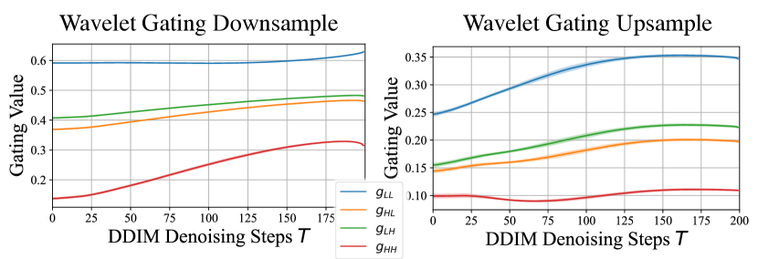
In addition, we plot the values of the gating functions at different denoising steps for a pre-trained text-to-image SD model in Figure 9. Each curve is calculated by averaging the gating coefficient for 100 generated images. The trends of the downsample and upsample operations diverge. In the end of denoising (large $t$), high-frequency details emerged in $\hat{\mathbf{x}}_{t}$. The WG-Down thus enhances the high-frequency signals with increased $g_{\{\textsf{HL},\textsf{LH},\textsf{HH}\}}$ while keeping the low-frequency part constant. In contrast, the WG-Up (Right) promotes $g_{\textsf{LL}}$ in the late stage of denoising. Predicted noises boost its low-frequency components, resulting in high-frequency element recovery in the $\hat{\mathbf{x}}_{0}=\frac{\mathbf{x}_{t}-\sqrt{1-\bar{\alpha}\bm{\epsilon}}}{\sqrt{\bar{\alpha}}}$.

Effectiveness of Spectrum-Aware Distillation. To understand the value of the proposed SA-Distillation, we sequentially remove each loss term. Figure 5 shows that, while the spatial term only accounts for 0.9 FID, the frequency term takes up 1.8 FID improvement, highlighting its importance in high-quality image generation.

We also visualize the images generated by trained models with (W) or without (W/O) the frequency term in Figure 10, with their DFT difference. The model without $\mathcal{L}_{freq}$ makes smoother predictions, while our method recovers the details like hair or architectural textures. By penalizing high-frequency distillation, our proposed SA-Distillation resulted in large differences and improvements in high-frequency components in $|\mathcal{F}_{f}-\mathcal{F}_{nof}|$.

Method	FFHQ $256\times 256$
+ Wavelet Gating		✓			✓		✓	✓
+ Spatial Distill			✓		✓	✓		✓
+ Freq Distill				✓		✓	✓	✓
FID$\downarrow$	17.3	14.7	16.6	15.3	12.3	12.4	11.4	10.5

Table 5: Ablation study on FFHQ dataset.

Figure 9: Wavelet gating function values at different $t$. We plot the mean$\pm$std for 100 generated images.

Figure 10: Generated images W or W/O the freq term, as well as their DFT difference $|\mathcal{F}_{\text{f}}-\mathcal{F}_{\text{nof}}|$.

7 Conclusion

In the study, we focus on reducing the computation cost for diffusion models. The primary obstacle to training small DPMs is their inability to provide realistic high-frequency, which results from the frequency evolution and bias of diffusion process. In order to resolve these problems, we propose Spectral Diffusion (SD) for efficient image generation. It performs spectrum dynamic denoising by using a wavelet gating operation, which automatically enhances different frequency bands at different reverse steps. A large pre-trained network helps to improve the performance of high-frequency generation by knowledge distillation. By seamlessly integrating both modifications, our model is 8-18 $\times$ slimer and runs 2-5$\times$ faster than the latent diffusion model, with negligible performance drop.

References

- [1] Fan Bao, Chongxuan Li, Jun Zhu, and Bo Zhang. Analytic-dpm: an analytic estimate of the optimal reverse variance in diffusion probabilistic models. arXiv preprint arXiv:2201.06503, 2022.
- [2] Ronen Basri, Meirav Galun, Amnon Geifman, David Jacobs, Yoni Kasten, and Shira Kritchman. Frequency bias in neural networks for input of non-uniform density. In International Conference on Machine Learning, pages 685–694. PMLR, 2020.
- [3] Geoffrey J Burton and Ian R Moorhead. Color and spatial structure in natural scenes. Applied optics, 26(1):157–170, 1987.
- [4] Kaidi Cao, Colin Wei, Adrien Gaidon, Nikos Arechiga, and Tengyu Ma. Learning imbalanced datasets with label-distribution-aware margin loss. Advances in neural information processing systems, 32, 2019.
- [5] Yuanqi Chen, Ge Li, Cece Jin, Shan Liu, and Thomas Li. Ssd-gan: Measuring the realness in the spatial and spectral domains. In Proceedings of the AAAI Conference on Artificial Intelligence, volume 35, pages 1105–1112, 2021.
- [6] Jooyoung Choi, Jungbeom Lee, Chaehun Shin, Sungwon Kim, Hyunwoo Kim, and Sungroh Yoon. Perception prioritized training of diffusion models. In Proceedings of the IEEE/CVF Conference on Computer Vision and Pattern Recognition, pages 11472–11481, 2022.
- [7] Jia Deng, Wei Dong, Richard Socher, Li-Jia Li, Kai Li, and Li Fei-Fei. Imagenet: A large-scale hierarchical image database. In 2009 IEEE conference on computer vision and pattern recognition, pages 248–255. Ieee, 2009.
- [8] Prafulla Dhariwal and Alexander Nichol. Diffusion models beat gans on image synthesis. Advances in Neural Information Processing Systems, 34:8780–8794, 2021.
- [9] David J Field. Relations between the statistics of natural images and the response properties of cortical cells. Josa a, 4(12):2379–2394, 1987.
- [10] Joel Frank, Thorsten Eisenhofer, Lea Schönherr, Asja Fischer, Dorothea Kolossa, and Thorsten Holz. Leveraging frequency analysis for deep fake image recognition. In International conference on machine learning, pages 3247–3258. PMLR, 2020.
- [11] Minghan Fu, Huan Liu, Yankun Yu, Jun Chen, and Keyan Wang. Dw-gan: A discrete wavelet transform gan for nonhomogeneous dehazing. In Proceedings of the IEEE/CVF Conference on Computer Vision and Pattern Recognition, pages 203–212, 2021.
- [12] Ian Goodfellow, Jean Pouget-Abadie, Mehdi Mirza, Bing Xu, David Warde-Farley, Sherjil Ozair, Aaron Courville, and Yoshua Bengio. Generative adversarial networks. Communications of the ACM, 63(11):139–144, 2020.
- [13] Shuyang Gu, Dong Chen, Jianmin Bao, Fang Wen, Bo Zhang, Dongdong Chen, Lu Yuan, and Baining Guo. Vector quantized diffusion model for text-to-image synthesis. In Proceedings of the IEEE/CVF Conference on Computer Vision and Pattern Recognition, pages 10696–10706, 2022.
- [14] Martin Heusel, Hubert Ramsauer, Thomas Unterthiner, Bernhard Nessler, and Sepp Hochreiter. Gans trained by a two time-scale update rule converge to a local nash equilibrium. Advances in neural information processing systems, 30, 2017.
- [15] Jonathan Ho, William Chan, Chitwan Saharia, Jay Whang, Ruiqi Gao, Alexey Gritsenko, Diederik P Kingma, Ben Poole, Mohammad Norouzi, David J Fleet, et al. Imagen video: High definition video generation with diffusion models. arXiv preprint arXiv:2210.02303, 2022.
- [16] Jonathan Ho, Ajay Jain, and Pieter Abbeel. Denoising diffusion probabilistic models. Advances in Neural Information Processing Systems, 33:6840–6851, 2020.
- [17] Jonathan Ho, Chitwan Saharia, William Chan, David J Fleet, Mohammad Norouzi, and Tim Salimans. Cascaded diffusion models for high fidelity image generation. J. Mach. Learn. Res., 23:47–1, 2022.
- [18] Jonathan Ho and Tim Salimans. Classifier-free diffusion guidance. arXiv preprint arXiv:2207.12598, 2022.
- [19] Jonathan Ho, Tim Salimans, Alexey Gritsenko, William Chan, Mohammad Norouzi, and David J Fleet. Video diffusion models. arXiv:2204.03458, 2022.
- [20] Jie Hu, Li Shen, and Gang Sun. Squeeze-and-excitation networks. In Proceedings of the IEEE conference on computer vision and pattern recognition, pages 7132–7141, 2018.
- [21] Zilong Huang, Xinggang Wang, Lichao Huang, Chang Huang, Yunchao Wei, and Wenyu Liu. Ccnet: Criss-cross attention for semantic segmentation. In Proceedings of the IEEE/CVF international conference on computer vision, pages 603–612, 2019.
- [22] Aapo Hyvärinen and Peter Dayan. Estimation of non-normalized statistical models by score matching. Journal of Machine Learning Research, 6(4), 2005.
- [23] Liming Jiang, Bo Dai, Wayne Wu, and Chen Change Loy. Focal frequency loss for image reconstruction and synthesis. In Proceedings of the IEEE/CVF International Conference on Computer Vision, pages 13919–13929, 2021.
- [24] Bingyi Kang, Saining Xie, Marcus Rohrbach, Zhicheng Yan, Albert Gordo, Jiashi Feng, and Yannis Kalantidis. Decoupling representation and classifier for long-tailed recognition. In International Conference on Learning Representations, 2020.
- [25] Tero Karras, Timo Aila, Samuli Laine, and Jaakko Lehtinen. Progressive growing of gans for improved quality, stability, and variation. arXiv preprint arXiv:1710.10196, 2017.
- [26] Tero Karras, Samuli Laine, and Timo Aila. A style-based generator architecture for generative adversarial networks. In Proceedings of the IEEE/CVF conference on computer vision and pattern recognition, pages 4401–4410, 2019.
- [27] Mahyar Khayatkhoei and Ahmed Elgammal. Spatial frequency bias in convolutional generative adversarial networks. In Proceedings of the AAAI Conference on Artificial Intelligence, volume 36, pages 7152–7159, 2022.
- [28] Tsung-Yi Lin, Priya Goyal, Ross Girshick, Kaiming He, and Piotr Dollár. Focal loss for dense object detection. In Proceedings of the IEEE international conference on computer vision, pages 2980–2988, 2017.
- [29] Tsung-Yi Lin, Michael Maire, Serge Belongie, James Hays, Pietro Perona, Deva Ramanan, Piotr Dollár, and C Lawrence Zitnick. Microsoft coco: Common objects in context. In European conference on computer vision, pages 740–755. Springer, 2014.
- [30] Luping Liu, Yi Ren, Zhijie Lin, and Zhou Zhao. Pseudo numerical methods for diffusion models on manifolds. In International Conference on Learning Representations, 2022.
- [31] Yifan Liu, Ke Chen, Chris Liu, Zengchang Qin, Zhenbo Luo, and Jingdong Wang. Structured knowledge distillation for semantic segmentation. In Proceedings of the IEEE/CVF Conference on Computer Vision and Pattern Recognition, pages 2604–2613, 2019.
- [32] Ilya Loshchilov and Frank Hutter. Decoupled weight decay regularization. arXiv preprint arXiv:1711.05101, 2017.
- [33] Cheng Lu, Yuhao Zhou, Fan Bao, Jianfei Chen, Chongxuan Li, and Jun Zhu. Dpm-solver: A fast ode solver for diffusion probabilistic model sampling in around 10 steps. arXiv preprint arXiv:2206.00927, 2022.
- [34] Eric Luhman and Troy Luhman. Knowledge distillation in iterative generative models for improved sampling speed. arXiv preprint arXiv:2101.02388, 2021.
- [35] Hengyuan Ma, Li Zhang, Xiatian Zhu, and Jianfeng Feng. Accelerating score-based generative models with preconditioned diffusion sampling. In European Conference on Computer Vision, 2022.
- [36] Chenlin Meng, Ruiqi Gao, Diederik P Kingma, Stefano Ermon, Jonathan Ho, and Tim Salimans. On distillation of guided diffusion models. arXiv preprint arXiv:2210.03142, 2022.
- [37] Alex Nichol, Prafulla Dhariwal, Aditya Ramesh, Pranav Shyam, Pamela Mishkin, Bob McGrew, Ilya Sutskever, and Mark Chen. Glide: Towards photorealistic image generation and editing with text-guided diffusion models. arXiv preprint arXiv:2112.10741, 2021.
- [38] Alexander Quinn Nichol and Prafulla Dhariwal. Improved denoising diffusion probabilistic models. In International Conference on Machine Learning, pages 8162–8171. PMLR, 2021.
- [39] Ben Poole, Ajay Jain, Jonathan T. Barron, and Ben Mildenhall. Dreamfusion: Text-to-3d using 2d diffusion. arXiv, 2022.
- [40] Zequn Qin, Pengyi Zhang, Fei Wu, and Xi Li. Fcanet: Frequency channel attention networks. In Proceedings of the IEEE/CVF international conference on computer vision, pages 783–792, 2021.
- [41] Alec Radford, Jong Wook Kim, Chris Hallacy, Aditya Ramesh, Gabriel Goh, Sandhini Agarwal, Girish Sastry, Amanda Askell, Pamela Mishkin, Jack Clark, et al. Learning transferable visual models from natural language supervision. In International Conference on Machine Learning, pages 8748–8763. PMLR, 2021.
- [42] Aditya Ramesh, Prafulla Dhariwal, Alex Nichol, Casey Chu, and Mark Chen. Hierarchical text-conditional image generation with clip latents. arXiv preprint arXiv:2204.06125, 2022.
- [43] Robin Rombach, Andreas Blattmann, Dominik Lorenz, Patrick Esser, and Björn Ommer. High-resolution image synthesis with latent diffusion models. In Proceedings of the IEEE/CVF Conference on Computer Vision and Pattern Recognition, pages 10684–10695, 2022.
- [44] Adriana Romero, Nicolas Ballas, Samira Ebrahimi Kahou, Antoine Chassang, Carlo Gatta, and Yoshua Bengio. Fitnets: Hints for thin deep nets. arXiv preprint arXiv:1412.6550, 2014.
- [45] Olaf Ronneberger, Philipp Fischer, and Thomas Brox. U-net: Convolutional networks for biomedical image segmentation. In International Conference on Medical image computing and computer-assisted intervention, pages 234–241. Springer, 2015.
- [46] Chitwan Saharia, William Chan, Saurabh Saxena, Lala Li, Jay Whang, Emily Denton, Seyed Kamyar Seyed Ghasemipour, Burcu Karagol Ayan, S Sara Mahdavi, Rapha Gontijo Lopes, et al. Photorealistic text-to-image diffusion models with deep language understanding. arXiv preprint arXiv:2205.11487, 2022.
- [47] Tim Salimans and Jonathan Ho. Progressive distillation for fast sampling of diffusion models. In International Conference on Learning Representations, 2022.
- [48] Christoph Schuhmann, Richard Vencu, Romain Beaumont, Robert Kaczmarczyk, Clayton Mullis, Aarush Katta, Theo Coombes, Jenia Jitsev, and Aran Komatsuzaki. LAION-400M: open dataset of clip-filtered 400 million image-text pairs. CoRR, abs/2111.02114, 2021.
- [49] Katja Schwarz, Yiyi Liao, and Andreas Geiger. On the frequency bias of generative models. Advances in Neural Information Processing Systems, 34:18126–18136, 2021.
- [50] Jascha Sohl-Dickstein, Eric Weiss, Niru Maheswaranathan, and Surya Ganguli. Deep unsupervised learning using nonequilibrium thermodynamics. In International Conference on Machine Learning, pages 2256–2265. PMLR, 2015.
- [51] Jiaming Song, Chenlin Meng, and Stefano Ermon. Denoising diffusion implicit models. arXiv preprint arXiv:2010.02502, 2020.
- [52] Yang Song, Conor Durkan, Iain Murray, and Stefano Ermon. Maximum likelihood training of score-based diffusion models. Advances in Neural Information Processing Systems, 34:1415–1428, 2021.
- [53] Yang Song and Stefano Ermon. Generative modeling by estimating gradients of the data distribution. Advances in Neural Information Processing Systems, 32, 2019.
- [54] Yang Song, Sahaj Garg, Jiaxin Shi, and Stefano Ermon. Sliced score matching: A scalable approach to density and score estimation. In Uncertainty in Artificial Intelligence, pages 574–584. PMLR, 2020.
- [55] Yang Song, Jascha Sohl-Dickstein, Diederik P Kingma, Abhishek Kumar, Stefano Ermon, and Ben Poole. Score-based generative modeling through stochastic differential equations. In International Conference on Learning Representations, 2021.
- [56] David J Tolhurst, Yoav Tadmor, and Tang Chao. Amplitude spectra of natural images. Ophthalmic and Physiological Optics, 12(2):229–232, 1992.
- [57] Arash Vahdat, Karsten Kreis, and Jan Kautz. Score-based generative modeling in latent space. Advances in Neural Information Processing Systems, 34:11287–11302, 2021.
- [58] van A Van der Schaaf and JH van van Hateren. Modelling the power spectra of natural images: statistics and information. Vision research, 36(17):2759–2770, 1996.
- [59] Ashish Vaswani, Noam Shazeer, Niki Parmar, Jakob Uszkoreit, Llion Jones, Aidan N Gomez, Łukasz Kaiser, and Illia Polosukhin. Attention is all you need. Advances in neural information processing systems, 30, 2017.
- [60] Pascal Vincent. A connection between score matching and denoising autoencoders. Neural computation, 23(7):1661–1674, 2011.
- [61] Norbert Wiener, Norbert Wiener, Cyberneticist Mathematician, Norbert Wiener, Norbert Wiener, and Cybernéticien Mathématicien. Extrapolation, interpolation, and smoothing of stationary time series: with engineering applications, volume 113. MIT press Cambridge, MA, 1949.
- [62] Sanghyun Woo, Jongchan Park, Joon-Young Lee, and In So Kweon. Cbam: Convolutional block attention module. In Proceedings of the European conference on computer vision (ECCV), pages 3–19, 2018.
- [63] Zhi-Qin John Xu, Yaoyu Zhang, Tao Luo, Yanyang Xiao, and Zheng Ma. Frequency principle: Fourier analysis sheds light on deep neural networks. arXiv preprint arXiv:1901.06523, 2019.
- [64] Zhi-Qin John Xu, Yaoyu Zhang, and Yanyang Xiao. Training behavior of deep neural network in frequency domain. In International Conference on Neural Information Processing, pages 264–274. Springer, 2019.
- [65] Mengping Yang, Zhe Wang, Ziqiu Chi, and Wenyi Feng. Wavegan: Frequency-aware gan for high-fidelity few-shot image generation. arXiv preprint arXiv:2207.07288, 2022.
- [66] Fisher Yu, Ari Seff, Yinda Zhang, Shuran Song, Thomas Funkhouser, and Jianxiong Xiao. Lsun: Construction of a large-scale image dataset using deep learning with humans in the loop. arXiv preprint arXiv:1506.03365, 2015.
- [67] Yifan Zhang, Bingyi Kang, Bryan Hooi, Shuicheng Yan, and Jiashi Feng. Deep long-tailed learning: A survey. arXiv preprint arXiv:2110.04596, 2021.
- [68] Daquan Zhou, Weimin Wang, Hanshu Yan, Weiwei Lv, Yizhe Zhu, and Jiashi Feng. Magicvideo: Efficient video generation with latent diffusion models. arXiv preprint arXiv:2211.11018, 2022.