Time-shift selection for reservoir computing using a rank-revealing QR algorithm

Abstract

Reservoir computing, a recurrent neural network paradigm in which only the output layer is trained, has demonstrated remarkable performance on tasks such as prediction and control of nonlinear systems. Recently, it was demonstrated that adding time-shifts to the signals generated by a reservoir can provide large improvements in performance accuracy. In this work, we present a technique to choose the time-shifts by maximizing the rank of the reservoir matrix using a rank-revealing QR algorithm. This technique, which is not task dependent, does not require a model of the system, and therefore is directly applicable to analog hardware reservoir computers. We demonstrate our time-shift selection technique on two types of reservoir computer: one based on an opto-electronic oscillator and the traditional recurrent network with a $tanh$ activation function. We find that our technique provides improved accuracy over random time-shift selection in essentially all cases.

A reservoir computer is a type of recurrent neural network in which only the output layer is trained Maass, Natschläger, and Markram (2002); Jaeger and Haas (2004) that has displayed impressive performance at dynamical tasks such as prediction Jaeger and Haas (2004); Pathak et al. (2018); Gauthier and Fischer (2021) and control Canaday, Pomerance, and Gauthier (2021) of nonlinear systems. It is often desirable to have a small number of nodes in the reservoir network, as this can improve the speed, cost, size, and power consumption of the reservoir computer. However, the reservoir must still have a sufficient number of nodes to perform the desired task. A recent technique–augmenting the reservoir matrix with time-shifted versions of the reservoir states Del Frate, Shirin, and Sorrentino (2021); Carroll and Hart (2022)–has been shown to enable good performance for reservoirs as small as five nodes Carroll and Hart (2022). In this work, we present a method to determine the time-shifts by selecting the time-shifts that maximize the rank of the reservoir matrix. Importantly, our technique does not require a model of the system, and therefore is applicable for both software- and hardware-based reservoir computers. We find that our technique provides up to 70% improvement in accuracy over random time-shift selection.

I Introduction

Reservoir computing is a machine learning modality that is designed to be easy to train Maass, Natschläger, and Markram (2002); Jaeger and Haas (2004). The main component of a reservoir computer (RC) is a dynamical system (“the reservoir”) that provides a nonlinear mapping of input signals into a higher dimensional space. Often, the reservoir is a random recurrent neural network; however, a variety of dynamical systems have also been shown to be effective reservoirs.

Importantly, the reservoir itself is not trained. The only training that is performed is on the linear read-out layer of the reservoir state variables. The benefit of this training, which is typically done by ridge regression, is that it can be done at low computational expense and does not rely on a model of the reservoir. This latter feature has resulted in the utilization of a wide variety of analog hardware as the reservoir Tanaka et al. (2019); Van der Sande, Brunner, and Soriano (2017); Du et al. (2017). Hardware RCs show promise for high speed, low size and power computation Larger et al. (2017).

It is often desirable to have a small number of nodes in a reservoir network, as this can improve the speed, cost, size, and power consumption of hardware RCs Sugano, Kanno, and Uchida (2019). However, the reservoir must still have a sufficient number of nodes to perform the desired task. As a result of these competing demands, reservoir augmentation methods have been developed to increase the number of time series produced by the reservoir without increasing the number of physical nodes Jaurigue et al. (2021); Carroll (2021a); Takano et al. (2018); Harkhoe et al. (2020); Sunada and Uchida (2021); Marquez, Suarez-Vargas, and Shastri (2019).

In this work, we consider a recently-developed technique: augmenting the reservoir matrix with time-shifted versions of the reservoir states Del Frate, Shirin, and Sorrentino (2021); Carroll and Hart (2022). This time-shifting technique has been shown to enable good performance for reservoirs as small as five nodes Carroll and Hart (2022). The crucial question addressed here is how to choose the time-shifts.

Del Frate et al. chose the node/time-shift combinations randomly Del Frate, Shirin, and Sorrentino (2021), and Carroll et al. chose ordered time-shifts Carroll and Hart (2022). In this work, we present a method to determine the node/time-shift combinations by first creating the matrix $\mathbf{\Omega^{(2)}}$ of all nodes and time-shifts up to $\tau_{max}$, then retaining only the most linearly independent $M_{red}$ node/time-shift combinations. These combinations are identified using a rank-revealing QR algorithm, which is based on the standard QR factorization olver2006applied. A significant benefit of this method is that it does not require a model of the system, and therefore is directly applicable to analog RCs, for which a model may not exist. Additionally, our method is not task dependent. There are times when one may want to set up a reservoir in a task-independent way; for example, one may want to perform more than one task simultaneously (e.g., observer and prediction tasks, as we do here). We find that our choice of time-shifts often result in significantly enhanced performance compared with random time-shifts in both opto-electronic and digital $tanh$ RCs.

II Reservoir computing

The most common type of reservoir is a recurrent neural network, and so we adopt this notation. In this work, the state variables of the reservoir are called “nodes.”

A standard model for a RC is a network of $M$ coupled nonlinear maps given by

$$\mathbf{\chi}[n+1]=F(\mathbf{A\chi}[n]+\textbf{W}^{in}s[n]),$$ (1)

where $\mathbf{\chi}[n]$ is an $M\times 1$ vector describing the state of each network node $\chi_{i}$ at time $n$, $F(q)\equiv(F(q_{1}),F(q_{2}),...,F(q_{M}))$ is a nonlinear function applied element-wise to the $M\times 1$ vector $q$, A is the adjacency matrix of the network, $\textbf{W}^{in}$ is an $M\times 1$ vector of input weights, and $s[n]$ is the input signal that drives the reservoir network.

In the training stage, the RC is driven with the input signal $s[n]$ with $0\leq n<T$ to produce the $M$ RC output signals $\chi_{i}[n]$. The $T\times M$ reservoir output matrix $\Omega$ is constructed from the reservoir signals as

$$\Omega_{n,j}=\chi_{j}[n]$$ (2)

The reservoir has $M$ nodes and the input time series has $T$ points. The trained RC output $h[n]$ is obtained from $h[n]=\mathbf{\Omega}\mathbf{W}^{out}$, where $\mathbf{W}^{out}$ is an $M\times 1$ vector of training coefficients obtained by minimizing the error between $h[n]$ and a training signal $g[n]$ via ridge regression Tikhonov, Arsenin, and John (1977).

In the testing stage, a new input signal $\tilde{s}[n]$ with corresponding test signal $\tilde{g}[n]$ is used to drive the reservoir, which produces $M$ output sequences, each of length $T_{test}$. A $T_{test}\times M$ reservoir matrix $\mathbf{\Omega_{test}}$ is formed similarly to $\mathbf{\Omega}$. The reservoir prediction $\tilde{h}[n]$ is given by $\tilde{h}[n]=\mathbf{\Omega W}^{out}$. The normalized root-mean-square testing error (NRMSE) $\Delta_{test}$ is computed as

$$\Delta_{test}=\sqrt{\frac{1}{T_{test}}\sum_{n=1}^{T_{test}}\frac{(\tilde{g}[n]-\tilde{h}[n])^{2}}{(\tilde{g}[n]-<\tilde{g}>)^{2}}},$$ (3)

where $<\cdot>$ indicates an average over time $T_{test}$.

II.1 Reservoir rank and reservoir computing performance

A key theme in this work is the relationship between reservoir covariance rank and reservoir computing performance, so we discuss this relationship here. We have previously shown that a RC’s performance is strongly correlated with the reservoir’s covariance rank Carroll and Pecora (2019); Carroll and Hart (2022). The covariance rank is commonly used in principal component analysis Abdi and Williams (2010) to determine the number of uncorrelated basis vectors required to represent a data matrix $\mathbf{\Omega}$, and is defined as the rank of the covariance matrix $\mathbf{\Sigma}=\mathbf{\Omega}^{T}\mathbf{\Omega}$.

The explanation for the correlation between reservoir performance and covariance rank is the following: The columns of a reservoir matrix with a large covariance rank span a large space. This improves the chances that the desired signal lies in the reservoir matrix column space, so a reservoir matrix with a large rank has a better chance to contain the required nonlinearities and memory to perform a generic task than does a reservoir matrix with a smaller rank. In other words, on average, a reservoir with a large rank will out-perform a reservoir with a smaller rank. Of course, this is not a guarantee: A specific task may require a specific nonlinearity that is not displayed by a reservoir with a large rank but is displayed by smaller rank reservoir. In this case, the smaller rank reservoir may indeed display higher performance. However, for an unknown task (or for a set of tasks that require different nonlinearities, such as the observer and prediction tasks considered here), a larger rank reservoir matrix is more likely to display better performance, as demonstrated in Ref. Carroll and Pecora (2019); Carroll and Hart (2022).

The reservoir covariance rank depends on the drive signal, but does not depend on the task to be performed. It also does not provide any information about reservoir consistency Uchida, McAllister, and Roy (2004) or how to choose $\tau_{max}$ when using time-shifts.

II.2 Augmenting reservoirs with time-shifts

Consider a reservoir matrix (as in Eq. 2) with matrix elements $\Omega_{j,k}$. We define $\Omega^{(2)}$ as the $(T-\tau_{max})\times(\tau_{max}+1)M$ matrix in which each column is the time series of a specific node/time-shift combination for all time-shifts up to and including $\tau_{max}$:

$$\Omega^{(2)}_{j,k}=\Omega_{j+\tau_{max}-\lfloor k/M\rfloor,\mathrm{mod}(k,M)}$$ (4)

where $\lfloor x\rfloor$ denotes the floor of $x$, $j\in\{0,...,T-\tau_{max}\}$, and $k\in\{0,1,...,M(\tau_{max}+1)-1\}$. Using time shifts can be thought of (and implemented with minimal latency) as a digital filter with $\tau_{max}+1$ taps applied to each node Carroll (2021a), and the reservoir training as the optimization of that filter.

In this work, we use $\tau_{max}=10$ time steps, as done in Ref. Carroll and Hart (2022). Adding time-shifts to the reservoir matrix has been shown to be a simple yet effective way to improve RC performance that works by increasing the reservoir rank Del Frate, Shirin, and Sorrentino (2021); Carroll and Hart (2022).

II.3 Input signals

In this work, we characterize RCs by their ability to perform short-time prediction and observer tasks on two different chaotic systems: the Lorenz system and the Rössler system. For the prediction task, we drive the RC with the $x$ variable of the Lorenz or Rössler system, and train it to predict the next time step of the time series. For the observer task, we drive the RC with the $x$ variable of the chaotic system and use the RC to infer the $z$ variable. For each task, we use 8000 training steps and 7500 testing steps.

The ordinary differential equations (including parameters) describing the Lorenz and Rössler systems are the same as used in Ref. Carroll and Hart (2022). Both systems were sampled with unit time step.

III Rank-optimization of time-shifts using RRQR

It may often be desirable to use a subset of all time-shifts as this can lead to reduced computational expense in training and operating a RC. In these situations one must select the node/time-shift combinations to be used. One way to make this choice that depends on the numerical time-derivative of each node was presented in Ref. Del Frate, Shirin, and Sorrentino (2021); that method is equivalent to using the full $\mathbf{\Omega^{(2)}}$ and setting $\tau_{max}=1.$

As stated previously, the reservoir covariance rank gives the number of linearly independent principal components in the reservoir matrix. Motivated by this relationship, in this section we develop a method to select the “best” node/time-shift combinations by determining the $M_{red}$ most linearly independent columns of the time-shifted reservoir matrix $\mathbf{\Omega^{(2)}}$. The time-shift/node combinations are optimal in this sense, and we refer to them as “rank-optimal.” The rank-optimal time-shifts are identified using a rank-revealing QR (RRQR) algorithm Chan (1987).

In general, the RRQR algorithm is a method of extracting the minimal number of columns (node/time-shift combinations) that span the column space of a matrix (response space of a RC). However, many RCs with time-shifts are full rank or nearly full rank. We will show that the RRQR rank-optimization is still useful in these scenarios: It can be used to provide a ranking of the “best” node responses, and can therefore be used to select the “best” $M_{red}$ time-shift/node combinations.

III.1 QR decomposition with pivoting

We briefly summarize the QR decomposition with pivoting, following Ref. Chan (1987). Any $T\times M$ matrix $\mathbf{B}$ with $T\geq M$ may be decomposed as

$$\mathbf{B\Pi}=\mathbf{QR},$$ (5)

where $\mathbf{Q}$ is a $T\times T$ unitary matrix, $\mathbf{R}$ is a $T\times M$ upper triangular matrix, and $\mathbf{\Pi}$ is a $M\times M$ permutation matrix. $\mathbf{\Pi}$ is chosen such that the diagonal entries of $\mathbf{R}$ are monotonically decreasing and the diagonal elements of $R$ are the largest elements in the row.

Theorem III.1

If B is rank deficient with rank $M-\ell$, R can be decomposed as Stewart (1984); Chan (1987):

$$\mathbf{R}=\begin{bmatrix}\mathbf{R_{11}}&\mathbf{R_{12}}\\ \mathbf{0}&\mathbf{R_{22}},\end{bmatrix}$$ (6)

where $\mathbf{R_{22}}$ is $\ell\times\ell$ and $\sigma_{M-\ell+1}(\mathbf{B})\leq||\mathbf{R_{22}}||_{2}$, where $\sigma_{i}(\mathbf{B})$ denotes the $i^{th}$ singular value of B and $||\cdot||_{2}$ denotes the 2-norm.

Proof: See Ref. Chan (1987).

Therefore, if $||\mathbf{R_{22}}||_{2}$ is small, B has at least $\ell$ small singular values and the rank of B can be estimated as $M-\ell$.

We now assume that $||R_{22}||_{2}$ is small. In this case, the first $M-\ell$ columns of $Q$ span the column space of B (which therefore has rank $M-\ell$). By construction, the first $M-\ell$ columns of $\mathbf{B\Pi}$ have rank $M-\ell$ and therefore span the column space of B. Therefore, one must only retain the first $M-\ell$ columns of $\mathbf{B\Pi}$; the rest are redundant.

Importantly, the RRQR algorithm can also be useful when one would like to obtain a ranking of the best (most linearly independent) columns. The permutation matrix $\mathbf{\Pi}$ can be viewed as a ranking of the “most linearly independent” columns of a matrix $\mathbf{\Omega^{(2)}}$. One can then retain the $M_{red}$ “best” columns to form $\mathbf{\Omega^{QR}}(M_{red})$.

III.2 RRQR for selecting time-shifts

The RRQR algorithm can be applied to the problem of the selection of node/time-shift combinations. Each column of the time-shifted reservoir matrix $\mathbf{\Omega^{(2)}}$ refers to a specific node/time-shift combination. To determine the set of rank-optimal $M_{red}$ nodes and time-shifts, the QR-factorization with column pivoting is performed on $\mathbf{\Omega^{(2)}}$ and the highest ranked $M_{red}$ combinations (read off from $\mathbf{\Pi}$) are retained.

A significant benefit of this method is that it does not require a model of the system, and therefore is directly applicable to analog RCs, for which a model may not exist. Additionally, the method is not task dependent, as it relies on maximizing the space spanned by the retained columns of the reservoir matrix instead of minimizing the training error for a specific task. In the following sections, we will demonstrate that the same choice of time-shifts obtained using rank-optimization results in significantly improved performance (over randomly-selected time-shifts) for both the prediction and observer tasks for a given chaotic system for both opto-electronic and $tanh$-based reservoir computers

IV RRQR time-shift rank-optimization for an opto-electronic delay reservoir

The concept of delay-based reservoir computing was first developed in 2011 Appeltant et al. (2011) and was applied to opto-electronic systems with delayed feedback shortly afterwards Paquot et al. (2012); Larger et al. (2012); Soriano et al. (2013); Chembo (2020). These systems have shown promise for high-speed computations with small size and low power consumption and have demonstrated utility for RF demodulation Dai and Chembo (2021), time series prediction Soriano et al. (2013); Larger et al. (2012), nonlinear channel equalization Antonik et al. (2016); Duport et al. (2016); Ortín et al. (2015); Paquot et al. (2012), and packet header recognition Qin et al. (2017).

Figure 1: Illustration of delay-based opto-electronic reservoir computer. (a) Forming the drive signal from the input signal and the input mask $\mathcal{M}(t)$. (b) Opto-electronic RC schematic. $\mathcal{I}$ represents the optical intensity transmitted through the intensity modulator. (c) Illustration of the opto-electronic oscillator response (black) with the mask (blue) and sampled $\chi$ values (purple).

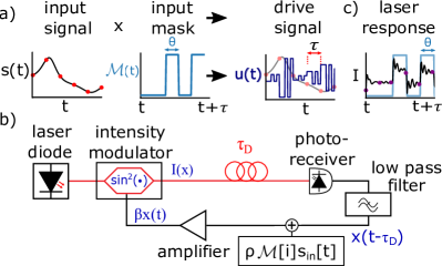
In an opto-electronic RC, illustrated in Fig. 1b, the output of a fiber-coupled continuous wave laser is sent through an intensity modulator, which provides a sinusoidal nonlinearity. The light that is transmitted through the modulator travels through a fiber delay line before being detected by a photoreceiver. The electrical signal from the photoreceiver is combined with the input signal, amplified, and applied to the RF port of the intensity modulator, completing the feedback loop. This opto-electronic feedback loop forms a dynamical system that is used as a reservoir, where the “virtual” nodes come from time multiplexing and the space-time interpretation of delay systems Arecchi et al. (1992); Appeltant et al. (2011); Yanchuk and Giacomelli (2017); Hart et al. (2019).

The input signal must be pre-processed in time-multiplexed reservoir systems. The procedure is depicted in Fig. 1a. A periodic input mask $\mathcal{M}(t)$ of period $\tau_{in}$ is applied to the sampled input data (red dots) to form the drive signal (dark blue); $\tau_{in}$ does not have to be equal to the delay time $\tau_{d}$ Stelzer et al. (2020); Hülser et al. (2022), though here we choose $\tau_{in}=\tau_{d}$, as was done in Refs. Carroll (2021a); Van der Sande, Brunner, and Soriano (2017); Larger et al. (2012); Sugano, Kanno, and Uchida (2019); Harkhoe et al. (2020); Appeltant et al. (2011); Larger et al. (2017); Soriano et al. (2013); Dai and Chembo (2021). The input mask is analogous to $\mathbf{W^{in}}$ in that it provides a different weighting of the input signal to each time-multiplexed node. Indeed, any $\mathbf{W^{in}}$ can be represented by the input mask $\mathcal{M}(t)$ by choosing $\mathcal{M}(t)=\mathbf{W^{in}_{k}}$ with $k=\mod(\lfloor t/\theta\rfloor,M)$. When one period of the mask is complete, the mask is then applied to the next value of the sampled input signal. Therefore, the reservoir updates at a rate of one input sample per unit $\tau_{in}$. As depicted in Fig. 1a, the input mask is piece-wise constant with duration $\theta$, referred to as the node time. In this work 40% of the mask values are chosen randomly from the uniform distribution between -1 and +1, and the remaining elements are set to zero. We found this type of mask to give the best results, as discussed in Section IV.1.

The photoreceiver output voltage is detected and sampled at a rate $1/\theta$, as depicted in Fig. 1c, to obtain the reservoir node states. The voltage is shown as a black line, with purple dots indicating the sampled values used as the reservoir output node states.

The opto-electronic RC can be modeled by the following delay differential equation Larger et al. (2012):

$$\tau_{L}\dot{v}(t)=-v(t)+\beta\sin^{2}\bigg{(}v(t-\tau_{d})+\phi+\rho\mathcal{M}(t)s(t)\bigg{)},$$ (7)

where $v$ is proportional to the voltage applied to the intensity modulator, $\tau_{L}=4\theta$ is the low-pass filter time constant, $\beta=0.8$ is the round trip gain, $\tau_{d}=M\theta$ is the round trip delay time, and $\phi=0.2$ is the modulator DC bias phase. The system is driven by $\rho\mathcal{M}(t)s(t)$, where $\rho=0.4$ is a scale factor, and $s(t)$ is the continuous-time input signal. $s(t)$ is obtained from the discrete-time, sampled input signal $s_{d}[k]$ by $s(t)=s_{d}[\lfloor t/\tau_{in}\rfloor]$. In this work, $\theta=40$, and Eq. 4 is integrated using Heun’s method with a time step of 1.

IV.1 Optimizing the Input Mask

An important question for opto-electronic reservoir computer design is how to choose the input mask. In this section, we investigate this question. It seems likely that driving all the virtual nodes of the reservoir with the input signal could decrease the diversity of the reservoir response; we can quantify this diversity by varying the fraction of virtual nodes that are driven and measuring the resulting entropy of the reservoir. We find that there is an optimal value of $f_{W}$, in this case 40%, that results from a tradeoff between entropy and covariance rank.

IV.1.1 Estimating Entropy

Measuring entropy requires a partitioning of the dynamical system. Reference Xiong, Faes, and Ivanov (2017) lists a number of ways to do this partitioning, although different partitions can give different results for the entropy. It was found that the permutation entropy method Bandt and Pompe (2002) avoided this coarse graining problem because it creates partitions based on the time ordering of the signals. Each individual node time series $\chi_{i}(t)$ was divided into windows of 4 points, and the points within the window were sorted to establish their order; for example, if the points within a window were 0.1, 0.3, -0.1 0.2, the ordering would be 2,4,1,3. Each possible ordering of points in a signal $\chi_{i}(t)$ represented a symbol $\psi_{i}(t)$.

The method of Bandt and Pompe (2002) was adapted for a reservoir computer in Carroll (2021b). At each time step $t$, the individual node signals were combined into a reservoir computer symbol $\Lambda(t)=[\psi_{1}(t),\psi_{2}(t),\ldots\psi_{M}(t)]$. With $M=100$ nodes there were potentially a huge number of possible symbols, but the nodes were all driven by a common drive signal, so only a tiny fraction of the symbol space was actually occupied, on the order of tens of symbols for the entire reservoir computer.

If $K$ total symbols were observed for the reservoir computer for the entire time series, then the reservoir computer entropy was

$$H=-\sum\limits_{k=1}^{K}{p\left({{\Lambda_{k}}}\right)\log\left({p\left({{\Lambda_{k}}}\right)}\right)}$$ (8)

where $p(\Lambda_{k})$ is the probability of the $k^{th}$ symbol.

IV.1.2 Entropy vs. Error

For this simulation, the elements of the input mask ${\bf W}^{in}$ were chosen from a random distribution between -1 and 1, but only a fraction $f_{W}$ of the elements were nonzero. For each value of $f_{W}$, 20 realizations of ${\bf W}^{in}$ were created and the numbers that are plotted are the average from these 20 realizations.

Figure 2 shows the entropy $H$ as a function of the input fraction $f_{W}$ when the reservoir was driven with the Lorenz or the Rössler $x$ signal.

Figure 2: The top plot shows the entropy $H$ of the optoelectronic reservoir driven by the Lorenz or the Rössler $x$ signal as the fraction of nonzero entries in the input mask $f_{W}$ varied. The bottom plot shows the covariance rank $\Gamma$ of the reservoir with the two different input signals

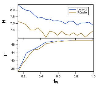
Decreasing the fraction of virtual nodes directly connected to the input signal increases the entropy of the optoelectronic reservoir. Figure 2 also shows the covariance rank of the reservoir driven by the two different input signals.

Figure 3: Observer and prediction testing errors for the optoelectronic reservoir driven by the Lorenz $x$ signal as the fraction of nonzero input mask elements $f_{W}$ varies.

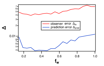
Figure 3 shows that the observer and prediction testing errors both go through a minimum as $f_{W}$ varies. Figure 2 explains the reason for this minimum; as $f_{W}$ gets smaller the reservoir entropy $H$ gets larger, and larger entropy should lead to smaller fitting errors, but the reservoir covariance rank $\Gamma$ gets smaller. Smaller covariance rank should lead to larger fitting errors, so the two effects lead to a minimum in the testing and prediction errors near $f_{W}=0.4$.

Figure 4: Comparison of testing NRMSE for the opto-electronic reservoir computer using RRQR-optimized time-shifts and randomly selected time-shifts as a function of $M_{red}$ for the Lorenz tasks with 10 nodes and $\tau_{max}=10$. (a) One-step prediction. (b) Observer task.

IV.2 Results

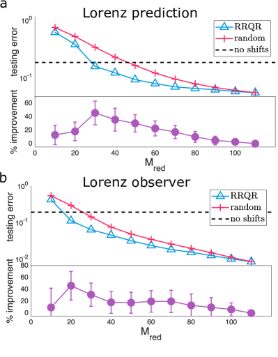
We investigated the effectiveness of the RRQR time-shift rank-optimization described in Section III on an opto-electronic RC with $M=10$ nodes performing the prediction and observer tasks on the Lorenz and Rössler chaotic systems. The testing NRMSE obtained using the best $M_{red}$ node/time-shift combinations are shown as blue triangles in Fig. 4 (Lorenz) and Fig. 5 (Rössler). These results are averaged over 20 different, randomly selected input masks.

For comparison, we show the NRMSE obtained using $M_{red}$ randomly selected columns of $\mathbf{\Omega^{(2)}}$ as red crosses in Figs. 4 and 5. This NRMSE is averaged over 20 different, randomly generated input masks and 20 different, randomly selected node/time-shift combinations. We also show the NRMSE obtained using the non-time-shifted reservoir ($\mathbf{\Omega}$) as a black dotted line.

In all cases, the accuracy improves as $M_{red}$ increases. This is expected, since having a larger state matrix allows for the possibility of a larger state matrix rank. However, the random and rank-optimal state matrices have the same state matrix size for a given $M_{red}$, yet the rank-optimal state matrix generally provides better performance, implying that choosing the correct time-shifts can result in a significant improvement in performance.

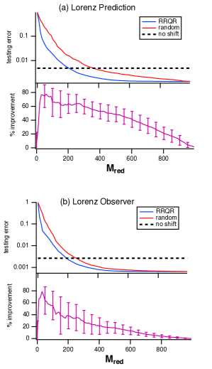
For the Lorenz system (Fig. 4), we find that the testing error using rank-optimal node/time-shift combinations is always better than randomly selected combinations. To quantify this, we compute the percent improvement

$$\mathrm{\%\;improvement}=100\times\frac{\Delta_{test}^{rand}-\Delta_{test}^{RRQR}}{\Delta_{test}^{rand}},$$ (9)

where $\Delta_{test}^{RRQR}$ and $\Delta_{test}^{rand}$ are the testing NRMSE for the rank-optimal and randomly selected node/time-shift combinations, respectively. We see that, for the Lorenz system, the percent improvement provided by the RRQR algorithm is as high as 55% for the prediction task and 68% for the observer task. As expected, as $M_{red}$ approaches $M(\tau_{max}+1),$ the testing errors from the rank-optimal and random selections converge, since in both cases all node/time-shift combinations are being used (i.e., the full $\mathbf{\Omega^{(2)}}$ is used). The error bars for the improvement metric were determined by computing the improvement metric for each reservoir realization, and using the standard deviation of this data set as the error bars. We did not compute error bars for the testing errors because any error bar computation for the testing errors for the randomly chosen time-shifts will confuse variation in performance from reservoir to reservoir with variation in performance due to the different randomly selected time-shifts.

Figure 5: Comparison of testing NRMSE for the opto-electronic reservoir computer using RRQR-optimized time-shifts and randomly selected time-shifts as a function of $M_{red}$ for the Rössler tasks with 10 nodes and $\tau_{max}=10$. (a) One-step prediction. (b) Observer task.

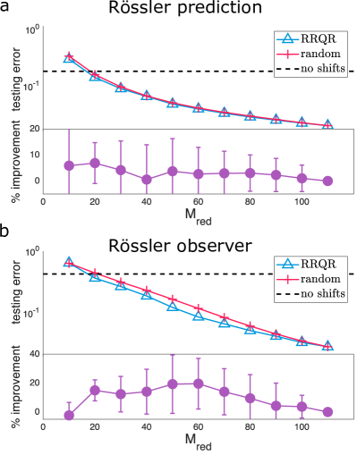
For the Rössler system (Fig. 5), we similarly find that the testing error using rank-optimal node/time-shift combinations is nearly always better than randomly selected combinations, but the improvement is more modest, especially for the prediction task. We suspect that this performance reduction is due to the long correlation time of the Rössler system, which means that the time-shifted signals are not so different from one another. This is supported by Fig. 2, in which the entropy statistic shows that there is less diversity among the different columns when the reservoir is driven by the Rössler $x$ variable. In this case, one would not expect the particular selection of node/time-shift combinations to make as much difference as for the Lorenz system which has a much shorter correlation time and for which the reservoir displays a larger entropy.

Figure 6: Comparison of testing NRMSE for the leaky $tanh$ reservoir computer using RRQR-optimized time shifts and randomly selected time shifts as a function of $M_{red}$ for the Lorenz tasks with 100 nodes and $\tau_{max}=10$. (a) One step prediction of the Lorenz $x$ variable. (b) Observer task of the Lorenz $z$ variable based on the Lorenz $x$ variable.

It is important to note that the RRQR algorithm selects the most linearly independent columns of the full reservoir matrix $\mathbf{\Omega^{(2)}}$; it does not provide an optimal $\tau_{max}$. This explains why both the rank-optimized and randomly-selected time-shifts perform worse than the unshifted reservoir for $M_{red}=10$: The time-shifts retained include large shifts, which, while more linearly independent, are less correlated with the current system state than the unshifted nodes. For small $M_{red}$, the RRQR method performs better than the unshifted reservoir only for small $\tau_{max}$ (not shown).

We have tested our RRQR method on larger opto-electronic RCs (up to $M=800$) and using different $\tau_{max}$, and found similar results.

V Time-shift rank-optimization for the Leaky Tanh Reservoir

In the previous section, we showed that rank-optimization significantly improves the performance of an optoelectronic reservoir. In order to demonstrate the generality of this technique, in this section we show that the rank-optimization is also useful for a leaky $tanh$ reservoir Jaeger (2001). This reservoir computer is described by

$$\begin{split}{\bf{\chi}}[{n+1}]=&\left(1-\alpha\right)\mathbf{\chi}[n]+\\ &\alpha\tanh\left({{\bf{A}\chi[n]}+\mathbf{W}^{in}s[n]}+1\right)\end{split}$$ (10)

For these simulations, half the elements of ${\bf A}$ were chosen from a uniform random distribution between -1 and 1 while the others were zero, and then the the diagonal of ${\bf A}$ was set to zero. ${\bf A}$ was then renormalized so its spectral radius was 0.5. The parameter $\alpha=0.35$ was found to minimize the testing error. The signals $\chi_{j}[i]$ were arranged in a matrix $\Omega$ in the same manner as in Eq. (2) and the reservoir computer was used to fit training and testing signals as in Section II, with the testing error being calculated as in Eq. (3). As in the optoelectronic system, optimization revealed that the best testing error was found when 40% of the elements of ${\bf W^{in}}$ were nonzero.

V.1 Results

The testing NRMSE using the rank-optimal $M_{red}$ node/time shift combinations for the leaky $tanh$ reservoir and the Lorenz system is shown in Fig. 6 and for the Rössler system in Fig. 7.

Figure 7: Comparison of testing NRMSE for the leaky $tanh$ reservoir computer using RRQR-optimized time shifts and randomly selected time shifts as a function of $M_{red}$ for the Rössler tasks with 100 nodes and $\tau_{max}=10$. (a) One step prediction of the Rössler $x$ variable. (b) Observer task of the Rössler $z$ variable based on the Rössler $x$ variable.

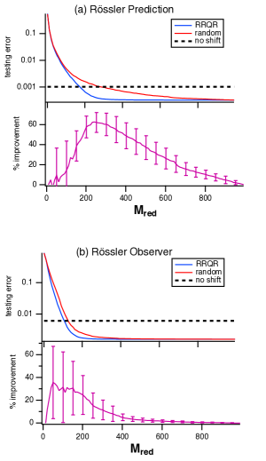
The improvement in testing error in the leaky $tanh$ reservoir computer gained by using rank-optimal time shift/node combinations is even larger than in the opto-electronic reservoir computer. The opto-electronic system does have more symmetry because the coupling between virtual nodes is a one way ring Hart et al. (2019), while the coupling in the leaky $tanh$ system is random. Similarly to the opto-electronic system, the improvement is larger for the Lorenz tasks than for the Rössler tasks.

VI Conclusions

We have proposed a technique for selecting the rank-optimal combination of time-shifts for a reservoir computer based on a rank-revealing QR algorithm. We demonstrated that a reservoir computer with our rank-optimized time-shifts displays significantly higher accuracy than with random time-shifts. We have verified that this technique is general by demonstrating improved performance on both analog and digital reservoir computers. Our technique is task-independent and does not rely on a model of the reservoir computer, so it can be straightforwardly applied to both digital and analog reservoir computer implementations.

Author Declarations: The authors have no conflicts of interest to disclose.

Data Availability: The data that support the findings of this study are available from the corresponding author upon reasonable request.

Acknowledgements: JDH and TLC acknowledge support from the Naval Research Laboratory’s Basic Research Program and from the Office of the Secretary of Defense through the Applied Research for Advancement of S&T Priorities (ARAP) program under the Neuropipe project.

References

- Maass, Natschläger, and Markram (2002) W. Maass, T. Natschläger, and H. Markram, “Real-time computing without stable states: A new framework for neural computation based on perturbations,” Neural Comput. 14, 2531–2560 (2002).
- Jaeger and Haas (2004) H. Jaeger and H. Haas, “Harnessing nonlinearity: Predicting chaotic systems and saving energy in wireless communication,” Science 304, 78–80 (2004).
- Pathak et al. (2018) J. Pathak, B. Hunt, M. Girvan, Z. Lu, and E. Ott, “Model-free prediction of large spatiotemporally chaotic systems from data: A reservoir computing approach,” Phys. Rev. Lett. 120, 024102 (2018).
- Gauthier and Fischer (2021) D. J. Gauthier and I. Fischer, “Predicting hidden structure in dynamical systems,” Nat. Mach. Intell. 3, 281–282 (2021).
- Canaday, Pomerance, and Gauthier (2021) D. Canaday, A. Pomerance, and D. J. Gauthier, “Model-free control of dynamical systems with deep reservoir computing,” J. of Phys.: Complexity 2, 035025 (2021).
- Del Frate, Shirin, and Sorrentino (2021) E. Del Frate, A. Shirin, and F. Sorrentino, “Reservoir computing with random and optimized time-shifts,” Chaos 31, 121103 (2021).
- Carroll and Hart (2022) T. L. Carroll and J. D. Hart, “Time shifts to reduce the size of reservoir computers,” Chaos 32, 083122 (2022).
- Tanaka et al. (2019) G. Tanaka, T. Yamane, J. B. Héroux, R. Nakane, N. Kanazawa, S. Takeda, H. Numata, D. Nakano, and A. Hirose, “Recent advances in physical reservoir computing: A review,” Neural Netw. 115, 100–123 (2019).
- Van der Sande, Brunner, and Soriano (2017) G. Van der Sande, D. Brunner, and M. C. Soriano, “Advances in photonic reservoir computing,” Nanophotonics 6, 561–576 (2017).
- Du et al. (2017) C. Du, F. Cai, M. A. Zidan, W. Ma, S. H. Lee, and W. D. Lu, “Reservoir computing using dynamic memristors for temporal information processing,” Nat. Commun. 8, 1–10 (2017).
- Larger et al. (2017) L. Larger, A. Baylón-Fuentes, R. Martinenghi, V. S. Udaltsov, Y. K. Chembo, and M. Jacquot, “High-speed photonic reservoir computing using a time-delay-based architecture: Million words per second classification,” Phys. Rev. X 7, 011015 (2017).
- Sugano, Kanno, and Uchida (2019) C. Sugano, K. Kanno, and A. Uchida, “Reservoir computing using multiple lasers with feedback on a photonic integrated circuit,” IEEE J. Sel. Top. Quantum Electron. 26, 1–9 (2019).
- Jaurigue et al. (2021) L. Jaurigue, E. Robertson, J. Wolters, and K. Lüdge, “Reservoir computing with delayed input for fast and easy optimisation,” Entropy 23, 1560 (2021).
- Carroll (2021a) T. L. Carroll, “Adding filters to improve reservoir computer performance,” Physica D 416, 132798 (2021a).
- Takano et al. (2018) K. Takano, C. Sugano, M. Inubushi, K. Yoshimura, S. Sunada, K. Kanno, and A. Uchida, “Compact reservoir computing with a photonic integrated circuit,” Opt. Express 26, 29424–29439 (2018).
- Harkhoe et al. (2020) K. Harkhoe, G. Verschaffelt, A. Katumba, P. Bienstman, and G. Van der Sande, “Demonstrating delay-based reservoir computing using a compact photonic integrated chip,” Opt. Express 28, 3086–3096 (2020).
- Sunada and Uchida (2021) S. Sunada and A. Uchida, “Photonic neural field on a silicon chip: large-scale, high-speed neuro-inspired computing and sensing,” Optica 8, 1388–1396 (2021).
- Marquez, Suarez-Vargas, and Shastri (2019) B. A. Marquez, J. Suarez-Vargas, and B. J. Shastri, “Takens-inspired neuromorphic processor: A downsizing tool for random recurrent neural networks via feature extraction,” Phys. Rev. Research 1, 033030 (2019).
- Tikhonov, Arsenin, and John (1977) A. N. Tikhonov, V. I. Arsenin, and F. John, Solutions of ill-posed problems, Vol. 14 (Winston, Washington, 1977).
- Carroll and Pecora (2019) T. L. Carroll and L. M. Pecora, “Network structure effects in reservoir computers,” Chaos 29, 083130 (2019).
- Abdi and Williams (2010) H. Abdi and L. J. Williams, “Principal component analysis,” Wiley Interdiscip. Rev. Comput. Stat. 2, 433–459 (2010).
- Uchida, McAllister, and Roy (2004) A. Uchida, R. McAllister, and R. Roy, “Consistency of nonlinear system response to complex drive signals,” Phys. Rev. Lett. 93, 244102 (2004).
- Chan (1987) T. F. Chan, “Rank revealing qr factorizations,” Linear Algebra Its Appl. 88, 67–82 (1987).
- Stewart (1984) G. Stewart, “Rank degeneracy,” SIAM J. Sci. Statist. Comput. 5, 403–413 (1984).
- Appeltant et al. (2011) L. Appeltant, M. C. Soriano, G. Van der Sande, J. Danckaert, S. Massar, J. Dambre, B. Schrauwen, C. R. Mirasso, and I. Fischer, “Information processing using a single dynamical node as complex system,” Nat. Commun. 2, 1–6 (2011).
- Paquot et al. (2012) Y. Paquot, F. Duport, A. Smerieri, J. Dambre, B. Schrauwen, M. Haelterman, and S. Massar, “Optoelectronic reservoir computing,” Sci. Rep. 2, 1–6 (2012).
- Larger et al. (2012) L. Larger, M. C. Soriano, D. Brunner, L. Appeltant, J. M. Gutiérrez, L. Pesquera, C. R. Mirasso, and I. Fischer, “Photonic information processing beyond turing: an optoelectronic implementation of reservoir computing,” Opt. Express 20, 3241–3249 (2012).
- Soriano et al. (2013) M. C. Soriano, S. Ortín, D. Brunner, L. Larger, C. R. Mirasso, I. Fischer, and L. Pesquera, “Optoelectronic reservoir computing: tackling noise-induced performance degradation,” Opt. Express 21, 12–20 (2013).
- Chembo (2020) Y. K. Chembo, “Machine learning based on reservoir computing with time-delayed optoelectronic and photonic systems,” Chaos 30, 013111 (2020).
- Dai and Chembo (2021) H. Dai and Y. K. Chembo, “Classification of iq-modulated signals based on reservoir computing with narrowband optoelectronic oscillators,” IEEE J. Quantum Electron. 57, 1–8 (2021).
- Antonik et al. (2016) P. Antonik, F. Duport, M. Hermans, A. Smerieri, M. Haelterman, and S. Massar, “Online training of an opto-electronic reservoir computer applied to real-time channel equalization,” IEEE Trans. Neural Netw. Learn. Syst. 28, 2686–2698 (2016).
- Duport et al. (2016) F. Duport, A. Smerieri, A. Akrout, M. Haelterman, and S. Massar, “Virtualization of a photonic reservoir computer,” J. Light. Technol. 34, 2085–2091 (2016).
- Ortín et al. (2015) S. Ortín, M. C. Soriano, L. Pesquera, D. Brunner, D. San-Martín, I. Fischer, C. Mirasso, and J. Gutiérrez, “A unified framework for reservoir computing and extreme learning machines based on a single time-delayed neuron,” Sci. Rep. 5, 1–11 (2015).
- Qin et al. (2017) J. Qin, Q. Zhao, H. Yin, Y. Jin, and C. Liu, “Numerical simulation and experiment on optical packet header recognition utilizing reservoir computing based on optoelectronic feedback,” IEEE Photonics J. 9, 1–11 (2017).
- Arecchi et al. (1992) F. Arecchi, G. Giacomelli, A. Lapucci, and R. Meucci, “Two-dimensional representation of a delayed dynamical system,” Phys. Rev. A 45, R4225 (1992).
- Yanchuk and Giacomelli (2017) S. Yanchuk and G. Giacomelli, “Spatio-temporal phenomena in complex systems with time delays,” J. Phys. A 50, 103001 (2017).
- Hart et al. (2019) J. D. Hart, L. Larger, T. E. Murphy, and R. Roy, “Delayed dynamical systems: Networks, chimeras and reservoir computing,” Phil. Trans. R. Soc. A 377, 20180123 (2019).
- Stelzer et al. (2020) F. Stelzer, A. Röhm, K. Lüdge, and S. Yanchuk, “Performance boost of time-delay reservoir computing by non-resonant clock cycle,” Neural Netw. 124, 158–169 (2020).
- Hülser et al. (2022) T. Hülser, F. Köster, L. Jaurigue, and K. Lüdge, “Role of delay-times in delay-based photonic reservoir computing,” Opt. Mater. Express 12, 1214–1231 (2022).
- Xiong, Faes, and Ivanov (2017) W. Xiong, L. Faes, and P. C. Ivanov, “Entropy measures, entropy estimators, and their performance in quantifying complex dynamics: Effects of artifacts, nonstationarity, and long-range correlations,” Phys. Rev. E 95, 062114 (2017).
- Bandt and Pompe (2002) C. Bandt and B. Pompe, “Permutation entropy: a natural complexity measure for time series,” Phys. Rev. Lett. 88, 174102 (2002).
- Carroll (2021b) T. L. Carroll, “Optimizing reservoir computers for signal classification,” Front. Physiol. 12 (2021b), 10.3389/fphys.2021.685121.
- Jaeger (2001) H. Jaeger, “The echo state approach to analysing and training recurrent neural networks,” German National Research Center for Information Technology GMD Technical Report 148, 34 (2001).