Refining Generative Process with Discriminator Guidance
in Score-based Diffusion Models

Dongjun Kim    Yeongmin Kim    Se Jung Kwon    Wanmo Kang    Il-Chul Moon
Abstract

The proposed method, Discriminator Guidance, aims to improve sample generation of pre-trained diffusion models. The approach introduces a discriminator that gives explicit supervision to a denoising sample path whether it is realistic or not. Unlike GANs, our approach does not require joint training of score and discriminator networks. Instead, we train the discriminator after score training, making discriminator training stable and fast to converge. In sample generation, we add an auxiliary term to the pre-trained score to deceive the discriminator. This term corrects the model score to the data score at the optimal discriminator, which implies that the discriminator helps better score estimation in a complementary way. Using our algorithm, we achive state-of-the-art results on ImageNet 256x256 with FID 1.83 and recall 0.64, similar to the validation data’s FID (1.68) and recall (0.66). We release the code at https://github.com/alsdudrla10/DG.

Machine Learning, ICML

Refer to caption
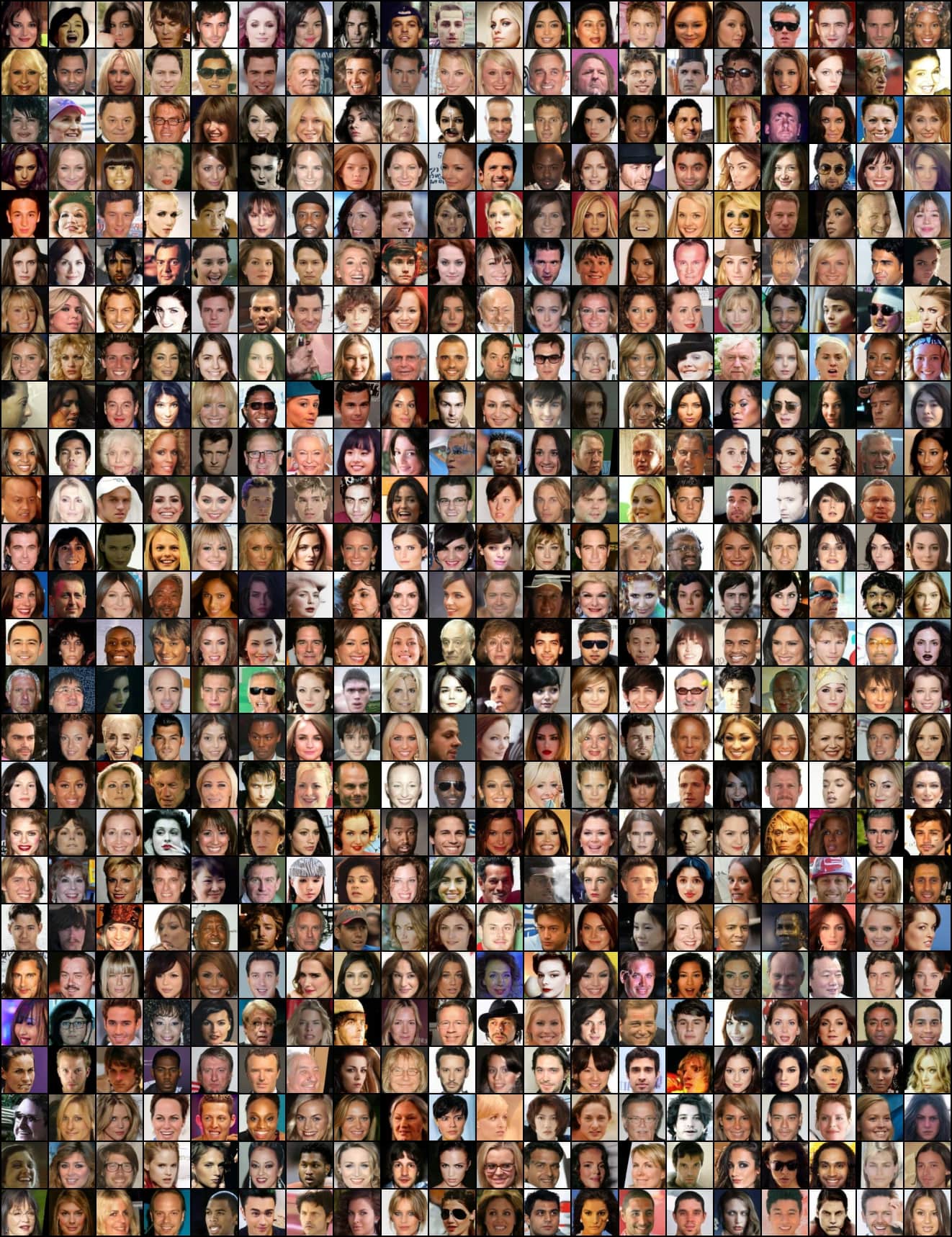
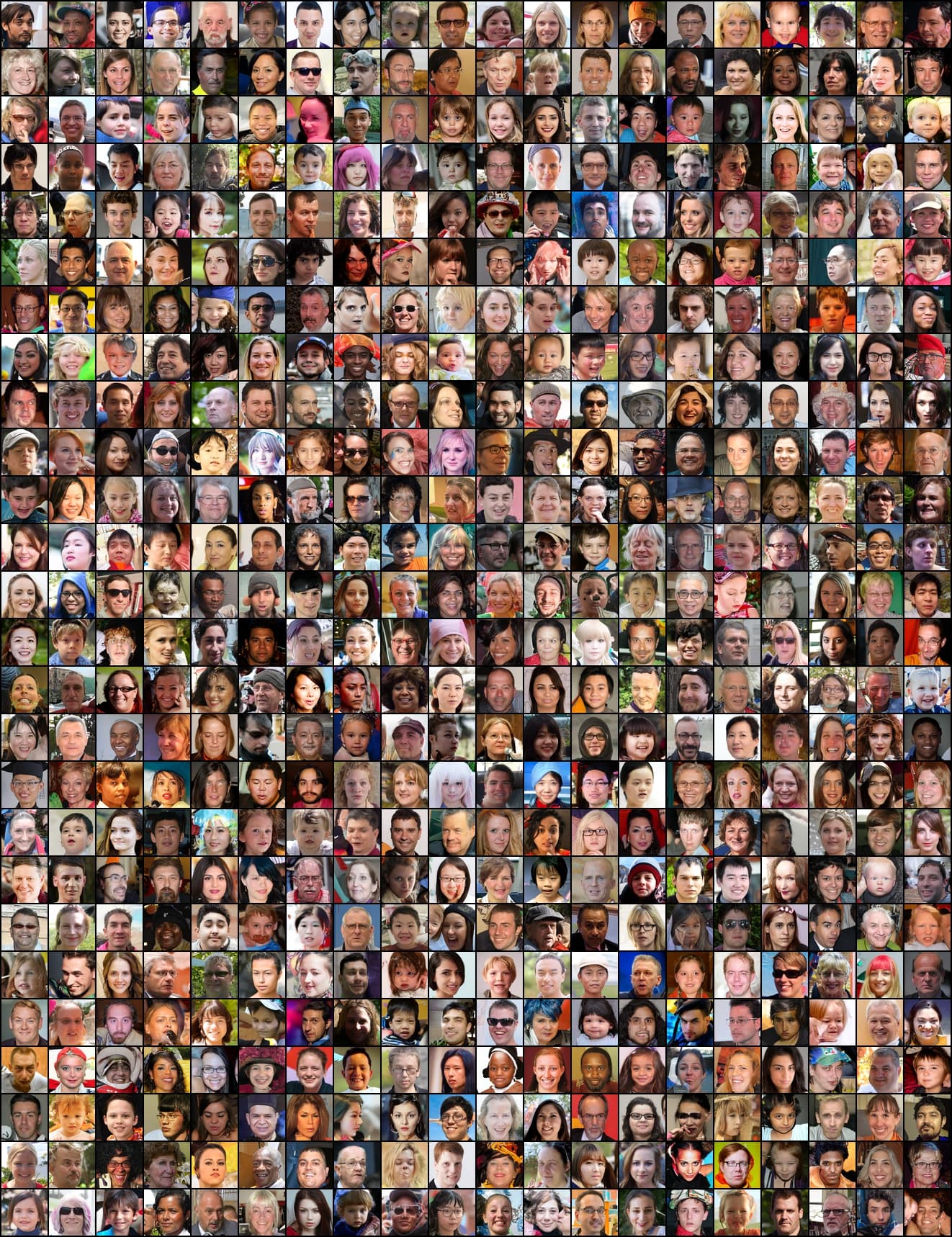
Figure 1: Comparison of the denoising processes. Discriminator Guidance adjusts the score function by estimating the gap 𝐜ϕfragmentscbold-italic-ϕ\mathbf{c}_{\bm{\phi}} between the predicted model score and the true data score. As a result, the sample generated using Discriminator Guidance is indistinguishable from real data according to the discriminator.

1 Introduction

The diffusion model has recently been highlighted for its success in image generation (Dhariwal & Nichol, 2021; Ho et al., 2022a; Karras et al., 2022; Song et al., 2020b), video generation (Singer et al., 2022; Ho et al., 2022b; Voleti et al., 2022), and text-to-image generation (Rombach et al., 2022; Ramesh et al., 2022; Saharia et al., 2022). The State-Of-The-Art (SOTA) models perform human-level generation, but there is still much more room to be investigated for a deep understanding on diffusion models.

Refer to caption
(a) ADM (Dhariwal & Nichol, 2021)
Refer to caption
(b) ADM-G (Dhariwal & Nichol, 2021)
Refer to caption
(c) ADM-G++ (Ours)
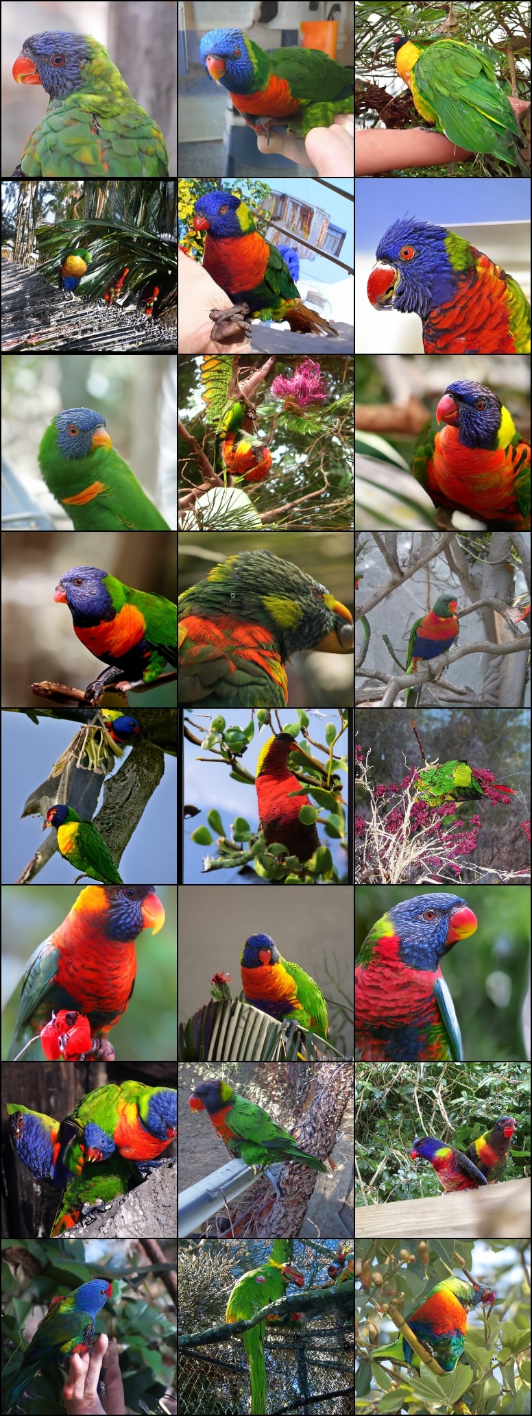
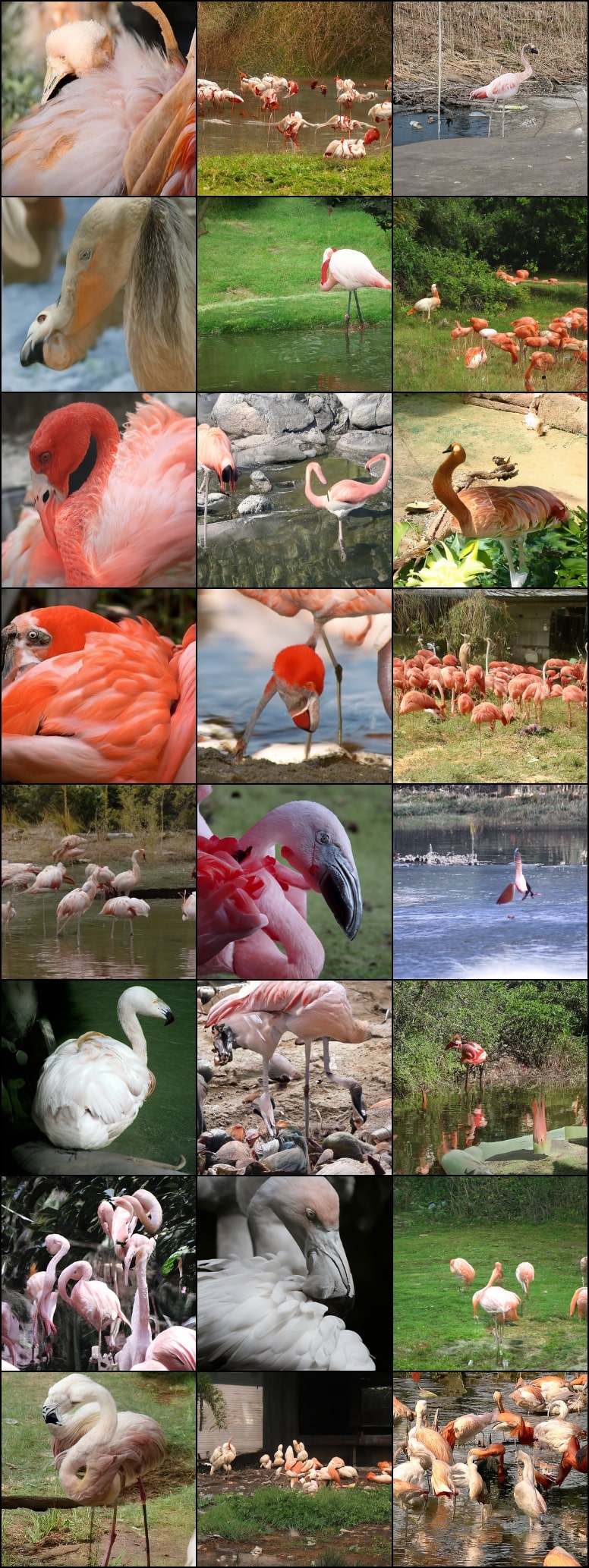
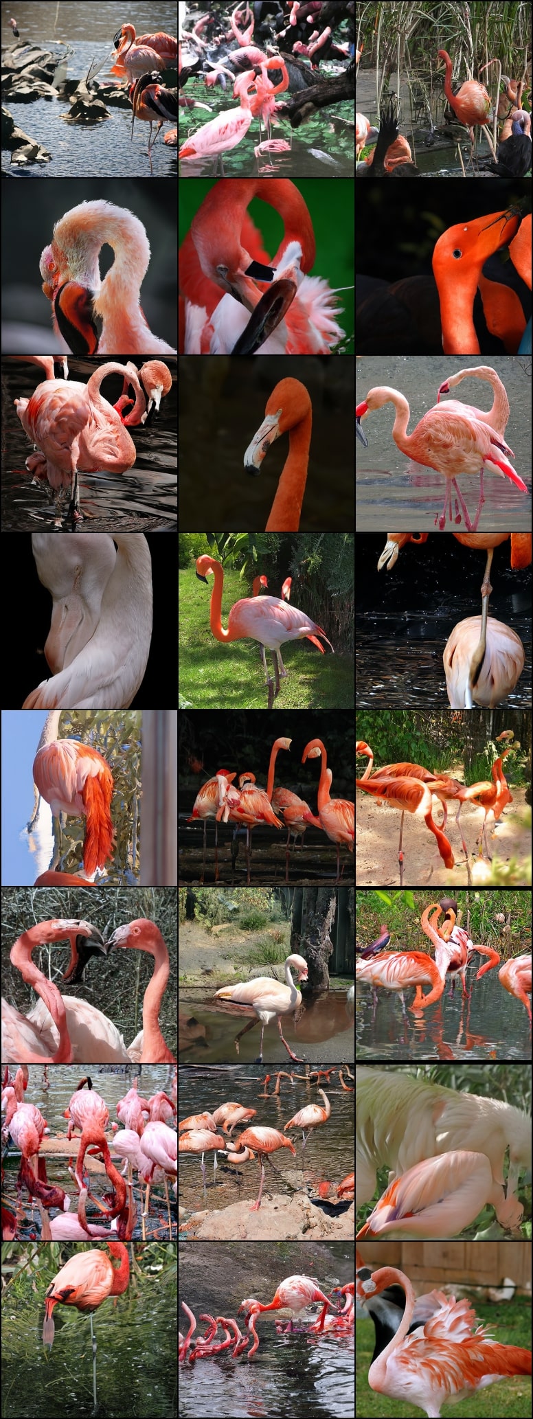
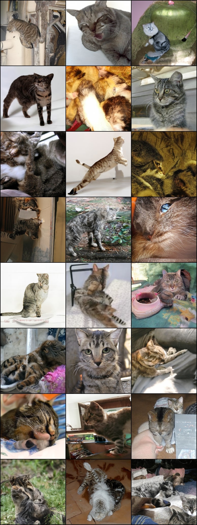
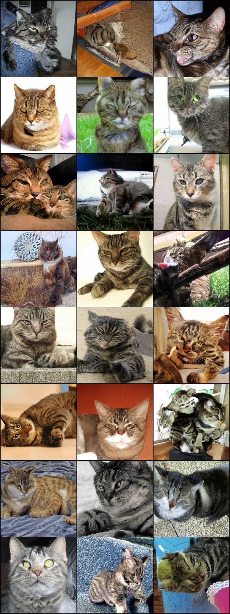
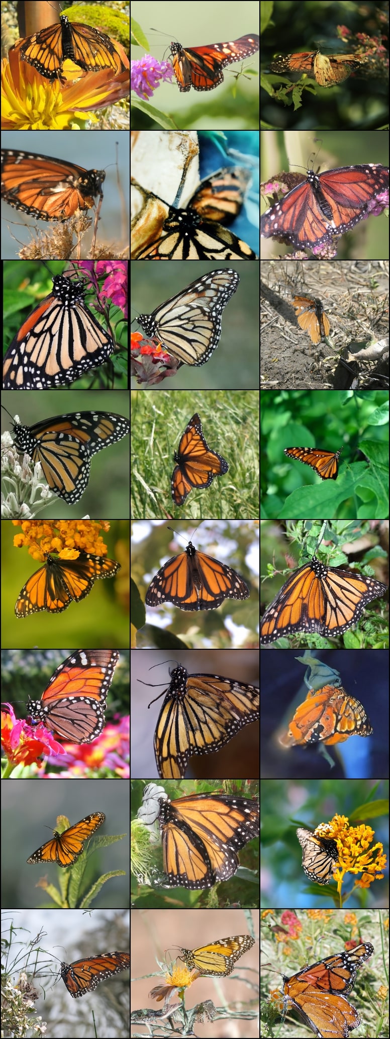
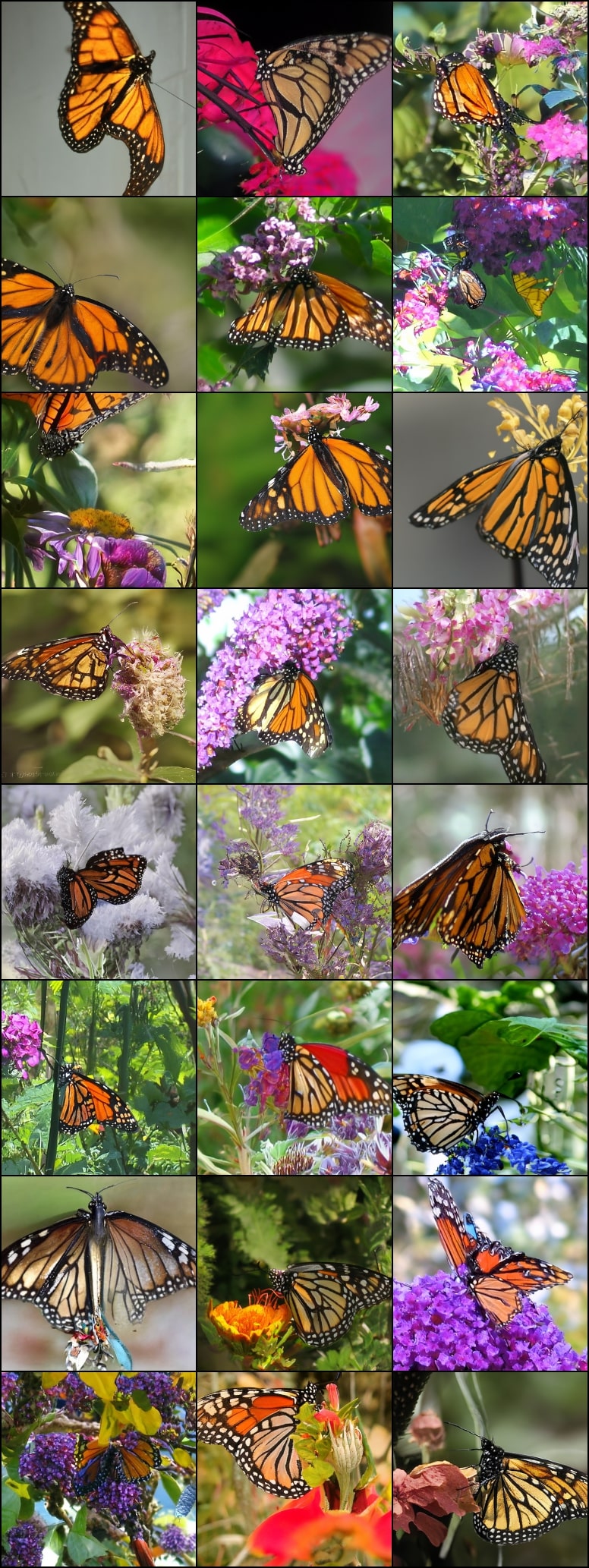
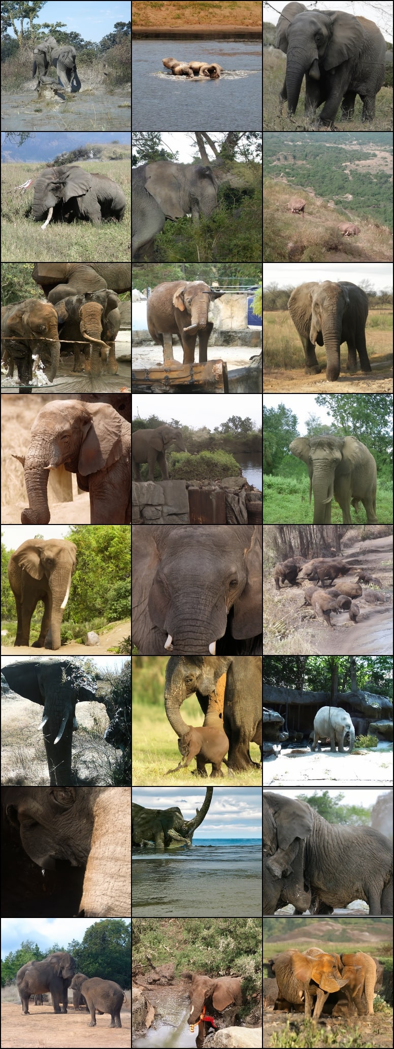
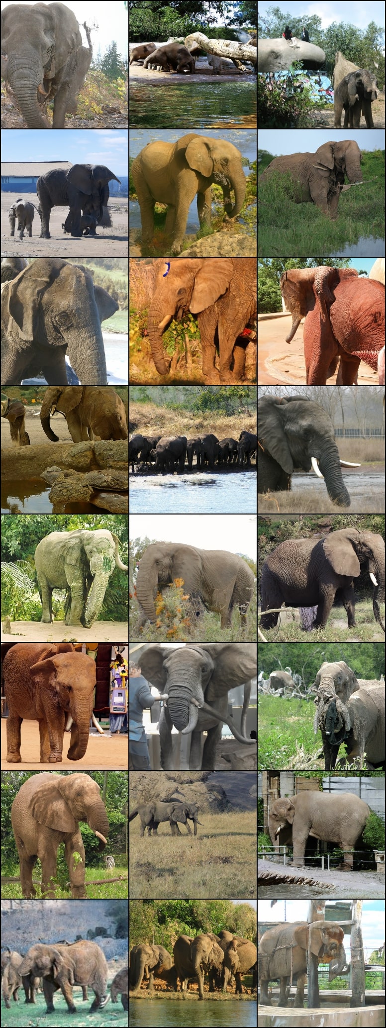
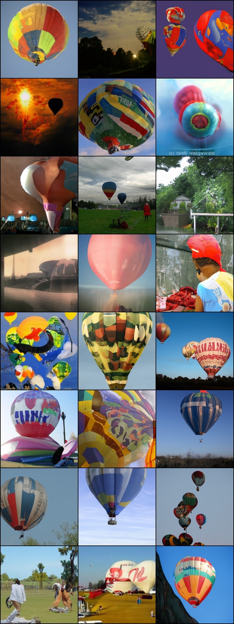
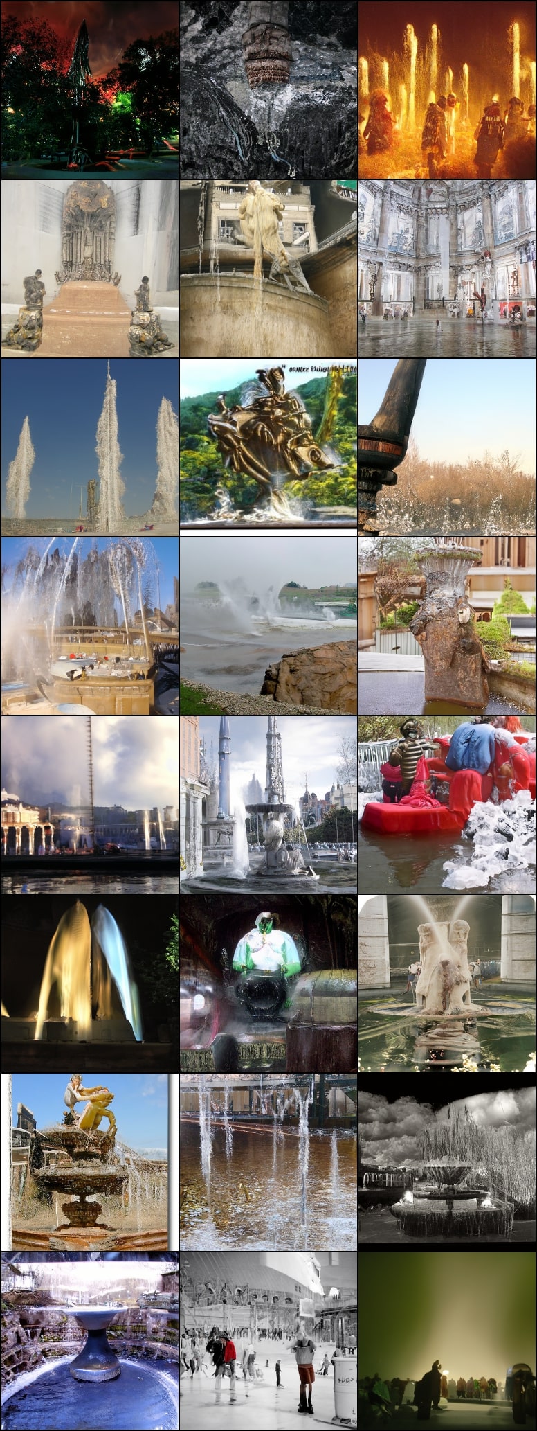
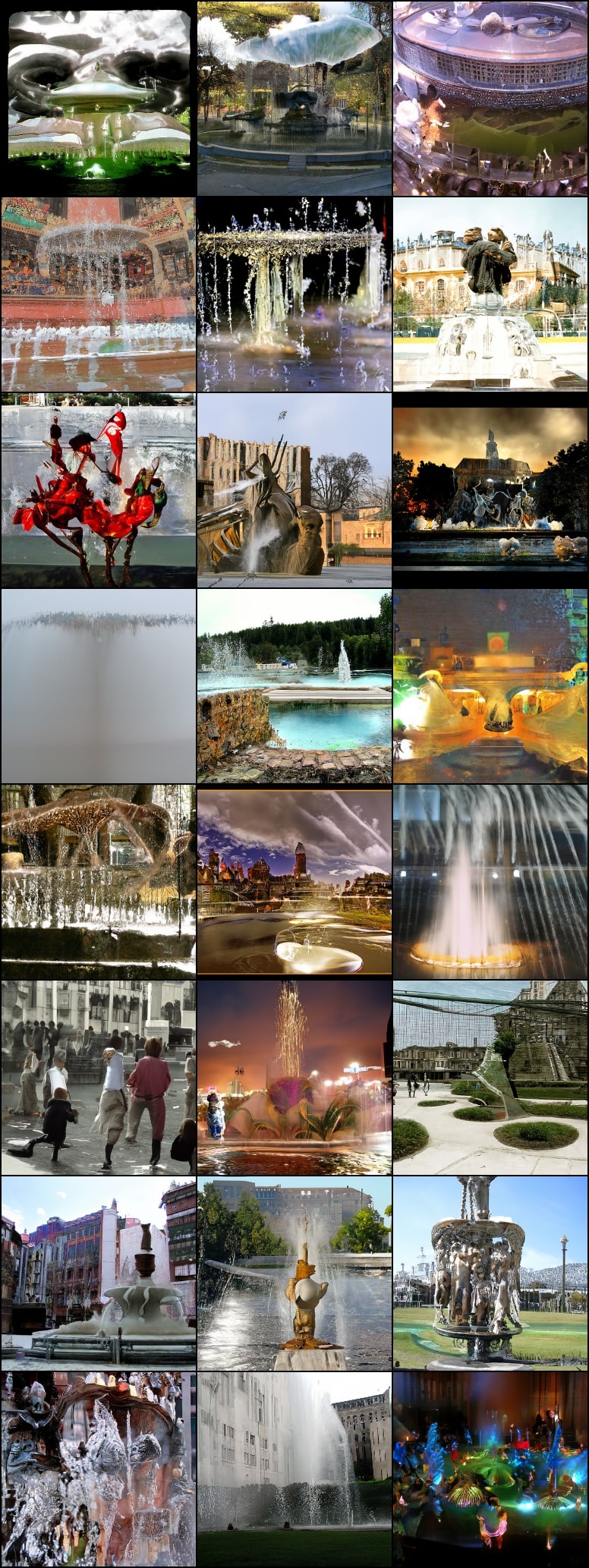
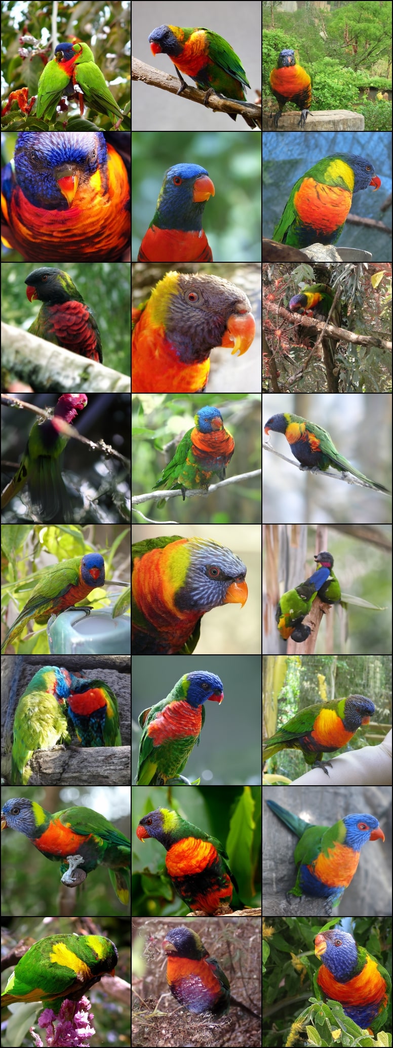
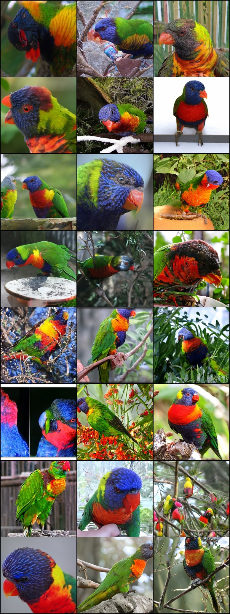
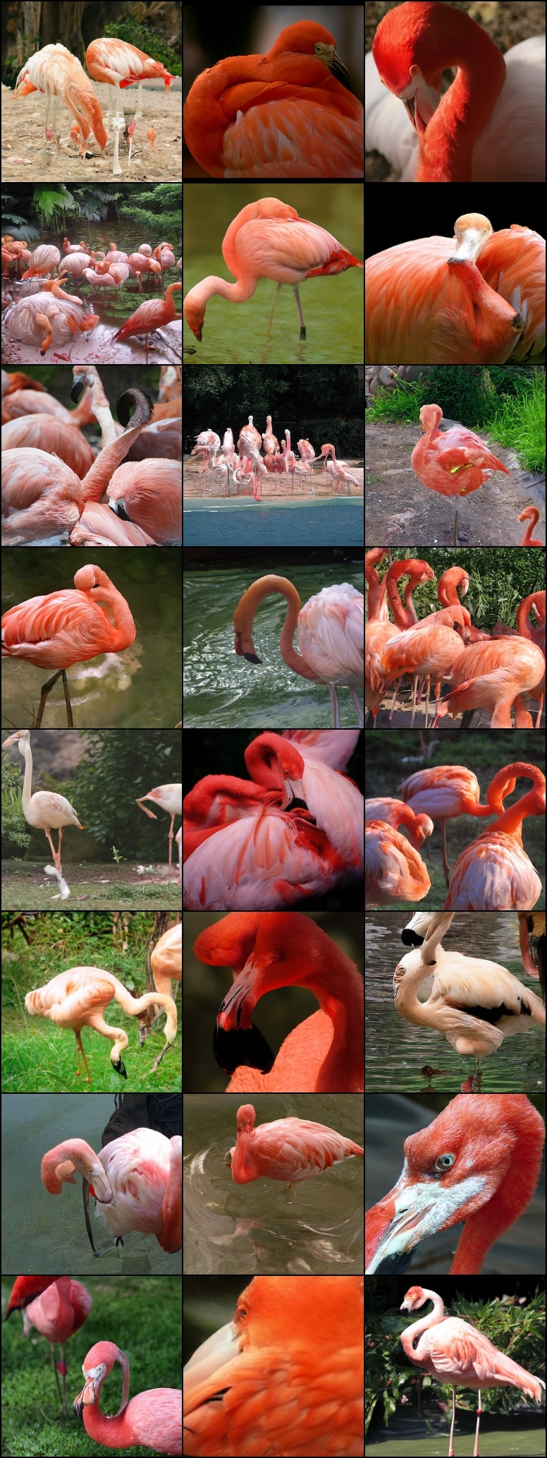
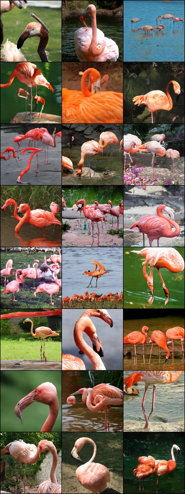
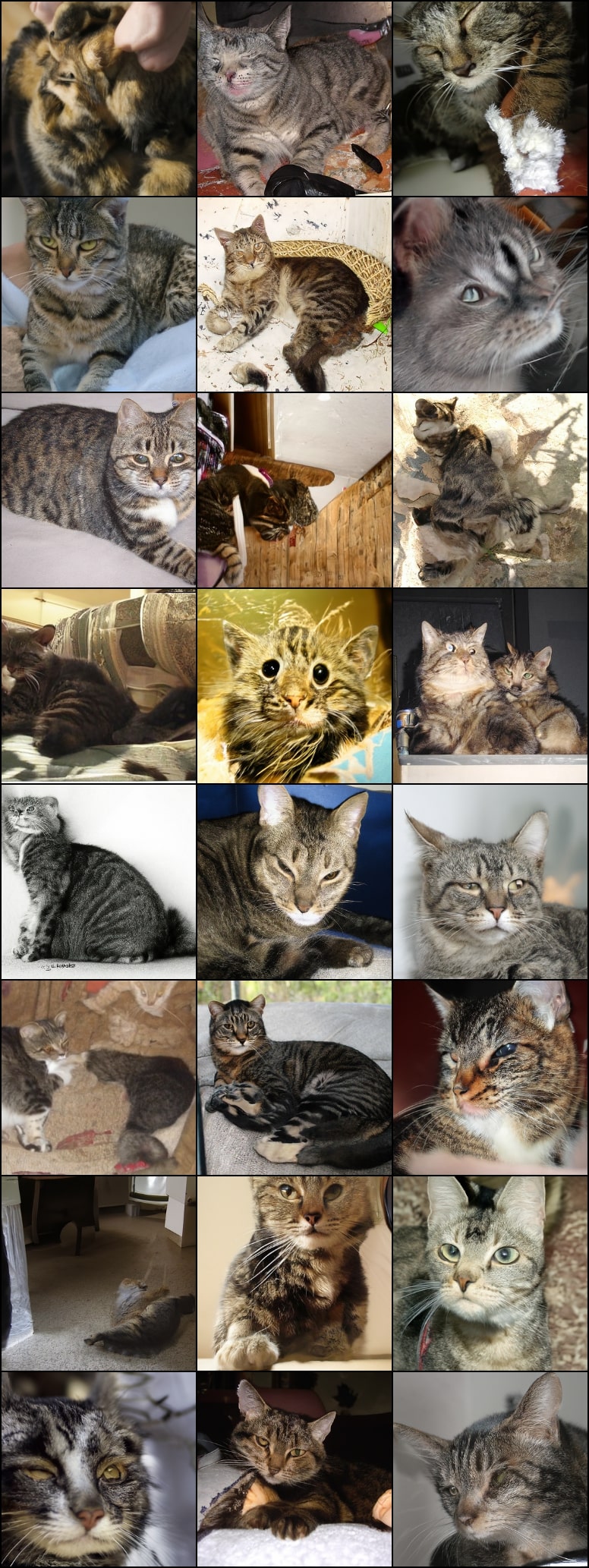
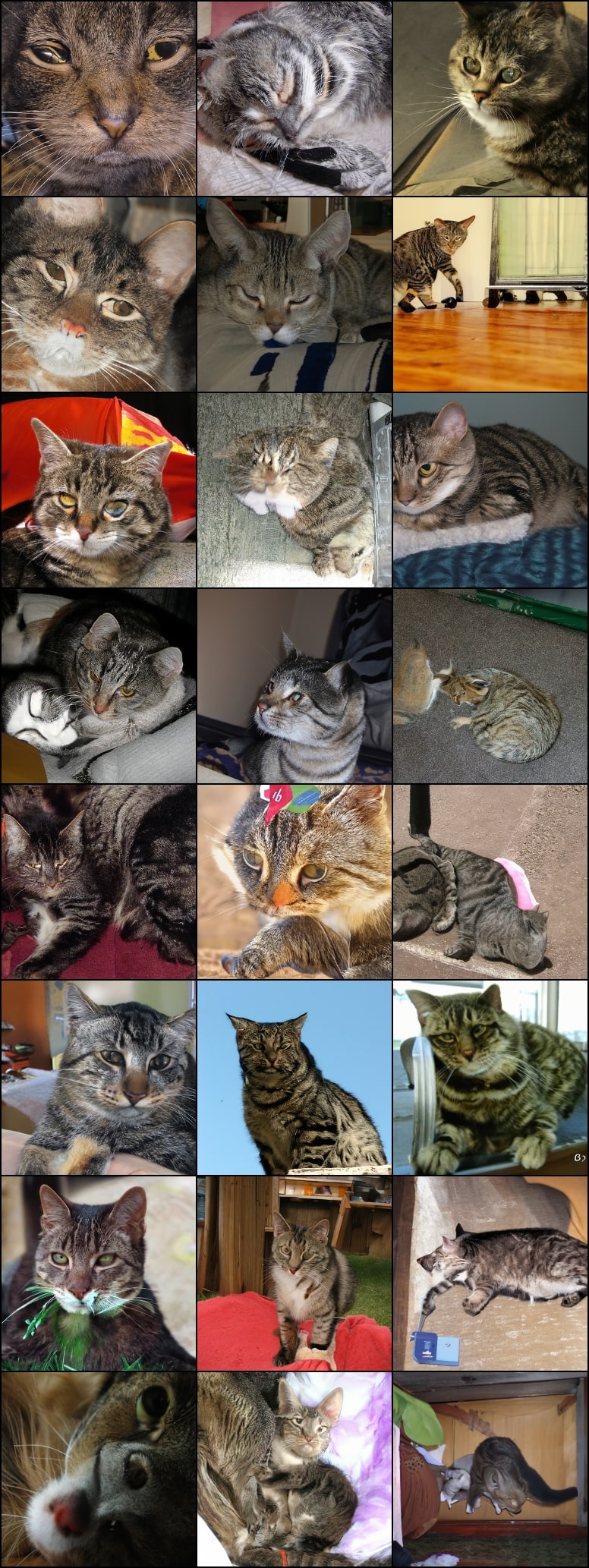
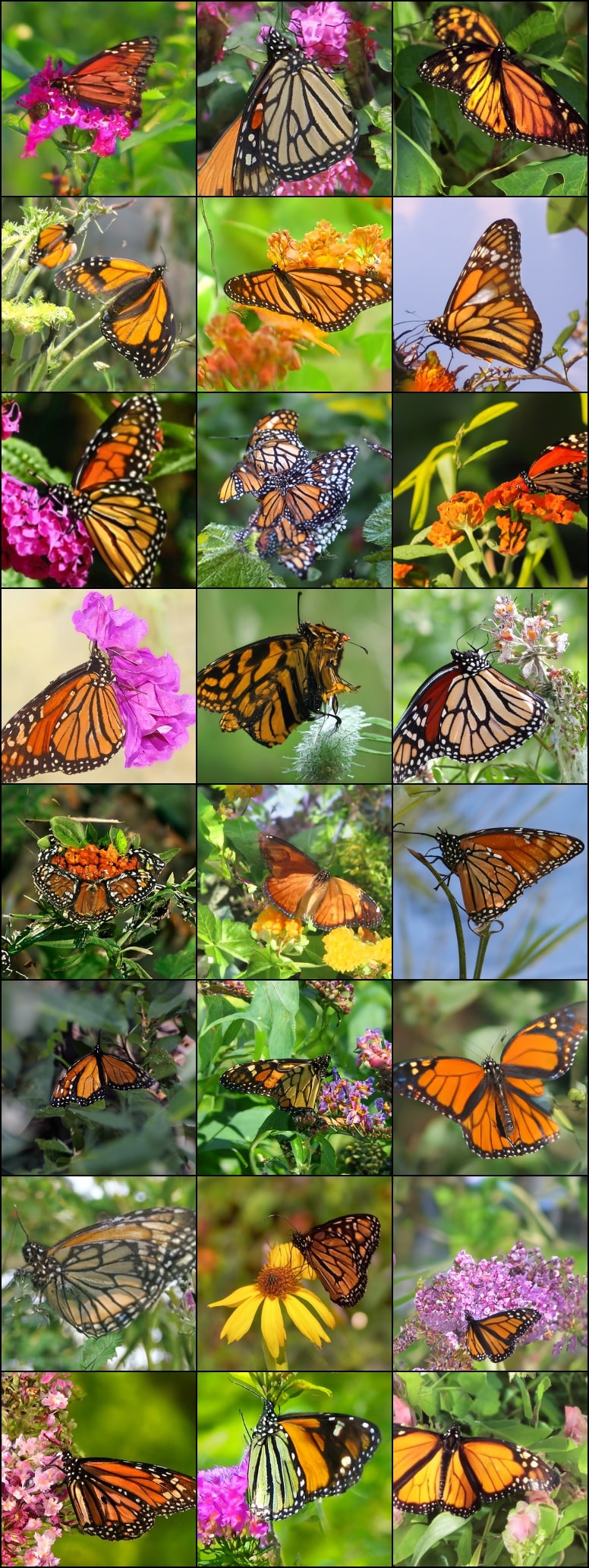
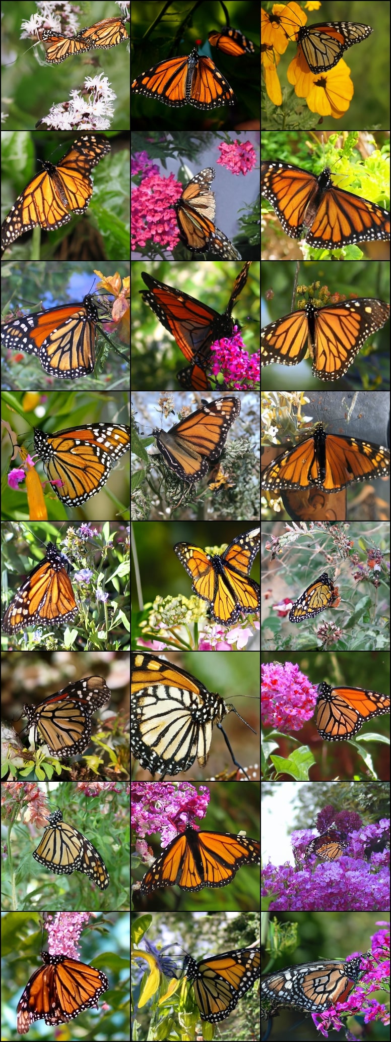
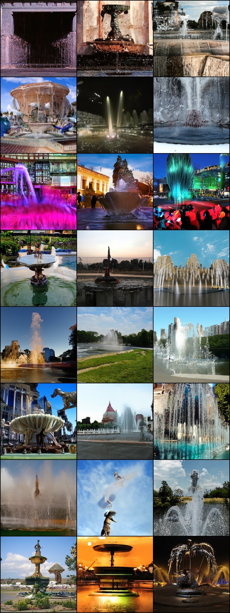
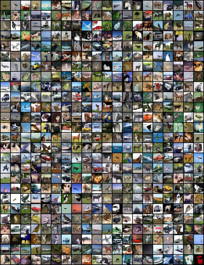
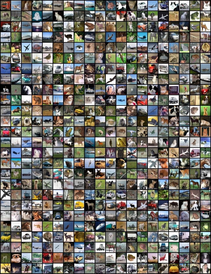
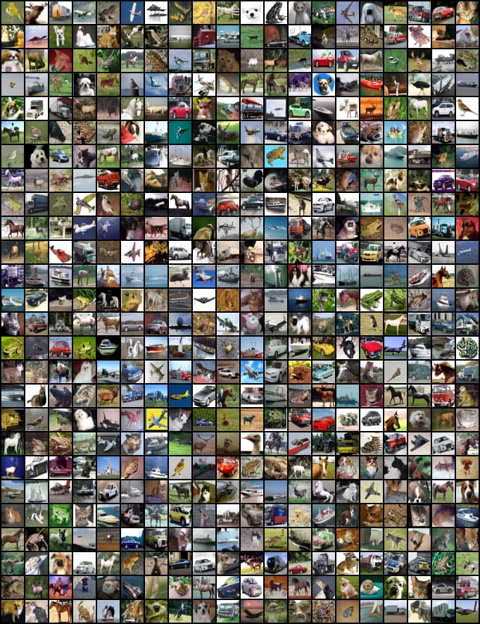
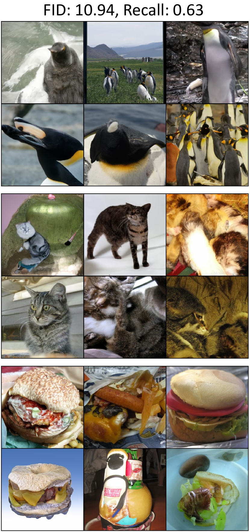
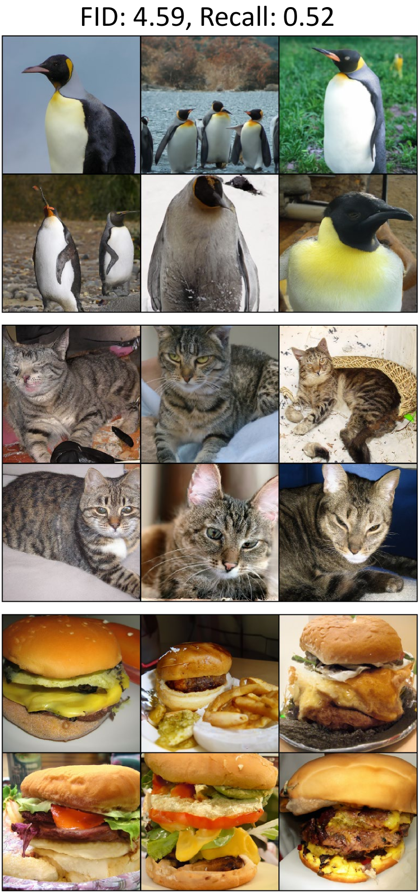
Figure 2: Samples from ImageNet 256x256 on (a) ADM, (b) ADM with Classifier Guidance. Classifier Guidance generates high-fidelity but mode degenerated samples. (c) Classifier Guidance combined with Discriminator Guidance improves both sample quality and intra-class diversity. See Appendix D.4 for uncurated samples of SOTA models.

The generative model community widely uses well-trained score models (Dhariwal & Nichol, 2021; Rombach et al., 2022) in downstream tasks (Meng et al., 2021; Kawar et al., 2022; Su et al., 2022; Kim et al., ). This is partially because training a new score model from scratch can be computationally expensive. However, as the demand for reusing pre-trained models increases, there are only a few research efforts that focus on improving sample quality with a pre-trained score model.

To avoid issues such as overfitting (Nichol & Dhariwal, 2021) or memorization (Carlini et al., 2023) that may arise from further score training (Figure 25), our approach keeps the pre-trained score model fixed and introduces a new component that provides a supervision during sample generation. Specifically, we propose using a discriminator as an auxiliary degree of freedom to the pre-trained model. This discriminator classifies real and generated data at all noise scales, providing direct feedback to the sample denoising process, indicating whether the sample path is realistic or not. We achieve this by adding a correction term to the model score, constructed by the discriminator, which steers the sample path towards more realistic regions (Figure 1). This term is designed to adjust the model score to match the data score at the optimal discriminator (Theorem 1), allowing our approach to find a realistic sample path by adjusting the model score. In experiments, we achieve new SOTA performances on image datasets such as CIFAR-10, CelebA/FFHQ 64x64, and ImageNet 256x256. As discriminator training is a minimization problem that is stable and fast to converge (Figure 3), such a significant gain can be achieved with a cheap budget (Table 6). We summarize the contributions as follows.

  • We propose a new generative process, Discriminator Guidance, with an adjusted score of a given pre-trained score model.

  • We show that the discriminator-guided samples are closer to the real-world data than the non-guided samples, theoretically and empirically.

2 Preliminary

Suppose pr(𝐱0)fragmentsp𝑟(x0)p_{r}(\mathbf{x}_{0}) be the data distribution and p𝜽(𝐱0)fragmentsp𝜽(x0)p_{\bm{\theta}}(\mathbf{x}_{0}) be the model distribution. Likelihood-based latent variable models optimize their parameters by minimizing the upper bound of the KL divergence DKL(pr(𝐱0)p𝜽(𝐱0))fragmentsDfragmentsKL(p𝑟(x0)p𝜽(x0))D_{KL}(p_{r}(\mathbf{x}_{0})\|p_{\bm{\theta}}(\mathbf{x}_{0})), given by

DKL(pr(𝐱0)p𝜽(𝐱0))DKL(q(𝐱0:T)p𝜽(𝐱0:T)),fragmentsDfragmentsKL(p𝑟(x0)p𝜽(x0))DfragmentsKL(q(xfragments0:T)p𝜽(xfragments0:T)),\displaystyle D_{KL}(p_{r}(\mathbf{x}_{0})\|p_{\bm{\theta}}(\mathbf{x}_{0}))\leq D_{KL}(q(\mathbf{x}_{0:T})\|p_{\bm{\theta}}(\mathbf{x}_{0:T})),

where 𝐱1:Tfragmentsxfragments1:T\mathbf{x}_{1:T} are T𝑇T latent variables; q(𝐱0:T)fragmentsq(xfragments0:T)q(\mathbf{x}_{0:T}) is an inference distribution with marginal density q(𝐱0):=pr(𝐱0)fragmentsq(x0)assignp𝑟(x0)q(\mathbf{x}_{0}):=p_{r}(\mathbf{x}_{0}); and p𝜽(𝐱0:T)fragmentsp𝜽(xfragments0:T)p_{\bm{\theta}}(\mathbf{x}_{0:T}) is a generative distribution with marginal density p𝜽(𝐱T):=π(𝐱T)fragmentsp𝜽(x𝑇)assignπ(x𝑇)p_{\bm{\theta}}(\mathbf{x}_{T}):=\pi(\mathbf{x}_{T}), where π𝜋\pi is an easy-to-sample prior distribution for generation purpose.

Denoising Diffusion Probabilistic Models (DDPM) (Ho et al., 2020) perturb the data variable 𝐱0fragmentsx0\mathbf{x}_{0} step-by-step to construct 𝐱1:Tfragmentsxfragments1:T\mathbf{x}_{1:T} by adding iterative Gaussian noises, leading q𝑞q to be a non-parametrized fixed inference distribution with q(𝐱0:T)=pr(𝐱0)t=1Tq(𝐱t|𝐱t1)fragmentsq(xfragments0:T)p𝑟(x0)productfragmentst1𝑇q(x𝑡|xfragmentst1)q(\mathbf{x}_{0:T})=p_{r}(\mathbf{x}_{0})\prod_{t=1}^{T}q(\mathbf{x}_{t}|\mathbf{x}_{t-1}). Most (Okhotin et al., 2023) of diffusion models assume a Markov chain for the generative process so to satisfy p𝜽(𝐱0:T)=π(𝐱T)t=1Tp𝜽(𝐱t1|𝐱t)fragmentsp𝜽(xfragments0:T)π(x𝑇)productfragmentst1𝑇p𝜽(xfragmentst1|x𝑡)p_{\bm{\theta}}(\mathbf{x}_{0:T})=\pi(\mathbf{x}_{T})\prod_{t=1}^{T}p_{\bm{\theta}}(\mathbf{x}_{t-1}|\mathbf{x}_{t}), and this modeling choice enables to optimize the surrogate objective DKL(q(𝐱0:T)p𝜽(𝐱0:T))fragmentsDfragmentsKL(q(xfragments0:T)p𝜽(xfragments0:T))D_{KL}(q(\mathbf{x}_{0:T})\|p_{\bm{\theta}}(\mathbf{x}_{0:T})) in a tractable way.

The continuous-time counterpart (Song et al., 2020b) of DDPM describes the diffusion process in the language of stochastic differential equations (SDE) by

d𝐱t=𝐟(𝐱t,t)dt+g(t)d𝐰t,fragmentsdx𝑡f(x𝑡,t)dtg(t)dw𝑡,\displaystyle\mathop{}\!\mathrm{d}\mathbf{x}_{t}=\mathbf{f}(\mathbf{x}_{t},t)\mathop{}\!\mathrm{d}t+g(t)\mathop{}\!\mathrm{d}\mathbf{w}_{t}, (1)

with t𝑡t now being a continuum of the diffusion index in [0,T]fragments[0,T][0,T], and 𝐟(𝐱t,t)fragmentsf(x𝑡,t)\mathbf{f}(\mathbf{x}_{t},t) and g(t)fragmentsg(t)g(t) being the drift and the volatility coefficients, respectively. We describe our model under the continuous-time framework mainly for notational simplicity. Our model is applicable to both discrete- and continuous-time settings.

Under the continuous-time framework, the forward-time diffusion process of Eq. (1) has a unique reverse-time diffusion process (Anderson, 1982)

d𝐱t=[𝐟(𝐱t,t)g2(t)logprt(𝐱t)]dt¯+g(t)d𝐰¯t,fragmentsdx𝑡[f(x𝑡,t)g2(t)p𝑟𝑡(x𝑡)]d¯𝑡g(t)d¯𝐰𝑡,\displaystyle\mathop{}\!\mathrm{d}\mathbf{x}_{t}=\big{[}\mathbf{f}(\mathbf{x}_{t},t)-g^{2}(t)\nabla\log{p_{r}^{t}(\mathbf{x}_{t})}\big{]}\mathop{}\!\mathrm{d}\bar{t}+g(t)\mathop{}\!\mathrm{d}\bar{\mathbf{w}}_{t}, (2)

where dt¯fragmentsd¯𝑡\mathop{}\!\mathrm{d}\bar{t} and 𝐰¯tfragments¯𝐰𝑡\bar{\mathbf{w}}_{t} are the infinitesimal reverse-time and the reverse-time Brownian motion, respectively. Subsequently, the continuous-time generative process becomes

d𝐱t=[𝐟(𝐱t,t)g2(t)𝐬𝜽(𝐱t,t)]dt¯+g(t)d𝐰¯t,fragmentsdx𝑡[f(x𝑡,t)g2(t)s𝜽(x𝑡,t)]d¯𝑡g(t)d¯𝐰𝑡,\displaystyle\mathop{}\!\mathrm{d}\mathbf{x}_{t}=\big{[}\mathbf{f}(\mathbf{x}_{t},t)-g^{2}(t)\mathbf{s}_{\bm{\theta}}(\mathbf{x}_{t},t)\big{]}\mathop{}\!\mathrm{d}\bar{t}+g(t)\mathop{}\!\mathrm{d}\bar{\mathbf{w}}_{t},

where the estimation target of the score network 𝐬𝜽(𝐱t,t)fragmentss𝜽(x𝑡,t)\mathbf{s}_{\bm{\theta}}(\mathbf{x}_{t},t) is the actual data score logprt(𝐱t)fragmentsp𝑟𝑡(x𝑡)\nabla\log{p_{r}^{t}(\mathbf{x}_{t})}. Here, prtfragmentsp𝑟𝑡p_{r}^{t} is the diffused probability density of the data distribution following the forward-time diffusion process in Eq. (1).

The continuous-time model trains the score network with the denoising score matching loss (Song & Ermon, 2019)

𝜽=120Tξ(t)𝔼[𝐬𝜽(𝐱t,t)logp0t(𝐱t|𝐱0)22]dt,fragmentsL𝜽120𝑇ξ(t)E[s𝜽(x𝑡,t)pfragments0t(x𝑡|x0)22]dt,\displaystyle\mathcal{L}_{\bm{\theta}}=\frac{1}{2}\int_{0}^{T}\xi(t)\mathbb{E}\big{[}\|\mathbf{s}_{\bm{\theta}}(\mathbf{x}_{t},t)-\nabla\log{p_{0t}(\mathbf{x}_{t}|\mathbf{x}_{0})}\|_{2}^{2}\big{]}\mathop{}\!\mathrm{d}t,

where ξ𝜉\xi is the temporal weight and p0tfragmentspfragments0tp_{0t} is the transition probability from 𝐱0fragmentsx0\mathbf{x}_{0} to 𝐱tfragmentsx𝑡\mathbf{x}_{t}. This denoising score objective coincides to the joint KL divergence DKL(q(𝐱0:T)p𝜽(𝐱0:T))fragmentsDfragmentsKL(q(xfragments0:T)p𝜽(xfragments0:T))D_{KL}(q(\mathbf{x}_{0:T})\|p_{\bm{\theta}}(\mathbf{x}_{0:T})) if ξ(t)=g2(t)fragmentsξ(t)g2(t)\xi(t)=g^{2}(t) (Chen et al., 2016; Song et al., 2021). Also, under different weighting functions, this objective could be equivalently interpreted as the noise matching loss 0T𝔼[ϵ𝜽ϵ22]fragments0𝑇E[ϵ𝜽ϵ22]\int_{0}^{T}\mathbb{E}[\|\bm{\epsilon}_{\bm{\theta}}-\bm{\epsilon}\|_{2}^{2}] (Ho et al., 2020) or the data reconstruction loss 0T𝔼[𝐱^𝜽(𝐱t)𝐱022]fragments0𝑇E[^𝐱𝜽(x𝑡)x022]\int_{0}^{T}\mathbb{E}[\|\hat{\mathbf{x}}_{\bm{\theta}}(\mathbf{x}_{t})-\mathbf{x}_{0}\|_{2}^{2}] (Kingma et al., 2021).

There are various approaches to enhance the precision of score training. For instance, Kim et al. (2022b); Kingma & Gao (2023); Hang et al. (2023) have proposed updating the score network using Maximum Perturbed Likelihood Estimation to improve large-time denoising accuracy. Conversely, Lai et al. (2022); Daras et al. (2023) have studied the invariant characteristics of the data diffusion process and recommended adding an extra regularization term to the denoising score loss to meet these invariant properties. Our work, on the other hand, aims to refine the fixed model score with noise contrastive estimation, which is distinct from prior attempts to improve score accuracy.

Algorithm 1 Discriminator Training
1:  Construct 𝒟={𝐱1,,𝐱M}fragmentsD{x1,,x𝑀}\mathcal{D}=\{\mathbf{x}_{1},...,\mathbf{x}_{M}\} from the real-world
2:  Construct 𝒢={𝐱^1,,𝐱^N}fragmentsG{^𝐱1,,^𝐱𝑁}\mathcal{G}=\{\mathbf{\hat{x}}_{1},...,\mathbf{\hat{x}}_{N}\} by sampling from p𝜽fragmentsp𝜽p_{\bm{\theta}}
3:  while converged do
4:     Sample 𝐱1,,𝐱B/2fragmentsx1,,xfragmentsB2\mathbf{x}_{1},...,\mathbf{x}_{B/2} from the real dataset 𝒟𝒟\mathcal{D}
5:     Sample 𝐱B/2+1,,𝐱BfragmentsxfragmentsB21,,x𝐵\mathbf{x}_{B/2+1},...,\mathbf{x}_{B} from the sample dataset 𝒢𝒢\mathcal{G}
6:     Sample t1,,tBfragmentst1,,t𝐵t_{1},...,t_{B} from [0,T]fragments[0,T][0,T]
7:     Diffuse 𝐱itie0tiβsds𝐱i+1e0tiβsdsϵifragmentsx𝑖fragmentst𝑖efragments0fragmentst𝑖β𝑠dsx𝑖fragments1efragments0fragmentst𝑖β𝑠dsϵ𝑖\mathbf{x}_{i}^{t_{i}}\leftarrow e^{-\int_{0}^{t_{i}}\beta_{s}\mathop{}\!\mathrm{d}s}\mathbf{x}_{i}+\sqrt{1-e^{-\int_{0}^{t_{i}}\beta_{s}\mathop{}\!\mathrm{d}s}}\bm{\epsilon}_{i} for ϵi𝒩(0,𝐈)fragmentsϵ𝑖similar-toN(0,I)\bm{\epsilon}_{i}\sim\mathcal{N}(0,\mathbf{I}), i=1,,Bfragmentsfor-alli1,,B\forall i=1,...,B
8:     Calculate ^ϕi=1B/2λ(ti)logdϕ(𝐱iti,ti)i=B/2+1Bλ(ti)log(1dϕ(𝐱iti,ti))fragments^bold-italic-ϕfragmentsi1fragmentsB2λ(t𝑖)dbold-italic-ϕ(x𝑖fragmentst𝑖,t𝑖)fragmentsiB21𝐵λ(t𝑖)(1dbold-italic-ϕ(x𝑖fragmentst𝑖,t𝑖))\mathcal{\hat{L}}_{\bm{\phi}}\leftarrow-\sum_{i=1}^{B/2}\lambda(t_{i})\log{d_{\bm{\phi}}(\mathbf{x}_{i}^{t_{i}},t_{i})}-\sum_{i=B/2+1}^{B}\lambda(t_{i})\log{(1-d_{\bm{\phi}}(\mathbf{x}_{i}^{t_{i}},t_{i}))}
9:     Update ϕϕ^ϕϕfragmentsϕϕfragments^bold-italic-ϕfragmentsϕ\bm{\phi}\leftarrow\bm{\phi}-\frac{\partial\mathcal{\hat{L}}_{\bm{\phi}}}{\partial\bm{\phi}}
10:  end while

3 Refining Generative Process with Discriminator Guidance

3.1 Correction of Pre-trained Model Score

After score training, we synthesize samples with the time-reversal generative process

d𝐱t=[𝐟(𝐱t,t)g2(t)𝐬𝜽(𝐱t,t)]dt¯+g(t)d𝐰¯t,fragmentsdx𝑡[f(x𝑡,t)g2(t)sfragmentsθ(x𝑡,t)]d¯𝑡g(t)d¯𝐰𝑡,\displaystyle\mathop{}\!\mathrm{d}\mathbf{x}_{t}=\big{[}\mathbf{f}(\mathbf{x}_{t},t)-g^{2}(t)\mathbf{s}_{\bm{\theta}_{\infty}}(\mathbf{x}_{t},t)\big{]}\mathop{}\!\mathrm{d}\bar{t}+g(t)\mathop{}\!\mathrm{d}\bar{\mathbf{w}}_{t}, (3)

where 𝐬𝜽fragmentssfragmentsθ\mathbf{s}_{\bm{\theta}_{\infty}} represents the score network after the convergence. This generative process could differ from the reverse-time data process if the local optimum 𝜽fragmentsθ\bm{\theta}_{\infty} deviates from the global optimum 𝜽fragmentsθ\bm{\theta}_{*}. We show in Theorem 1 that the generative process of Eq. (3) coincides with the data process of Eq. (2) if we adjust the model score. We call this gap by the correction term, which is nonzero as long as 𝜽𝜽fragmentsθθ\bm{\theta}_{\infty}\neq\bm{\theta}_{*}.

Theorem 1.

Suppose p𝛉fragmentspfragmentsθp_{\bm{\theta}_{\infty}} be the solution of the time-reversal generative process of Eq. (3). Let prtfragmentsp𝑟𝑡p_{r}^{t} and p𝛉tfragmentspfragmentsθ𝑡p_{\bm{\theta}_{\infty}}^{t} be the marginal densities (at t𝑡t) of the forward-time SDE d𝐱t=𝐟(𝐱t,t)dt+g(t)d𝐰tfragmentsdx𝑡f(x𝑡,t)dtg(t)dw𝑡\mathop{}\!\mathrm{d}\mathbf{x}_{t}=\mathbf{f}(\mathbf{x}_{t},t)\mathop{}\!\mathrm{d}t+g(t)\mathop{}\!\mathrm{d}\mathbf{w}_{t} starting from prfragmentsp𝑟p_{r} and p𝛉fragmentspfragmentsθp_{\bm{\theta}_{\infty}}, respectively. If 𝐬𝛉(𝐱,T)=logπ(𝐱)fragmentssfragmentsθ(x,T)π(x)\mathbf{s}_{\bm{\theta}_{\infty}}(\mathbf{x},T)=\nabla\log{\pi(\mathbf{x})}, where π𝜋\pi is the prior distribution, and the log-likelihood logp𝛉fragmentspfragmentsθ\log{p_{\bm{\theta}_{\infty}}} equals its evidence lower bound 𝛉fragmentsLfragmentsθ\mathcal{L}_{\bm{\theta}_{\infty}}, then the reverse-time SDE

d𝐱t=[𝐟(𝐱t,t)g2(t)logprt(𝐱t)]dt¯+g(t)d𝐰¯t,fragmentsdx𝑡[f(x𝑡,t)g2(t)p𝑟𝑡(x𝑡)]d¯𝑡g(t)d¯𝐰𝑡,\displaystyle\mathop{}\!\mathrm{d}\mathbf{x}_{t}=\big{[}\mathbf{f}(\mathbf{x}_{t},t)-g^{2}(t)\nabla\log{p_{r}^{t}(\mathbf{x}_{t})}\big{]}\mathop{}\!\mathrm{d}\bar{t}+g(t)\mathop{}\!\mathrm{d}\bar{\mathbf{w}}_{t},

coincides with a diffusion process with adjusted score,

d𝐱tfragmentsdx𝑡\displaystyle\mathop{}\!\mathrm{d}\mathbf{x}_{t} =[𝐟(𝐱t,t)g2(t)(𝐬𝜽+𝐜𝜽)(𝐱t,t)]dt¯+g(t)d𝐰¯t,fragments[f(x𝑡,t)g2(t)(sfragmentsθcfragmentsθ)(x𝑡,t)]d¯𝑡g(t)d¯𝐰𝑡,\displaystyle=\big{[}\mathbf{f}(\mathbf{x}_{t},t)-g^{2}(t)(\mathbf{s}_{\bm{\theta}_{\infty}}+\mathbf{c}_{\bm{\theta}_{\infty}})(\mathbf{x}_{t},t)\big{]}\mathop{}\!\mathrm{d}\bar{t}+g(t)\mathop{}\!\mathrm{d}\bar{\mathbf{w}}_{t},

for 𝐜𝛉(𝐱t,t):=logprt(𝐱t)p𝛉t(𝐱t)fragmentscfragmentsθ(x𝑡,t)assignfragmentsp𝑟𝑡(x𝑡)fragmentspfragmentsθ𝑡(x𝑡)\mathbf{c}_{\bm{\theta}_{\infty}}(\mathbf{x}_{t},t):=\nabla\log{\frac{p_{r}^{t}(\mathbf{x}_{t})}{p_{\bm{\theta}_{\infty}}^{t}(\mathbf{x}_{t})}}.

3.2 Discriminator Guidance

Refer to caption
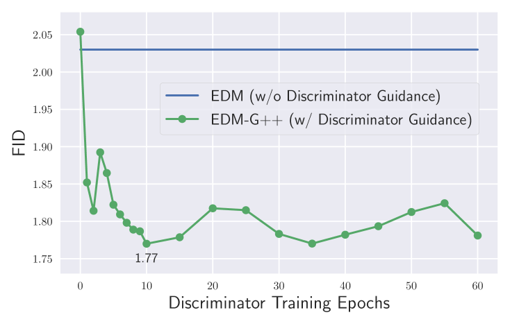
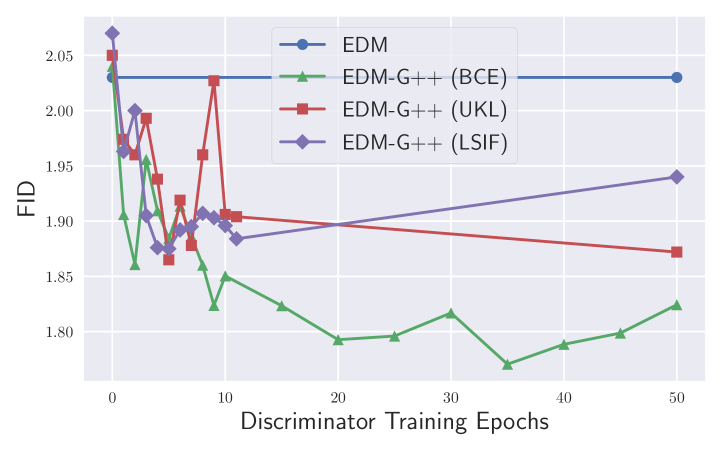
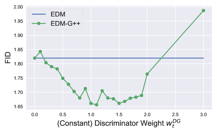
Figure 3: Discriminator guidance refines FID on CIFAR-10.

The correction term 𝐜𝜽(𝐱t,t)=logprt(𝐱t)p𝜽t(𝐱t)fragmentscfragmentsθ(x𝑡,t)fragmentsp𝑟𝑡(x𝑡)fragmentspfragmentsθ𝑡(x𝑡)\mathbf{c}_{\bm{\theta}_{\infty}}(\mathbf{x}_{t},t)=\nabla\log{\frac{p_{r}^{t}(\mathbf{x}_{t})}{p_{\bm{\theta}_{\infty}}^{t}(\mathbf{x}_{t})}} is intractable in general because the density-ratio prtp𝜽tfragmentsp𝑟𝑡fragmentspfragmentsθ𝑡\frac{p_{r}^{t}}{p_{\bm{\theta}_{\infty}}^{t}} is inaccessible. Therefore, we estimate this density-ratio by training a discriminator at all noise level t𝑡t. For discriminator training, we first draw fake samples from the generative process of Eq. (3) as many as data instances. Then we classify the real and fake data using the noise-embedded Binary Cross Entropy (BCE)

ϕ=λ(t)(𝔼prt(𝐱t)[logdϕ(𝐱t,t)]+𝔼p𝜽t(𝐱t)[log(1dϕ(𝐱t,t))])dt,fragmentsbold-italic-ϕ𝜆(𝑡)(𝔼fragmentsp𝑟𝑡(x𝑡)[𝑑bold-italic-ϕ(𝐱𝑡,𝑡)]𝔼fragmentspfragmentsθ𝑡(x𝑡)[(1𝑑bold-italic-ϕ(𝐱𝑡,𝑡))])d𝑡,\displaystyle\begin{split}\mathcal{L}_{\bm{\phi}}&=\int\lambda(t)\big{(}\mathbb{E}_{p_{r}^{t}(\mathbf{x}_{t})}[-\log{d_{\bm{\phi}}(\mathbf{x}_{t},t)}]\\ &\quad+\mathbb{E}_{p_{\bm{\theta}_{\infty}}^{t}(\mathbf{x}_{t})}[-\log{(1-d_{\bm{\phi}}(\mathbf{x}_{t},t))}]\big{)}\mathop{}\!\mathrm{d}t,\end{split} (4)

where λ𝜆\lambda is the temporal weight, see Algorithm 1 and Appendix A.4 for details.

As the correction term is represented by

𝐜𝜽(𝐱t,t)=logdϕ(𝐱t,t)1dϕ(𝐱t,t),fragmentscfragmentsθ(x𝑡,t)fragmentsdfragmentsϕ(x𝑡,t)fragments1dfragmentsϕ(x𝑡,t),\displaystyle\mathbf{c}_{\bm{\theta}_{\infty}}(\mathbf{x}_{t},t)=\nabla\log{\frac{d_{\bm{\phi}_{*}}(\mathbf{x}_{t},t)}{1-d_{\bm{\phi}_{*}}(\mathbf{x}_{t},t)}},

in terms of the optimal discriminator dϕfragmentsdfragmentsϕd_{\bm{\phi}_{*}} of ϕfragmentsLbold-italic-ϕ\mathcal{L}_{\bm{\phi}}, we estimate the correction term 𝐜𝜽fragmentscfragmentsθ\mathbf{c}_{\bm{\theta}_{\infty}} with a neural discriminator dϕfragmentsdbold-italic-ϕd_{\bm{\phi}} by

𝐜𝜽(𝐱t,t)𝐜ϕ(𝐱t,t):=logdϕ(𝐱t,t)1dϕ(𝐱t,t).fragmentscfragmentsθ(x𝑡,t)cbold-italic-ϕ(x𝑡,t)assignfragmentsdbold-italic-ϕ(x𝑡,t)fragments1dbold-italic-ϕ(x𝑡,t).\displaystyle\mathbf{c}_{\bm{\theta}_{\infty}}(\mathbf{x}_{t},t)\approx\mathbf{c}_{\bm{\phi}}(\mathbf{x}_{t},t):=\nabla\log{\frac{d_{\bm{\phi}}(\mathbf{x}_{t},t)}{1-d_{\bm{\phi}}(\mathbf{x}_{t},t)}}.

With the above tractable correction estimate, we define the Discriminator Guidance (DG) by

d𝐱tfragmentsdx𝑡\displaystyle\mathop{}\!\mathrm{d}\mathbf{x}_{t} =[𝐟(𝐱t,t)g2(t)(𝐬𝜽+𝐜ϕ)(𝐱t,t)]dt¯+g(t)d𝐰¯t.fragments[f(x𝑡,t)g2(t)(sfragmentsθcbold-italic-ϕ)(x𝑡,t)]d¯𝑡g(t)d¯𝐰𝑡.\displaystyle=\big{[}\mathbf{f}(\mathbf{x}_{t},t)-g^{2}(t)(\mathbf{s}_{\bm{\theta}_{\infty}}+\mathbf{c}_{\bm{\phi}})(\mathbf{x}_{t},t)\big{]}\mathop{}\!\mathrm{d}\bar{t}+g(t)\mathop{}\!\mathrm{d}\bar{\mathbf{w}}_{t}. (5)

Figure 3 shows that the discriminator indeed improves sample quality with a quick convergence.
Refer to caption
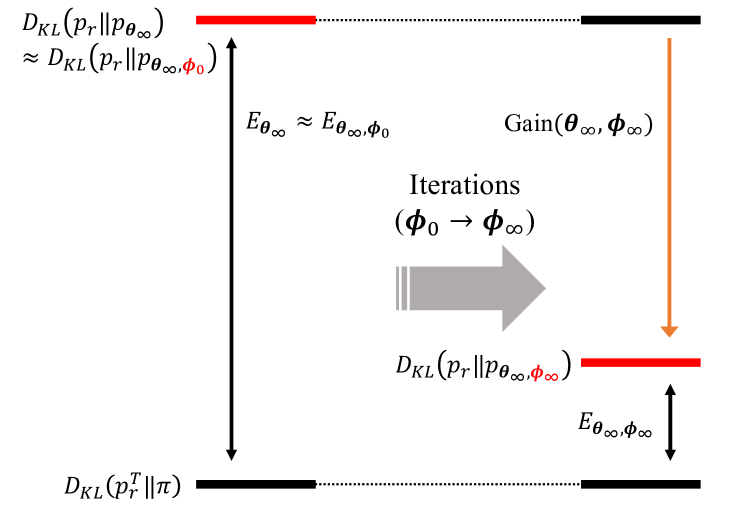
Figure 4: Schematic illustration of the analysis in Section 3.3. The gain increases as discriminator learns.

3.3 Theoretical Analysis

Although we introduced Discriminator Guidance in the context of differential equations, this section examines the approach from the perspective of statistical divergence between the data and the sample distributions. Specifically, we define p𝜽,ϕfragmentspfragmentsθ,ϕp_{\bm{\theta}_{\infty},\bm{\phi}} as the discriminator-guided sample distribution of Eq. (5). The central question becomes

Is p𝛉,ϕfragmentspfragmentsθ,ϕp_{\bm{\theta}_{\infty},\bm{\phi}} closer to the data distribution prfragmentsp𝑟p_{r} than p𝛉fragmentspfragmentsθp_{\bm{\theta}_{\infty}}?

We answer the question in Theorem 2.

Theorem 2.

If the assumptions of Theorem 1 hold, then

DKL(prp𝜽)=DKL(prTπ)+E𝜽,fragmentsDfragmentsKL(p𝑟pfragmentsθ)DfragmentsKL(p𝑟𝑇π)Efragmentsθ,\displaystyle D_{KL}(p_{r}\|p_{\bm{\theta}_{\infty}})=D_{KL}(p_{r}^{T}\|\pi)+E_{\bm{\theta}_{\infty}},
DKL(prp𝜽,ϕ)DKL(prTπ)+E𝜽,ϕ,fragmentsDfragmentsKL(p𝑟pfragmentsθ,ϕ)DfragmentsKL(p𝑟𝑇π)Efragmentsθ,ϕ,\displaystyle D_{KL}(p_{r}\|p_{\bm{\theta}_{\infty},\bm{\phi}})\leq D_{KL}(p_{r}^{T}\|\pi)+E_{\bm{\theta}_{\infty},\bm{\phi}},

where E𝛉fragmentsEfragmentsθE_{\bm{\theta}_{\infty}} is the score error

E𝜽=120Tg2(t)𝔼prt[logprt𝐬𝜽22]dt,fragmentsEfragmentsθ120𝑇g2(t)Efragmentsp𝑟𝑡[p𝑟𝑡sfragmentsθ22]dt,\displaystyle E_{\bm{\theta}_{\infty}}=\frac{1}{2}\int_{0}^{T}g^{2}(t)\mathbb{E}_{p_{r}^{t}}\big{[}\|\nabla\log{p_{r}^{t}}-\mathbf{s}_{\bm{\theta}_{\infty}}\|_{2}^{2}\big{]}\mathop{}\!\mathrm{d}t,

and E𝛉,ϕfragmentsEfragmentsθ,ϕE_{\bm{\theta}_{\infty},\bm{\phi}} is the discriminator-adjusted score error

E𝜽,ϕ=120Tg2(t)𝔼prt[logprt(𝐬𝜽+𝐜ϕ)22]dtfragmentsEfragmentsθ,ϕ120𝑇g2(t)Efragmentsp𝑟𝑡[p𝑟𝑡(sfragmentsθcbold-italic-ϕ)22]dt\displaystyle E_{\bm{\theta}_{\infty},\bm{\phi}}=\frac{1}{2}\int_{0}^{T}g^{2}(t)\mathbb{E}_{p_{r}^{t}}\big{[}\|\nabla\log{p_{r}^{t}}-(\mathbf{s}_{\bm{\theta}_{\infty}}+\mathbf{c}_{\bm{\phi}})\|_{2}^{2}\big{]}\mathop{}\!\mathrm{d}t
=120Tg2(t)𝔼prt[𝐜𝜽𝐜ϕ22]dt.fragments120𝑇g2(t)Efragmentsp𝑟𝑡[cfragmentsθcbold-italic-ϕ22]dt.\displaystyle\!\quad\quad\quad=\frac{1}{2}\int_{0}^{T}g^{2}(t)\mathbb{E}_{p_{r}^{t}}\big{[}\|\mathbf{c}_{\bm{\theta}_{\infty}}-\mathbf{c}_{\bm{\phi}}\|_{2}^{2}\big{]}\mathop{}\!\mathrm{d}t.
Table 1: Discriminator-adjusted score error E𝜽,ϕfragmentsEfragmentsθ,ϕE_{\bm{\theta}_{\infty},\bm{\phi}} and corresponding Gain.
Discriminator E𝜽,ϕfragmentsEfragmentsθ,ϕE_{\bm{\theta}_{\infty},\bm{\phi}} Gain
Blind dϕb(0.5)fragmentsdfragmentsϕ𝑏(0.5)d_{\bm{\phi}_{b}}(\equiv 0.5) E𝜽fragmentsEfragmentsθE_{\bm{\theta}_{\infty}} 0
Optimal dϕfragmentsdfragmentsϕd_{\bm{\phi}_{*}} 0 E𝜽fragmentsEfragmentsθE_{\bm{\theta}_{\infty}} (Maximum)
\cdashline1-3 Untrained dϕ0(0.5)fragmentsdfragmentsϕ0(0.5)d_{\bm{\phi}_{0}}(\approx 0.5) E𝜽fragmentsEfragmentsθ\approx E_{\bm{\theta}_{\infty}} 0fragments0\approx 0
Trained dϕfragmentsdfragmentsϕd_{\bm{\phi}_{\infty}} E𝜽fragmentsmuch-less-thanEfragmentsθ\ll E_{\bm{\theta}_{\infty}} E𝜽fragmentsEfragmentsθ\nearrow E_{\bm{\theta}_{\infty}}

To measure the effect of discriminator training, we use Theorem 2 to compute the gain by subtracting two KLs,


DKL(prp𝜽,ϕ)DKL(prp𝜽)Gain(𝜽,ϕ),fragmentsDfragmentsKL(p𝑟pfragmentsθ,ϕ)DfragmentsKL(p𝑟pfragmentsθ)Gain(θ,ϕ),\displaystyle D_{KL}(p_{r}\|p_{\bm{\theta}_{\infty},\bm{\phi}})\leq D_{KL}(p_{r}\|p_{\bm{\theta}_{\infty}})-\textup{Gain}(\bm{\theta}_{\infty},\bm{\phi}),

where Gain(𝜽,ϕ)=E𝜽E𝜽,ϕfragmentsGain(θ,ϕ)EfragmentsθEfragmentsθ,ϕ\textup{Gain}(\bm{\theta}_{\infty},\bm{\phi})=E_{\bm{\theta}_{\infty}}-E_{\bm{\theta}_{\infty},\bm{\phi}} represents the difference between the score error and the discriminator-adjusted score error. Note that while Theorem 2 does not guarantee that the gain is strictly positive, it is initialized near zero and gradually increases throughout discriminator training, as summarized in Table 3.3. Specifically, when the discriminator is completely blind (dϕb0.5fragmentsdfragmentsϕ𝑏0.5d_{\bm{\phi}_{b}}\equiv 0.5), there is no signal from the discriminator gradient, and the discriminator-adjusted score error E𝜽,ϕbfragmentsEfragmentsθ,ϕ𝑏E_{\bm{\theta}_{\infty},\bm{\phi}_{b}} equals the score error E𝜽fragmentsEfragmentsθE_{\bm{\theta}_{\infty}}. Therefore, the gain is approximately zero when the discriminator is untrained (dϕ00.5fragmentsdfragmentsϕ00.5d_{\bm{\phi}_{0}}\approx 0.5) as shown in Figure 3. On the other hand, at the optimal discriminator dϕfragmentsdfragmentsϕd_{\bm{\phi}_{*}}, the neural correction 𝐜ϕfragmentscfragmentsϕ\mathbf{c}_{\bm{\phi}_{*}} matches the target correction 𝐜𝜽fragmentscfragmentsθ\mathbf{c}_{\bm{\theta}_{\infty}} and satisfies E𝜽,ϕ=0fragmentsEfragmentsθ,ϕ0E_{\bm{\theta}_{\infty},\bm{\phi}_{*}}=0, allowing Gain to be maximized as discriminator parameters are updated. See Figure 4 for a schematic visualization.

In other words, we can interpret that Discriminator Guidance introduces an additional axial degree of freedom ϕbold-italic-ϕ\bm{\phi} that reparametrizes the score error E𝜽fragmentsEfragmentsθE_{\bm{\theta}_{\infty}} into a discriminator-adjusted score error E𝜽,ϕfragmentsEfragmentsθ,ϕE_{\bm{\theta}_{\infty},\bm{\phi}}. As a result, the score error E𝜽fragmentsEfragmentsθE_{\bm{\theta}_{\infty}} is no longer optimized with the denoising score loss 𝜽fragmentsL𝜽\mathcal{L}_{\bm{\theta}}, but the reparametrized error E𝜽,ϕfragmentsEfragmentsθ,ϕE_{\bm{\theta}_{\infty},\bm{\phi}} can be further optimized with an alternative loss ϕfragmentsLbold-italic-ϕ\mathcal{L}_{\bm{\phi}} of Eq. (4).

3.4 Optimality Analysis

Refer to caption
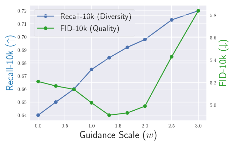
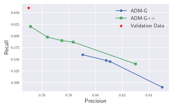
Figure 5: FID and Recall trade-off on DiT-XL-G++.

Let’s take a closer look at the score component. Our discriminator training is stable because we keep a pre-trained score model fixed during training, unlike unstable GAN training. Hence, after the discriminator has reached its optimal point, the resulting adjusted model score is given by

𝐬𝜽(𝐱t,t)+w𝐜ϕ(𝐱t,t)fragmentssfragmentsθ(x𝑡,t)wcfragmentsϕ(x𝑡,t)\displaystyle\mathbf{s}_{\bm{\theta}_{\infty}}(\mathbf{x}_{t},t)+w\mathbf{c}_{\bm{\phi}_{*}}(\mathbf{x}_{t},t)
=logp𝜽(𝐱t)+wlogprt(𝐱t)p𝜽t(𝐱t)fragmentspfragmentsθ(x𝑡)wfragmentsp𝑟𝑡(x𝑡)fragmentspfragmentsθ𝑡(x𝑡)\displaystyle\quad=\nabla\log{p_{\bm{\theta}_{\infty}}(\mathbf{x}_{t})}+w\nabla\log{\frac{p_{r}^{t}(\mathbf{x}_{t})}{p_{\bm{\theta}_{\infty}}^{t}(\mathbf{x}_{t})}}
=log[(prt(𝐱t))w(p𝜽t(𝐱t))1w],fragments[(p𝑟𝑡(x𝑡))𝑤(pfragmentsθ𝑡(x𝑡))fragments1w],\displaystyle\quad=\nabla\log{\big{[}(p_{r}^{t}(\mathbf{x}_{t}))^{w}(p_{\bm{\theta}_{\infty}}^{t}(\mathbf{x}_{t}))^{1-w}\big{]}},

Therefore, the sample distribution (prt)w(p𝜽t)1wfragments(p𝑟𝑡)𝑤(pfragmentsθ𝑡)fragments1w(p_{r}^{t})^{w}(p_{\bm{\theta}_{\infty}}^{t})^{1-w} balances data distribution and non-guided distribution. The argument also holds for the conditional case, leading DG as a controller for the intra-class diversity. Figure 5 experiments on ImageNet, demonstrating that there is a sweet spot of DG weight regarding both quality (FID) and diversity (recall).

3.5 Connection with Classifier Guidance

Classifier Guidance (CG) (Dhariwal & Nichol, 2021) is a milestone technique to guide a sample with a pre-trained classifier pψ(c|𝐱t,t)fragmentspfragmentsψ(c|x𝑡,t)p_{\psi_{\infty}}(c|\mathbf{x}_{t},t). The classifier-guided generative process is d𝐱t=[𝐟(𝐱t,t)g2(t)(𝐬𝜽(𝐱t,t)+logp𝝍(y|𝐱t,t))]dt¯+gtd𝐰¯tfragmentsdx𝑡[f(x𝑡,t)g2(t)(sfragmentsθ(x𝑡,t)pfragmentsψ(y|x𝑡,t))]d¯𝑡g𝑡d¯𝐰𝑡\mathop{}\!\mathrm{d}\mathbf{x}_{t}=[\mathbf{f}(\mathbf{x}_{t},t)-g^{2}(t)(\mathbf{s}_{\bm{\theta}_{\infty}}(\mathbf{x}_{t},t)+\nabla\log{p_{\bm{\psi}_{\infty}}(y|\mathbf{x}_{t},t)})]\mathop{}\!\mathrm{d}\bar{t}+g_{t}\mathop{}\!\mathrm{d}\bar{\mathbf{w}}_{t}. This is equivalent to sampling from the joint distribution of (𝐱t,y)fragments(x𝑡,y)(\mathbf{x}_{t},y) because

logprt(𝐱t,y)fragmentsp𝑟𝑡(x𝑡,y)\displaystyle\nabla\log{p_{r}^{t}(\mathbf{x}_{t},y)} =logprt(𝐱t)+logp(y|𝐱t,t)fragmentsp𝑟𝑡(x𝑡)p(y|x𝑡,t)\displaystyle=\nabla\log{p_{r}^{t}(\mathbf{x}_{t})}+\nabla\log{p(y|\mathbf{x}_{t},t)}
𝐬𝜽(𝐱t,t)+logp𝝍(y|𝐱t,t),fragmentssfragmentsθ(x𝑡,t)pfragmentsψ(y|x𝑡,t),\displaystyle\approx\mathbf{s}_{\bm{\theta}_{\infty}}(\mathbf{x}_{t},t)+\nabla\log{p_{\bm{\psi}_{\infty}}(y|\mathbf{x}_{t},t)},

where p(y|𝐱t,t)fragmentsp(y|x𝑡,t)p(y|\mathbf{x}_{t},t) is the oracle classifier at t𝑡t. Classifier Guidance provides supervision information on a sample path, evaluating whether the sample is correctly classified by the class label y𝑦y, or not. However, using Classifier Guidance may lead to mode collapse as it maximizes the classifier probability p(y|𝐱t,t)fragmentsp(y|x𝑡,t)p(y|\mathbf{x}_{t},t). In contrast, Discriminator Guidance offers enhanced mode coverage, as elaborated in Section 3.4, by providing distinctive supervision information on whether a sample path is realistic or not.

Algorithm 2 Sampling with Guidance Techniques
1: Sample 𝐱T𝒩(0,σmax2𝐈)fragmentsx𝑇similar-toN(0,σfragmentsmax2I)\mathbf{x}_{T}\sim\mathcal{N}(0,\sigma_{max}^{2}\mathbf{I})
2:for i=NfragmentsiNi=N to 111 do
3:    Sample ϵi𝒩(0,S12𝐈)fragmentsϵ𝑖similar-toN(0,S12I)\bm{\epsilon}_{i}\sim\mathcal{N}(0,S_{1}^{2}\mathbf{I}) and ϵi𝒩(0,𝐈)fragmentsϵ𝑖similar-toN(0,I)\bm{\epsilon}_{i}^{\prime}\sim\mathcal{N}(0,\mathbf{I})
4:    t^iσ1((1+γti)σ(ti))fragments^𝑡𝑖σfragments1((1γfragmentst𝑖)σ(t𝑖))\hat{t}_{i}\leftarrow\sigma^{-1}((1+\gamma_{t_{i}})\sigma(t_{i})) (Karras et al., 2022)
5:    𝐱t^i𝐱ti+σ2(t^i)σ2(ti)ϵtifragmentsxfragments^𝑡𝑖xfragmentst𝑖fragmentsσ2(^𝑡𝑖)σ2(t𝑖)ϵfragmentst𝑖\mathbf{x}_{\hat{t}_{i}}\leftarrow\mathbf{x}_{t_{i}}+\sqrt{\sigma^{2}(\hat{t}_{i})-\sigma^{2}(t_{i})}\bm{\epsilon}_{t_{i}}
6:    𝐬t^i𝐟(𝐱t^i,t^i)1+η22g2t^i𝐬𝜽(𝐱t^i,t^i)fragmentssfragments^𝑡𝑖f(xfragments^𝑡𝑖,^𝑡𝑖)fragments1η22g2fragments^𝑡𝑖sfragmentsθ(xfragments^𝑡𝑖,^𝑡𝑖)\mathbf{s}_{\hat{t}_{i}}\leftarrow\mathbf{f}(\mathbf{x}_{\hat{t}_{i}},\hat{t}_{i})-\frac{1+\eta^{2}}{2}g^{2}_{\hat{t}_{i}}\mathbf{s}_{\bm{\theta}_{\infty}}(\mathbf{x}_{\hat{t}_{i}},\hat{t}_{i})
7:    𝐜t^i1+η22g2t^ilogdϕ(ντt^i𝐱t^i,τt^i)1dϕ(ντt^i𝐱t^i,τt^i)fragmentscfragments^𝑡𝑖fragments1η22g2fragments^𝑡𝑖fragmentsdfragmentsϕ(νfragmentsτfragments^𝑡𝑖xfragments^𝑡𝑖,τfragments^𝑡𝑖)fragments1dfragmentsϕ(νfragmentsτfragments^𝑡𝑖xfragments^𝑡𝑖,τfragments^𝑡𝑖)\mathbf{c}_{\hat{t}_{i}}\leftarrow-\frac{1+\eta^{2}}{2}g^{2}_{\hat{t}_{i}}\nabla\log{\frac{d_{\bm{\phi}_{\infty}}(\nu_{\tau_{\hat{t}_{i}}}\mathbf{x}_{\hat{t}_{i}},\tau_{\hat{t}_{i}})}{1-d_{\bm{\phi}_{\infty}}(\nu_{\tau_{\hat{t}_{i}}}\mathbf{x}_{\hat{t}_{i}},\tau_{\hat{t}_{i}})}} (Eq. (8))
8:    𝐠t^i1+η22g2t^ilogp𝝍(y|𝐱t^i,t^i)fragmentsgfragments^𝑡𝑖fragments1η22g2fragments^𝑡𝑖pfragmentsψ(y|xfragments^𝑡𝑖,^𝑡𝑖)\mathbf{g}_{\hat{t}_{i}}\leftarrow-\frac{1+\eta^{2}}{2}g^{2}_{\hat{t}_{i}}\nabla\log{p_{\bm{\psi}_{\infty}}(y|\mathbf{x}_{\hat{t}_{i}},\hat{t}_{i})}
9:    𝐱ti1𝐱t^i+(ti1t^i)(𝐬t^i+wt^iDG𝐜t^i+wt^iCG𝐠t^i)fragmentsxfragmentstfragmentsi1xfragments^𝑡𝑖(tfragmentsi1^𝑡𝑖)(sfragments^𝑡𝑖wfragments^𝑡𝑖fragmentsDGcfragments^𝑡𝑖wfragments^𝑡𝑖fragmentsCGgfragments^𝑡𝑖)\mathbf{x}_{t_{i-1}}\leftarrow\mathbf{x}_{\hat{t}_{i}}+(t_{i-1}-\hat{t}_{i})\big{(}\mathbf{s}_{\hat{t}_{i}}+w_{\hat{t}_{i}}^{DG}\mathbf{c}_{\hat{t}_{i}}+w_{\hat{t}_{i}}^{CG}\mathbf{g}_{\hat{t}_{i}}\big{)}
10:    𝐱ti1𝐱ti1+ηgt^iti1t^iϵifragmentsxfragmentstfragmentsi1xfragmentstfragmentsi1ηgfragments^𝑡𝑖fragmentstfragmentsi1^𝑡𝑖ϵ𝑖\mathbf{x}_{t_{i-1}}\leftarrow\mathbf{x}_{t_{i-1}}+\eta g_{\hat{t}_{i}}\sqrt{t_{i-1}-\hat{t}_{i}}\bm{\epsilon}_{i}^{\prime}
11:end for

As sampling from the joint distribution of (𝐱t,y)fragments(x𝑡,y)(\mathbf{x}_{t},y) requires accurate score estimation, Discriminator Guidance and Classifier Guidance can be combined for a synergistic effect. We suggest the combination of guidance techniques by

d𝐱t=[𝐟(𝐱t,t)g2(t)((𝐬𝜽+wtDG𝐜ϕ)(𝐱t,t)+wtCGlogp𝝍(c|𝐱t,t))]dt¯+g(t)d𝐰¯t,fragmentsd𝐱𝑡[𝐟(𝐱𝑡,𝑡)𝑔2(𝑡)((𝐬fragmentsθ𝑤𝑡fragmentsDG𝐜fragmentsϕ)(𝐱𝑡,𝑡)𝑤𝑡fragmentsCG𝑝fragmentsψ(𝑐|𝐱𝑡,𝑡))]d¯𝑡𝑔(𝑡)d¯𝐰𝑡,\displaystyle\begin{split}\mathop{}\!\mathrm{d}\mathbf{x}_{t}&=\Big{[}\mathbf{f}(\mathbf{x}_{t},t)-g^{2}(t)\big{(}(\mathbf{s}_{\bm{\theta}_{\infty}}+w_{t}^{DG}\mathbf{c}_{\bm{\phi}_{\infty}})(\mathbf{x}_{t},t)\\ &\quad+w_{t}^{CG}\nabla\log{p_{\bm{\psi}_{\infty}}(c|\mathbf{x}_{t},t)}\big{)}\Big{]}\mathop{}\!\mathrm{d}\bar{t}+g(t)\mathop{}\!\mathrm{d}\bar{\mathbf{w}}_{t},\end{split} (6)
Table 2: Algorithm 2 includes DDPM, DDIM, and EDM samplers.
Sampler γtfragmentsγ𝑡\gamma_{t} η𝜂\eta wtCGfragmentsw𝑡fragmentsCGw_{t}^{CG} wtDGfragmentsw𝑡fragmentsDGw_{t}^{DG}
DDPM 0 1 0 0
DDIM 0 0 0 0
EDM \geq0 0 0 0
ADM-G 0 1 >>0 0
\cdashline1-5 EDM-G++ \geq0 0 0 >>0
ADM-G++ 0 1 >>0 >>0

where wtDGfragmentsw𝑡fragmentsDGw_{t}^{DG} and wtCGfragmentsw𝑡fragmentsCGw_{t}^{CG} are the time-dependent weights, respectively. The two pieces of information could ideally guide the sample toward the common likely region of classifier and discriminator in a complementary way.

Algorithm 2 describes the full details of our sampling procedure for Eq. (6). The algorithm reduces the samplers of DDPM (Ho et al., 2020; Dhariwal & Nichol, 2021), DDIM (Song et al., 2020a), and EDM (Karras et al., 2022) with corresponding hyperparameters in Table 3.5. Our sampler is denoted as the postfix with G++ upon a basic sampler by a prefix. See Appendix D.1 for detailed sampling procedure.

4 Related Works

A line of research merges diffusion models with GAN models. Zheng et al. (2022b); Lyu et al. (2022) synthesize the diffused data 𝐱σmidfragmentsxfragmentsσfragmentsmid\mathbf{x}_{\sigma_{mid}} with a GAN generator (by putting 𝐱Tfragmentsx𝑇\mathbf{x}_{T} as generator’s input), and denoise 𝐱σmidfragmentsxfragmentsσfragmentsmid\mathbf{x}_{\sigma_{mid}} to 𝐱0fragmentsx0\mathbf{x}_{0} with a diffusion model. Xiao et al. (2022) exchange thousands of denoising steps with a small number of sequential conditional GAN generators. Wang et al. (2022) utilize the diffusion concept to train GAN. On the contrary, Jolicoeur-Martineau et al. (2021) train the diffusion model with an adversarial loss. The diffusion model and GAN in previous works, however, do not interplay with each other in generation process after their training. In contrast, the discriminator in DG intervenes in generation process, directly. Another difference to previous research is that we train our discriminator without any generator, so discriminator training is stable.
Refer to caption
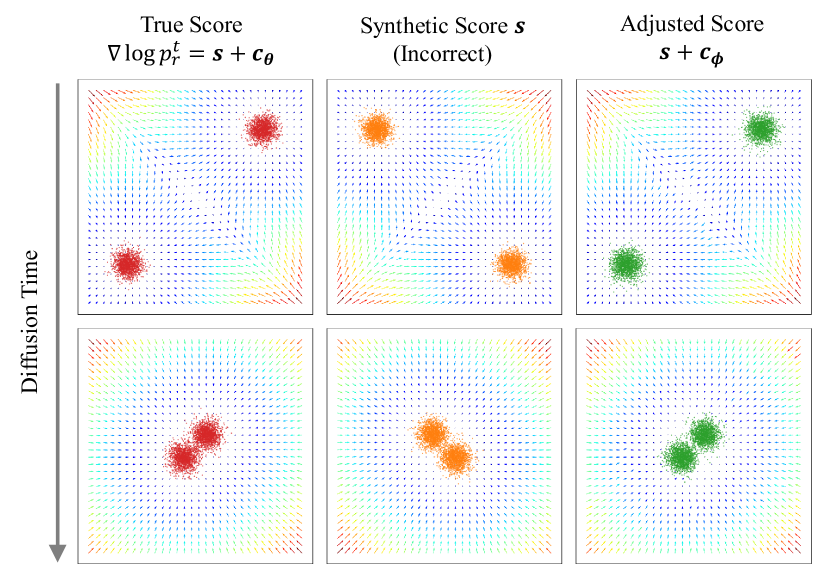
Figure 6: Comparison of the true data score, synthetic score, and adjusted score in a toy 2-dimensional case. We assume pr(𝐱):=12𝒩(𝐱;(10,10)T,𝐈)+12𝒩(𝐱;(10,10)T,𝐈)fragmentsp𝑟(x)assign12N(x;(10,10)𝑇,I)12N(x;(10,10)𝑇,I)p_{r}(\mathbf{x}):=\frac{1}{2}\mathcal{N}(\mathbf{x};(10,10)^{T},\mathbf{I})+\frac{1}{2}\mathcal{N}(\mathbf{x};(-10,-10)^{T},\mathbf{I}) as data distribution and pg(𝐱):=12𝒩(𝐱;(10,10)T,𝐈)+12𝒩(𝐱;(10,10)T,𝐈)fragmentsp𝑔(x)assign12N(x;(10,10)𝑇,I)12N(x;(10,10)𝑇,I)p_{g}(\mathbf{x}):=\frac{1}{2}\mathcal{N}(\mathbf{x};(10,-10)^{T},\mathbf{I})+\frac{1}{2}\mathcal{N}(\mathbf{x};(-10,10)^{T},\mathbf{I}) as hypothetially synthesized generative distribution with an incorrect score 𝐬(𝐱t,t):=logpgt(𝐱t)fragmentss(x𝑡,t)assignp𝑔𝑡(x𝑡)\mathbf{s}(\mathbf{x}_{t},t):=\nabla\log{p_{g}^{t}(\mathbf{x}_{t})}. We solve the probability-flow ODE (Song et al., 2020b) to visualize samples from each score function.

Other previous works use the rejection sampler or MCMC to draw samples from a reweighted model distribution. Azadi et al. (2019); Che et al. (2020) utilize the rejection sampler to adjust the generator implicit distribution with the discriminator under the likelihood-ratio trick (Gutmann & Hyvärinen, 2010). Similarly, Turner et al. (2019) make use of likelihood-ratio trick to sample with MCMC. Specifically, Aneja et al. (2021) and Bauer & Mnih (2019) introduce the importance and rejection samplings from the aggregate posterior in VAE, respectively. In diffusion context, Discriminator Guidance maximizes prtp𝜽tfragmentsp𝑟𝑡fragmentspfragmentsθ𝑡\frac{p_{r}^{t}}{p_{\bm{\theta}_{\infty}}^{t}} in the same spirit of gradient ascent, and it could be interpreted as reweighting the model distribution p𝜽tfragmentspfragmentsθ𝑡p_{\bm{\theta}_{\infty}}^{t} with an importance weight of prtp𝜽tfragmentsp𝑟𝑡fragmentspfragmentsθ𝑡\frac{p_{r}^{t}}{p_{\bm{\theta}_{\infty}}^{t}}. Consequently, DG does not require sample rejection and is becoming scalable to high-dimensions.

5 Experiments

5.1 A Toy 2-dimensional Case

Table 3: Performance on CIFAR-10.
Model Diffusion Space NFE\downarrow Unconditional Conditional
NLL\downarrow FID\downarrow FID\downarrow
VDM (Kingma et al., 2021) Data 1000 2.49 7.41 -
DDPM (Ho et al., 2020) Data 1000 3.75 3.17 -
iDDPM (Nichol & Dhariwal, 2021) Data 1000 3.37 2.90 -
Soft Truncation (Kim et al., 2022b) Data 2000 2.91 2.47 -
INDM (Kim et al., 2022a) Latent 2000 3.09 2.28 -
CLD-SGM (Dockhorn et al., 2022) Data 312 3.31 2.25 -
NCSN++ (Song et al., 2020b) Data 2000 3.45 2.20 -
LSGM (Vahdat et al., 2021) Latent 138 3.43 2.10 -
NCSN++-G (Chao et al., 2022) Data 2000 - - 2.25
EDM (random seed) Data 39 2.60 2.03 1.82
EDM (reported, manual seed) Data 35 2.60 1.97 1.79
\cdashline1-6 LSGM-G++ Latent 138 3.42 1.94 -
EDM-G++ Data 35 2.55 1.77 1.64
  • We recalculate FID of EDM (Karras et al., 2022) under a random seed for a fair comparison with previous research. We report our performances under the random seed by default.

Table 4: Performance on CelebA/FFHQ 64x64.
Model NFE\downarrow CelebA FFHQ
DDPM++ (Song et al., 2020b) 131 2.32 -
Soft Truncation (Kim et al., 2022b) 131 1.90 -
Soft Diffusion (Daras et al., 2022) 300 1.85 -
INDM (Kim et al., 2022a) 132 1.75 -
Diffusion StyleGAN2 (Wang et al., 2022) 1 1.69 -
EDM (Karras et al., 2022) 79 - 2.39
\cdashline1-4 Soft Truncation-G++ 131 1.34 -
EDM-G++ 71 - 1.98

Figure 6 shows the experimental result of a tractable 2-dimensional toy case. We train a 4-layered MLP discriminator with 256 neurons until convergence, and we hypothesize an incorrect score function 𝐬:=logpgtfragmentssassignp𝑔𝑡\mathbf{s}:=\nabla\log{p_{g}^{t}} (for a synthetic generative distribution pgfragmentsp𝑔p_{g}) that misfits to the data score. If there is no guidance, the incorrect score 𝐬𝐬\mathbf{s} will generate samples from a wrong distribution as in Figure 6. On the contrary, 𝐬+𝐜ϕfragmentsscfragmentsϕ\mathbf{s}+\mathbf{c}_{\bm{\phi}_{\infty}} successfully guides 𝐬𝐬\mathbf{s} to logprtfragmentsp𝑟𝑡\nabla\log{p_{r}^{t}}, see Figures 15 and 16 for additional visualization.

5.2 Image Generation

We experiment on CIFAR-10, CelebA/FFHQ 64x64, and ImageNet 256x256. We use the pre-trained networks on CIFAR-10 and FFHQ from Karras et al. (2022); Vahdat et al. (2021), CelebA from Kim et al. (2022b) and ImageNet from Dhariwal & Nichol (2021); Peebles & Xie (2022).

Discriminator Network. We use the encoder of U-Net structure111We tested MLP, ResNet18, and a transformer, but the U-Net performed the best for Discriminator Guidance. as our discriminator network. For diffusion models on data space, we attach two noise-embedded U-Net encoders: the pre-trained ADM classifier (Dhariwal & Nichol, 2021) and an auxiliary (shallow) U-Net encoder. We put (𝐱t,t)fragments(x𝑡,t)(\mathbf{x}_{t},t) to the ADM classifier, and we extract the latent 𝐳tfragmentsz𝑡\mathbf{z}_{t} of 𝐱tfragmentsx𝑡\mathbf{x}_{t} from the last pooling layer of the pre-trained classifier. Then, we put (𝐳t,t)fragments(z𝑡,t)(\mathbf{z}_{t},t) to the auxiliary U-Net encoder and predict real/fake by its output. We freeze the ADM classifier, and we only fine-tune shallow U-Net encoder as default. Not to mention that fine-tuning save the training cost, fine-tuning performs better or equivalent to training the entire architecture (Kato & Teshima, 2021). For LSGM-G++, we train the U-Net encoder from scratch. For DiT-XL-G++, we train the latent classifier with the same architecture of the ADM classifier except the input dimension, and fine-tuning the shallow U-Net encoder for discriminator. We train a class-conditional discriminator for the class-conditional generation. See Table 8 for detailed training configuration.

Table 5: Performance on ImageNet 256x256.
Model Diffusion Space FID\downarrow sFID\downarrow IS\uparrow Prec\uparrow Rec\uparrow F1\uparrow
Validation Data 1.68 3.67 232.21 0.75 0.66 0.70
ADM (Dhariwal & Nichol, 2021) Data 10.94 6.02 100.98 0.69 0.63 0.66
DiT-XL/2 (Peebles & Xie, 2022) Latent 9.62 6.85 121.50 0.67 0.67 0.67
ADM-G (Dhariwal & Nichol, 2021) Data 4.59 5.25 186.70 0.82 0.52 0.64
RIN (Jabri et al., 2022) Data 4.51 - 161.00 - - -
LDM-4-G (Rombach et al., 2022) Latent 3.60 - 247.67 0.87 0.48 0.62
RIN + schedule (Chen, 2023) Data 3.52 - 186.20 - - -
simple diffusion (Hoogeboom et al., 2023) Data 2.77 - 211.80 - - -
DiT-XL/2-G (Peebles & Xie, 2022) Latent 2.27 4.60 278.24 0.83 0.57 0.68
\cdashline1-8 ADM-G++ Data 3.18 4.53 255.74 0.84 0.53 0.66
DiT-XL/2-G++ Latent 1.83 5.16 281.53 0.78 0.64 0.70
Table 6: Component-wise computational budget.
Dataset (Model) Score Training Sample Generation Discriminator Training
CIFAR-10 (EDM) 200M 𝐬𝜽fragmentssfragmentsθ\mathbf{s}_{\bm{\theta}_{\infty}} (480hr) 1.75M 𝐬𝜽fragmentssfragmentsθ\mathbf{s}_{\bm{\theta}_{\infty}} (1hr) 1M dϕfragmentsdbold-italic-ϕd_{\bm{\phi}} (10min)
ImageNet 256x256 (ADM) 2.5T 𝐬𝜽fragmentssfragmentsθ\mathbf{s}_{\bm{\theta}_{\infty}} 100M 𝐬𝜽fragmentssfragmentsθ\mathbf{s}_{\bm{\theta}_{\infty}} 25.6M dϕfragmentsdbold-italic-ϕd_{\bm{\phi}}
Refer to caption
(a) Original Data
Refer to caption
(b) EDM
Refer to caption
(c) EDM-G++
Figure 7: Comparison of (a) original sample, and the average of 100 regenerated samples of (b) EDM and (c) EDM-G++ on FFHQ. The regeneration FID is 1.25 (w/o DG) and 1.09 (w/ DG) if we perturb data by the standard Gaussian.

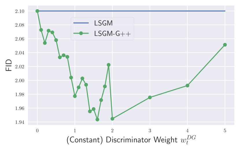
Quantitative Analysis. We achieve new SOTA FIDs on all datasets including CIFAR-10, CelebA, FFHQ, and ImageNet. On CIFAR-10, Table 5.1 shows that Discriminator Guidance is effective in both data diffusion (EDM) and latent diffusion (LSGM) models. Other than Discriminator Guidance, we use all the hyperparameters of EDM and LSGM, so the performance gain purely comes from the discriminator componenet. The gain of Discriminator Guidance is also notable on human-face datasets in Table 5.1.

On ImageNet 256x256, we present SOTA results in various metrics, including FID, sFID, IS, and recall in Table 5.2. For reference, we also measure these metrics on the ImageNet 50k validation data. Notably, IS and precision of the validation data are on par with the best models. Thus, optimizing other metrics, such as FID, sFID, and recall, becomes more important once IS and precision of a model reach the level of the validation data. Our experiments show that with Discriminator Guidance, we achieve the strongest performances with respect to FID and recall in DiT-XL/2-G++, indicating that the sample quality and diversity are significantly improved. See Table 8 for detailed hyperparameters and Appendix D.4 for uncurated samples.

In terms of carbon footprint, Discriminator Guidance requires additional sampling from the pre-trained score model plus discriminator training. Table 6 summarizes the component-wise neural network evaluation budget. In both CIFAR-10 and ImageNet experiments, Discriminator Guidance requires a lightweight burden compared to score training. Furthermore, we measure the actual elapsed time in GPU (A100) hours, including backpropagation time.

Qualitative Analysis. Figure 7 illustrates a comparison between the original sample and the averages of its regenerated samples (Meng et al., 2021) on FFHQ. If the score estimation is correct, the average reconstructed image should be approximately equal to the original image when the perturbation noise is small enough. To explain this, suppose the original image is 𝐲𝐲\mathbf{y} and we perturb it with a fixed direction ϵbold-italic-ϵ\bm{\epsilon} by 𝐲+σ(t)ϵfragmentsyσ(t)ϵ\mathbf{y}+\sigma(t)\bm{\epsilon}. Then, by putting this perturbed data into the Tweedie’s formula (Robbins, 1992; Jolicoeur-Martineau et al., 2021), the average reconstructed data 𝐱0fragmentsx0\mathbf{x}_{0} becomes

𝔼[𝐱0|𝐱t=𝐲+σ(t)ϵ]fragmentsE[x0|x𝑡yσ(t)ϵ]\displaystyle\mathbb{E}[\mathbf{x}_{0}|\mathbf{x}_{t}=\mathbf{y}+\sigma(t)\bm{\epsilon}]
=𝐲+σ(t)ϵ+σ2(t)logprt(𝐲+σ(t)ϵ).fragmentsyσ(t)ϵσ2(t)p𝑟𝑡(yσ(t)ϵ).\displaystyle\quad\quad\quad=\mathbf{y}+\sigma(t)\bm{\epsilon}+\sigma^{2}(t)\nabla\log{p_{r}^{t}\big{(}\mathbf{y}+\sigma(t)\bm{\epsilon}\big{)}}.

If σ(t)fragmentsσ(t)\sigma(t) is sufficiently small, we obtain prt(𝐲+σ(t)ϵ)p(ϵ)fragmentsp𝑟𝑡(yσ(t)ϵ)proportional-tosimilar-top(ϵ)p_{r}^{t}(\mathbf{y}+\sigma(t)\bm{\epsilon})\mathrel{\vbox{ \offinterlineskip\halign{\hfil$#$\cr\propto\cr\kern 2.0pt\cr\sim\cr\kern-2.0pt\cr}}}p(\bm{\epsilon}), which leads to 𝔼ϵ[logprt(𝐲+σ(t)ϵ)]0fragmentsEbold-italic-ϵ[p𝑟𝑡(yσ(t)ϵ)]0\mathbb{E}_{\bm{\epsilon}}[\nabla\log{p_{r}^{t}(\mathbf{y}+\sigma(t)\bm{\epsilon})}]\approx 0. Therefore, the average reconstructed image of 𝐲𝐲\mathbf{y} with a random direction ϵbold-italic-ϵ\bm{\epsilon} would approximately be the original data,

𝔼ϵ[𝔼[𝐱0|𝐱t=𝐲+σ(t)ϵ]]𝐲.fragmentsEbold-italic-ϵ[E[x0|x𝑡yσ(t)ϵ]]y.\displaystyle\mathbb{E}_{\bm{\epsilon}}\big{[}\mathbb{E}[\mathbf{x}_{0}|\mathbf{x}_{t}=\mathbf{y}+\sigma(t)\bm{\epsilon}]\big{]}\approx\mathbf{y}.

In conclusion, the closeness of the average reconstructed image to the original one indirectly diagnose whether the estimated score is accurate because the above argument holds for data score. Figure 7, with a small σ(t)=1fragmentsσ(t)1\sigma(t)=1, suggests that the adjusted score provides a more accurate estimation compared to the original model score.
Refer to caption
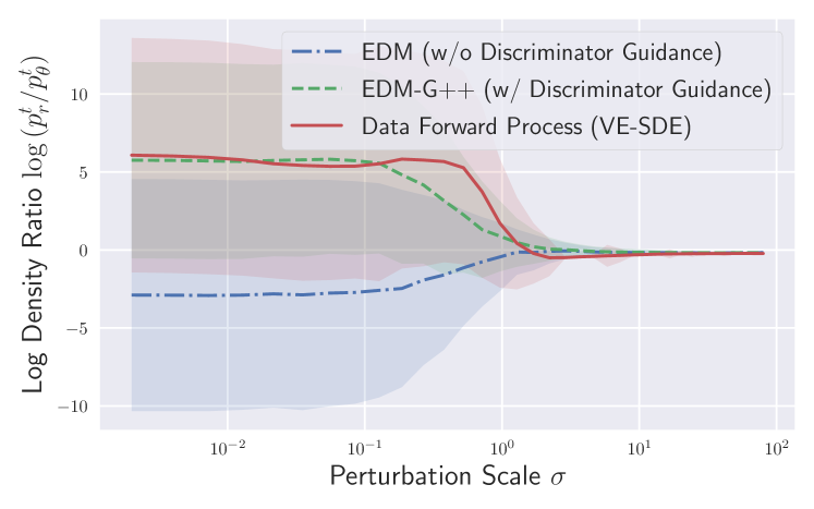
Figure 8: Comparison of sample trajectories with respect to the density-ratio on FFHQ.
Refer to caption
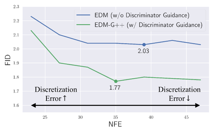
Figure 9: Ablation study for NFE on CIFAR-10.
Refer to caption
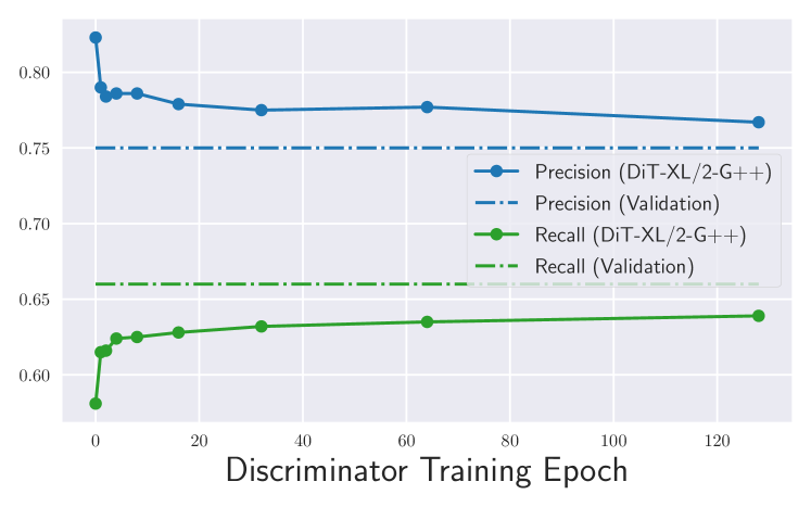
Figure 10: Precision/recall by discriminator training.
Refer to caption
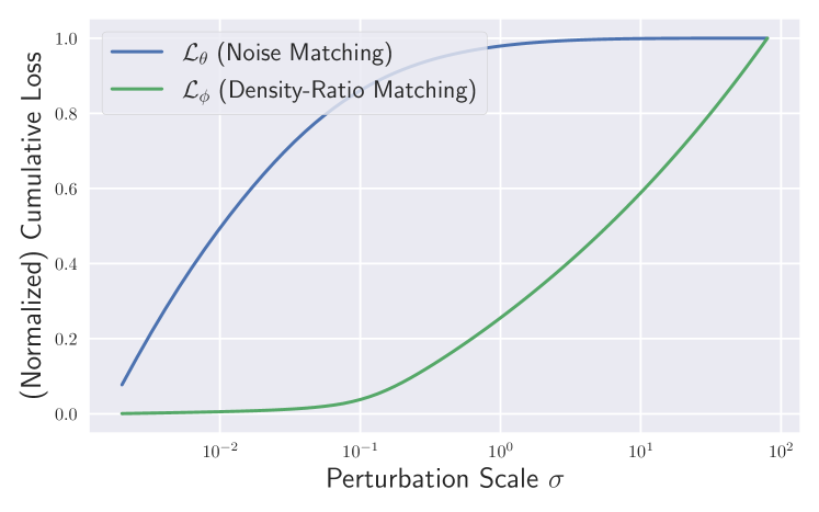
Figure 11: Loss contribution by noise scale.

Figure 8 shows that the trained discriminator is able to accurately distinguish between the diffusion path of real data and the denoising path of the generated sample. In contrast, the discriminator-adjusted denoising path deceives the discriminator, resulting in the density-ratio curve of the adjusted generative SDE (Eq. 5) closely approximating that of the data forward SDE.

Figure 9 illustrates the effect of Discriminator Guidance with respect to the sampling NFEs on CIFAR-10. As NFE decreases, the discretization error dominates the sampling error (De Bortoli, 2022), and the gain from Discriminator Guidance becomes suboptimal. We leave it as a future work to fit Discriminator Guidance on samplers with extremely small NFEs. See Appendix D.3 for more ablation studies.

Figure 10 shows the precision and recall curve by discriminator training. At the zero-th epoch, before discriminator training, we observe that precision/recall for vanilla DiT-XL-G are higher/lower than those of the validation data, respectively. This is because Classifier Guidance generates overconfident samples in terms of the classifier. However, Discriminator Guidance significantly mitigates this precision-recall trade-off of Classifier Guidance.

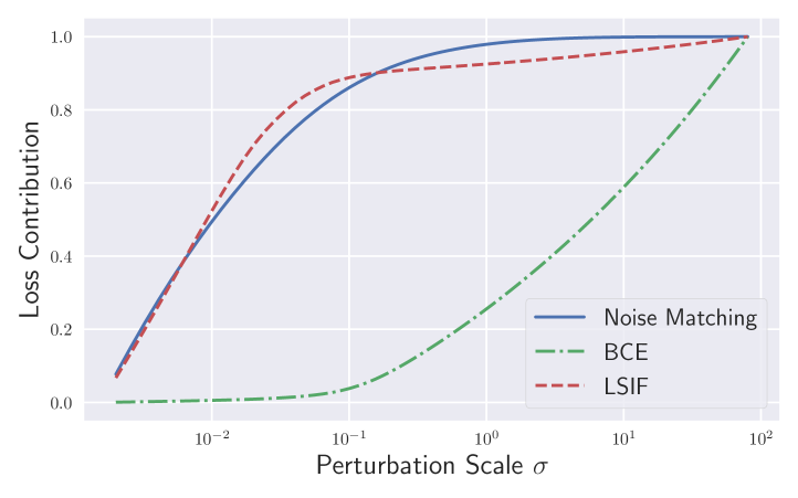
Figure 11 displays the normalized cumulative objective loss by noise scale. To ensure a fair comparison, we utilize the same weighting function ξ(t)=λ(t)fragmentsξ(t)λ(t)\xi(t)=\lambda(t) to evaluate the discriminator loss ϕfragmentsLbold-italic-ϕ\mathcal{L}_{\bm{\phi}} and the score loss 𝜽fragmentsL𝜽\mathcal{L}_{\bm{\theta}}. The results reveal that the discriminator can capture the estimation error, particularly at a large diffusion time that determines the sample diversity. This finding highlights the potential of Discriminator Guidance as a supplementary approach to address the problem of poor estimation at large time (Kim et al., 2022b) in the score matching framework.
Refer to caption
(a) SDEdit+DG improves translation quality
Refer to caption
(b) Realism vs. Faithfulness
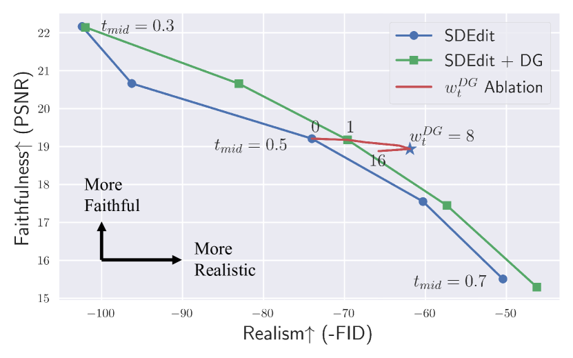
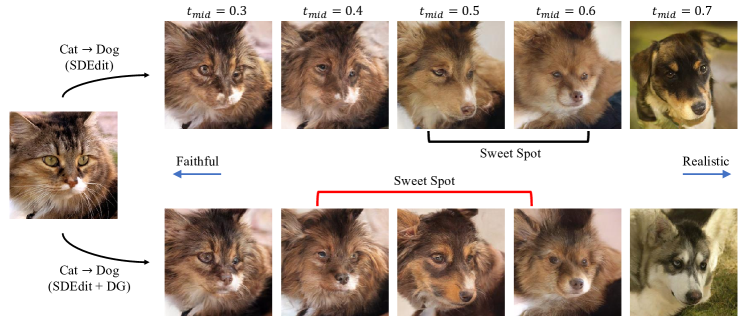
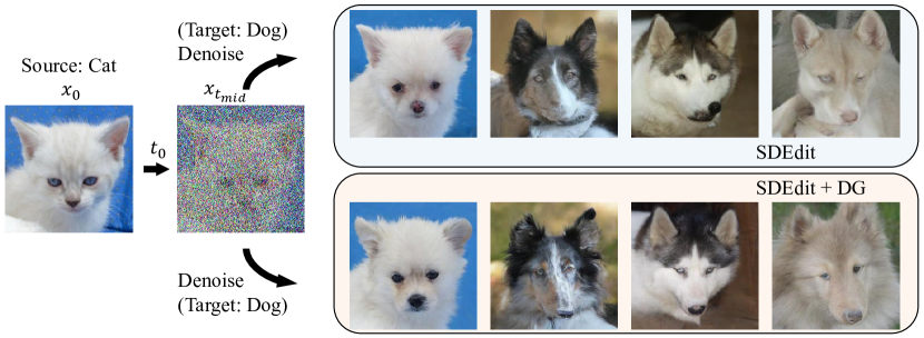
Figure 12: I2I translation task. (a) The discriminator-guided translated samples from SDEdit are more realistic than non-guided samples from SDEdit given the same translation starting time tmid=0.5fragmentstfragmentsmid0.5t_{mid}=0.5. (b) DG partially mitigates the trade-off between realism and faithfulness. Also, the weighted DG improves sample realism without hurting faithfulness.

5.3 Image-2-Image Translation

Discriminator Guidance could be applied to the Image-2-Image (I2I) translation task. I2I (Meng et al., 2021) denoise a perturbed source image with a score network trained on the target domain. For discriminator training, we first translate source training images, and then we aggregate these translated images with source images to a fake dataset 𝒢𝒢\mathcal{G}. By specifying 𝒟𝒟\mathcal{D} as target images, we follow Algorithm 1 to train the discriminator. Discriminator Guidance avoids going neither the source domain nor the translated domain, and it leads to the target domain. Empirically, the curve in Figure 12-(b) shows that our approach remedies the trade-off between realism (to target) and faithfulness (with source). We leave Appendix C for details.

6 Discussion

Table 7: Ablation study for hh-function on CIFAR-10.
Model Density-Ratio Matching Dh(r𝜽rϕ)fragmentsD(rfragmentsθrbold-italic-ϕ)D_{h}(r_{\bm{\theta}_{\infty}}\|r_{\bm{\phi}}) FID
EDM - 2.03
\cdashline1-3 EDM-G++ UKL (Nguyen et al., 2010) h(r)=rlogrrfragmentsh(r)rrrh(r)=r\log{r}-r 1.84
\cdashline2-3 LSIF (Kanamori et al., 2009) h(r)=(r1)2/2fragmentsh(r)(r1)22h(r)=(r-1)^{2}/2 1.84
\cdashline2-3 BCE (ϕfragmentsLbold-italic-ϕ\mathcal{L}_{\bm{\phi}} of Eq. 4) h(r)=rlogr(r+1)log(1+r)fragmentsh(r)rr(r1)(1r)h(r)=r\log{r}-(r+1)\log{(1+r)} 1.77

This section discusses two possible avenues for the future development of Discriminator Guidance. The first direction involves rewriting our approach in terms of Bregman divergence, while the second direction explores the simultaneous training of score and discriminator networks. In the first direction, the density-ratio r𝜽t=prtp𝜽tfragmentsrfragmentsθ𝑡fragmentsp𝑟𝑡fragmentspfragmentsθ𝑡r_{\bm{\theta}_{\infty}}^{t}=\frac{p_{r}^{t}}{p_{\bm{\theta}_{\infty}}^{t}} is the target of the discriminator, and BCE loss ϕfragmentsLbold-italic-ϕ\mathcal{L}_{\bm{\phi}} can be generalized into the family of hh-Bregman divergence (Sugiyama et al., 2012)

Dh(r𝜽rϕ)fragmentsD(rfragmentsθrbold-italic-ϕ)\displaystyle D_{h}(r_{\bm{\theta}_{\infty}}\|r_{\bm{\phi}}) =λ(t)𝔼p𝜽t(𝐱t)[h(r𝜽t(𝐱t))h(rϕt(𝐱t))fragmentsλ(t)Efragmentspfragmentsθ𝑡(x𝑡)[h(rfragmentsθ𝑡(x𝑡))h(rbold-italic-ϕ𝑡(x𝑡))\displaystyle=\int\lambda(t)\mathbb{E}_{p_{\bm{\theta}_{\infty}}^{t}(\mathbf{x}_{t})}\big{[}h(r_{\bm{\theta}_{\infty}}^{t}(\mathbf{x}_{t}))-h(r_{\bm{\phi}}^{t}(\mathbf{x}_{t}))
h(rϕt(𝐱t))(r𝜽t(𝐱t)rϕt(𝐱t))]dt,fragmentsh(rbold-italic-ϕ𝑡(x𝑡))(rfragmentsθ𝑡(x𝑡)rbold-italic-ϕ𝑡(x𝑡))]dt,\displaystyle\quad-\partial h(r_{\bm{\phi}}^{t}(\mathbf{x}_{t}))(r_{\bm{\theta}_{\infty}}^{t}(\mathbf{x}_{t})-r_{\bm{\phi}}^{t}(\mathbf{x}_{t}))\big{]}\mathop{}\!\mathrm{d}t,

where rϕ=dϕ1dϕfragmentsrbold-italic-ϕfragmentsdbold-italic-ϕfragments1dbold-italic-ϕr_{\bm{\phi}}=\frac{d_{\bm{\phi}}}{1-d_{\bm{\phi}}}. It is worth noting that the BCE loss is the unique divergence that belongs to both the hh-Bregman divergence and the f𝑓f-divergence (Amari, 2009). Therefore, our approach suggests a new divergence family for score estimation, see Appendix B for more discussion. Table 6 presents an experiment on Bregmena divergence.
Refer to caption
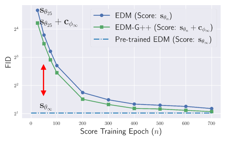
Figure 13: FID of simultaneous training on CIFAR-10.

Another potential direction is the simultaneous training of discriminator and score networks, which could be more appealing than GAN as it is a min-min problem instead of a mini-max GAN problem. However, the loss functions of 𝜽fragmentsL𝜽\mathcal{L}_{\bm{\theta}} and ϕfragmentsLbold-italic-ϕ\mathcal{L}_{\bm{\phi}} are independent, so their joint interplay would be restricted. The discriminator only marginally enhances the score accuracy, as shown in Figure 13.

As an alternative, we could modify the score loss to an f𝑓f-divergence (Song et al., 2021)

Df(pr(𝐱0)p𝜽(𝐱0))=Df(prT(𝐱T)π(𝐱T))+E𝜽,ϕf,fragmentsD𝑓(p𝑟(x0)p𝜽(x0))D𝑓(p𝑟𝑇(x𝑇)π(x𝑇))Efragmentsθ,ϕ𝑓,\displaystyle D_{f}(p_{r}(\mathbf{x}_{0})\|p_{\bm{\theta}}(\mathbf{x}_{0}))=D_{f}(p_{r}^{T}(\mathbf{x}_{T})\|\pi(\mathbf{x}_{T}))+E_{\bm{\theta},\bm{\phi}}^{f},

where E𝜽,ϕf=120Tg2(t)𝔼[f(prt(𝐱t)p𝜽t(𝐱t))prt(𝐱t)p𝜽t(𝐱t)logprt(𝐱t)𝐬𝜽(𝐱t,t)22]dtfragmentsEfragmentsθ,ϕ𝑓120𝑇g2(t)E[ffragments(fragmentsp𝑟𝑡(x𝑡)fragmentsp𝜽𝑡(x𝑡))fragmentsp𝑟𝑡(x𝑡)fragmentsp𝜽𝑡(x𝑡)p𝑟𝑡(x𝑡)s𝜽(x𝑡,t)22]dtE_{\bm{\theta},\bm{\phi}}^{f}=\frac{1}{2}\int_{0}^{T}g^{2}(t)\mathbb{E}\big{[}f^{\prime\prime}\big{(}\frac{p_{r}^{t}(\mathbf{x}_{t})}{p_{\bm{\theta}}^{t}(\mathbf{x}_{t})}\big{)}\frac{p_{r}^{t}(\mathbf{x}_{t})}{p_{\bm{\theta}}^{t}(\mathbf{x}_{t})}\|\nabla\log{p_{r}^{t}(\mathbf{x}_{t})}-\mathbf{s}_{\bm{\theta}}(\mathbf{x}_{t},t)\|_{2}^{2}\big{]}\mathop{}\!\mathrm{d}t given assumptions of Theorem 1. This f𝑓f-divergence estabilishes a connection between discriminator and score losses when using a neural ratio to approximate the true likelihood-ratio. The f𝑓f-divergence allows better score estimation in perceptually plausible region by weighting the score matching more on the spatial domain with high density-ratio prtp𝜽tfragmentsp𝑟𝑡fragmentsp𝜽𝑡\frac{p_{r}^{t}}{p_{\bm{\theta}}^{t}}, which could be an advantage over KL divergence training. We leave it as future work.

7 Conclusion

This paper refines the denoising process with an adjusted score estimation. With the proposed method, we could further optimize the divergence of a pre-trained score model. Empirical results demonstrate that our approach achieves new SOTA FIDs on all datasets. The deepfake images are one of the potential risks of the negative usage of this work.

Acknowledgements

This work was supported by Institute of Information &\& communications Technology Planning &\& Evaluation (IITP) grant funded by the Korea government(MSIT) (NO. 2022-0-00077, AI Technology Development for Commonsense Extraction, Reasoning, and Inference from Heterogeneous Data). Also, this work was supported by the National Research Foundation of Korea (NRF) grant funded by the Korea government(MSIT) (NRF-2019R1A5A1028324). We thank to Jiaming Song for his sincere advice to our work. We also thank to Byunghu Na and Seungjae Shin for their warm and keen feedbacks on our manuscript.

References

  • Amari (2009) Amari, S.-I. alphafragmentsalphaalpha-divergence is unique, belonging to both f𝑓f-divergence and bregman divergence classes. IEEE Transactions on Information Theory, 55(11):4925–4931, 2009.
  • Anderson (1982) Anderson, B. D. Reverse-time diffusion equation models. Stochastic Processes and their Applications, 12(3):313–326, 1982.
  • Aneja et al. (2021) Aneja, J., Schwing, A., Kautz, J., and Vahdat, A. A contrastive learning approach for training variational autoencoder priors. Advances in neural information processing systems, 34:480–493, 2021.
  • Ascher & Petzold (1998) Ascher, U. M. and Petzold, L. R. Computer methods for ordinary differential equations and differential-algebraic equations, volume 61. Siam, 1998.
  • Azadi et al. (2019) Azadi, S., Olsson, C., Darrell, T., Goodfellow, I., and Odena, A. Discriminator rejection sampling. In International Conference on Learning Representations, 2019.
  • Bauer & Mnih (2019) Bauer, M. and Mnih, A. Resampled priors for variational autoencoders. In The 22nd International Conference on Artificial Intelligence and Statistics, pp.  66–75. PMLR, 2019.
  • Carlini et al. (2023) Carlini, N., Hayes, J., Nasr, M., Jagielski, M., Sehwag, V., Tramèr, F., Balle, B., Ippolito, D., and Wallace, E. Extracting training data from diffusion models. arXiv preprint arXiv:2301.13188, 2023.
  • Chao et al. (2022) Chao, C.-H., Sun, W.-F., Cheng, B.-W., Lo, Y.-C., Chang, C.-C., Liu, Y.-L., Chang, Y.-L., Chen, C.-P., and Lee, C.-Y. Denoising likelihood score matching for conditional score-based data generation. In International Conference on Learning Representations, 2022.
  • Che et al. (2020) Che, T., Zhang, R., Sohl-Dickstein, J., Larochelle, H., Paull, L., Cao, Y., and Bengio, Y. Your gan is secretly an energy-based model and you should use discriminator driven latent sampling. Advances in Neural Information Processing Systems, 33:12275–12287, 2020.
  • Chen (2023) Chen, T. On the importance of noise scheduling for diffusion models. arXiv preprint arXiv:2301.10972, 2023.
  • Chen et al. (2016) Chen, Y., Georgiou, T. T., and Pavon, M. On the relation between optimal transport and schrödinger bridges: A stochastic control viewpoint. Journal of Optimization Theory and Applications, 169(2):671–691, 2016.
  • Daras et al. (2022) Daras, G., Delbracio, M., Talebi, H., Dimakis, A. G., and Milanfar, P. Soft diffusion: Score matching for general corruptions. arXiv preprint arXiv:2209.05442, 2022.
  • Daras et al. (2023) Daras, G., Dagan, Y., Dimakis, A. G., and Daskalakis, C. Consistent diffusion models: Mitigating sampling drift by learning to be consistent. arXiv preprint arXiv:2302.09057, 2023.
  • De Bortoli (2022) De Bortoli, V. Convergence of denoising diffusion models under the manifold hypothesis. Transactions on Machine Learning Research, 2022.
  • Dhariwal & Nichol (2021) Dhariwal, P. and Nichol, A. Diffusion models beat gans on image synthesis. Advances in Neural Information Processing Systems, 34, 2021.
  • Dockhorn et al. (2022) Dockhorn, T., Vahdat, A., and Kreis, K. Score-based generative modeling with critically-damped langevin diffusion. In International Conference on Learning Representations, 2022.
  • Dormand & Prince (1980) Dormand, J. R. and Prince, P. J. A family of embedded runge-kutta formulae. Journal of computational and applied mathematics, 6(1):19–26, 1980.
  • Gutmann & Hyvärinen (2010) Gutmann, M. and Hyvärinen, A. Noise-contrastive estimation: A new estimation principle for unnormalized statistical models. In Proceedings of the thirteenth international conference on artificial intelligence and statistics, pp.  297–304. JMLR Workshop and Conference Proceedings, 2010.
  • Hang et al. (2023) Hang, T., Gu, S., Li, C., Bao, J., Chen, D., Hu, H., Geng, X., and Guo, B. Efficient diffusion training via min-snr weighting strategy. arXiv preprint arXiv:2303.09556, 2023.
  • Hastie et al. (2009) Hastie, T., Tibshirani, R., Friedman, J. H., and Friedman, J. H. The elements of statistical learning: data mining, inference, and prediction, volume 2. Springer, 2009.
  • Ho et al. (2020) Ho, J., Jain, A., and Abbeel, P. Denoising diffusion probabilistic models. Advances in Neural Information Processing Systems, 33:6840–6851, 2020.
  • Ho et al. (2022a) Ho, J., Saharia, C., Chan, W., Fleet, D. J., Norouzi, M., and Salimans, T. Cascaded diffusion models for high fidelity image generation. J. Mach. Learn. Res., 23(47):1–33, 2022a.
  • Ho et al. (2022b) Ho, J., Salimans, T., Gritsenko, A., Chan, W., Norouzi, M., and Fleet, D. J. Video diffusion models. 2022b.
  • Hoogeboom et al. (2023) Hoogeboom, E., Heek, J., and Salimans, T. simple diffusion: End-to-end diffusion for high resolution images. arXiv preprint arXiv:2301.11093, 2023.
  • Jabri et al. (2022) Jabri, A., Fleet, D., and Chen, T. Scalable adaptive computation for iterative generation. arXiv preprint arXiv:2212.11972, 2022.
  • Jolicoeur-Martineau et al. (2021) Jolicoeur-Martineau, A., Piché-Taillefer, R., Combes, R. T. d., and Mitliagkas, I. Adversarial score matching and improved sampling for image generation. 2021.
  • Kanamori et al. (2009) Kanamori, T., Hido, S., and Sugiyama, M. A least-squares approach to direct importance estimation. The Journal of Machine Learning Research, 10:1391–1445, 2009.
  • Karras et al. (2022) Karras, T., Aittala, M., Aila, T., and Laine, S. Elucidating the design space of diffusion-based generative models. 2022.
  • Kato & Teshima (2021) Kato, M. and Teshima, T. Non-negative bregman divergence minimization for deep direct density ratio estimation. In International Conference on Machine Learning, pp. 5320–5333. PMLR, 2021.
  • Kawar et al. (2022) Kawar, B., Elad, M., Ermon, S., and Song, J. Denoising diffusion restoration models. 2022.
  • Kim et al. (2022a) Kim, D., Na, B., Kwon, S. J., Lee, D., Kang, W., and Moon, I.-C. Maximum likelihood training of implicit nonlinear diffusion models. 2022a.
  • Kim et al. (2022b) Kim, D., Shin, S., Song, K., Kang, W., and Moon, I.-C. Soft truncation: A universal training technique of score-based diffusion model for high precision score estimation. In International Conference on Machine Learning, pp. 11201–11228. PMLR, 2022b.
  • (33) Kim, Y., Kim, D., Lee, H., and Moon, I.-c. Unsupervised controllable generation with score-based diffusion models: Disentangled latent code guidance. In NeurIPS 2022 Workshop on Score-Based Methods.
  • Kingma & Gao (2023) Kingma, D. P. and Gao, R. Understanding the diffusion objective as a weighted integral of elbos. arXiv preprint arXiv:2303.00848, 2023.
  • Kingma et al. (2021) Kingma, D. P., Salimans, T., Poole, B., and Ho, J. Variational diffusion models. In Advances in Neural Information Processing Systems, 2021.
  • Lai et al. (2022) Lai, C.-H., Takida, Y., Murata, N., Uesaka, T., Mitsufuji, Y., and Ermon, S. Regularizing score-based models with score fokker-planck equations. 2022.
  • Lyu et al. (2022) Lyu, Z., Xu, X., Yang, C., Lin, D., and Dai, B. Accelerating diffusion models via early stop of the diffusion process. arXiv preprint arXiv:2205.12524, 2022.
  • Meng et al. (2021) Meng, C., He, Y., Song, Y., Song, J., Wu, J., Zhu, J.-Y., and Ermon, S. Sdedit: Guided image synthesis and editing with stochastic differential equations. In International Conference on Learning Representations, 2021.
  • Nguyen et al. (2010) Nguyen, X., Wainwright, M. J., and Jordan, M. I. Estimating divergence functionals and the likelihood ratio by convex risk minimization. IEEE Transactions on Information Theory, 56(11):5847–5861, 2010.
  • Nichol & Dhariwal (2021) Nichol, A. Q. and Dhariwal, P. Improved denoising diffusion probabilistic models. In International Conference on Machine Learning, pp. 8162–8171. PMLR, 2021.
  • Okhotin et al. (2023) Okhotin, A., Molchanov, D., Arkhipkin, V., Bartosh, G., Alanov, A., and Vetrov, D. Star-shaped denoising diffusion probabilistic models. arXiv preprint arXiv:2302.05259, 2023.
  • Peebles & Xie (2022) Peebles, W. and Xie, S. Scalable diffusion models with transformers. arXiv preprint arXiv:2212.09748, 2022.
  • Ramesh et al. (2022) Ramesh, A., Dhariwal, P., Nichol, A., Chu, C., and Chen, M. Hierarchical text-conditional image generation with clip latents. arXiv preprint arXiv:2204.06125, 2022.
  • Rhodes et al. (2020) Rhodes, B., Xu, K., and Gutmann, M. U. Telescoping density-ratio estimation. Advances in neural information processing systems, 33:4905–4916, 2020.
  • Robbins (1992) Robbins, H. E. An empirical Bayes approach to statistics. Springer, 1992.
  • Rombach et al. (2022) Rombach, R., Blattmann, A., Lorenz, D., Esser, P., and Ommer, B. High-resolution image synthesis with latent diffusion models. In Proceedings of the IEEE/CVF Conference on Computer Vision and Pattern Recognition, pp.  10684–10695, 2022.
  • Russakovsky et al. (2015) Russakovsky, O., Deng, J., Su, H., Krause, J., Satheesh, S., Ma, S., Huang, Z., Karpathy, A., Khosla, A., Bernstein, M., et al. Imagenet large scale visual recognition challenge. International journal of computer vision, 115(3):211–252, 2015.
  • Saharia et al. (2022) Saharia, C., Chan, W., Saxena, S., Li, L., Whang, J., Denton, E. L., Ghasemipour, K., Gontijo Lopes, R., Karagol Ayan, B., Salimans, T., et al. Photorealistic text-to-image diffusion models with deep language understanding. Advances in Neural Information Processing Systems, 35:36479–36494, 2022.
  • Singer et al. (2022) Singer, U., Polyak, A., Hayes, T., Yin, X., An, J., Zhang, S., Hu, Q., Yang, H., Ashual, O., Gafni, O., et al. Make-a-video: Text-to-video generation without text-video data. arXiv preprint arXiv:2209.14792, 2022.
  • Song et al. (2020a) Song, J., Meng, C., and Ermon, S. Denoising diffusion implicit models. In International Conference on Learning Representations, 2020a.
  • Song & Ermon (2019) Song, Y. and Ermon, S. Generative modeling by estimating gradients of the data distribution. Advances in Neural Information Processing Systems, 32, 2019.
  • Song et al. (2020b) Song, Y., Sohl-Dickstein, J., Kingma, D. P., Kumar, A., Ermon, S., and Poole, B. Score-based generative modeling through stochastic differential equations. In International Conference on Learning Representations, 2020b.
  • Song et al. (2021) Song, Y., Durkan, C., Murray, I., and Ermon, S. Maximum likelihood training of score-based diffusion models. Advances in Neural Information Processing Systems, 34, 2021.
  • Su et al. (2022) Su, X., Song, J., Meng, C., and Ermon, S. Dual diffusion implicit bridges for image-to-image translation. In The Eleventh International Conference on Learning Representations, 2022.
  • Sugiyama et al. (2012) Sugiyama, M., Suzuki, T., and Kanamori, T. Density-ratio matching under the bregman divergence: a unified framework of density-ratio estimation. Annals of the Institute of Statistical Mathematics, 64(5):1009–1044, 2012.
  • Turner et al. (2019) Turner, R., Hung, J., Frank, E., Saatchi, Y., and Yosinski, J. Metropolis-hastings generative adversarial networks. In International Conference on Machine Learning, pp. 6345–6353. PMLR, 2019.
  • Vahdat et al. (2021) Vahdat, A., Kreis, K., and Kautz, J. Score-based generative modeling in latent space. Advances in Neural Information Processing Systems, 34, 2021.
  • Voleti et al. (2022) Voleti, V., Jolicoeur-Martineau, A., and Pal, C. Mcvd: Masked conditional video diffusion for prediction, generation, and interpolation. 5(4.1):4, 2022.
  • Wang et al. (2022) Wang, Z., Zheng, H., He, P., Chen, W., and Zhou, M. Diffusion-gan: Training gans with diffusion. arXiv preprint arXiv:2206.02262, 2022.
  • Xiao et al. (2022) Xiao, Z., Kreis, K., and Vahdat, A. Tackling the generative learning trilemma with denoising diffusion gans. In International Conference on Learning Representations, 2022.
  • Zheng et al. (2022a) Zheng, G., Li, S., Wang, H., Yao, T., Chen, Y., Ding, S., and Li, X. Entropy-driven sampling and training scheme for conditional diffusion generation. In European Conference on Computer Vision, pp.  754–769. Springer, 2022a.
  • Zheng et al. (2022b) Zheng, H., He, P., Chen, W., and Zhou, M. Truncated diffusion probabilistic models and diffusion-based adversarial auto-encoders. arXiv preprint arXiv:2202.09671, 2022b.

Appendix A Proofs and More Analysis

A.1 Proof of Theorem 1

Throughout the section, we assume that the assumptions made in Appendix A of Song et al. (2021) hold.

Theorem 1.

Suppose p𝛉fragmentsp𝛉p_{\bm{\theta}} be the solution of the time-reversal generative process of Eq. (3). Let prtfragmentsp𝑟𝑡p_{r}^{t} and p𝛉tfragmentsp𝛉𝑡p_{\bm{\theta}}^{t} be the marginal densities (at t𝑡t) of the forward-time SDE d𝐱t=𝐟(𝐱t,t)dt+g(t)d𝐰tfragmentsdx𝑡f(x𝑡,t)dtg(t)dw𝑡\mathop{}\!\mathrm{d}\mathbf{x}_{t}=\mathbf{f}(\mathbf{x}_{t},t)\mathop{}\!\mathrm{d}t+g(t)\mathop{}\!\mathrm{d}\mathbf{w}_{t} starting from prfragmentsp𝑟p_{r} and p𝛉fragmentsp𝛉p_{\bm{\theta}}, respectively. If 𝐬𝛉(𝐱,T)=logπ(𝐱)fragmentss𝛉(x,T)π(x)\mathbf{s}_{\bm{\theta}}(\mathbf{x},T)=\nabla\log{\pi(\mathbf{x})}, where π𝜋\pi is the prior distribution, and the log-likelihood logp𝛉fragmentsp𝛉\log{p_{\bm{\theta}}} equals its evidence lower bound 𝛉fragmentsL𝛉\mathcal{L}_{\bm{\theta}}, then

d𝐱t=[𝐟(𝐱t,t)g2(t)logprt(𝐱t)]dt¯+g(t)d𝐰¯t,fragmentsdx𝑡[f(x𝑡,t)g2(t)p𝑟𝑡(x𝑡)]d¯𝑡g(t)d¯𝐰𝑡,\displaystyle\mathop{}\!\mathrm{d}\mathbf{x}_{t}=\big{[}\mathbf{f}(\mathbf{x}_{t},t)-g^{2}(t)\nabla\log{p_{r}^{t}(\mathbf{x}_{t})}\big{]}\mathop{}\!\mathrm{d}\bar{t}+g(t)\mathop{}\!\mathrm{d}\bar{\mathbf{w}}_{t},

coincides with a diffusion process with adjusted score,

d𝐱tfragmentsdx𝑡\displaystyle\mathop{}\!\mathrm{d}\mathbf{x}_{t} =[𝐟(𝐱t,t)g2(t)(𝐬𝜽+𝐜𝜽)(𝐱t,t)]dt¯+g(t)d𝐰¯t,fragments[f(x𝑡,t)g2(t)(s𝜽c𝜽)(x𝑡,t)]d¯𝑡g(t)d¯𝐰𝑡,\displaystyle=\big{[}\mathbf{f}(\mathbf{x}_{t},t)-g^{2}(t)(\mathbf{s}_{\bm{\theta}}+\mathbf{c}_{\bm{\theta}})(\mathbf{x}_{t},t)\big{]}\mathop{}\!\mathrm{d}\bar{t}+g(t)\mathop{}\!\mathrm{d}\bar{\mathbf{w}}_{t},

for 𝐜𝛉(𝐱t,t):=logprt(𝐱t)p𝛉t(𝐱t)fragmentsc𝛉(x𝑡,t)assignfragmentsp𝑟𝑡(x𝑡)fragmentsp𝛉𝑡(x𝑡)\mathbf{c}_{\bm{\theta}}(\mathbf{x}_{t},t):=\nabla\log{\frac{p_{r}^{t}(\mathbf{x}_{t})}{p_{\bm{\theta}}^{t}(\mathbf{x}_{t})}}.

To prove the theorems, we define a family of rotation-free score functions by 𝐒solfragmentsSfragmentssol\mathbf{S}_{sol} in Definition 1.

Definition 1 (Definition 1 of Kim et al. (2022a)).

Let 𝐒div={𝐯:dd|𝐯=logp for some probability p}fragmentsSfragmentsdiv{v:R𝑑R𝑑|vp for some probability p}\mathbf{S}_{div}=\{\mathbf{v}:\mathbb{R}^{d}\rightarrow\mathbb{R}^{d}|\mathbf{v}=\nabla\log{p}\text{ for some probability }p\} be the family of rotation-free score functions. Define 𝐒solfragmentsSfragmentssol\mathbf{S}_{sol} be a family of time-conditioned score network 𝐬𝐬\mathbf{s} that satisfies the following: there exists q0fragmentsq0q_{0} and qtfragmentsq𝑡q_{t} such that 𝐬(𝐱,t)=logqt(𝐱)fragmentss(x,t)q𝑡(x)\mathbf{s}(\mathbf{x},t)=\nabla\log{q_{t}(\mathbf{x})} almost everywhere, where qtfragmentsq𝑡q_{t} is the marginal density at time t𝑡t of d𝐱t=𝐟(𝐱t,t)dt+g(t)d𝐰tfragmentsdx𝑡f(x𝑡,t)dtg(t)dw𝑡\mathop{}\!\mathrm{d}\mathbf{x}_{t}=\mathbf{f}(\mathbf{x}_{t},t)\mathop{}\!\mathrm{d}t+g(t)\mathop{}\!\mathrm{d}\mathbf{w}_{t}, starting from 𝐱0q0fragmentsx0similar-toq0\mathbf{x}_{0}\sim q_{0}.

With Definition 1, Kim et al. (2022a) introduces the necessary and sufficient condition for 𝐬𝜽𝐒solfragmentss𝜽Sfragmentssol\mathbf{s}_{\bm{\theta}}\in\mathbf{S}_{sol}.

Lemma 1 (Theorem 2 of Kim et al. (2022a)).

Suppose 𝐬𝛉fragmentss𝛉\mathbf{s}_{\bm{\theta}} is twice continuously differentiable with respect to 𝐱𝐱\mathbf{x}. Then,

DKL(prp𝜽)=120Tg2(t)𝔼[𝐬𝜽(𝐱t,t)logprt(𝐱t)22]dt+DKL(prTπ)fragmentsDfragmentsKL(p𝑟p𝜽)120𝑇g2(t)E[s𝜽(x𝑡,t)p𝑟𝑡(x𝑡)22]dtDfragmentsKL(p𝑟𝑇π)\displaystyle D_{KL}(p_{r}\|p_{\bm{\theta}})=\frac{1}{2}\int_{0}^{T}g^{2}(t)\mathbb{E}\big{[}\|\mathbf{s}_{\bm{\theta}}(\mathbf{x}_{t},t)-\nabla\log{p_{r}^{t}(\mathbf{x}_{t})}\|_{2}^{2}\big{]}\mathop{}\!\mathrm{d}t+D_{KL}(p_{r}^{T}\|\pi)

holds if and only if 𝐬𝛉𝐒solfragmentss𝛉Sfragmentssol\mathbf{s}_{\bm{\theta}}\in\mathbf{S}_{sol}.

Lemma 2.

The log-likelihood equals the evidence lower bound if and only if

DKL(prp𝜽)=120Tg2(t)𝔼[𝐬𝜽(𝐱t,t)logprt(𝐱t)22]dt+DKL(prTπ).fragmentsDfragmentsKL(p𝑟p𝜽)120𝑇g2(t)E[s𝜽(x𝑡,t)p𝑟𝑡(x𝑡)22]dtDfragmentsKL(p𝑟𝑇π).\displaystyle D_{KL}(p_{r}\|p_{\bm{\theta}})=\frac{1}{2}\int_{0}^{T}g^{2}(t)\mathbb{E}\big{[}\|\mathbf{s}_{\bm{\theta}}(\mathbf{x}_{t},t)-\nabla\log{p_{r}^{t}(\mathbf{x}_{t})}\|_{2}^{2}\big{]}\mathop{}\!\mathrm{d}t+D_{KL}(p_{r}^{T}\|\pi).

Combining Lemmas 1 and 2, we yield that 𝐬𝜽𝐒solfragmentss𝜽Sfragmentssol\mathbf{s}_{\bm{\theta}}\in\mathbf{S}_{sol} if and only if the log-likelihood equals the evidence lower bound. Now, we provide the proof.

Proof of Theorem 1.

From Lemmas 1 and 2 combined, we obtain 𝐬𝜽𝐒solfragmentss𝜽Sfragmentssol\mathbf{s}_{\bm{\theta}}\in\mathbf{S}_{sol}. Therefore, there exists q0fragmentsq0q_{0} such that qtfragmentsq𝑡q_{t} is the marginal density of d𝐱t=𝐟(𝐱t,t)dt+g(t)d𝐰tfragmentsdx𝑡f(x𝑡,t)dtg(t)dw𝑡\mathop{}\!\mathrm{d}\mathbf{x}_{t}=\mathbf{f}(\mathbf{x}_{t},t)\mathop{}\!\mathrm{d}t+g(t)\mathop{}\!\mathrm{d}\mathbf{w}_{t} and satisfies 𝐬𝜽(𝐱t,t)=logqt(𝐱t)fragmentss𝜽(x𝑡,t)q𝑡(x𝑡)\mathbf{s}_{\bm{\theta}}(\mathbf{x}_{t},t)=\nabla\log{q_{t}(\mathbf{x}_{t})} almost everywhere. Then, the solution of the generative process

d𝐱t=[𝐟(𝐱t,t)g2(t)𝐬𝜽(𝐱t,t)]dt¯+g(t)d𝐰¯t=[𝐟(𝐱t,t)g2(t)logqt(𝐱t)]dt¯+g(t)d𝐰¯t,fragmentsd𝐱𝑡[𝐟(𝐱𝑡,𝑡)𝑔2(𝑡)𝐬𝜽(𝐱𝑡,𝑡)]d¯𝑡𝑔(𝑡)d¯𝐰𝑡[𝐟(𝐱𝑡,𝑡)𝑔2(𝑡)𝑞𝑡(𝐱𝑡)]d¯𝑡𝑔(𝑡)d¯𝐰𝑡,\displaystyle\begin{split}\mathop{}\!\mathrm{d}\mathbf{x}_{t}&=\big{[}\mathbf{f}(\mathbf{x}_{t},t)-g^{2}(t)\mathbf{s}_{\bm{\theta}}(\mathbf{x}_{t},t)\big{]}\mathop{}\!\mathrm{d}\bar{t}+g(t)\mathop{}\!\mathrm{d}\bar{\mathbf{w}}_{t}\\ &=\big{[}\mathbf{f}(\mathbf{x}_{t},t)-g^{2}(t)\nabla\log{q_{t}(\mathbf{x}_{t})}\big{]}\mathop{}\!\mathrm{d}\bar{t}+g(t)\mathop{}\!\mathrm{d}\bar{\mathbf{w}}_{t},\end{split} (7)

starting from qTfragmentsq𝑇q_{T} at T𝑇T attains qtfragmentsq𝑡q_{t} as its marginal density at t𝑡t. As 𝐬𝜽(𝐱T,T)=logπ(𝐱T)fragmentss𝜽(x𝑇,T)π(x𝑇)\mathbf{s}_{\bm{\theta}}(\mathbf{x}_{T},T)=\nabla\log{\pi(\mathbf{x}_{T})}, the marginal density qTfragmentsq𝑇q_{T} at T𝑇T becomes the prior distribution π𝜋\pi, and we get q0=p𝜽fragmentsq0p𝜽q_{0}=p_{\bm{\theta}}.

Hence, p𝜽tfragmentsp𝜽𝑡p_{\bm{\theta}}^{t} is the marginal density of d𝐱t=𝐟(𝐱t,t)dt+g(t)d𝐰tfragmentsdx𝑡f(x𝑡,t)dtg(t)dw𝑡\mathop{}\!\mathrm{d}\mathbf{x}_{t}=\mathbf{f}(\mathbf{x}_{t},t)\mathop{}\!\mathrm{d}t+g(t)\mathop{}\!\mathrm{d}\mathbf{w}_{t}, starting from 𝐱0p𝜽=q0fragmentsx0similar-top𝜽q0\mathbf{x}_{0}\sim p_{\bm{\theta}}=q_{0}. From the uniqueness, we conclude that p𝜽t=qtfragmentsp𝜽𝑡q𝑡p_{\bm{\theta}}^{t}=q_{t} for all t𝑡t and thus 𝐬𝜽(𝐱t,t)=logp𝜽t(𝐱t)fragmentss𝜽(x𝑡,t)p𝜽𝑡(x𝑡)\mathbf{s}_{\bm{\theta}}(\mathbf{x}_{t},t)=\nabla\log{p_{\bm{\theta}}^{t}(\mathbf{x}_{t})}, which leads the desired result. ∎

A.2 Proof of Theorem 2

Theorem 2.

If the assumptions of Theorem 1 hold, then

DKL(prp𝜽)=DKL(prTπ)+E𝜽,fragmentsDfragmentsKL(p𝑟p𝜽)DfragmentsKL(p𝑟𝑇π)E𝜽,\displaystyle D_{KL}(p_{r}\|p_{\bm{\theta}})=D_{KL}(p_{r}^{T}\|\pi)+E_{\bm{\theta}},
DKL(prp𝜽,ϕ)DKL(prTπ)+E𝜽,ϕ,fragmentsDfragmentsKL(p𝑟pfragmentsθ,ϕ)DfragmentsKL(p𝑟𝑇π)Efragmentsθ,ϕ,\displaystyle D_{KL}(p_{r}\|p_{\bm{\theta},\bm{\phi}})\leq D_{KL}(p_{r}^{T}\|\pi)+E_{\bm{\theta},\bm{\phi}},

where

E𝜽=120Tg2(t)𝔼prt[logprtlogp𝜽t22],fragmentsE𝜽120𝑇g2(t)Efragmentsp𝑟𝑡[p𝑟𝑡p𝜽𝑡22],\displaystyle E_{\bm{\theta}}=\frac{1}{2}\int_{0}^{T}g^{2}(t)\mathbb{E}_{p_{r}^{t}}\big{[}\|\nabla\log{p_{r}^{t}}-\nabla\log{p_{\bm{\theta}}^{t}}\|_{2}^{2}\big{]},
E𝜽,ϕ=120Tg2(t)𝔼prt[𝐜𝜽𝐜ϕ22]dt.fragmentsEfragmentsθ,ϕ120𝑇g2(t)Efragmentsp𝑟𝑡[c𝜽cbold-italic-ϕ22]dt.\displaystyle E_{\bm{\theta},\bm{\phi}}=\frac{1}{2}\int_{0}^{T}g^{2}(t)\mathbb{E}_{p_{r}^{t}}\big{[}\|\mathbf{c}_{\bm{\theta}}-\mathbf{c}_{\bm{\phi}}\|_{2}^{2}\big{]}\mathop{}\!\mathrm{d}t.
Proof of Theorem 2.

We have

d𝐱tfragmentsdx𝑡\displaystyle\mathop{}\!\mathrm{d}\mathbf{x}_{t} =[𝐟(𝐱t,t)g2(t)(𝐬𝜽+𝐜ϕ)]dt¯+g(t)d𝐰¯tfragments[f(x𝑡,t)g2(t)(s𝜽cbold-italic-ϕ)]d¯𝑡g(t)d¯𝐰𝑡\displaystyle=\big{[}\mathbf{f}(\mathbf{x}_{t},t)-g^{2}(t)(\mathbf{s}_{\bm{\theta}}+\mathbf{c}_{\bm{\phi}})\big{]}\mathop{}\!\mathrm{d}\bar{t}+g(t)\mathop{}\!\mathrm{d}\bar{\mathbf{w}}_{t}
=[𝐟(𝐱t,t)g2(t)(𝐬𝜽+logdϕ1dϕ)]dt¯+g(t)d𝐰¯tfragments[f(x𝑡,t)g2(t)(s𝜽fragmentsdbold-italic-ϕfragments1dbold-italic-ϕ)]d¯𝑡g(t)d¯𝐰𝑡\displaystyle=\Big{[}\mathbf{f}(\mathbf{x}_{t},t)-g^{2}(t)\Big{(}\mathbf{s}_{\bm{\theta}}+\nabla\log{\frac{d_{\bm{\phi}}}{1-d_{\bm{\phi}}}}\Big{)}\Big{]}\mathop{}\!\mathrm{d}\bar{t}+g(t)\mathop{}\!\mathrm{d}\bar{\mathbf{w}}_{t}
=[𝐟(𝐱t,t)g2(t)(logpgt+logdϕ1dϕ)]dt¯+g(t)d𝐰¯tfragments[f(x𝑡,t)g2(t)(p𝑔𝑡fragmentsdbold-italic-ϕfragments1dbold-italic-ϕ)]d¯𝑡g(t)d¯𝐰𝑡\displaystyle=\Big{[}\mathbf{f}(\mathbf{x}_{t},t)-g^{2}(t)\Big{(}\nabla\log{p_{g}^{t}}+\nabla\log{\frac{d_{\bm{\phi}}}{1-d_{\bm{\phi}}}}\Big{)}\Big{]}\mathop{}\!\mathrm{d}\bar{t}+g(t)\mathop{}\!\mathrm{d}\bar{\mathbf{w}}_{t}
=[𝐟(𝐱t,t)g2(t)(logpgt+logdϕ1dϕlogdϕ1dϕ+logdϕ1dϕ)]dt¯+g(t)d𝐰¯tfragments[f(x𝑡,t)g2(t)(p𝑔𝑡fragmentsdfragmentsϕfragments1dfragmentsϕfragmentsdfragmentsϕfragments1dfragmentsϕfragmentsdbold-italic-ϕfragments1dbold-italic-ϕ)]d¯𝑡g(t)d¯𝐰𝑡\displaystyle=\bigg{[}\mathbf{f}(\mathbf{x}_{t},t)-g^{2}(t)\Big{(}\nabla\log{p_{g}^{t}}+\nabla\log{\frac{d_{\bm{\phi}_{*}}}{1-d_{\bm{\phi}_{*}}}}-\nabla\log{\frac{d_{\bm{\phi}_{*}}}{1-d_{\bm{\phi}_{*}}}}+\nabla\log{\frac{d_{\bm{\phi}}}{1-d_{\bm{\phi}}}}\Big{)}\bigg{]}\mathop{}\!\mathrm{d}\bar{t}+g(t)\mathop{}\!\mathrm{d}\bar{\mathbf{w}}_{t}
=[𝐟(𝐱t,t)g2(t)(logpgt+logprtpgtlogdϕ1dϕ+logdϕ1dϕ)]dt¯+g(t)d𝐰¯tfragments[f(x𝑡,t)g2(t)(p𝑔𝑡fragmentsp𝑟𝑡fragmentsp𝑔𝑡fragmentsdfragmentsϕfragments1dfragmentsϕfragmentsdbold-italic-ϕfragments1dbold-italic-ϕ)]d¯𝑡g(t)d¯𝐰𝑡\displaystyle=\bigg{[}\mathbf{f}(\mathbf{x}_{t},t)-g^{2}(t)\Big{(}\nabla\log{p_{g}^{t}}+\nabla\log{\frac{p_{r}^{t}}{p_{g}^{t}}}-\nabla\log{\frac{d_{\bm{\phi}_{*}}}{1-d_{\bm{\phi}_{*}}}}+\nabla\log{\frac{d_{\bm{\phi}}}{1-d_{\bm{\phi}}}}\Big{)}\bigg{]}\mathop{}\!\mathrm{d}\bar{t}+g(t)\mathop{}\!\mathrm{d}\bar{\mathbf{w}}_{t}
=[𝐟(𝐱t,t)g2(t)(logprtlogdϕ1dϕ+logdϕ1dϕ)]dt¯+g(t)d𝐰¯t.fragments[f(x𝑡,t)g2(t)(p𝑟𝑡fragmentsdfragmentsϕfragments1dfragmentsϕfragmentsdbold-italic-ϕfragments1dbold-italic-ϕ)]d¯𝑡g(t)d¯𝐰𝑡.\displaystyle=\bigg{[}\mathbf{f}(\mathbf{x}_{t},t)-g^{2}(t)\Big{(}\nabla\log{p_{r}^{t}}-\nabla\log{\frac{d_{\bm{\phi}_{*}}}{1-d_{\bm{\phi}_{*}}}}+\nabla\log{\frac{d_{\bm{\phi}}}{1-d_{\bm{\phi}}}}\Big{)}\bigg{]}\mathop{}\!\mathrm{d}\bar{t}+g(t)\mathop{}\!\mathrm{d}\bar{\mathbf{w}}_{t}.

Applying the Girsanov theorem to this generative SDE with the reverse-time data SDE with the data-processing inequality, we get

DKL(prp𝜽,ϕ)DKL(prTπ)+120Tg2(t)𝔼prt[logdϕ1dϕlogdϕ1dϕ22]dt.fragmentsDfragmentsKL(p𝑟pfragmentsθ,ϕ)DfragmentsKL(p𝑟𝑇π)120𝑇g2(t)Efragmentsp𝑟𝑡[fragmentsdfragmentsϕfragments1dfragmentsϕfragmentsdbold-italic-ϕfragments1dbold-italic-ϕ22]dt.\displaystyle D_{KL}(p_{r}\|p_{\bm{\theta},\bm{\phi}})\leq D_{KL}(p_{r}^{T}\|\pi)+\frac{1}{2}\int_{0}^{T}g^{2}(t)\mathbb{E}_{p_{r}^{t}}\bigg{[}\Big{\|}\nabla\log{\frac{d_{\bm{\phi}_{*}}}{1-d_{\bm{\phi}_{*}}}}-\nabla\log{\frac{d_{\bm{\phi}}}{1-d_{\bm{\phi}}}}\Big{\|}_{2}^{2}\bigg{]}\mathop{}\!\mathrm{d}t.

Also, the equality of DKL(prp𝜽)=DKL(prTπ)+120Tg2(t)𝔼prt[logprtlogp𝜽t22]dtfragmentsDfragmentsKL(p𝑟p𝜽)DfragmentsKL(p𝑟𝑇π)120𝑇g2(t)Efragmentsp𝑟𝑡[p𝑟𝑡p𝜽𝑡22]dtD_{KL}(p_{r}\|p_{\bm{\theta}})=D_{KL}(p_{r}^{T}\|\pi)+\frac{1}{2}\int_{0}^{T}g^{2}(t)\mathbb{E}_{p_{r}^{t}}\big{[}\|\nabla\log{p_{r}^{t}}-\nabla\log{p_{\bm{\theta}}^{t}}\|_{2}^{2}\big{]}\mathop{}\!\mathrm{d}t holds by Lemma 2. ∎

A.3 Validity of Assumption in Theorem 1
Refer to caption
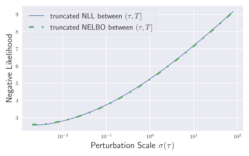
Figure 14: NELBO is uniformly close to NLL on CIFAR-10.

It now remains to show if the assumptions of Theorem 1 holds in practice. Figure 14 compares the NLL and NELBO curve of 𝐬𝜽fragmentssfragmentsθ\mathbf{s}_{\bm{\theta}_{\infty}}. Figure 14 shows that the equality condition of NLL and NELBO holds approximately on a wide range of time horizon, in practice.

Figure 14 is obtained from the EDM checkpoint (Karras et al., 2022). For the NLL and NELBO computation, we follow Kim et al. (2022a, b): we estimate the truncated NLL and NELBO for the purpose of thorough investigation throughout timescales. The truncated NLL and NELBO assumes that the score network is given only on (τ,T]fragments(τ,T](\tau,T] with τ𝜏\tau a truncation bound. Then, the truncated NLL is the right-hand-side of

𝔼𝐱0pr[logpg(𝐱0)]𝔼𝐱τprτ[logp𝜽,τ(𝐱τ)]+Rτ(𝜽),fragmentsEfragmentsx0similar-top𝑟[p𝑔(x0)]Efragmentsx𝜏similar-top𝑟𝜏[pfragmentsθ,τ(x𝜏)]R𝜏(θ),\displaystyle\mathbb{E}_{\mathbf{x}_{0}\sim p_{r}}[-\log{p_{g}(\mathbf{x}_{0})}]\leq\mathbb{E}_{\mathbf{x}_{\tau}\sim p_{r}^{\tau}}[-\log{p_{\bm{\theta},\tau}(\mathbf{x}_{\tau})}]+R_{\tau}(\bm{\theta}),

where Rτ(𝜽)=𝔼𝐱0pr[p0τ(𝐱τ|𝐱0)logp0τ(𝐱τ|𝐱0)p𝜽(𝐱0|𝐱τ)d𝐱τ]fragmentsR𝜏(θ)Efragmentsx0similar-top𝑟[pfragments0τ(x𝜏|x0)fragmentspfragments0τ(x𝜏|x0)fragmentsp𝜽(x0|x𝜏)dx𝜏]R_{\tau}(\bm{\theta})=\mathbb{E}_{\mathbf{x}_{0}\sim p_{r}}\big{[}\int p_{0\tau}(\mathbf{x}_{\tau}|\mathbf{x}_{0})\log{\frac{p_{0\tau}(\mathbf{x}_{\tau}|\mathbf{x}_{0})}{p_{\bm{\theta}}(\mathbf{x}_{0}|\mathbf{x}_{\tau})}}\mathop{}\!\mathrm{d}\mathbf{x}_{\tau}\big{]} and p𝜽,τfragmentspfragmentsθ,τp_{\bm{\theta},\tau} is the marginal density at τ𝜏\tau of the generative process. We evaluate p𝜽,τ(𝐱τ)fragmentspfragmentsθ,τ(x𝜏)p_{\bm{\theta},\tau}(\mathbf{x}_{\tau}) by solving the instantaneous change-of-variable formula

ddtlogp𝜽,t(𝐱t)=tr([𝐟(𝐱t,t)12g2(t)𝐱𝜽(𝐱t,t)])fragmentsfragmentsdfragmentsdtpfragmentsθ,t(x𝑡)tr([f(x𝑡,t)12g2(t)x𝜽(x𝑡,t)])\displaystyle\frac{\mathop{}\!\mathrm{d}}{\mathop{}\!\mathrm{d}t}\log{p_{\bm{\theta},t}(\mathbf{x}_{t})}=-\text{tr}\bigg{(}\nabla\Big{[}\mathbf{f}(\mathbf{x}_{t},t)-\frac{1}{2}g^{2}(t)\mathbf{x}_{\bm{\theta}}(\mathbf{x}_{t},t)\Big{]}\bigg{)}

from t=τfragmentstτt=\tau to T𝑇T, of which probability flow ODE is

d𝐱t=[𝐟(𝐱t,t)12g2(t)𝐬𝜽(𝐱t,t)]dt.fragmentsdx𝑡[f(x𝑡,t)12g2(t)s𝜽(x𝑡,t)]dt.\displaystyle\mathop{}\!\mathrm{d}\mathbf{x}_{t}=\bigg{[}\mathbf{f}(\mathbf{x}_{t},t)-\frac{1}{2}g^{2}(t)\mathbf{s}_{\bm{\theta}}(\mathbf{x}_{t},t)\bigg{]}\mathop{}\!\mathrm{d}t.

Analogously, we evaluate the truncated evidence lower bound as the right-hand-side of

([0,T])([τ,T])+Rτ(𝜽),fragmentsL([0,T])L([τ,T])R𝜏(θ),\displaystyle\mathcal{L}([0,T])\leq\mathcal{L}([\tau,T])+R_{\tau}(\bm{\theta}),

where

([τ,T])fragmentsL([τ,T])\displaystyle\mathcal{L}([\tau,T]) =12τT𝔼[g2(t)logp0t(𝐱t|𝐱0)𝐬𝜽(𝐱t,t)22g2(t)logp0t(𝐱t|𝐱0)222div(𝐟)]dt𝔼[logπ(𝐱T)].fragments12𝜏𝑇E[g2(t)pfragments0t(x𝑡|x0)s𝜽(x𝑡,t)22g2(t)pfragments0t(x𝑡|x0)222div(f)]dtE[π(x𝑇)].\displaystyle=\frac{1}{2}\int_{\tau}^{T}\mathbb{E}\Big{[}g^{2}(t)\|\nabla\log{p_{0t}(\mathbf{x}_{t}|\mathbf{x}_{0})}-\mathbf{s}_{\bm{\theta}}(\mathbf{x}_{t},t)\|_{2}^{2}-g^{2}(t)\|\nabla\log{p_{0t}(\mathbf{x}_{t}|\mathbf{x}_{0})}\|_{2}^{2}-2\text{div}(\mathbf{f})\Big{]}\mathop{}\!\mathrm{d}t-\mathbb{E}\big{[}\log{\pi(\mathbf{x}_{T})}\big{]}.

We utilize the importance sampling technique (for the integration with respect to t𝑡t in \mathcal{L}) to minimize the estimation variance of the evidence lower bound. To derive the closed-form importance-weighted time, first, observe that the EDM forward diffusion is given by σ2(t)=(σmin1/ρ+t(σmax1/ρσmin1/ρ))fragmentsσ2(t)(σfragmentsminfragments1ρt(σfragmentsmaxfragments1ρσfragmentsminfragments1ρ))\sigma^{2}(t)=(\sigma_{min}^{1/\rho}+t(\sigma_{max}^{1/\rho}-\sigma_{min}^{1/\rho})). Then, with the importance weight of g2(t)σ2(t)fragmentsg2(t)fragmentsσ2(t)\frac{g^{2}(t)}{\sigma^{2}(t)}, if we define F(t)=1Zτtg2(s)σ2(s)dsfragmentsF(t)1𝑍𝜏𝑡fragmentsg2(s)fragmentsσ2(s)dsF(t)=\frac{1}{Z}\int_{\tau}^{t}\frac{g^{2}(s)}{\sigma^{2}(s)}\mathop{}\!\mathrm{d}s to be the cumulative distribution function of the importance sampler, the importance-weighted time becomes t=F1(u)fragmentstFfragments1(u)t=F^{-1}(u) for uniformly sampled u𝑢u on [0,T]fragments[0,T][0,T].

Now, the antiderivative of the importance weight becomes

(t)fragmentsF(t)\displaystyle\mathcal{F}(t) =g2(t)σ2(t)dtfragmentsfragmentsg2(t)fragmentsσ2(t)dt\displaystyle=\int\frac{g^{2}(t)}{\sigma^{2}(t)}\mathop{}\!\mathrm{d}t
=2ρσmax1/ρσmin1/ρσmin1/ρ+t(σmax1/ρσmin1/ρ)dtfragments2ρfragmentsσfragmentsmaxfragments1ρσfragmentsminfragments1ρfragmentsσfragmentsminfragments1ρt(σfragmentsmaxfragments1ρσfragmentsminfragments1ρ)dt\displaystyle=\int 2\rho\frac{\sigma_{max}^{1/\rho}-\sigma_{min}^{1/\rho}}{\sigma_{min}^{1/\rho}+t(\sigma_{max}^{1/\rho}-\sigma_{min}^{1/\rho})}\mathop{}\!\mathrm{d}t
=2ρlog(σmin1/ρ+t(σmax1/ρσmin1/ρ)),fragments2ρ(σfragmentsminfragments1ρt(σfragmentsmaxfragments1ρσfragmentsminfragments1ρ)),\displaystyle=2\rho\log{(\sigma_{min}^{1/\rho}+t(\sigma_{max}^{1/\rho}-\sigma_{min}^{1/\rho}))},

and the normalizing constant becomes

Z𝑍\displaystyle Z =τTg2(t)σ2(t)dtfragments𝜏𝑇fragmentsg2(t)fragmentsσ2(t)dt\displaystyle=\int_{\tau}^{T}\frac{g^{2}(t)}{\sigma^{2}(t)}\mathop{}\!\mathrm{d}t
=(T)(τ)fragmentsF(T)F(τ)\displaystyle=\mathcal{F}(T)-\mathcal{F}(\tau)
=2ρlogσmin1/ρ+T(σmax1/ρσmin1/ρ)σmin1/ρ+τ(σmax1/ρσmin1/ρ).fragments2ρfragmentsσfragmentsminfragments1ρT(σfragmentsmaxfragments1ρσfragmentsminfragments1ρ)fragmentsσfragmentsminfragments1ρτ(σfragmentsmaxfragments1ρσfragmentsminfragments1ρ).\displaystyle=2\rho\log{\frac{\sigma_{min}^{1/\rho}+T(\sigma_{max}^{1/\rho}-\sigma_{min}^{1/\rho})}{\sigma_{min}^{1/\rho}+\tau(\sigma_{max}^{1/\rho}-\sigma_{min}^{1/\rho})}}.

Therefore, we have

t=F1(u)fragmentstFfragments1(u)\displaystyle t=F^{-1}(u)
u=F(t)=1Zτtg2(s)σ2(s)ds=1Z((t)(τ))fragmentsiffuF(t)1𝑍𝜏𝑡fragmentsg2(s)fragmentsσ2(s)ds1𝑍(F(t)F(τ))\displaystyle\iff u=F(t)=\frac{1}{Z}\int_{\tau}^{t}\frac{g^{2}(s)}{\sigma^{2}(s)}\mathop{}\!\mathrm{d}s=\frac{1}{Z}\big{(}\mathcal{F}(t)-\mathcal{F}(\tau)\big{)}
ulogσmin1/ρ+T(σmax1/ρσmin1/ρ)σmin1/ρ+τ(σmax1/ρσmin1/ρ)=logσmin1/ρ+t(σmax1/ρσmin1/ρ)σmin1/ρ+τ(σmax1/ρσmin1/ρ)fragmentsiffufragmentsσfragmentsminfragments1ρT(σfragmentsmaxfragments1ρσfragmentsminfragments1ρ)fragmentsσfragmentsminfragments1ρτ(σfragmentsmaxfragments1ρσfragmentsminfragments1ρ)fragmentsσfragmentsminfragments1ρt(σfragmentsmaxfragments1ρσfragmentsminfragments1ρ)fragmentsσfragmentsminfragments1ρτ(σfragmentsmaxfragments1ρσfragmentsminfragments1ρ)\displaystyle\iff u\log{\frac{\sigma_{min}^{1/\rho}+T(\sigma_{max}^{1/\rho}-\sigma_{min}^{1/\rho})}{\sigma_{min}^{1/\rho}+\tau(\sigma_{max}^{1/\rho}-\sigma_{min}^{1/\rho})}}=\log{\frac{\sigma_{min}^{1/\rho}+t(\sigma_{max}^{1/\rho}-\sigma_{min}^{1/\rho})}{\sigma_{min}^{1/\rho}+\tau(\sigma_{max}^{1/\rho}-\sigma_{min}^{1/\rho})}}
(σmin1/ρ+T(σmax1/ρσmin1/ρ)σmin1/ρ+τ(σmax1/ρσmin1/ρ))u=σmin1/ρ+t(σmax1/ρσmin1/ρ)σmin1/ρ+τ(σmax1/ρσmin1/ρ)fragmentsiff(fragmentsσfragmentsminfragments1ρT(σfragmentsmaxfragments1ρσfragmentsminfragments1ρ)fragmentsσfragmentsminfragments1ρτ(σfragmentsmaxfragments1ρσfragmentsminfragments1ρ))𝑢fragmentsσfragmentsminfragments1ρt(σfragmentsmaxfragments1ρσfragmentsminfragments1ρ)fragmentsσfragmentsminfragments1ρτ(σfragmentsmaxfragments1ρσfragmentsminfragments1ρ)\displaystyle\iff\bigg{(}\frac{\sigma_{min}^{1/\rho}+T(\sigma_{max}^{1/\rho}-\sigma_{min}^{1/\rho})}{\sigma_{min}^{1/\rho}+\tau(\sigma_{max}^{1/\rho}-\sigma_{min}^{1/\rho})}\bigg{)}^{u}=\frac{\sigma_{min}^{1/\rho}+t(\sigma_{max}^{1/\rho}-\sigma_{min}^{1/\rho})}{\sigma_{min}^{1/\rho}+\tau(\sigma_{max}^{1/\rho}-\sigma_{min}^{1/\rho})}
(σmin1/ρ+τ(σmax1/ρσmin1/ρ))(σmin1/ρ+T(σmax1/ρσmin1/ρ)σmin1/ρ+τ(σmax1/ρσmin1/ρ))u=σmin1/ρ+t(σmax1/ρσmin1/ρ)fragmentsiff(σfragmentsminfragments1ρτ(σfragmentsmaxfragments1ρσfragmentsminfragments1ρ))(fragmentsσfragmentsminfragments1ρT(σfragmentsmaxfragments1ρσfragmentsminfragments1ρ)fragmentsσfragmentsminfragments1ρτ(σfragmentsmaxfragments1ρσfragmentsminfragments1ρ))𝑢σfragmentsminfragments1ρt(σfragmentsmaxfragments1ρσfragmentsminfragments1ρ)\displaystyle\iff\big{(}\sigma_{min}^{1/\rho}+\tau(\sigma_{max}^{1/\rho}-\sigma_{min}^{1/\rho})\big{)}\bigg{(}\frac{\sigma_{min}^{1/\rho}+T(\sigma_{max}^{1/\rho}-\sigma_{min}^{1/\rho})}{\sigma_{min}^{1/\rho}+\tau(\sigma_{max}^{1/\rho}-\sigma_{min}^{1/\rho})}\bigg{)}^{u}=\sigma_{min}^{1/\rho}+t(\sigma_{max}^{1/\rho}-\sigma_{min}^{1/\rho})
t=((σmin1/ρ+τ(σmax1/ρσmin1/ρ))(σmin1/ρ+T(σmax1/ρσmin1/ρ)σmin1/ρ+τ(σmax1/ρσmin1/ρ))uσmin1/ρ)/(σmax1/ρσmin1/ρ).fragmentsifft((σfragmentsminfragments1ρτ(σfragmentsmaxfragments1ρσfragmentsminfragments1ρ))(fragmentsσfragmentsminfragments1ρT(σfragmentsmaxfragments1ρσfragmentsminfragments1ρ)fragmentsσfragmentsminfragments1ρτ(σfragmentsmaxfragments1ρσfragmentsminfragments1ρ))𝑢σfragmentsminfragments1ρ)(σfragmentsmaxfragments1ρσfragmentsminfragments1ρ).\displaystyle\iff t=\bigg{(}\big{(}\sigma_{min}^{1/\rho}+\tau(\sigma_{max}^{1/\rho}-\sigma_{min}^{1/\rho})\big{)}\bigg{(}\frac{\sigma_{min}^{1/\rho}+T(\sigma_{max}^{1/\rho}-\sigma_{min}^{1/\rho})}{\sigma_{min}^{1/\rho}+\tau(\sigma_{max}^{1/\rho}-\sigma_{min}^{1/\rho})}\bigg{)}^{u}-\sigma_{min}^{1/\rho}\bigg{)}\bigg{/}(\sigma_{max}^{1/\rho}-\sigma_{min}^{1/\rho}).

A.4 Why p𝜽tfragmentsp𝜽𝑡p_{\bm{\theta}}^{t} is defined as a forward marginal rather than a generative marginal

Unintuitively, we define p𝜽tfragmentsp𝜽𝑡p_{\bm{\theta}}^{t} as a forward-time marginal density rather than a reverse-time generative marginal. We design p𝜽tfragmentsp𝜽𝑡p_{\bm{\theta}}^{t} as a forward-time marginal by two reasons. First, it saves memory. If it was the reverse-time generative marginal, the generated dataset 𝒢𝒢\mathcal{G} should contain the whole sample trajectories to optimize the time-embedded discriminator, and this could be prohibitive when we run 1000fragmentssimilar-to1000\sim 1000 steps to generate a sample. Instead, if we use the forward-time marginal, we could only save the final sample as 𝒢𝒢\mathcal{G}, and we optimize the discriminator by diffusing it with arbitrary diffusion time with arbitrary diffusion noise. Here comes the second advantage: as we could update the discriminator with arbitrary diffusion noise, it attains the data augmentation effect in training the discriminator network, and it could prevent the overfitting issue at large time. On the other hand, if it was the generative marginal, the discriminator guidance needs more sample data to prevent overfitting.
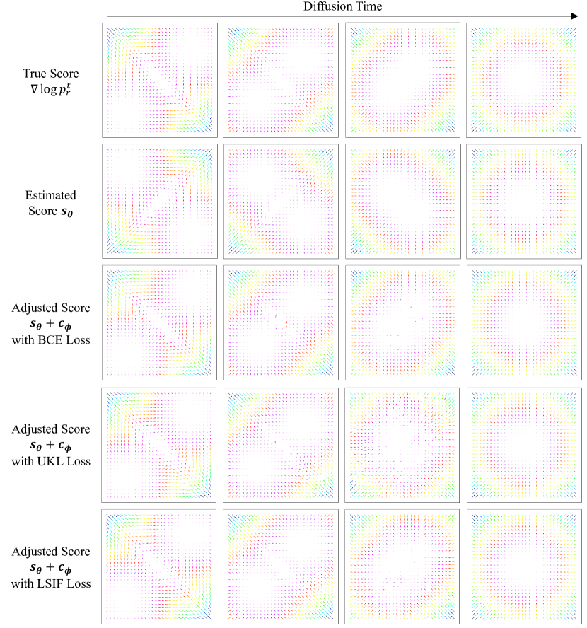
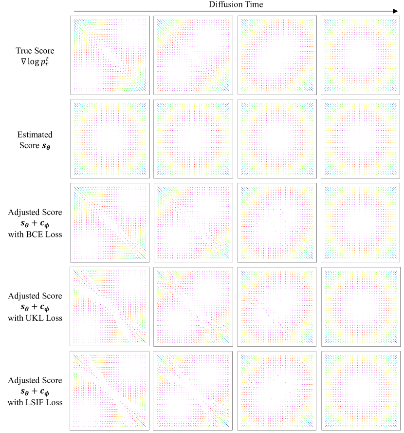
Refer to caption
Figure 15: A 2-dimentionsal toy case with a bimodal Gaussian data distribution. In this experiment, we visualize the adjusted scores for BKL/UKL/LSIF losses under the assumption that the estimated score is misleadingly capturing the location of bimodalities.
Refer to caption
Figure 16: A 2-dimentionsal toy case with a bimodal Gaussian data distribution. In this experiment, we visualize the adjusted scores for BKL/UKL/LSIF losses under the assumption that the estimated score is completely blind to the data distribution, which means that the estimated score 𝐬𝜽fragmentss𝜽\mathbf{s}_{\bm{\theta}} is simply a score function of a standard Gaussian distribution.
Refer to caption
(a) FID by Discriminator Training
Refer to caption
(b) Loss Contribution
Figure 17: Study of EDM on CIFAR-10 with respect to Bregman divergences. (a) illustrates how sample quality is improved by discriminator training with various loss functions, and (b) shows the mechanism of such different FID.

Appendix B More on Bregman Divergences

The most general framework for learning the density-ratio prtp𝜽tfragmentsp𝑟𝑡fragmentsp𝜽𝑡\frac{p_{r}^{t}}{p_{\bm{\theta}}^{t}} is using the Bregman divergence (Sugiyama et al., 2012). In this section, we investigate the effect of representative Bregman divergences. To begin with, let us define the Bregman divergence in an abstract form. Suppose r(𝐱)=pnu(𝐱)pde(𝐱)fragmentsr(x)fragmentspfragmentsnu(x)fragmentspfragmentsde(x)r^{*}(\mathbf{x})=\frac{p_{nu}(\mathbf{x})}{p_{de}(\mathbf{x})} be the target density-ratio to be estimated with rϕfragmentsrbold-italic-ϕr_{\bm{\phi}}, parametrized by ϕbold-italic-ϕ\bm{\phi}. Then,

Dh(rrϕ)fragmentsD(rrbold-italic-ϕ)\displaystyle D_{h}(r^{*}\|r_{\bm{\phi}}) =pde(𝐱)Bh(r(𝐱)rϕ(𝐱))d𝐱fragmentspfragmentsde(x)B(r(x)rbold-italic-ϕ(x))dx\displaystyle=\int p_{de}(\mathbf{x})B_{h}(r^{*}(\mathbf{x})\|r_{\bm{\phi}}(\mathbf{x}))\mathop{}\!\mathrm{d}\mathbf{x}
=pde(𝐱)(h(r(𝐱))h(rϕ(𝐱))h(rϕ(𝐱))(r(𝐱)rϕ(𝐱)))d𝐱,fragmentspfragmentsde(x)(h(r(x))h(rbold-italic-ϕ(x))h(rbold-italic-ϕ(x))(r(x)rbold-italic-ϕ(x)))dx,\displaystyle=\int p_{de}(\mathbf{x})\Big{(}h\big{(}r^{*}(\mathbf{x})\big{)}-h\big{(}r_{\bm{\phi}}(\mathbf{x})\big{)}-\partial h\big{(}r_{\bm{\phi}}(\mathbf{x})\big{)}\big{(}r^{*}(\mathbf{x})-r_{\bm{\phi}}(\mathbf{x})\big{)}\Big{)}\mathop{}\!\mathrm{d}\mathbf{x},

where BhfragmentsBB_{h} is the data-level Bregman divergence. For a twice continuously differentiable convex function hh with a bounded derivative hfragmentsh\partial h, the Bregman divergence quantifies the discrepancy between two density-ratios. Subtracting a constant term pde(𝐱)h(r(𝐱))dxfragmentspfragmentsde(x)h(r(x))dx\int p_{de}(\mathbf{x})h(r^{*}(\mathbf{x}))\mathop{}\!\mathrm{d}x, we obtain (up to a constant)

Dh(rrϕ)=pde(𝐱)[h(rϕ(𝐱))rϕ(𝐱)h(rϕ(𝐱))]d𝐱pnu(𝐱)[h(rϕ(𝐱))]d𝐱.fragmentsD(rrbold-italic-ϕ)pfragmentsde(x)[h(rbold-italic-ϕ(x))rbold-italic-ϕ(x)h(rbold-italic-ϕ(x))]dxpfragmentsnu(x)[h(rbold-italic-ϕ(x))]dx.\displaystyle D_{h}(r^{*}\|r_{\bm{\phi}})=\int p_{de}(\mathbf{x})\Big{[}\partial h\big{(}r_{\bm{\phi}}(\mathbf{x})\big{)}r_{\bm{\phi}}(\mathbf{x})-h\big{(}r_{\bm{\phi}}(\mathbf{x})\big{)}\Big{]}\mathop{}\!\mathrm{d}\mathbf{x}-\int p_{nu}(\mathbf{x})\Big{[}\partial h\big{(}r_{\bm{\phi}}(\mathbf{x})\big{)}\Big{]}\mathop{}\!\mathrm{d}\mathbf{x}.

A few non-exhaustive examples of the Bregman divergence are Least-Squared Importance Fitting (LSIF) (Kanamori et al., 2009), Binary Cross Entropy (BCE) (Hastie et al., 2009), and Kullback-Leibler Importance Estimation Procedure (KLIEP) (Nguyen et al., 2010). LSIF is equivalent to

BDfLSIF(rrϕ)fragmentsBDfragmentsffragmentsLSIF(rrbold-italic-ϕ)\displaystyle BD_{f_{LSIF}}(r^{*}\|r_{\bm{\phi}}) =12pde(𝐱)(r(𝐱)rϕ(𝐱))2d𝐱fragments12pfragmentsde(x)(r(x)rbold-italic-ϕ(x))2dx\displaystyle=\frac{1}{2}\int p_{de}(\mathbf{x})\big{(}r^{*}(\mathbf{x})-r_{\bm{\phi}}(\mathbf{x})\big{)}^{2}\mathop{}\!\mathrm{d}\mathbf{x}
=12pde(𝐱)rϕ2(𝐱)d𝐱pnu(𝐱)rϕ(𝐱)d𝐱,fragments12pfragmentsde(x)rbold-italic-ϕ2(x)dxpfragmentsnu(x)rbold-italic-ϕ(x)dx,\displaystyle=\frac{1}{2}\int p_{de}(\mathbf{x})r_{\bm{\phi}}^{2}(\mathbf{x})\mathop{}\!\mathrm{d}\mathbf{x}-\int p_{nu}(\mathbf{x})r_{\bm{\phi}}(\mathbf{x})\mathop{}\!\mathrm{d}\mathbf{x},

with hLSIF(r)=(r1)2/2fragmentshfragmentsLSIF(r)(r1)22h_{LSIF}(r)=(r-1)^{2}/2. BCE is also widely denoted as Binary Kullback-Leibler (BKL), and is defined with hBKL(r)=rlogr(1+r)log(1+r)fragmentshfragmentsBKL(r)rr(1r)(1r)h_{BKL}(r)=r\log{r}-(1+r)\log{(1+r)}. KLIEP is also known as the Unbounded Kullback-Leibler (UKL) with hUKL(r)=rlogrrfragmentshfragmentsUKL(r)rrrh_{UKL}(r)=r\log{r}-r, and is a Lagrangian of the constrained optimization problem of

DKL(pnupnu,ϕ) subject to pnu,ϕ(𝐱)d𝐱=1,fragmentsDfragmentsKL(pfragmentsnupfragmentsnu,ϕ) subject to pfragmentsnu,ϕ(x)dx1,\displaystyle D_{KL}(p_{nu}\|p_{nu,\bm{\phi}})\text{ subject to }\int p_{nu,\bm{\phi}}(\mathbf{x})\mathop{}\!\mathrm{d}\mathbf{x}=1,

where pnu,ϕ(𝐱):=pde(𝐱)rϕ(𝐱)fragmentspfragmentsnu,ϕ(x)assignpfragmentsde(x)rbold-italic-ϕ(x)p_{nu,\bm{\phi}}(\mathbf{x}):=p_{de}(\mathbf{x})r_{\bm{\phi}}(\mathbf{x}). The UKL Bregman divergence is defined as the Lagrangian of the above problem by

BDfUKL(rrϕ)=pde(𝐱)rϕ(𝐱)d𝐱pnu(𝐱)logrϕ(𝐱)d𝐱.fragmentsBDfragmentsffragmentsUKL(rrbold-italic-ϕ)pfragmentsde(x)rbold-italic-ϕ(x)dxpfragmentsnu(x)rbold-italic-ϕ(x)dx.\displaystyle BD_{f_{UKL}}(r^{*}\|r_{\bm{\phi}})=\int p_{de}(\mathbf{x})r_{\bm{\phi}}(\mathbf{x})\mathop{}\!\mathrm{d}\mathbf{x}-\int p_{nu}(\mathbf{x})\log{r_{\bm{\phi}}(\mathbf{x})}\mathop{}\!\mathrm{d}\mathbf{x}.

Now, we consider the time-dependent Bregman divergence to train the discriminator network. The time-dependent Bregman divergence is defined by

λ(t)Dh(prt()p𝜽t()1dϕ(,t)dϕ(,t))dt,fragmentsλ(t)D(fragmentsp𝑟𝑡()fragmentsp𝜽𝑡()fragments1dbold-italic-ϕ(,t)fragmentsdbold-italic-ϕ(,t))dt,\displaystyle\int\lambda(t)D_{h}\bigg{(}\frac{p_{r}^{t}(\cdot)}{p_{\bm{\theta}}^{t}(\cdot)}\Big{\|}\frac{1-d_{\bm{\phi}}(\cdot,t)}{d_{\bm{\phi}}(\cdot,t)}\bigg{)}\mathop{}\!\mathrm{d}t,

where λ(t)fragmentsλ(t)\lambda(t) is a time-weighting function. We train the discriminator network with this time-dependent Bregman divergence of LSIF, BCE, and UKL. In a toy 2-dimensional case, Figures 16 and 15 visualizes the adjusted score by discriminators trained by aforementioned Bregman divergences: Figure 16 for the case where the estimated score is completely blind to the data score, and Figure 15 for the case where the estimated score is confusing on the exact location of bi-modalities of the data distribution. Figures 16 and 15 illustrate that BCE estimates the correction term 𝐜𝜽fragmentsc𝜽\mathbf{c}_{\bm{\theta}} most robust.

Refer to caption
Figure 18: Study of wtDGfragmentsw𝑡fragmentsDGw_{t}^{DG} for various Bregman divergences on CIFAR-10.

Figure 17-(a) shows that the listed divergences have distinctive characteristics in sample quality. Similar to the 2-dimensional case, BCE performs the best. Figure 17-(b) illustrates why such a behavioral difference occurs. We visualize the (normalized) cumulative loss to the perturbation scale. For the noise matching, most loss contribution is on the range of small diffusion scale (Kim et al., 2022b). On the contrary, BCE is qualitatively different from the score loss: most of loss is concentrated on the range of large diffusion scale, and it would be presumably the reason for the arguments in Section 6. Figure 17-(b) shows that LSIF is similar to the noise matching loss. For the UKL loss, we do not plot the cumulative loss because the loss is neither strictly positive nor strictly negative for every diffusion scale.

Figure 18 conducts the ablation study of wtDGfragmentsw𝑡fragmentsDGw_{t}^{DG} for various Bregman divergences on CIFAR-10. It illustrates that BCE loss performs the best but UKL loss is the most robust one.

Appendix C Details on Image-to-Image Translation
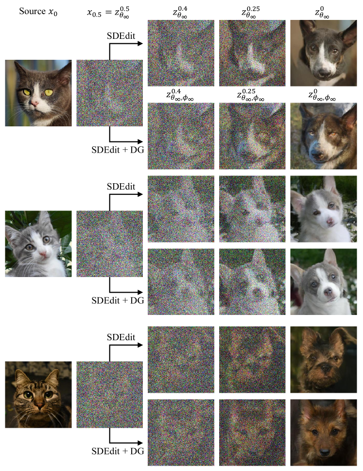
Refer to caption
Figure 19: Step-by-step denoising illustration of image-to-image translation.

Figure 19 illustrates the step-by-step denoising process of I2I translation task. Suppose 𝐱0𝒮fragmentsx0similar-toS\mathbf{x}_{0}\sim\mathcal{S} is the source image, and 𝐲0𝒯fragmentsy0similar-toT\mathbf{y}_{0}\sim\mathcal{T} is the target image. Then, following SDEdit (Meng et al., 2021), we start denoising from 𝐱τfragmentsx𝜏\mathbf{x}_{\tau} with

d𝐲t=[𝐟(𝐲t,t)g2(t)𝐬𝜽(𝐲t,t)]dt¯+g(t)d𝐰¯t,fragmentsdy𝑡[f(y𝑡,t)g2(t)s𝜽(y𝑡,t)]d¯𝑡g(t)d¯𝐰𝑡,\displaystyle\mathop{}\!\mathrm{d}\mathbf{y}_{t}=[\mathbf{f}(\mathbf{y}_{t},t)-g^{2}(t)\mathbf{s}_{\bm{\theta}}(\mathbf{y}_{t},t)]\mathop{}\!\mathrm{d}\bar{t}+g(t)\mathop{}\!\mathrm{d}\mathbf{\bar{w}}_{t},

where 𝐬𝜽(𝐲t,t)fragmentss𝜽(y𝑡,t)\mathbf{s}_{\bm{\theta}}(\mathbf{y}_{t},t) is the score network trained on the target domain. Suppose we define 𝐳𝜽tfragmentsz𝜽𝑡\mathbf{z}_{\bm{\theta}}^{t} be the random variable of the solution process: 𝐳𝜽tmid=𝐱tmidfragmentsz𝜽fragmentstfragmentsmidxfragmentstfragmentsmid\mathbf{z}_{\bm{\theta}}^{t_{mid}}=\mathbf{x}_{t_{mid}} is the starting variable and 𝐳𝜽0fragmentsz𝜽0\mathbf{z}_{\bm{\theta}}^{0} is the translated variable. Suppose q𝜽tfragmentsq𝜽𝑡q_{\bm{\theta}}^{t} be the probability distribution of 𝐳𝜽tfragmentsz𝜽𝑡\mathbf{z}_{\bm{\theta}}^{t}, p𝜽=q𝜽0fragmentsp𝜽q𝜽0p_{\bm{\theta}}=q_{\bm{\theta}}^{0} be the probability distribution of 𝐳𝜽0fragmentsz𝜽0\mathbf{z}_{\bm{\theta}}^{0}, and p𝜽tfragmentsp𝜽𝑡p_{\bm{\theta}}^{t} be the probability distribution of the diffused variable by the forward SDE, starting from 𝐳𝜽0fragmentsz𝜽0\mathbf{z}_{\bm{\theta}}^{0}. For the discriminator training, we sample 𝐳tαp𝒮t(𝐳t)+(1α)p𝜽t(𝐳t)fragmentsz𝑡similar-toαp𝒮𝑡(z𝑡)(1α)p𝜽𝑡(z𝑡)\mathbf{z}_{t}\sim\alpha p_{\mathcal{S}}^{t}(\mathbf{z}_{t})+(1-\alpha)p_{\bm{\theta}}^{t}(\mathbf{z}_{t}) for the fake data and 𝐲tp𝒯t(𝐲t)fragmentsy𝑡similar-top𝒯𝑡(y𝑡)\mathbf{y}_{t}\sim p_{\mathcal{T}}^{t}(\mathbf{y}_{t}) for the real data. Then, our discriminator guidance becomes

d𝐲t=[𝐟(𝐲t,t)g2(t)(𝐬𝜽(𝐲t,t)+logp𝒯t(𝐲t)αp𝒮t(𝐲t)+(1α)p𝜽t(𝐲t))]dt¯+g(t)d𝐰¯t.fragmentsdy𝑡[f(y𝑡,t)g2(t)(s𝜽(y𝑡,t)fragmentsp𝒯𝑡(y𝑡)fragmentsαp𝒮𝑡(y𝑡)(1α)p𝜽𝑡(y𝑡))]d¯𝑡g(t)d¯𝐰𝑡.\displaystyle\mathop{}\!\mathrm{d}\mathbf{y}_{t}=\bigg{[}\mathbf{f}(\mathbf{y}_{t},t)-g^{2}(t)\Big{(}\mathbf{s}_{\bm{\theta}}(\mathbf{y}_{t},t)+\nabla\log{\frac{p_{\mathcal{T}}^{t}(\mathbf{y}_{t})}{\alpha p_{\mathcal{S}}^{t}(\mathbf{y}_{t})+(1-\alpha)p_{\bm{\theta}}^{t}(\mathbf{y}_{t})}}\Big{)}\bigg{]}\mathop{}\!\mathrm{d}\bar{t}+g(t)\mathop{}\!\mathrm{d}\mathbf{\bar{w}}_{t}.

When ttmidfragmentsttfragmentsmidt\approx t_{mid}, we have p𝒮t(𝐳t)p𝜽t(𝐳t)fragmentsp𝒮𝑡(z𝑡)much-greater-thanp𝜽𝑡(z𝑡)p_{\mathcal{S}}^{t}(\mathbf{z}_{t})\gg p_{\bm{\theta}}^{t}(\mathbf{z}_{t}) for 𝐳tq𝜽tfragmentsz𝑡similar-toq𝜽𝑡\mathbf{z}_{t}\sim q_{\bm{\theta}}^{t} and the adjusted generative process is approximately

d𝐲t[𝐟(𝐲t,t)g2(t)(𝐬𝜽(𝐲t,t)+logp𝒯t(𝐲t)p𝒮t(𝐲t))]dt¯+g(t)d𝐰¯t,fragmentsdy𝑡[f(y𝑡,t)g2(t)(s𝜽(y𝑡,t)fragmentsp𝒯𝑡(y𝑡)fragmentsp𝒮𝑡(y𝑡))]d¯𝑡g(t)d¯𝐰𝑡,\displaystyle\mathop{}\!\mathrm{d}\mathbf{y}_{t}\approx\bigg{[}\mathbf{f}(\mathbf{y}_{t},t)-g^{2}(t)\Big{(}\mathbf{s}_{\bm{\theta}}(\mathbf{y}_{t},t)+\nabla\log{\frac{p_{\mathcal{T}}^{t}(\mathbf{y}_{t})}{p_{\mathcal{S}}^{t}(\mathbf{y}_{t})}}\Big{)}\bigg{]}\mathop{}\!\mathrm{d}\bar{t}+g(t)\mathop{}\!\mathrm{d}\mathbf{\bar{w}}_{t},

so the discriminator guidance gives a direct signal to avoid from p𝒮tfragmentsp𝒮𝑡p_{\mathcal{S}}^{t} when ttmidfragmentsttfragmentsmidt\approx t_{mid}. When t0fragmentst0t\approx 0, we have p𝒮t(𝐳t)p𝜽t(𝐳t)fragmentsp𝒮𝑡(z𝑡)much-less-thanp𝜽𝑡(z𝑡)p_{\mathcal{S}}^{t}(\mathbf{z}_{t})\ll p_{\bm{\theta}}^{t}(\mathbf{z}_{t}) for 𝐳tq𝜽tfragmentsz𝑡similar-toq𝜽𝑡\mathbf{z}_{t}\sim q_{\bm{\theta}}^{t} and the adjusted generative process is approximately

d𝐲t[𝐟(𝐲t,t)g2(t)(𝐬𝜽(𝐲t,t)+logp𝒯t(𝐲t)p𝜽t(𝐲t))]dt¯+g(t)d𝐰¯t,fragmentsdy𝑡[f(y𝑡,t)g2(t)(s𝜽(y𝑡,t)fragmentsp𝒯𝑡(y𝑡)fragmentsp𝜽𝑡(y𝑡))]d¯𝑡g(t)d¯𝐰𝑡,\displaystyle\mathop{}\!\mathrm{d}\mathbf{y}_{t}\approx\bigg{[}\mathbf{f}(\mathbf{y}_{t},t)-g^{2}(t)\Big{(}\mathbf{s}_{\bm{\theta}}(\mathbf{y}_{t},t)+\nabla\log{\frac{p_{\mathcal{T}}^{t}(\mathbf{y}_{t})}{p_{\bm{\theta}}^{t}(\mathbf{y}_{t})}}\Big{)}\bigg{]}\mathop{}\!\mathrm{d}\bar{t}+g(t)\mathop{}\!\mathrm{d}\mathbf{\bar{w}}_{t},

and the discriminator is guiding the sample denoising toward the desired destination density p𝒯tfragmentsp𝒯𝑡p_{\mathcal{T}}^{t}, rather than the original destination density p𝜽tfragmentsp𝜽𝑡p_{\bm{\theta}}^{t}.

Refer to caption
Figure 20: The discriminator guidance swifts the sweet spot to the range of small t0fragmentst0t_{0}.

By applying the discriminator guidance, more realistic samples are generated with relatively small tmidfragmentstfragmentsmidt_{mid}, compared to SDEdit, so we could lift the sweet spot of the image-to-image translation to a range of small tmidfragmentstfragmentsmidt_{mid} as in Figure 20.

Appendix D Experimental Details

D.1 Training and Sampling Details

Table 8: Training and sampling configurations.
CIFAR-10 CelebA FFHQ ImageNet256
LSGM-G++ EDM-G++ Soft Truncation-G++ EDM-G++ ADM-G++ DiT-G++
Pre-trained Score Network
Model LSGM EDM EDM Soft Truncation EDM ADM DiT
Class condition
Discriminator Training
SDE LVP LVP LVP CVP CVP LVP LVP
Class condition
Time sampling Importance Importance Importance Importance Importance Importance Importance
λ𝜆\lambda g2σ2fragmentsg2fragmentsσ2\frac{g^{2}}{\sigma^{2}} g2σ2fragmentsg2fragmentsσ2\frac{g^{2}}{\sigma^{2}} g2σ2fragmentsg2fragmentsσ2\frac{g^{2}}{\sigma^{2}} g2σ2fragmentsg2fragmentsσ2\frac{g^{2}}{\sigma^{2}} g2σ2fragmentsg2fragmentsσ2\frac{g^{2}}{\sigma^{2}} g2σ2fragmentsg2fragmentsσ2\frac{g^{2}}{\sigma^{2}} g2σ2fragmentsg2fragmentsσ2\frac{g^{2}}{\sigma^{2}}
Minimum diffusion time 0.01 105fragments10fragments510^{-5} 105fragments10fragments510^{-5} 105fragments10fragments510^{-5} 105fragments10fragments510^{-5} 105fragments10fragments510^{-5} 105fragments10fragments510^{-5}
EMA
Batch size 128 128 128 128 128 512 512
#𝒟fragments#D\#\mathcal{D} 50,000 50,000 50,000 10,000 60,000 1,281,167 1,281,167
#𝒢fragments#G\#\mathcal{G} 50,000 25,000 50,000 10,000 60,000 400,000 1,281,167
##\# Epochs 280 60 250 150 250 10 7
GPUs 1x V100 1x V100 1x V100 1x V100 1x V100 1x A100 1x A100
Pre-trained Classifier
Model No classifier ADM ADM ADM ADM ADM ADM
Input shape (data dimension) (B,32,32,3) (B,32,32,3) (B,64,64,3) (B,64,64,3) (B,256,256,3) (B,32,32,4)
Output shape (latent dimension) (B,8,8,512) (B,8,8,512) (B,8,8,512) (B,8,8,512) (B,8,8,512) (B,8,8,384)
Shallow U-Net Architecture
Input shape (latent dimension) (B,16,16,180) (B,8,8,512) (B,8,8,512) (B,8,8,512) (B,8,8,512) (B,8,8,512) (B,8,8,384)
Output shape (B,1) (B,1) (B,1) (B,1) (B,1) (B,1) (B,1)
Minimum value of discriminator (clip) 105fragments10fragments510^{-5} 0 0 0 0 105fragments10fragments510^{-5} 105fragments10fragments510^{-5}
Maximum value of discriminator (clip) 1105fragments110fragments51-10^{-5} 1 1 1 1 1105fragments110fragments51-10^{-5} 105fragments10fragments510^{-5}
Class condition
##\# Resnet blocks 5 4 4 6 6 4 4
##\# Attention blocks 3 3 3 5 5 3 3
Attention resolutions 16, 8 8 8 8 8 8 8
Model channel 128 128 128 128 128 128 128
Channel multiplier (1,2) 1 1 1 1 1 1
Sampling
SDE LVP WVE WVE LVP WVE LVP LVP
Class condition
Minimum value of discriminator (clip) 103fragments10fragments310^{-3} 105fragments10fragments510^{-5} 105fragments10fragments510^{-5} 105fragments10fragments510^{-5} 105fragments10fragments510^{-5} 105fragments10fragments510^{-5} 105fragments10fragments510^{-5}
Maximum value of discriminator (clip) 1103fragments110fragments31-10^{-3} 1105fragments110fragments51-10^{-5} 1105fragments110fragments51-10^{-5} 1105fragments110fragments51-10^{-5} 1105fragments110fragments51-10^{-5} 1105fragments110fragments51-10^{-5} 105fragments10fragments510^{-5}
Solver PFODE PFODE PFODE PFODE PFODE DDPM DDPM
Solver accuracy of 𝐬𝜽fragmentss𝜽\mathbf{s}_{\bm{\theta}} 1stfragments1st1^{\text{st}}-order 2ndfragments2nd2^{\text{nd}}-order 2ndfragments2nd2^{\text{nd}}-order 1stfragments1st1^{\text{st}}-order 2ndfragments2nd2^{\text{nd}}-order 1stfragments1st1^{\text{st}}-order 1stfragments1st1^{\text{st}}-order
Solver type of 𝐬𝜽fragmentss𝜽\mathbf{s}_{\bm{\theta}} RK45 Heun Heun RK45 Heun Euler (DDPM) Euler (DDPM)
Solver accuracy of 𝐜ϕfragmentscbold-italic-ϕ\mathbf{c}_{\bm{\phi}} 1stfragments1st1^{\text{st}}-order 1stfragments1st1^{\text{st}}-order 1stfragments1st1^{\text{st}}-order 1stfragments1st1^{\text{st}}-order 1stfragments1st1^{\text{st}}-order 1stfragments1st1^{\text{st}}-order 1stfragments1st1^{\text{st}}-order
Solver type of 𝐜ϕfragmentscbold-italic-ϕ\mathbf{c}_{\bm{\phi}} RK45 Euler Euler RK45 Euler Euler Euler
tmidfragmentstfragmentsmidt_{mid} 0.1 0.01 0.01 0.01 0.01 0.1 0.1
NFE 138 35 35 131 71 250 250
Classifier Guidance
EDS
wtCGfragmentsw𝑡fragmentsCGw_{t}^{CG} 0 0 0 0 0 Adaptive Adaptive
wtDGfragmentsw𝑡fragmentsDGw_{t}^{DG} 2 2 Adaptive Adaptive Adaptive Adaptive 1
Refer to caption
Figure 21: Ablation of wtDGfragmentsw𝑡fragmentsDGw_{t}^{DG} in LSGM-G++ on CIFAR-10.

Table 8 presents the experimental configuration for Tables 5.1, 5.1, and 5.2. Except for ImageNet 256x256, we solve the Probability-Flow ODE (PFODE) (Song et al., 2020b) for sampling. We use the adjusted PFODE

d𝐱tdt=𝐟(𝐱t,t)12g2(t)(𝐬𝜽+wtDG𝐜ϕ)(𝐱t,t)fragmentsfragmentsdx𝑡fragmentsdtf(x𝑡,t)12g2(t)(sfragmentsθw𝑡fragmentsDGcfragmentsϕ)(x𝑡,t)\displaystyle\frac{\mathop{}\!\mathrm{d}\mathbf{x}_{t}}{\mathop{}\!\mathrm{d}t}=\mathbf{f}(\mathbf{x}_{t},t)-\frac{1}{2}g^{2}(t)(\mathbf{s}_{\bm{\theta}_{\infty}}+w_{t}^{DG}\mathbf{c}_{\bm{\phi}_{\infty}})(\mathbf{x}_{t},t)

on t[tmid,T]fragmentst[tfragmentsmid,T]t\in[t_{mid},T] and the unadjusted PFODE

d𝐱tdt=𝐟(𝐱t,t)12g2(t)𝐬𝜽(𝐱t,t)fragmentsfragmentsdx𝑡fragmentsdtf(x𝑡,t)12g2(t)sfragmentsθ(x𝑡,t)\displaystyle\frac{\mathop{}\!\mathrm{d}\mathbf{x}_{t}}{\mathop{}\!\mathrm{d}t}=\mathbf{f}(\mathbf{x}_{t},t)-\frac{1}{2}g^{2}(t)\mathbf{s}_{\bm{\theta}_{\infty}}(\mathbf{x}_{t},t)

on t[0,tmid]fragmentst[0,tfragmentsmid]t\in[0,t_{mid}].

For LSGM-G++, we borrow the pre-trained CIFAR-10 checkpoint of LSGM with best FID (Vahdat et al., 2021) at https://github.com/NVlabs/LSGM. We do not use any of the pre-trained classifier for this latent-diffusion model, and we train a discriminator from scratch. We solve the unadjusted/adjusted PFODEs with explicit Runge-Kutta solver of order 5(4) (Dormand & Prince, 1980). We find wtDG=2fragmentsw𝑡fragmentsDG2w_{t}^{DG}=2 works the best in practice and report the value in Table 5.1. Figure 21 presents the ablation study on DG weight.
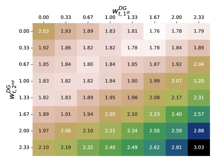
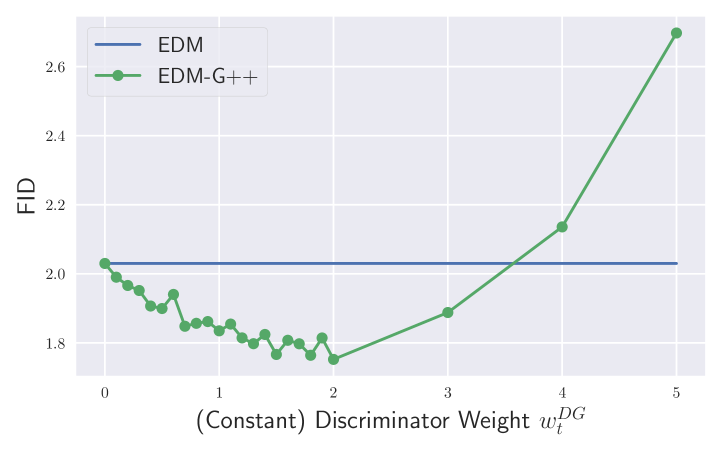
Refer to caption
(a) Ablation of wt,1stDGfragmentswfragmentst,1stfragmentsDGw_{t,1^{\text{st}}}^{DG} and wt,2ndDGfragmentswfragmentst,2ndfragmentsDGw_{t,2^{\text{nd}}}^{DG}
Refer to caption
(b) Detailed ablation of wt,1stDGfragmentswfragmentst,1stfragmentsDGw_{t,1^{\text{st}}}^{DG}
Figure 22: Study of Heun solver for EDM on unconditional CIFAR-10.

For EDM-G++, we experiment with unconditional and conditional CIFAR-10, as well as FFHQ 64x64. We use the pre-trained score model of EDM (Karras et al., 2022) at https://github.com/NVlabs/edm. For the classifier, we borrow a pre-trained classifier from ADM (Dhariwal & Nichol, 2021) at https://github.com/openai/guided-diffusion on 64x64 FFHQ, and we train a 32x32 classifier (and freeze it at discriminator training phase) for CIFAR-10 experiment. We use the ImageNet dataset (Russakovsky et al., 2015) to train the 32x32 classifier. We follow the identical setting of Dhariwal & Nichol (2021) to train the 32x32 classifier, except the dataset resolution. We solve the unadjusted/adjusted PFODEs with a Heun solver (Ascher & Petzold, 1998) with pre-designated timesteps that is determined by NFE. As the Heun solver is a 2ndnd{}^{\text{nd}}-order numerical solver, we divide the DG weight wtDGfragmentsw𝑡fragmentsDGw_{t}^{DG} into wt,1stDGfragmentswfragmentst,1stfragmentsDGw_{t,1^{\text{st}}}^{DG} and tt,2ndDGfragmentstfragmentst,2ndfragmentsDGt_{t,2^{\text{nd}}}^{DG}, where wt,1stDGfragmentswfragmentst,1stfragmentsDGw_{t,1^{\text{st}}}^{DG} is for the 1stfragments1st1^{\text{st}}-order and tt,2ndDGfragmentstfragmentst,2ndfragmentsDGt_{t,2^{\text{nd}}}^{DG} is for the 2ndfragments2nd2^{\text{nd}}-order. For denoising, we construct an intermediate state

𝐱~tΔt=𝐱tΔt[f(𝐱t,t)12g2(t)(𝐬𝜽+wt,1stDG𝐜ϕ)(𝐱t,t)].fragments~𝐱fragmentstΔtx𝑡Δt[f(x𝑡,t)12g2(t)(sfragmentsθwfragmentst,1stfragmentsDGcfragmentsϕ)(x𝑡,t)].\displaystyle\mathbf{\tilde{x}}_{t-\Delta t}=\mathbf{x}_{t}-\Delta t\Big{[}f(\mathbf{x}_{t},t)-\frac{1}{2}g^{2}(t)(\mathbf{s}_{\bm{\theta}_{\infty}}+w_{t,1^{\text{st}}}^{DG}\mathbf{c}_{\bm{\phi}_{\infty}})(\mathbf{x}_{t},t)\Big{]}.

Then, we denoise 𝐱tfragmentsx𝑡\mathbf{x}_{t} by

𝐱tΔtfragmentsxfragmentstΔt\displaystyle\mathbf{x}_{t-\Delta t} =𝐱tΔt[12(𝐟(𝐱t,t)12g2(t)(𝐬𝜽+wt,1stDG𝐜ϕ)(𝐱t,t))fragmentsx𝑡Δt[12(f(x𝑡,t)12g2(t)(sfragmentsθwfragmentst,1stfragmentsDGcfragmentsϕ)(x𝑡,t))\displaystyle=\mathbf{x}_{t}-\Delta t\bigg{[}\frac{1}{2}\Big{(}\mathbf{f}(\mathbf{x}_{t},t)-\frac{1}{2}g^{2}(t)(\mathbf{s}_{\bm{\theta}_{\infty}}+w_{t,1^{\text{st}}}^{DG}\mathbf{c}_{\bm{\phi}_{\infty}})(\mathbf{x}_{t},t)\Big{)}
+12(𝐟(𝐱~tΔt,tΔt)12g2(tΔt)(𝐬𝜽+wt,2ndDG𝐜ϕ)(𝐱~tΔt,tΔt))]fragments12(f(~𝐱fragmentstΔt,tΔt)12g2(tΔt)(sfragmentsθwfragmentst,2ndfragmentsDGcfragmentsϕ)(~𝐱fragmentstΔt,tΔt))]\displaystyle\quad\quad\quad\quad\quad+\frac{1}{2}\Big{(}\mathbf{f}(\mathbf{\tilde{x}}_{t-\Delta t},t-\Delta t)-\frac{1}{2}g^{2}(t-\Delta t)(\mathbf{s}_{\bm{\theta}_{\infty}}+w_{t,2^{\text{nd}}}^{DG}\mathbf{c}_{\bm{\phi}_{\infty}})(\mathbf{\tilde{x}}_{t-\Delta t},t-\Delta t)\Big{)}\bigg{]}
=𝐱tΔt[12(𝐟(𝐱t,t)+𝐟(𝐱~tΔt,tΔt))14(g2(t)𝐬𝜽(𝐱t,t)+𝐬𝜽(𝐱~tΔt,tΔt))fragmentsx𝑡Δt[12(f(x𝑡,t)f(~𝐱fragmentstΔt,tΔt))14(g2(t)sfragmentsθ(x𝑡,t)sfragmentsθ(~𝐱fragmentstΔt,tΔt))\displaystyle=\mathbf{x}_{t}-\Delta t\bigg{[}\frac{1}{2}\Big{(}\mathbf{f}(\mathbf{x}_{t},t)+\mathbf{f}(\mathbf{\tilde{x}}_{t-\Delta t},t-\Delta t)\Big{)}-\frac{1}{4}\Big{(}g^{2}(t)\mathbf{s}_{\bm{\theta}_{\infty}}(\mathbf{x}_{t},t)+\mathbf{s}_{\bm{\theta}_{\infty}}(\mathbf{\tilde{x}}_{t-\Delta t},t-\Delta t)\Big{)}
14(wt,1stDGg2(t)𝐜ϕ(𝐱t,t)+wt,1ndDGg2(tΔt)𝐜ϕ(𝐱~tΔt,tΔt)].fragments14(wfragmentst,1stfragmentsDGg2(t)cfragmentsϕ(x𝑡,t)wfragmentst,1ndfragmentsDGg2(tΔt)cfragmentsϕ(~𝐱fragmentstΔt,tΔt)].\displaystyle\quad\quad\quad\quad\quad-\frac{1}{4}\Big{(}w_{t,1^{\text{st}}}^{DG}g^{2}(t)\mathbf{c}_{\bm{\phi}_{\infty}}(\mathbf{x}_{t},t)+w_{t,1^{\text{nd}}}^{DG}g^{2}(t-\Delta t)\mathbf{c}_{\bm{\phi}_{\infty}}(\mathbf{\tilde{x}}_{t-\Delta t},t-\Delta t)\bigg{]}.

Figure 22-(a) illustrates the FID heatmap with respect to wt,1stDGfragmentswfragmentst,1stfragmentsDGw_{t,1^{\text{st}}}^{DG} and wt,2ndDGfragmentswfragmentst,2ndfragmentsDGw_{t,2^{\text{nd}}}^{DG}. It shows that the effect of wt,1stDGfragmentswfragmentst,1stfragmentsDGw_{t,1^{\text{st}}}^{DG} is inverse proportional to that of wt,2ndDGfragmentswfragmentst,2ndfragmentsDGw_{t,2^{\text{nd}}}^{DG}. Also, the line wt,1stDG+wt,2ndDG=2fragmentswfragmentst,1stfragmentsDGwfragmentst,2ndfragmentsDG2w_{t,1^{\text{st}}}^{DG}+w_{t,2^{\text{nd}}}^{DG}=2 performs the best, which is consistent to our intuition. In particular, we emphasize that the best performance happens at (wt,1stDG,wt,2ndDG)=(1.67,0)fragments(wfragmentst,1stfragmentsDG,wfragmentst,2ndfragmentsDG)(1.67,0)(w_{t,1^{\text{st}}}^{DG},w_{t,2^{\text{nd}}}^{DG})=(1.67,0), which implies that DG does not has to be applied on the 2ndfragments2nd2^{\text{nd}}-order correction stage of the Heun solver. This reduces the computational burden of calculating 𝐜ϕ(𝐱~tΔt,tΔt)fragmentscfragmentsϕ(~𝐱fragmentstΔt,tΔt)\mathbf{c}_{\bm{\phi}_{\infty}}(\mathbf{\tilde{x}}_{t-\Delta t},t-\Delta t) at every denoising step. Figure 22-(b) shows the detailed abalation with respect to wt,1stDGfragmentswfragmentst,1stfragmentsDGw_{t,1^{\text{st}}}^{DG} with wt,2ndDG=0fragmentswfragmentst,2ndfragmentsDG0w_{t,2^{\text{nd}}}^{DG}=0. From Figure 22-(b), we set wt,1stDG=2fragmentswfragmentst,1stfragmentsDG2w_{t,1^{\text{st}}}^{DG}=2 and wt,2ndDG=0fragmentswfragmentst,2ndfragmentsDG0w_{t,2^{\text{nd}}}^{DG}=0 by default for the Heun solver. From Figure 22, we denote wt,1stDGfragmentswfragmentst,1stfragmentsDGw_{t,1^{\text{st}}}^{DG} by wtDGfragmentsw𝑡fragmentsDGw_{t}^{DG} if no confusion arises.

Refer to caption
(a) Ablation of wt,1stDGfragmentswfragmentst,1stfragmentsDGw_{t,1^{\text{st}}}^{DG} and wt,2ndDGfragmentswfragmentst,2ndfragmentsDGw_{t,2^{\text{nd}}}^{DG}
Refer to caption
(b) Detailed ablation of wt,1stDGfragmentswfragmentst,1stfragmentsDGw_{t,1^{\text{st}}}^{DG}
Figure 23: Study of Heun solver for EDM on conditional CIFAR-10.

Similar to the unconditional CIFAR-10, conditional CIFAR-10 has a powerful FID improvement. The optimal weight strategy is at (wt,1stDG,wt,2ndDG)=(1,0)fragments(wfragmentst,1stfragmentsDG,wfragmentst,2ndfragmentsDG)(1,0)(w_{t,1^{\text{st}}}^{DG},w_{t,2^{\text{nd}}}^{DG})=(1,0) from Figure 23-(a), and it has FID gain of 1.66. Figure 23-(b) ablates wt,1stDGfragmentswfragmentst,1stfragmentsDGw_{t,1^{\text{st}}}^{DG} with a fixed wt,2ndDG=0fragmentswfragmentst,2ndfragmentsDG0w_{t,2^{\text{nd}}}^{DG}=0. The best performance is 1.66 when wt,1stDG=1.1fragmentswfragmentst,1stfragmentsDG1.1w_{t,1^{\text{st}}}^{DG}=1.1. However, if we give wt,1stDG=2fragmentswfragmentst,1stfragmentsDG2w_{t,1^{\text{st}}}^{DG}=2 for samples with density-ratio less than 0 in every odd denoising steps and apply wt,1stDG=1fragmentswfragmentst,1stfragmentsDG1w_{t,1^{\text{st}}}^{DG}=1 otherwise, we get a better FID of 1.64. For such samples with density-ratio less than 0 in the odd steps, we also make Schurn=4fragmentsSfragmentschurn4S_{churn}=4 to give small stochasticity to avoid local optimum points. There might be better hyperparameter settings because Schurn=4fragmentsSfragmentschurn4S_{churn}=4 is set manually without thorough investigation. We call this approach as Adaptive in Table 8.

Adaptive DG is also effective on FFHQ. With (wt,1stDG,wt,2ndDG)=(2,0)fragments(wfragmentst,1stfragmentsDG,wfragmentst,2ndfragmentsDG)(2,0)(w_{t,1^{\text{st}}}^{DG},w_{t,2^{\text{nd}}}^{DG})=(2,0), EDM-G++ performs 2.04 in FID, but it drops to 1.98 if we apply the Adaptive DG weight of which adaptive strategy is identical to the conditional CIFAR-10 case.

It is worth to note that the score checkpoint of EDM and classifier checkpoint of ADM are trained under different diffusion strategies. The use of distinctive SDEs leads merging two pre-trained models in one sampler being infeasible. To clarify the difference of diffusion mechanisms, we define Weighted VE (WVE) SDE by 𝐱t𝒩(𝐱0,σWVE2(t))fragmentsx𝑡similar-toN(x0,σfragmentsWVE2(t))\mathbf{x}_{t}\sim\mathcal{N}(\mathbf{x}_{0},\sigma_{WVE}^{2}(t)) with σWVE(t)=(σmin1ρ+t(σmax1ρσmin1ρ))ρfragmentsσfragmentsWVE(t)(σfragmentsmin1𝜌t(σfragmentsmax1𝜌σfragmentsmin1𝜌))𝜌\sigma_{WVE}(t)=\big{(}\sigma_{min}^{\frac{1}{\rho}}+t(\sigma_{max}^{\frac{1}{\rho}}-\sigma_{min}^{\frac{1}{\rho}})\big{)}^{\rho} for σmax=80fragmentsσfragmentsmax80\sigma_{max}=80 and σmin=0.002fragmentsσfragmentsmin0.002\sigma_{min}=0.002, which is introduced in Karras et al. (2022). On the other hand, Ho et al. (2020) introduce Linear VP (LVP) with a linear scheduling of β(t)=βmin+t(βmaxβmin)fragmentsβ(t)βfragmentsmint(βfragmentsmaxβfragmentsmin)\beta(t)=\beta_{min}+t(\beta_{max}-\beta_{min}) and Nichol & Dhariwal (2021) propose Cosine VP (CVP) with a cosine scheduling of β(t)fragmentsβ(t)\beta(t). All of EDM checkpoints are trained under WVE, and the classifier checkpoints are trained with LVP for 32x32 and CVP for 64x64. For the brevity, we only consider the case of LVP.

The key to merging two checkpoints from different diffusion strategies is observing that VE/VP-style SDEs are indeed equivalent under scale translations. Concretely, suppose ptVEfragmentsp𝑡fragmentsVEp_{t}^{VE} and ptVPfragmentsp𝑡fragmentsVPp_{t}^{VP} are the marginal densities of VE/VP SDEs, respectively. Then, it satisfies that ptVE(𝐱t)=pτ(t)VP(ντ(t)𝐱t)fragmentsp𝑡fragmentsVE(x𝑡)pfragmentsτ(t)fragmentsVP(νfragmentsτ(t)x𝑡)p_{t}^{VE}(\mathbf{x}_{t})=p_{\tau(t)}^{VP}(\nu_{\tau(t)}\mathbf{x}_{t}) for

τ=βmin+βmin2+2(βmaxβmin)log1+σWVE2(t)βmaxβmin,ντ(t)=e120τ(t)β(s)ds.fragments𝜏fragmentsβfragmentsminfragmentsβfragmentsmin22(βfragmentsmaxβfragmentsmin)1σfragmentsWVE2(t)fragmentsβfragmentsmaxβfragmentsmin,𝜈fragmentsτ(t)𝑒fragments120fragmentsτ(t)β(s)ds.\displaystyle\begin{split}&\tau=\frac{-\beta_{min}+\sqrt{\beta_{min}^{2}+2(\beta_{max}-\beta_{min})\log{1+\sigma_{WVE}^{2}(t)}}}{\beta_{max}-\beta_{min}},\\ &\nu_{\tau(t)}=e^{-\frac{1}{2}\int_{0}^{\tau(t)}\beta(s)\mathop{}\!\mathrm{d}s}.\end{split} (8)

With this relations, we put (ντti𝐱ti,τti)=(ντ(ti)𝐱ti,τ(ti))fragments(νfragmentsτfragmentst𝑖xfragmentst𝑖,τfragmentst𝑖)(νfragmentsτ(t𝑖)xfragmentst𝑖,τ(t𝑖))(\nu_{\tau_{t_{i}}}\mathbf{x}_{t_{i}},\tau_{t_{i}})=(\nu_{\tau(t_{i})}\mathbf{x}_{t_{i}},\tau(t_{i})) to the discriminator at the i𝑖i-th denoising step of our sampler in our implementation. We reflect this actual implementation in Algorithm 2.

For Soft Truncation-G++ with CelebA, we utilize the pre-trained score model from Kim et al. (2022b) at https://github.com/kim-dongjun/soft-truncation and the 64x64 pre-trained classifier model of ADM. We solve the unadjusted/adjusted PFODEs with explicit Runge-Kutta solver of order 5(4) (Dormand & Prince, 1980). Similar to the aforementioned checkpoint mismatch issue, we transform time to align the pre-trained classifier on CVPSDE and the pre-trained score on LVPSDE.

Table 9: Performance on ImageNet 256x256 with ADM.
Model CG DG EDS (Zheng et al., 2022a) FID\downarrow sFID\downarrow IS\uparrow Prec\uparrow Rec\uparrow F1\uparrow
Validation Data - - - 1.68 3.67 232.21 0.75 0.66 0.70
ADM (Dhariwal & Nichol, 2021) 10.94 6.02 100.98 0.69 0.63 0.66
ADM-G++ (cfg=0.10) 4.45 5.38 190.71 0.76 0.60 0.67
\cdashline1-10 ADM-G (cfg=1.50) 4.59 5.25 186.70 0.82 0.52 0.64
ADM-G (cfg=0.75) 4.01 5.15 217.25 0.82 0.53 0.64
ADM-G++ (cfg=0.25) 3.73 5.03 204.49 0.78 0.59 0.67
ADM-G++ (cfg=0.75) 3.18 4.53 255.74 0.84 0.53 0.65
Table 10: Study on wtDGfragmentsw𝑡fragmentsDGw_{t}^{DG} and wtCGfragmentsw𝑡fragmentsCGw_{t}^{CG} in ADM-G++ on ImageNet.
Cases Implications wtt0DGfragmentswfragmentstt0fragmentsDGw_{t\geq t_{0}}^{DG} wt<t0DGfragmentswfragmentstt0fragmentsDGw_{t<t_{0}}^{DG} wtt0CGfragmentswfragmentstt0fragmentsCGw_{t\geq t_{0}}^{CG} wt<t0CGfragmentswfragmentstt0fragmentsCGw_{t<t_{0}}^{CG} t0fragmentst0t_{0} EDS Scaling FID sFID IS precision recall
(a) + DG 0 0 1.5 1.5 0 4.59 5.25 186.70 0.82 0.52
1 1 1.5 1.5 0 4.18 4.81 199.94 0.82 0.53
\cdashline1-14 (b) + EDS to CG 0 0 1.5 1.5 0 4.59 5.25 186.70 0.82 0.52
0 0 0.75 0.75 0 4.01 5.15 217.25 0.82 0.53
\cdashline1-14 (c) + DG on CG-EDS 0 0 0.75 0.75 0 4.01 5.15 217.25 0.82 0.53
1 1 0.75 0.75 0 3.69 4.75 215.32 0.82 0.54
\cdashline1-14 (d-1) + Adaptive CG 1 1 0.75 0.75 0 3.69 4.75 215.32 0.82 0.54
1 1 0.75 1.5 650 3.42 4.62 239.64 0.82 0.53
\cdashline1-2 (d-2) + Adaptive DG 1 1 0.75 1.5 650 3.42 4.62 239.64 0.82 0.53
1 1/0.75 0.75 1.5 650 3.18 4.53 255.74 0.84 0.53
\cdashline1-14 (e) Final Results 0 0 0.75 1.5 650 3.93 5.03 252.56 0.85 0.49
1 1/0.75 0.75 1.5 650 3.18 4.53 255.74 0.84 0.53
1/3 1/0.75 0.25 1.5 650 3.73 5.03 204.49 0.78 0.59
1/3 1/0.75 0.25 1.5 600 4.66 5.52 183.31 0.76 0.61
1/5 1/0.5 0.1 2 600 4.45 5.38 190.71 0.76 0.60

For ADM-G++, we apply the pre-trained checkpoint from Dhariwal & Nichol (2021) at https://github.com/openai/guided-diffusion. We exclude the upsampling method from the comparison baseline in order to solely compare models synthesized in the same dimension. In this case, as drawing 1,281,167 samples from ADM is too expensive given our computational budget, we train our discriminator with 400,000 samples. Given our budget, it took nearly 1 day to train 2 epochs. In total, we train 10 epochs, and still we achieve SOTA performance with such a small training budget. Instead of PFODE, we sample data in the same way of DDPM (Ho et al., 2020).
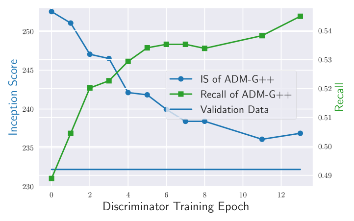
Refer to caption
(a) Discriminator epoch ablation
Refer to caption
(b) Precision/Recall trade-off
Figure 24: Ablation study of ADM-G++ on ImageNet 256x256.

Table D.1 shows experimental results of ADM in the ImageNet dataset. Cases of (a), (c), and (e) demonstrate the efficacy of the discriminator guidance. Cases of (b) and (d-1,2) are for achieving the SOTA performance with the discriminotor guidance. For (d-2), we multiply to DG weight by the norm ratio of the classifier guidance and the discriminator guidance, so to balance the guidance scale. Also, for the samples of density-ratio less than 0 in every odd denoising steps, we set wt<t0DGfragmentswfragmentstt0fragmentsDGw_{t<t_{0}}^{DG} by 0.75. Otherwise, wt<t0DG=1fragmentswfragmentstt0fragmentsDG1w_{t<t_{0}}^{DG}=1. In (e), we apply Adaptive CG/DG to report the performance of ADM-G++. As in (d-2), 1/3 of (e) experiment represents that we boost the DG weight by a factor of 3 for samples of density-ratio less than 0 in every odd denoising steps.

Figure 24-(a) shows the IS-recall curve by discriminator training epochs. We fix all the other hyperparameters except the discriminator network. Figure 24-(a) illustrates that the discriminator guidance has an effect of increasing the recall metric, which implies that a well-trained discriminator facilitates a diverse generation. Due to the diverse generation, the IS metric is decreased. Similarly, Figure 24-(b) shows that ADM-G++ significantly improves the sample diversity with a sacrifice in the precision metric.

For DiT-G++, we apply the pre-trained checkpoint from Peebles & Xie (2022) at https://github.com/facebookresearch/DiT. We draw 1,281,167 number of samples from DiT-XL/2-G to train the discriminator, with the classifier guidance scale of 1.5. In sample generation of DiT-XL/2-G++, we choose wtCG=1.25fragmentsw𝑡fragmentsCG1.25w_{t}^{CG}=1.25 for t<t0fragmentstt0t<t_{0} with t0=200fragmentst0200t_{0}=200 and wtCG=3.0fragmentsw𝑡fragmentsCG3.0w_{t}^{CG}=3.0 otherwise. We use wtDG=1fragmentsw𝑡fragmentsDG1w_{t}^{DG}=1 and do not ablate the weight scale.

D.2 Further Score Training
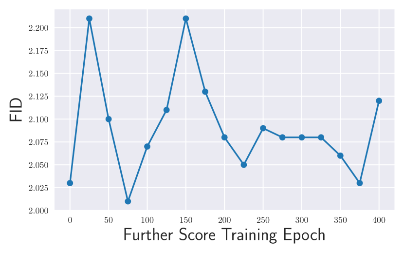
Refer to caption
Figure 25: Further score training of a pre-trained score model.

D.3 More Ablation Studies

D.3.1 Discriminator Training
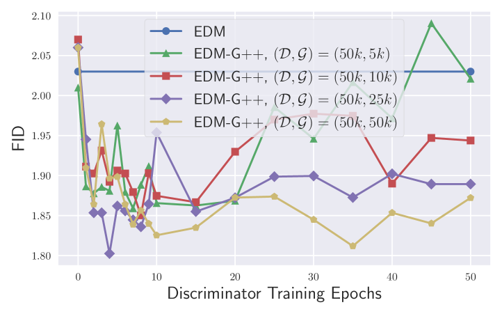
Refer to caption
(a) Full data and partial sample ablation
Refer to caption
(b) Partial data and partial sample ablation
Figure 26: Study of EDM on CIFAR-10 with respect to the number of training data. (a) is the case with full real data 𝒟𝒟\mathcal{D} and partial sample data 𝒢𝒢\mathcal{G} and (b) is the case with partial 𝒟𝒟\mathcal{D} and partial 𝒢𝒢\mathcal{G}.

Ablation of ##\# Training Data Figure 26 shows the ablation study on the number of training data on CIFAR-10. The discriminator guidance requires many samples from p𝜽fragmentspfragmentsθp_{\bm{\theta}_{\infty}} to learn the density-ratio, so this could arise the computational issue in some cases. For that, we train the discriminator with the full set of real data and a partial set of sample data in Figure 26-(a). In other words, the case of (𝒟,𝒢)=(50k,25k)fragments(D,G)(50k,25k)(\mathcal{D},\mathcal{G})=(50k,25k) represents for the case of the full use of real data as 𝒟𝒟\mathcal{D} and the half number of sample data as 𝒢𝒢\mathcal{G} in Algorithm 1. Figure 26-(b), on the other hand, uses the same number of real data for discriminator training. For both experiments, the discriminator suffers from the overffiting issue as the number of generated data decreases.

Analogous to Figure 26-(a), Figure 26-(b) shows the another ablation study on the number of training data. The situation is a bit different: in this case, we also reduce the size of real data as well as the sample data. Comparing Figure 26-(b) with Figure 26-(a), it is generally not recommendable in any cases. The overfitting arises faster, leading the performance gets worsened faster.
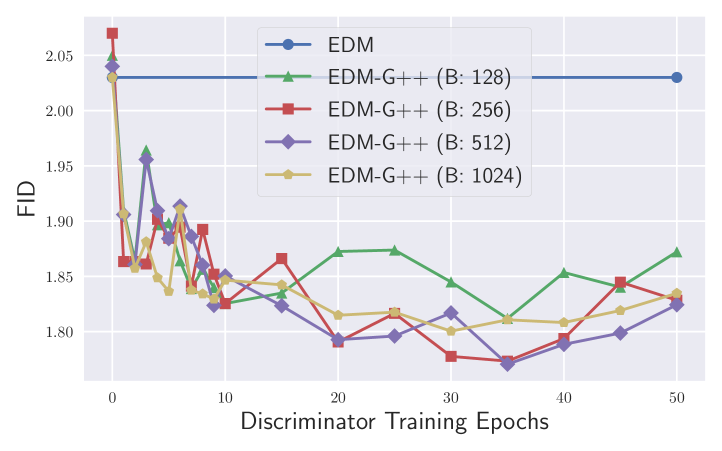
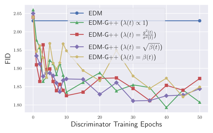
Refer to caption
(a) Batch size ablation
Refer to caption
(b) Temporal weight λ𝜆\lambda ablation
Figure 27: Study of EDM on CIFAR-10 with respect to (a) the number of training batch size and (b) the temporal weight λ𝜆\lambda.
Refer to caption
(a) Forward SDE ablation
Refer to caption
(b) Initialization ablation
Figure 28: Study of EDM on CIFAR-10 with respect to (a) the discriminator diffusing method and (b) the discriminator parameter initialization.

Ablation of ##\# Batch Size Figure 27-(a) illustrates the ablation study on the number of training batch size on CIFAR-10. Figure 27-(a) implies that the number of batch size is not a crucial factor for final performance of discriminator guidance.

Ablation of Temporal Weight λ𝜆\lambda Figure 27-(b) shows indistinguishable FID by the variance of temporal weighting function λ𝜆\lambda for ϕfragmentsLbold-italic-ϕ\mathcal{L}_{\bm{\phi}} of Eq. (4). We experiment with a uniform distribution λ(t)1fragmentsλ(t)proportional-to1\lambda(t)\propto 1, an importance-weighted (Song et al., 2021) distribution λ(t)=g2(t)σ2(t)fragmentsλ(t)fragmentsg2(t)fragmentsσ2(t)\lambda(t)=\frac{g^{2}(t)}{\sigma^{2}(t)} that is one of a common practice, and two β𝛽\beta-related distributions of λ(t)=β(t)fragmentsλ(t)fragmentsβ(t)\lambda(t)=\sqrt{\beta(t)} and λ(t)=β(t)fragmentsλ(t)β(t)\lambda(t)=\beta(t). We train the discriminator with LVP-SDE. Figure 27-(b) demonstrates that there is no significant difference between the choice of λ𝜆\lambda.

Ablation of SDE Figure 28-(a) empirically shows that using LVP-SDE as discriminator SDE performs better than using WVE-SDE. This indicates an important fact: while score training is beneficial with WVE-SDE, discriminator training best fits with LVP-SDE. We, therefore, train the discriminator with LVP-SDE as default.

Ablation of Parameter Initialization Figure 28-(b) shows that the fine-tuning performs strictly better than the training from scratch. For the setting of fine-tuning, we fix the pre-trained classifier parameters, and only train the shallow U-Net for discriminator. In contrast, we train all the parameters including that of the latent extractor, and we set fine-tuning as default in our paper.

Additionally, we find that Exponential Moving Average (EMA) has nearly no effect on the discriminator training, and we do not apply EMA of our discriminator training.

D.3.2 After Discriminator Training
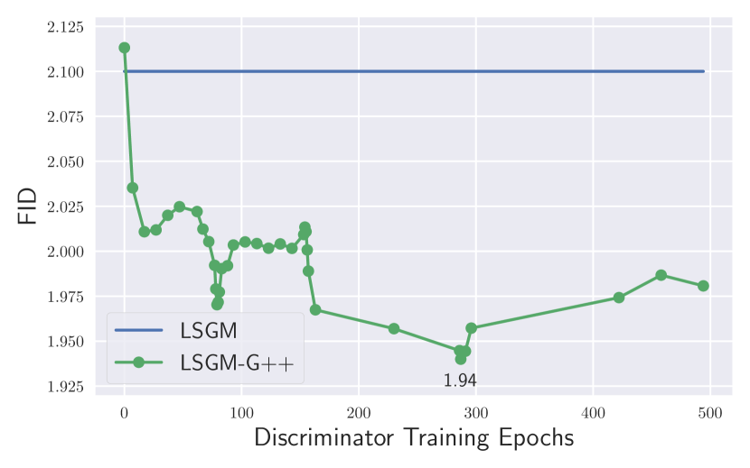
Refer to caption
Figure 29: Discriminator epoch ablation.

Ablation of Discriminator Training in Latent Diffusion on CIFAR-10 Figure 29 additionally studies LSGM on CIFAR-10. Figure 29 shows FID by discriminator training. The performance saturates after nearly 300 epochs, and it is because we do not use a pre-trained latent extractor for LSGM. Kim et al. (2022a) clarify that latent diffusion models in general have no diffusion process in the pixel space as long as models use auto-encoder structure to map data to latent. We could detour this problem by defining the diffused data as a decoded diffused latent 𝐱t=Dec(𝐳t)fragmentsx𝑡Dec(z𝑡)\mathbf{x}_{t}=Dec(\mathbf{z}_{t}), but there is no pre-trained classifier for generic diffusion strategy nor latent diffusion space. We leave it as future work in this direction. In our implementation, we train a U-Net encoder from scratch. This takes a long time to saturate, but FID improves immediately after the discriminator training.
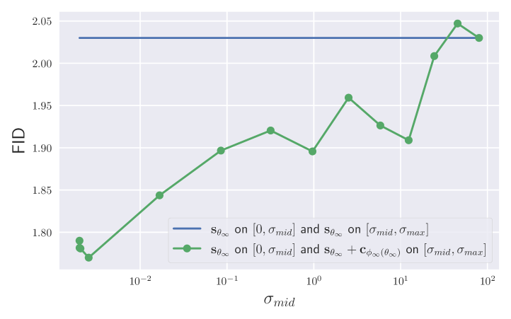
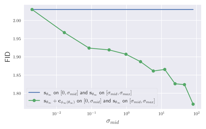
Refer to caption
(a) Minimum DG scale ablation
Refer to caption
(b) Maximum DG scale ablation
Figure 30: Study of EDM on CIFAR-10 for optimal scales to apply DG: (a) minimum scale, (b) maximum scale.

Ablation of optimal scales on CIFAR-10 Figure 30 studies the minimum/maximum diffusion scales to apply DG. For the experiment in Figure 30-(a), we divide the diffusion scales by σmidfragmentsσfragmentsmid\sigma_{mid}, and denoise with the reverse-time generative process

d𝐱t=[𝐟(𝐱t,t)g2(t)(𝐬𝜽+𝐜ϕ)(𝐱t,t)]dt¯+g(t)d𝐰¯t,fragmentsdx𝑡[f(x𝑡,t)g2(t)(sfragmentsθcfragmentsϕ)(x𝑡,t)]d¯𝑡g(t)d¯𝐰𝑡,\displaystyle\mathop{}\!\mathrm{d}\mathbf{x}_{t}=\big{[}\mathbf{f}(\mathbf{x}_{t},t)-g^{2}(t)(\mathbf{s}_{\bm{\theta}_{\infty}}+\mathbf{c}_{\bm{\phi}_{\infty}})(\mathbf{x}_{t},t)\big{]}\mathop{}\!\mathrm{d}\bar{t}+g(t)\mathop{}\!\mathrm{d}\bar{\mathbf{w}}_{t},

on the large range [σmid,σmax]fragments[σfragmentsmid,σfragmentsmax][\sigma_{mid},\sigma_{max}], and denoise with

d𝐱t=[𝐟(𝐱t,t)g2(t)𝐬𝜽(𝐱t,t)]dt¯+g(t)d𝐰¯t,fragmentsdx𝑡[f(x𝑡,t)g2(t)sfragmentsθ(x𝑡,t)]d¯𝑡g(t)d¯𝐰𝑡,\displaystyle\mathop{}\!\mathrm{d}\mathbf{x}_{t}=\big{[}\mathbf{f}(\mathbf{x}_{t},t)-g^{2}(t)\mathbf{s}_{\bm{\theta}_{\infty}}(\mathbf{x}_{t},t)\big{]}\mathop{}\!\mathrm{d}\bar{t}+g(t)\mathop{}\!\mathrm{d}\bar{\mathbf{w}}_{t},

on the small range [0,σmid]fragments[0,σfragmentsmid][0,\sigma_{mid}]. With this ablation study, we could find the optimal minimum stopping scale to apply the diffusion scale. Figure 30-(a) illustrates that the optimal stopping scale near σmid=0.0025fragmentsσfragmentsmid0.0025\sigma_{mid}^{*}=0.0025. This strictly positive optimal scale implies that either the score adjustment becomes inaccurate or the discretization error matters at the range of extremely low scale. In the density-ratio community, density-chasm problem is a well-known problem (Rhodes et al., 2020; Kato & Teshima, 2021) that depicts a poor density-ratio estimation when the two densities have distinctive supports. It arises from the training-test mismatch: the discriminator perfectly classifies real/fake, but the middle area between the real data support and the fake data support remain unoptimized. Therefore, the density-chasm problem is one of the reason for such a strictly positive optimal scale.

Figure 30-(b) studies the maximum diffusion scale to apply DG. Analogous to the experimental setting of Figure 30-(a), we divide the diffusion scales by σmidfragmentsσfragmentsmid\sigma_{mid}, and denoise with the reverse-time generative process

d𝐱t=[𝐟(𝐱t,t)g2(t)𝐬𝜽(𝐱t,t)]dt¯+g(t)d𝐰¯t,fragmentsdx𝑡[f(x𝑡,t)g2(t)sfragmentsθ(x𝑡,t)]d¯𝑡g(t)d¯𝐰𝑡,\displaystyle\mathop{}\!\mathrm{d}\mathbf{x}_{t}=\big{[}\mathbf{f}(\mathbf{x}_{t},t)-g^{2}(t)\mathbf{s}_{\bm{\theta}_{\infty}}(\mathbf{x}_{t},t)\big{]}\mathop{}\!\mathrm{d}\bar{t}+g(t)\mathop{}\!\mathrm{d}\bar{\mathbf{w}}_{t},

on the large range [σmid,σmax]fragments[σfragmentsmid,σfragmentsmax][\sigma_{mid},\sigma_{max}], and denoise with

d𝐱t=[𝐟(𝐱t,t)g2(t)(𝐬𝜽+𝐜ϕ)(𝐱t,t)]dt¯+g(t)d𝐰¯t,fragmentsdx𝑡[f(x𝑡,t)g2(t)(sfragmentsθcfragmentsϕ)(x𝑡,t)]d¯𝑡g(t)d¯𝐰𝑡,\displaystyle\mathop{}\!\mathrm{d}\mathbf{x}_{t}=\big{[}\mathbf{f}(\mathbf{x}_{t},t)-g^{2}(t)(\mathbf{s}_{\bm{\theta}_{\infty}}+\mathbf{c}_{\bm{\phi}_{\infty}})(\mathbf{x}_{t},t)\big{]}\mathop{}\!\mathrm{d}\bar{t}+g(t)\mathop{}\!\mathrm{d}\bar{\mathbf{w}}_{t},

on the small range [0,σmid]fragments[0,σfragmentsmid][0,\sigma_{mid}]. Contrastive to the minimum scale ablation study, the larger the scale DG applied, the better the performance. This means that the actual effect of DG lies in constructing the global shape of the generation, rather than denoising fine-details. In the community of diffusion models, there are only a few works that systematically divide the context generation ability and fine-detail capturing ability of diffusion models. Figure 30 clarify that DG effectively adjusts the context generation ability of diffusion models, rather than cleansing the fine-dust in images.
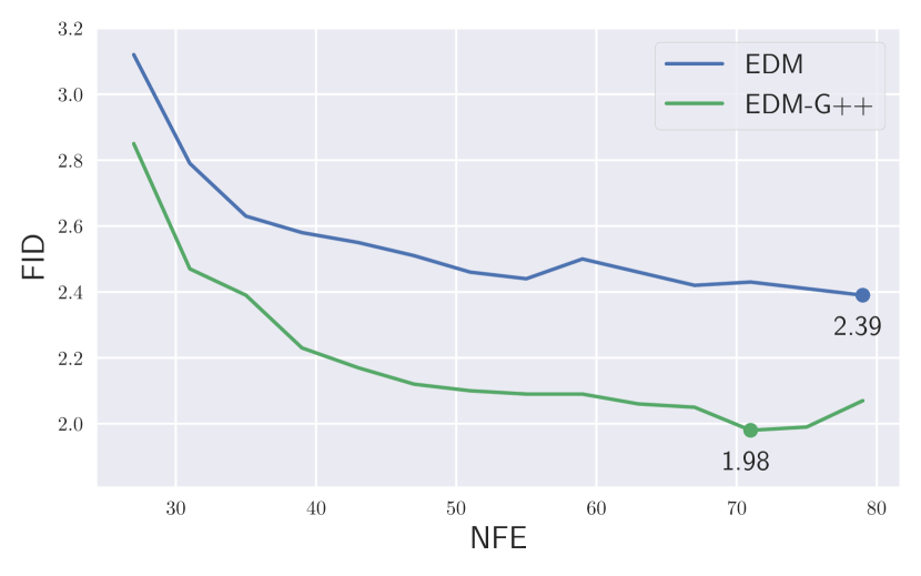
Refer to caption
Figure 31: NFE ablation on FFHQ.

Ablation of NFE on FFHQ Figure 31 illustrates FID by NFE after discriminator training. For visualization purpose, we select the best hyperparameters to experiment with, except NFE. Similar to NFE ablation on CIFAR-10, the discriminator guidance keeps enhancing FID throughout NFEs.

D.4 Uncurated Samples

Figures 32, 33, 34, 35, 36, 37, 38 compare ADM-G++ (cfg=0.10) with the vanilla ADM to illustrate how sample fidelity is improved while keeping the sample diversity. ADM-G++ (cfg=0.10) performs FID of 4.45 and recall of 0.60, and ADM performs FID of 10.94 and recall of 0.63.

Figures 39, 40, 41, 42, 43, 44, 45 compare ADM-G++ (cfg=0.75) with ADM-G (cfg=1.50). These figures show the discriminator guidance is effective in high-dimensional dataset.

Figures 46, 47, 48, 49, and 50 show uncurated samples from unconditional CIFAR-10 with LSGM-G++, unconditional CIFAR-10 with EDM-G++, conditional CIFAR-10 with EDM-G++, unconditional CelebA with Soft Truncation-G++, and unconditional FFHQ with EDM-G++.

Figure 51 shows the uncurated samples from I2I translation task.
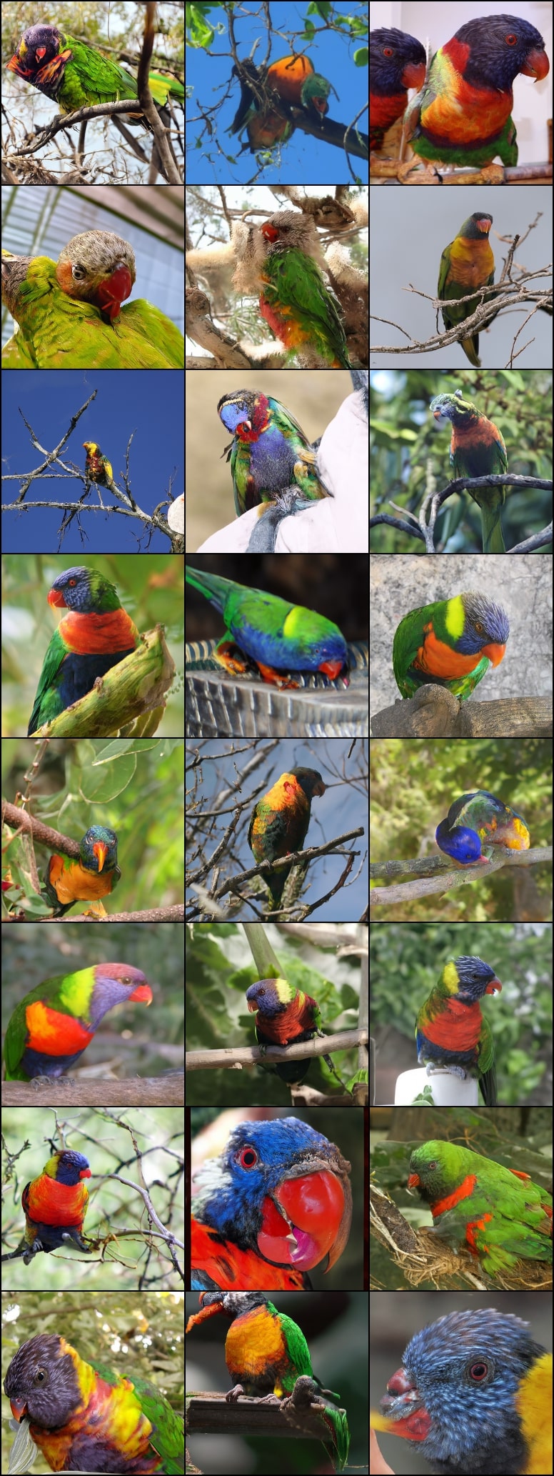
Refer to caption
(a) ADM (FID 10.94 recall 0.63)
Refer to caption
(b) ADM-G++ (FID 4.45 recall 0.60)
Figure 32: Uncurated random samples from lorikeet class (90) (a) ADM with poor FID (10.94) and good recall (0.63), (b) ADM-G++ with good FID (4.45) and good recall (0.60).
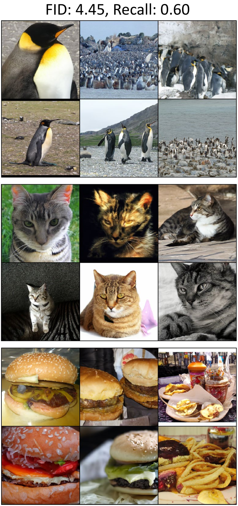
Refer to caption
(a) ADM (FID 10.94 recall 0.63)
Refer to caption
(b) ADM-G++ (FID 4.45 recall 0.60)
Figure 33: Uncurated random samples from flamingo class (130) (a) ADM with poor FID (10.94) and good recall (0.63), (b) ADM-G++ with good FID (4.45) and good recall (0.60).
Refer to caption
(a) ADM (FID 10.94 recall 0.63)
Refer to caption
(b) ADM-G++ (FID 4.45 recall 0.60)
Figure 34: Uncurated random samples from tabby cat class (281) (a) ADM with poor FID (10.94) and good recall (0.63), (b) ADM-G++ with good FID (4.45) and good recall (0.60).
Refer to caption
(a) ADM (FID 10.94 recall 0.63)
Refer to caption
(b) ADM-G++ (FID 4.45 recall 0.60)
Figure 35: Uncurated random samples from monarch butterfly class (323) (a) ADM with poor FID (10.94) and good recall (0.63), (b) ADM-G++ with good FID (4.45) and good recall (0.60).
Refer to caption
(a) ADM (FID 10.94 recall 0.63)
Refer to caption
(b) ADM-G++ (FID 4.45 recall 0.60)
Figure 36: Uncurated random samples from african elephant class (386) (a) ADM with poor FID (10.94) and good recall (0.63), (b) ADM-G++ with good FID (4.45) and good recall (0.60).
Refer to caption
(a) ADM (FID 10.94 recall 0.63)
Refer to caption
(b) ADM-G++ (FID 4.45 recall 0.60)
Figure 37: Uncurated random samples from ballon class (417) (a) ADM with poor FID (10.94) and good recall (0.63), (b) ADM-G++ with good FID (4.45) and good recall (0.60).
Refer to caption
(a) ADM (FID 10.94 recall 0.63)
Refer to caption
(b) ADM-G++ (FID 4.45 recall 0.60)
Figure 38: Uncurated random samples from fountain class (562) (a) ADM with poor FID (10.94) and good recall (0.63), (b) ADM-G++ with good FID (4.45) and good recall (0.60).
Refer to caption
(a) ADM-G (FID 4.59 recall 0.52)
Refer to caption
(b) ADM-G++ (FID 3.18 recall 0.53)
Figure 39: Uncurated random samples from lorikeet class (90) (a) ADM-G with good FID (4.59) and poor recall (0.52), (b) ADM-G++ with SOTA FID (3.18) and moderate recall (0.53).
Refer to caption
(a) ADM-G (FID 4.59 recall 0.52)
Refer to caption
(b) ADM-G++ (FID 3.18 recall 0.53)
Figure 40: Uncurated random samples from flamingo class (130) (a) ADM-G with good FID (4.59) and poor recall (0.52), (b) ADM-G++ with SOTA FID (3.18) and moderate recall (0.53).
Refer to caption
(a) ADM-G (FID 4.59 recall 0.52)
Refer to caption
(b) ADM-G++ (FID 3.18 recall 0.53)
Figure 41: Uncurated random samples from tabby cat class (281) (a) ADM-G with good FID (4.59) and poor recall (0.52), (b) ADM-G++ with SOTA FID (3.18) and moderate recall (0.53).
Refer to caption
(a) ADM-G (FID 4.59 recall 0.52)
Refer to caption
(b) ADM-G++ (FID 3.18 recall 0.53)
Figure 42: Uncurated random samples from monarch butterfly class (323) (a) ADM-G with good FID (4.59) and poor recall (0.52), (b) ADM-G++ with SOTA FID (3.18) and moderate recall (0.53).
Refer to caption
(a) ADM-G (FID 4.59 recall 0.52)
Refer to caption
(b) ADM-G++ (FID 3.18 recall 0.53)
Figure 43: Uncurated random samples from african elephant class (386) (a) ADM-G with good FID (4.59) and poor recall (0.52), (b) ADM-G++ with SOTA FID (3.18) and moderate recall (0.53).
Refer to caption
(a) ADM-G (FID 4.59 recall 0.52)
Refer to caption
(b) ADM-G++ (FID 3.18 recall 0.53)
Figure 44: Uncurated random samples from ballon class (417) (a) ADM-G with good FID (4.59) and poor recall (0.52), (b) ADM-G++ with SOTA FID (3.18) and moderate recall (0.53).
Refer to caption
(a) ADM-G (FID 4.59 recall 0.52)
Refer to caption
(b) ADM-G++ (FID 3.18 recall 0.53)
Figure 45: Uncurated random samples from fountain class (562) (a) ADM-G with good FID (4.59) and poor recall (0.52), (b) ADM-G++ with SOTA FID (3.18) and moderate recall (0.53).
Refer to caption
Figure 46: Uncurated random samples from LSGM-G++ on unconditional CIFAR10 (FID: 1.94).
Refer to caption
Figure 47: Uncurated random samples from EDM-G++ on unconditional CIFAR10 (FID: 1.77).
Refer to caption
Figure 48: Uncurated random samples from EDM-G++ on conditional CIFAR10 (FID: 1.64).
Refer to caption
Figure 49: Uncurated random samples from Soft Truncation-G++ on unconditional CelebA (FID: 1.34).
Refer to caption
Figure 50: Uncurated random samples from EDM-G++ on unconditional FFHQ (FID: 1.98).
Refer to caption
(a) Cat (Source)
Refer to caption
(b) SDEdit (FID: 74.02)
Refer to caption
(c) SDEdit + DG (FID: 61.92)
Figure 51: Uncurated random translated samples from (a) source cat, (b) SDEdit (FID: 74.02, L2: 49.22, PSNR: 19.21, SSIM: 0.42), and (c) SDEdit + DG with wtDG=8fragmentsw𝑡fragmentsDG8w_{t}^{DG}=8 (FID: 61.92, L2: 50.62, PSNR: 18.94, SSIM: 0.41).
Conversion to HTML had a Fatal error and exited abruptly. This document may be truncated or damaged.