Self-Supervised Continual Graph Learning in Adaptive Riemannian Spaces

Abstract

Continual graph learning routinely finds its role in a variety of real-world applications where the graph data with different tasks come sequentially. Despite the success of prior works, it still faces great challenges. On the one hand, existing methods work with the zero-curvature Euclidean space, and largely ignore the fact that curvature varies over the coming graph sequence. On the other hand, continual learners in the literature rely on abundant labels, but labeling graph in practice is particularly hard especially for the continuously emerging graphs on-the-fly. To address the aforementioned challenges, we propose to explore a challenging yet practical problem, the self-supervised continual graph learning in adaptive Riemannian spaces. In this paper, we propose a novel self-supervised Riemannian Graph Continual Learner (RieGrace). In RieGrace, we first design an Adaptive Riemannian GCN (AdaRGCN), a unified GCN coupled with a neural curvature adapter, so that Riemannian space is shaped by the learnt curvature adaptive to each graph. Then, we present a Label-free Lorentz Distillation approach, in which we create teacher-student AdaRGCN for the graph sequence. The student successively performs intra-distillation from itself and inter-distillation from the teacher so as to consolidate knowledge without catastrophic forgetting. In particular, we propose a theoretically grounded Generalized Lorentz Projection for the contrastive distillation in Riemannian space. Extensive experiments on the benchmark datasets show the superiority of RieGrace, and additionally, we investigate on how curvature changes over the graph sequence.

Introduction

Continual graph learning is emerging as a hot research topic which successively learns from a graph sequence with different tasks (Febrinanto et al. 2022). In general, it aims at gradually learning new knowledge without catastrophic forgetting the old ones across sequentially coming tasks. Centered around fighting with forgetting, a series of methods (Kim, Yun, and Kang 2022; Galke et al. 2021) have been proposed recently. Despite the success of prior works, continual graph learning still faces tremendous challenges.

Challenge 1: An adaptive Riemannian representation space. To the best of our knowledge, existing methods work with Euclidean space, the zero-curvature Riemannian space (Zhang, Song, and Tao 2022; Zhou and Cao 2021; Wang et al. 2020). However, in continual graph learning, the curvature of a graph remains unknown until its arrival. In particular, the negatively curved Riemannian space, hyperbolic space, is well-suited for graphs presenting hierarchical patterns or tree-like structures (Krioukov et al. 2010; Nickel and Kiela 2017). The underlying geometry shifts to be positively curved, hyperspherical space, when cyclical patterns (e.g., triangles or cliques) become dominant (Bachmann, Bécigneul, and Ganea 2020). Even more challenging, the curvature usually varies over the coming graph sequence as shown in the case study. Thus, it calls for a smart graph encoder in the Riemannian space with adaptive curvature for each coming graph successively.

Challenge 2: Continual graph learning without supervision. Existing continual graph learners (Cai et al. 2022; Wang et al. 2022) are trained in the supervised fashion, and thereby rely on abundant labels for each learning task. Labeling graphs requires either manual annotation or paying for permission in practice. It is particularly hard and even impossible when graphs are continuously emerging on-the-fly. In this case, self-supervised learning is indeed appealing, so that we can acquire knowledge from the unlabeled data themselves. Though self-supervised learning on graphs is being extensively studied (Veličković et al. 2019; Qiu et al. 2020; Yin et al. 2022), existing methods are trained offline. That is, they are not applicable for continual graph learning, and naive application results in catastrophic forgetting in the successive learning process (Lange et al. 2022; Ke et al. 2021). Unfortunately, self-supervised continual graph learning is surprisingly under-investigated in the literature.

Consequently, it is vital to explore how to learn and memorize knowledge free of labels for continual graph learning in adaptive Riemannian spaces. Thus, we propose the challenging yet practical problem of self-supervised continual graph learning in adaptive Riemannian spaces.

In this paper, we propose a novel self-supervised Riemannian Graph Continual Learner (RieGrace). To address the first challenge, we design an Adaptive Riemannian GCN (AdaRGCN), which is able to shift among any hyperbolic or hyperspherical space adaptive to each graph. In AdaRGCN, we formulate a unified Riemannian graph convolutional network (RGCN) of arbitrary curvature, and design a CurvNet inspired by Forman-Ricci curvature in Riemannian geometry. CurvNet is a neural module in charge of curvature adaptation, so that we induce a Riemannian space shaped by the curvature learnt from the task graph. To address the second challenge, we propose a novel label-free Lorentz distillation approach to consolidate knowledge without catastrophic forgetting. Specifically, we create teacher-student AdaRGCN for the graph sequence. When receiving a new graph, the student is created from the teacher. The student distills from the intermedian layer of itself to acquire knowledge of current graph (intra-distillation), and in the meanwhile, distills from the teacher to preserve the past knowledge (inter-distillation). In our approach, we propose to consolidate knowledge via contrastive distillation, but it is particularly challenging to contrast between different Riemannian spaces. To bridge this gap, we formulate a novel Generalized Lorentz Projection (GLP). We prove GLP is closed on Riemannian spaces, and show its relationship to the well-known Lorentz transformation.

In short, noteworthy contributions are summarized below:

• Problem. We propose the problem of self-supervised continual graph learning in adaptive Riemannian spaces, which is the first attempt, to the best of our knowledge, to study continual graph learning in non-Euclidean space.

• Methodology. We present a novel RieGrace, where we design a unified RGCN with CurvNet to shift curvature among hyperbolic or hyperspherical spaces adaptive to each graph, and propose the Label-free Lorentz Distillation with GLP for self-supervised continual learning.

• Experiments. Extensive experiments on the benchmark datasets show that RieGrace even outperforms the state-of-the-arts supervised methods, and the case study gives further insight on the curvature over the graph sequence with the notion of embedding distortion.

Preliminaries

In this section, we first introduce the fundamentals of Riemannian geometry necessary to understand this work, and then formulate the studied problem, self-supervised continual graph learning in general Riemannian space. In short, we are interested in how to learn an encoder $\mathbf{\Phi}$ that is able to sequentially learn on coming graphs $G_{1},\dots,G_{T}$ in adaptive Riemannian spaces without external supervision.

Riemannian Geometry

Riemannian Manifold.

A Riemannian manifold $(\mathcal{M},g)$ is a smooth manifold $\mathcal{M}$ equipped with a Riemannian metric $g$. Each point $\mathbf{x}$ on the manifold is associated with a tangent space $\mathcal{T}_{\mathbf{x}}\mathcal{M}$ that looks like Euclidean. The Riemannian metric $g$ is the collection of inner products at each point $\mathbf{x}\in\mathcal{M}$ regarding its tangent space. For $\mathbf{x}\in\mathcal{M}$, the exponential map at $\mathbf{x}$, $exp_{\mathbf{x}}(\mathbf{v}):\mathcal{T}_{\mathbf{x}}\mathcal{M}\to\mathcal{M}$, projects the vector of the tangent space at $\mathbf{x}$ onto the manifold, and the logarithmic map $log_{\mathbf{x}}(\mathbf{y}):\mathcal{M}\to\mathcal{T}_{\mathbf{x}}\mathcal{M}$ is the inverse operator.

Curvature.

In Riemannian geometry, the curvature is the notion to measure how a smooth manifold deviates from being flat. If the curvature is uniformly distributed, the manifold $\mathcal{M}$ is called the space of constant curvature $\kappa$. In particular, the space is hyperspherical $\mathbb{S}$ with $\kappa>0$ when it is positively curved, and hyperbolic $\mathbb{H}$ with $\kappa<0$ when negatively curved. Euclidean space is flat space with $\kappa=0$, and can be considered as a special case in Riemannian geometry.

Problem Formulation

In the continual graph learning, we will receive a sequence of disjoint tasks $\mathcal{T}=\{\mathcal{T}_{1},\dots,\mathcal{T}_{t},\dots,\mathcal{T}_{T}\}$, and each task is defined on a graph $G=\{\mathcal{V},\mathcal{E}\}$, where $\mathcal{V}=\{v_{1},\cdots,v_{N}\}$ is the node set, and $\mathcal{E}=\{(v_{i},v_{j})\}\subset\mathcal{V}\times\mathcal{V}$ is the edge set. Each node $v_{i}$ is associated with node feature $\mathbf{x}_{i}$ and a category $y_{i}\in\mathcal{Y}_{k}$, where $\mathcal{Y}_{k}$ is the label set of $k$ categories.

Definition 1 (Graph Sequence).

The sequence of tasks in graph continual learning is described as a graph sequence $\mathcal{G}=\{G_{1},\dots,G_{T}\}$, and each graph $G_{t}$ corresponds to a task $\mathcal{T}_{t}$. Each task contains a training node set $\mathcal{V}_{t}^{tr}$ and a testing node set $\mathcal{V}_{t}^{te}$ with node features $X_{t}^{tr}$ and $X_{t}^{te}$.

In this paper, we study the task-incremental learning in adaptive Riemannian space whose curvature is able to successively match each task graph. When a new graph arrives, the learnt parameters are memorized but historical graphs are dropped, and additionally, no labels are provided in the learning process. We give the formal definition as follows:

Definition 2 (Self-Supervised Continual Graph Learning in Adaptive Riemannian Space).

Given a graph sequence $\mathcal{G}$ with tasks $\mathcal{T}$, we aim at learning an encoder $\mathbf{\Phi}:v\to\mathbf{h}\in\mathcal{M}^{d,k}$ in absence of labels in adaptive Riemannian space, so that the encoder is able to continuously consolidate the knowledge for current task without catastrophically forgetting the knowledge for previous ones.

Essentially different from the continual graph learners of prior works, we study with a more challenging yet practical setting: i) rather than Euclidean space, the encoder $\mathbf{\Phi}$ works with an adaptive Riemannian space suitable for each task, and ii) is able to learn and memorize knowledge without labels for continuously emerging graphs on-the-fly.

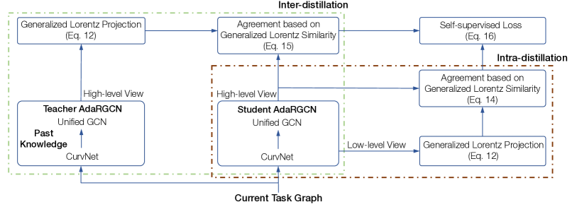
Figure 1: Overall architecture of RieGrace. We design the AdaRGCN which successively adapts its curvature for current task graph with CurvNet, and propose Label-free Lorentz Distillation for continual graph learning. In each learning session, i) the student is created from the teacher with the same architecture, ii) jointly performs intra-distillation from itself and inter-distillation from the teacher with GLP to consolidate knowledge, and iii) becomes the teacher for the next learning session.

Methodology

To address this problem, we propose a novel Self-supervised Riemannian Graph Continual Learner (RieGrace) We illustrate the overall architecture of RieGrace in Figure 1. In the nutshell, we first design a unified graph convolutional network (AdaRGCN) on the Riemannian manifold shaped by the learnt curvature adaptive to each coming graph. Then, we propose a label-free Lorentz distillation approach to consolidate knowledge without catastrophic forgetting.

Representation Space.

First of all, we introduce the Riemannian manifolds we use in this paper before we construct RieGrace on them. We opt for the hyperboloid (Lorentz) model for hyperbolic space and the corresponding hypersphere model for hyperspherical space with the unified formalism, owing to the numerical stability and closed form expressions (Liu, Nickel, and Kiela 2019).

Formally, we have a $d$-dimensional manifold of curvature $\kappa$, $\mathcal{M}^{d,\kappa}=\{\mathbf{x}\in\mathbb{R}^{d+1}|\ \langle\mathbf{x},\mathbf{x}\rangle_{\kappa}=\frac{1}{\kappa}\}$ with $\kappa\neq 0$, whose origin is denoted as $\mathcal{O}=(|\kappa|^{-\frac{1}{2}},0,\cdots,0)\in\mathcal{M}^{d,\kappa}$. The curvature-aware inner product $\langle\cdot,\cdot\rangle_{\kappa}$ is defined as

$$\langle\mathbf{x},\mathbf{y}\rangle_{\kappa}=\mathbf{x}^{\top}\operatorname{diag}(sign(\kappa),1,\cdots,1)\mathbf{y},\vspace{-0.07in}$$ (1)

and thus the tangent space at $\mathbf{x}$ is given as $\mathcal{T}_{\mathbf{x}}\mathcal{M}^{d,\kappa}=\{\mathbf{v}\in\mathbb{R}^{d+1}|\ \langle\mathbf{v},\mathbf{x}\rangle_{\kappa}=0\}$. In particular, for the positive curvature, $\mathcal{M}^{d,\kappa}$ is the hypersphere model $\mathbb{S}^{d,\kappa}$ and $\langle\cdot,\cdot\rangle_{\kappa}$ is the the standard inner product on $\mathbb{R}^{d+1}$. For the negative curvature, $\mathcal{M}^{d,\kappa}$ is the hyperboloid model $\mathbb{H}^{d,\kappa}$ and $\langle\cdot,\cdot\rangle_{\kappa}$ is the Minkowski inner product. The operators with the unified formalism on $\mathcal{M}^{d,\kappa}$ is summarized in Table 1, where $v=\sqrt{|\kappa|}\|\mathbf{v}\|_{\kappa}$, $\beta=\kappa\langle\mathbf{x},\mathbf{y}\rangle_{\kappa}$ and $\|\mathbf{v}\|_{\kappa}^{2}=\langle\mathbf{v},\mathbf{v}\rangle_{\kappa}$ for $\mathbf{v}\in\mathcal{T}_{\mathbf{x}}\mathcal{M}^{d,\kappa}$. We utilize the curvature-aware trigonometric function the same as Skopek, Ganea, and Bécigneul (2020).

Operator	Unified formalism in $\mathcal{M}^{d,\kappa}$
Distance Metric	$d_{\mathcal{M}}(\mathbf{x},\mathbf{y})=\frac{1}{\sqrt{|\kappa|}}\cos^{-1}_{\kappa}\left(\kappa\langle\mathbf{x},\mathbf{y}\rangle_{\kappa}\right)$
Exponential Map	$exp_{\mathbf{x}}^{\kappa}(\mathbf{v})=\cos_{\kappa}\left(\alpha\right)\mathbf{x}+\frac{\sin_{\kappa}\left(\alpha\right)}{\alpha}\mathbf{v}$
Logarithmic Map	$log_{\mathbf{x}}^{\kappa}(\mathbf{y})=\frac{\cos^{-1}_{\kappa}\left(\beta\right)}{\sin_{\kappa}\left(\cos^{-1}_{\kappa}\left(\beta\right)\right)}\left(\mathbf{y}-\beta\mathbf{x}\right)$
Scalar Multiply	$r\otimes_{\kappa}\mathbf{x}=exp_{\mathcal{O}}^{\kappa}\left(r\ log_{\mathcal{O}}^{\kappa}(\mathbf{x})\right)$

Table 1: Curvature-aware operations in manifold $\mathcal{M}^{d,\kappa}$.

Adaptive Riemannian GCN

Recall that the curvature of task graph remains unknown until its arrival. We propose an adaptive Riemannian GCN (AdaRGCN), a unified GCN of arbitrary curvature coupled with a CurvNet, a neural module for curvature adaptation. AdaRGCN shifts among hyperbolic and hyperspherical spaces accordingly to match the geometric pattern of each graph, essentially distinguishing itself from prior works.

Unified GCN of Arbitrary Curvature.

Recent studies in Riemannian graph learning mainly focus on the design of GCNs in manifold $\mathcal{M}^{d,\kappa}$ with negative curvatures (hyperboloid model), but the unified GCN of arbitrary curvature has rarely been touched yet. To bridge this gap, we propose a unified GCN of arbitrary curvature, generalizing from the zero-curvature GAT (Veličković et al. 2018). Specifically, we introduce the operators with unified formalism on $\mathcal{M}^{d,\kappa}$.

Feature transformation is a basic operation in neural network. For $\mathbf{h}\in\mathcal{M}^{d,\kappa}$, we perform the transformation via the $\kappa$-left-multiplication $\boxtimes_{\kappa}$ defined by $exp_{\mathcal{O}}^{\kappa}(\cdot)$ and $log_{\mathcal{O}}^{\kappa}(\cdot)$,

$$\mathbf{W}\boxtimes_{\kappa}\mathbf{h}=exp_{\mathcal{O}}^{\kappa}\left(\left[\ 0\ \|\ \mathbf{W}\ log_{\mathcal{O}}^{\kappa}(\mathbf{h})_{[1:d]}\right]\right),\vspace{-0.05in}$$ (2)

where $\mathbf{W}\in\mathbb{R}^{d^{\prime}\times d}$ is weight matrix, and $[\cdot\|\cdot]$ denotes concatenation. Note that, $[log_{\mathcal{O}}^{\kappa}(\mathbf{h})]_{0}=0$ holds, $\forall\mathbf{h}\in\mathcal{M}^{d,\kappa}$.

The advantage of Eq. (2) is that logarithmically mapped vector lies in the tangent space $\mathcal{T}_{\mathcal{O}}\mathcal{M}^{d,\kappa}$ for any $\mathbf{W}$ so that we can utilize $exp_{\mathcal{O}}^{\kappa}(\cdot)$ safely, which is not guaranteed in direct combination formalism of $exp_{\mathcal{O}}^{\kappa}(\mathbf{W}log_{\mathcal{O}}^{\kappa}(\mathbf{h}))$. Similarly, we give the formulation of applying function $f(\cdot)$,

$$f_{\kappa}(\mathbf{h})=exp_{\mathcal{O}}^{\kappa}\left(\left[\ 0\ \|\ f(log_{\mathcal{O}}^{\kappa}(\mathbf{h}))_{[1:d]}\right]\right).\vspace{-0.035in}$$ (3)

Neighborhood aggregation is a weighted arithmetic mean and also the geometric centroid of the neighborhood features essentially (Wu et al. 2019). Fréchet mean follows this meaning in Riemannian space, but unfortunately does not have a closed form solution (Law et al. 2019). Alternatively, we define neighborhood aggregation as the geometric centroid of squared distance, in spirit of Fréchet mean, to enjoy both mathematical meaning and efficiency. Given a set of neighborhood features $\mathbf{h}_{j}\in\mathcal{M}^{d,\kappa}$ centered around $v_{i}$, the closed form aggregation is derived as follows:

where $\bar{\mathcal{N}}_{i}$ is the neighborhood of $v_{i}$ including itself, and $\nu_{ij}$ is the attention weight.

Different from Law et al. (2019); Zhang et al. (2021), we generalize the centroid from hyperbolic space to the Riemannian space of arbitrary curvature $\mathcal{M}^{d,\kappa}$, and show its connection to gyromidpoint of $\kappa$-sterographical model theoretically. Now, we prove that arithmetic mean in Eq. (4) is the closed form expression of the geometric centroid.

Proposition 1.

Given a set of points $\mathbf{h}_{j}\in\mathcal{M}^{d,\kappa}$ each attached with a weight $\nu_{ij}$, $j\in\Omega$, the centroid of squared distance $\mathbf{c}$ in the manifold is given as minimization problem:

$$\min_{\mathbf{c}\in\mathcal{M}^{d,\kappa}}\ \ \sum\nolimits_{j\in\Omega}\nu_{ij}d_{\mathcal{M}}^{\ 2}\left(\mathbf{h}_{j},\mathbf{c}\right),\vspace{-0.07in}$$ (5)

Eq. (4) is the closed form solution, $\mathbf{c}=AGG_{\kappa}(\{\mathbf{h}_{j},\nu_{ij}\}_{i})$.

Proof.

We have $\mathbf{c}=\arg\min_{\mathbf{c}\in\mathcal{M}^{d,\kappa}}\sum_{j\in\Omega}\nu_{ij}d_{\kappa}^{\ 2}\left(\mathbf{h}_{j},\mathbf{c}\right)$, and $\mathbf{c}$ is in the manifold $\mathbf{c}\in\mathcal{M}^{d,\kappa}$, i.e., $\langle\mathbf{c},\mathbf{c}\rangle_{\kappa}=\frac{1}{\kappa}$. Please refer to the Appendix for the details. ∎

Attention mechanism is equipped for neighborhood aggregation as the importance of neighbor nodes are usually different. We study the importance between a neighbor $v_{j}$ and center node $v_{i}$ by an attention function in tangent space,

$$ATT_{\kappa}(\mathbf{x}_{i},\mathbf{x}_{j},\mathbf{\theta})=\bm{\theta}^{\top}\left[log_{\mathcal{O}}^{\kappa}(\mathbf{x}_{i})||log_{\mathcal{O}}^{\kappa}(\mathbf{x}_{j})\right],$$ (6)

parameterized by $\bm{\theta}$, and then attention weight is given by $\nu_{ij}=Softmax_{j\in\mathcal{N}_{i}}(ATT_{\kappa}(\mathbf{x}_{i},\mathbf{x}_{j},\bm{\theta}))$.

We formulate the convolutional layer on $\mathcal{M}^{d,\kappa}$ with proposed operators. The message passing in the $l^{th}$ layer is

$$\mathbf{h}_{i}^{(l)}=\delta_{\kappa}\left(AGG_{\kappa}(\{\mathbf{x}_{j},\nu_{ij}\}_{i})\right),\mathbf{x}_{i}=\mathbf{W}\boxtimes_{\kappa}\mathbf{h}_{i}^{(l-1)},\vspace{-0.05in}$$ (7)

where $\delta_{\kappa}(\cdot)$ is the nonlinearity. Consequently, we build the unified GCN by stacking multiple convolutional layers, and its curvature is adaptively learnt for each task graph with a novel neural module designed as follows.

Curvature Adaptation.

We aim to learn the curvature of any graph with a function $f:G\to\kappa$, so that the Riemannian space is able to successively match the geometric pattern of the task graph. To this end, we design a simple yet effective network, named CurvNet, based on the notion of Forman-Ricci curvature in Riemannian geometry.

Theory on Graph Curvature: Forman-Ricci curvature defines the curvature for an edge $(v_{i},v_{j})$, and Weber, Saucan, and Jost (2017) give the reformulation on the neighborhoods of its two end nodes,

where $w_{i}$ and $\gamma_{ij}$ are the weights associated with nodes and edges, respectively. $w_{i}$ is defined by the degree information of the nodes connecting to $v_{i}$, and $\gamma_{ij}=\frac{w_{i}}{\sqrt{w_{i}^{2}+w_{j}^{2}}}$. According to (Cruceru, Bécigneul, and Ganea 2021), $v_{i}$’s curvature is then given by averaging $F_{ij}$ over its neighborhood. In other words, the curvature of a node is induced by the node weights over its 2-hop neighborhood.

We propose CurvNet, a 2-layer graph convolutional net, to approximate the map from node weights to node curvatures. CurvNet aggregates and transforms the information over 2-hop neighborhood by stacking convolutional layer,

$$\mathbf{Z}^{(l)}=\operatorname{GCN}(\mathbf{Z}^{(l-1)},\mathbf{M}^{(l)}),\vspace{-0.07in}$$ (9)

twice, where $\mathbf{M}^{(l)}$ is the $l^{th}$ layer parameters. CurvNet can be built with any GCN, and we utilize Kipf and Welling (2017) in practice. The input features are node weights defined by degree information, $\mathbf{Z}^{(0)}=\mathbf{A}\operatorname{diag}(d_{1},\cdots,d_{N})$. $\mathbf{A}$ is the adjacency matrix, and $d_{i}$ is the degree of $v_{i}$. The graph curvature $\kappa$ is given as the mean of node curvatures (Cruceru, Bécigneul, and Ganea 2021), and accordingly, we readout the graph curvature by $\kappa=MeanPooling(\mathbf{Z}^{(2)})$.

Label-free Lorentz Distillation

To consolidate knowledge free of labels, we propose the Label-free Lorentz Distillation approach for continual graph learning, in which we create teacher-student AdaRGCN as shown in Figure 1. In each learning session, the student acquires knowledge for current task graph $G_{t}$ by distilling from itself, intra-distillation, and preserves past knowledge by distilling from the teacher, inter-distillation. The student finished intra- and inter-distillation becomes the teacher when new task $G_{(t+1)}$ arrives, so that we successively consolidate knowledge in the graph sequence without catastrophic forgetting.

Input: Current tack $G_{t}$, Parameters learnt from previous tasks $G_{1},\cdots,G_{t-1}$

Output: Parameters of AdaRGCN

1 while not converging do

       // Teacher-Student AdaRGCN

2       Froze the parameters of the teacher network;

3       $\mathbf{X}^{t,H}\leftarrow\text{AdaRGCN}_{teacher}$;

4       $\{\mathbf{X}^{s,H},\mathbf{X}^{s,L}\}\leftarrow\text{AdaRGCN}_{student}$;

       // Label-Free Distillation(GLP)

5       for each node $v_{i}$ in $G_{t}$ do

6             Intra-distillation: Learn for current task by contrasting with Eq. (14);

7             Inter-distillation: Learn from the teacher by contrasting with Eq. (15);

8            

9       end for

      // Update Student Parameters

10       Compute gradients of the overall objective:

$$\nabla_{\mathbf{\Theta}_{student},\{\mathbf{W},\mathbf{b}\}}\ \ \mathcal{J}_{intra}+\lambda\mathcal{J}_{inter}.$$

11 end while

Algorithm 1 RieGrace. Self-Supervised Continual Graph Learning in Adaptive Riemannian Spaces

In our approach, we propose to distill knowledge via contrastive loss in Riemannian space. Though knowledge distillation has been applied to video and text (Guo et al. 2023) and similar idea on graphs has been proposed in Euclidean space (Yu et al. 2022; Tian, Krishnan, and Isola 2020), they CANNOT be applied to Riemannian space owing to essential distinction in geometry. Specifically, it lacks a method to contrast between Riemannian spaces with either different dimension or different curvature for the distillation. To bridge this gap, we propose a novel formulation, Generalized Lorentz Projection.

Generalized Lorentz Projection (GLP) & Lorentz Layer.

We aim to contrast between $\mathbf{x}\in\mathcal{M}^{d_{1},\kappa_{1}}$ and $\mathbf{y}\in\mathcal{M}^{d_{2},\kappa_{2}}$. The obstacle is that both dimension and curvature are incomparable ($d_{1}\neq d_{2}$, $\kappa_{1}\neq\kappa_{2}$). A naive way is to use logarithmic and exponential maps with a tangent space. However, these maps are range to infinity, and trend to suffer from stability issue (Chen et al. 2022). Such shortcomings weaken its ability for the distillation, as shown in the experiment.

Fortunately, Lorentz transformation in the Einstein’s special theory of relativity performs directly mapping between Riemannian spaces, which can be decomposed into a combination of Lorentz boost $\mathbf{B}$ and rotation $\mathbf{R}$ (Dragon 2012). Formally, for $\mathbf{x}\in\mathcal{M}^{d,\kappa}$, $\mathbf{B}\mathbf{x}\in\mathcal{M}^{d,\kappa}$ and $\mathbf{R}\mathbf{x}\in\mathcal{M}^{d,\kappa}$ given blocked $\mathbf{B},\mathbf{R}\in\mathbb{R}^{(d+1)\times(d+1)}$ with positive semi-definiteness and special orthogonality, respectively. Though the clean formalism is appealing, it fails to tackle our challenge: i) The constraints on definiteness or orthogonality render the optimization problematic. ii) Both dimension and curvature are fixed, i.e., they cannot be changed over time. Recently, Chen et al. (2022) make effort to support different dimensions, but still restricted in the same curvature. Indeed, it is difficult to assure closeness of the operation especially when curvatures (i.e., shape of the manifold) are different.

In this work, we propose a novel Generalized Lorentz Projection (GLP) in spirit of Lorentz transformation so as to map between Riemannian spaces with different dimensions or curvatures. To avoid the constrained optimization, we reformalize GLP to learn a transformation matrix $\mathbf{W}\in\mathbb{R}^{d_{2}\times d_{1}}$. The relational behind is that $\mathbf{W}$ linearly transforms both dimension and curvature with a carefully designed formulation based on a Lorentz-type multiplication. Formally, given $\mathbf{x}\in\mathcal{M}^{d_{1},\kappa_{1}}$ and the target manifold $\mathcal{M}^{d_{2},\kappa_{2}}$ to map onto, $GLP^{d_{1},\kappa_{1}\to d_{2},\kappa_{2}}_{\mathbf{x}}(\cdot)$ at $\mathbf{x}$ is defined as follows,

$$GLP^{d_{1},\kappa_{1}\to d_{2},\kappa_{2}}_{\mathbf{x}}\left(\left[\begin{array}[]{cc}w&\mathbf{0}^{\top}\\ \mathbf{0}&\mathbf{W}\end{array}\right]\right)=\left[\begin{array}[]{cc}w_{0}&\mathbf{0}^{\top}\\ \mathbf{0}&\mathbf{W}\end{array}\right],\vspace{-0.03in}$$ (10)

so that we have

$$GLP^{d_{1},\kappa_{1}\to d_{2},\kappa_{2}}_{\mathbf{x}}\left(\left[\begin{array}[]{cc}w&\mathbf{0}^{\top}\\ \mathbf{0}&\mathbf{W}\end{array}\right]\right)\left[\begin{array}[]{c}x_{0}\\ \mathbf{x}_{s}\end{array}\right]=\left[\begin{array}[]{c}w_{0}x_{0}\\ \mathbf{W}\mathbf{x}_{s}\end{array}\right],\vspace{-0.03in}$$ (11)

where $w\in\mathbb{R}$, $w_{0}=\sqrt{\frac{|\kappa_{1}|}{|\kappa_{2}|}\cdot\frac{1-\kappa_{2}\ell(\mathbf{W},\mathbf{x}_{s})}{1-\kappa_{1}\langle\mathbf{x}_{s},\mathbf{x}_{s}\rangle}}$, and $\ell(\mathbf{W},\mathbf{x}_{s})=\left\|\mathbf{W}\mathbf{x}_{s}\right\|^{2}$. (The derivation is given in Appendix.)

Next, we study theoretical aspects of the proposed GLP. First and foremost, we prove that GLP is closed in Riemannian spaces with different dimensions or curvatures, so that the mapping is done correctly.

Proposition 2.

$GLP^{d_{1},\kappa_{1}\to d_{2},\kappa_{2}}_{\mathbf{x}}\left(\bar{\mathbf{W}}\right)\mathbf{x}\in\mathcal{M}^{d_{2},\kappa_{2}}$ holds, $\forall\mathbf{x}\in\mathcal{M}^{d_{1},\kappa_{1}}$, where $\bar{\mathbf{W}}=\operatorname{diag}([w,\mathbf{W}])$.

Proof.

$\mathbf{L}=GLP^{d_{1},\kappa_{1}\to d_{2},\kappa_{2}}_{\mathbf{x}}(\bar{\mathbf{W}})$, and $\langle\mathbf{L}\mathbf{x},\mathbf{L}\mathbf{x}\rangle_{\kappa_{2}}=\frac{1}{\kappa_{2}}$ holds. Please refer to Appendix for the details. ∎

Second, we prove that GLP matrices cover all valid Lorentz rotation. That is, the proposed GLP can be considered as a generalization of Lorentz rotation.

Proposition 3.

The set of GLP matrices projecting within $\mathcal{M}^{d_{1},\kappa_{1}}$ is $\mathcal{W}_{\mathbf{x}}=\{\text{GLP}^{d_{1},\kappa_{1}\to d_{1},\kappa_{1}}_{\mathbf{x}}(\mathbf{W})\}$. Lorentz rotation set is $\mathcal{Q}=\{\mathbf{R}\}$. $\mathcal{Q}\subseteq\mathcal{W}_{\mathbf{x}}$ holds, $\forall\mathbf{x}\in\mathcal{M}^{d_{1},\kappa_{1}}$.

Proof.

$\forall\mathbf{R}$, $GLP^{d_{1},\kappa_{1}\to d_{1},\kappa_{1}}_{\mathbf{x}}(\mathbf{R})=\mathbf{R}$ holds, analog to Parseval’s theorem. Please refer to Appendix for the details and further theoretical analysis. ∎

Now, we are ready to score the similarity between $\mathbf{x}\in\mathcal{M}^{d_{1},\kappa_{1}}$ and $\mathbf{y}\in\mathcal{M}^{d_{2},\kappa_{2}}$. Specifically, we add the bias for GLP, and formulate a Lorentz Layer (LL) as follows:

where $\mathbf{W}\in\mathbb{R}^{d_{2}\times d_{1}}$ and $\mathbf{b}\in\mathbb{R}^{d_{2}}$ denote the weight and bias, respectively. $\ell(\mathbf{W},\mathbf{x}_{s})=\left\|\mathbf{W}\mathbf{x}_{s}+\mathbf{b}\right\|^{2}$ for $w_{0}$. It is easy to verify $LL^{d_{1},\kappa_{1}\to d_{2},\kappa_{2}}_{\mathbf{x}}(\mathbf{W},\mathbf{b},\mathbf{x})\in\mathcal{M}^{d_{2},\kappa_{2}}$. In this way, $\mathbf{x}\in\mathcal{M}^{d_{1},\kappa_{1}}$ is comparable with $\mathbf{y}\in\mathcal{M}^{d_{2},\kappa_{2}}$ after flowing over a Lorentz layer. Accordingly, we define the generalized Lorentz similarity function as follows,

$$Sim^{\mathcal{L}}(\mathbf{x},\mathbf{y})=d_{\mathcal{M}}(LL^{d_{1},\kappa_{1}\to d_{2},\kappa_{2}}_{\mathbf{x}}(\mathbf{W},\mathbf{b},\mathbf{x}),\mathbf{y}).$$ (13)

Consolidate Knowledge with Intra- & Inter-distillation.

In Label-free Lorentz Distillation, we jointly perform intra-distillation and inter-distillation with GLP to learn and memorize knowledge for continual graph learning, respectively.

In intra-distillation, the student distills knowledge from the intermedian layer of itself, so that the contrastive learning is enabled without augmentation. Specifically, we first create high-level view and low-level view for each node by output layer encoding and shallow layer encoding, and then formulate the InfoNCE loss (Oord, Li, and Vinyals 2018) to evaluate the agreement between different views,

where $\mathbf{x}_{i}^{s,L}$ and $\mathbf{x}_{i}^{s,H}$ denote the low-level view and high-level view of the student network, respectively. $\mathbb{I}\{\cdot\}\in\{0,1\}$ is an indicator who will return $1$ iff the condition $(\cdot)$ is true.

In inter-distillation, the student distills knowledge from the teacher by contrasting their high-level views. We formulate teacher-student distillation objective via InfoNCE loss,

where $\mathbf{x}_{i}^{t,H}$ and $\mathbf{x}_{i}^{s,H}$ denote the high-level view of the teacher and the student, respectively.

Finally, with $Sim^{\mathcal{L}}(\mathbf{x},\mathbf{y})$ defined in Eq. (13), we formulate the learning objective of RieGrace as follows,

$$\mathcal{J}_{overall}=\mathcal{J}_{intra}+\lambda\mathcal{J}_{inter},\vspace{-0.09in}$$ (16)

where $\lambda$ is for balance. We have contrastive loss $\mathcal{J}_{intra}=\sum\nolimits_{i=1}^{|\mathcal{V}|}\mathcal{J}(\mathbf{x}_{i}^{s,L},\mathbf{x}_{i}^{s,H})$ and $\mathcal{J}_{inter}=\sum\nolimits_{i=1}^{|\mathcal{V}|}\mathcal{J}(\mathbf{x}_{i}^{t,H},\mathbf{x}_{i}^{s,H})$. We summarize the overall training process of RieGrace in Algorithm 1, whose computational complexity is $O(|\mathcal{V}|^{2})$ in the same order as typical contrastive models in Euclidean space, e.g., (Hassani and Ahmadi 2020). However, RieGrace is able to consolidate knowledge of the task graph sequence in the adaptive Riemannian spaces free of labels.

	Method	Cora		Citeseer		Actor		ogbn-arXiv		Reddit
		PM	FM	PM	FM	PM	FM	PM	FM	PM	FM
Euclidean	JOINT	$93.9(0.9)$	$-$	$79.3(0.8)$	$-$	$57.1(0.9)$	$-$	$82.2(0.3)$	$-$	$96.3(0.7)$	$-$
	ERGNN	$71.1(2.5)$	$-34.3(1.0)$	$65.5(0.3)$	$-20.4(3.9)$	$51.4(2.2)$	$-\ \ 7.2(3.2)$	$63.5(2.4)$	$-19.5(1.9)$	$95.3(1.0)$	$-23.1(1.7)$
	TWP	$81.3(3.2)$	$-14.4(1.5)$	$69.8(1.5)$	$-\ \ 8.9(2.6)$	$54.0(1.8)$	$-\ \ 2.1(1.9)$	$75.8(0.5)$	$-\ \ 5.9(0.3)$	$95.4(1.4)$	$-\ \ {{\emph{\text@underline{1.4} }}}(1.5)$
	HPN	$93.6(1.5)$	$-\ \ {{\emph{\text@underline{1.7} }}}(0.7)$	$79.0(0.9)$	$-\ \ {{\emph{\text@underline{1.5} }}}(0.3)$	$56.8(1.4)$	$-\ \ 1.5(0.9)$	$81.2(0.7)$	$+\ \ {{\emph{\text@underline{0.7} }}}(0.1)$	$95.3(0.6)$	$-\ \ 3.6(1.0)$
	FGN	$85.5(1.4)$	$-\ \ 2.3(1.0)$	$73.3(0.9)$	$-\ \ 2.2(1.7)$	$53.6(0.7)$	$-\ \ 3.8(1.6)$	$49.4(0.3)$	$-14.8(2.2)$	$79.0(1.8)$	$-12.2(0.4)$
	MSCGL	$79.8(2.7)$	$-\ \ 4.9(1.6)$	$68.7(2.4)$	$-\ \ 1.8(0.1)$	$55.9(3.3)$	$+\ \ {{\emph{\text@underline{1.3} }}}(1.7)$	$64.8(1.2)$	$-\ \ 1.9(1.0)$	$96.1(2.5)$	$-\ \ 1.9(0.3)$
	DyGRAIN	$82.5(1.0)$	$-\ \ 3.7(0.2)$	$69.2(0.6)$	$-\ \ 5.5(0.3)$	$56.1(1.2)$	$-\ \ 2.9(0.3)$	$71.9(0.2)$	$-\ \ 4.6(0.1)$	$93.3(0.4)$	$-\ \ 3.1(0.2)$
Riemannian	HGCN	$90.6(1.8)$	$-33.1(2.3)$	$80.8(0.9)$	$-21.6(0.3)$	$56.1(1.7)$	$-\ \ 6.3(1.6)$	$82.0(1.5)$	$-12.7(1.6)$	$96.7(1.2)$	$-33.7(0.9)$
	HGCNwF	$88.7(2.5)$	$-34.6(4.1)$	$76.1(3.3)$	$-19.9(1.5)$	$52.8(2.9)$	$-\ \ 8.2(2.5)$	$78.9(2.4)$	$-13.6(0.3)$	$90.5(3.3)$	$-25.0(1.7)$
	LGCN	$91.7(0.9)$	$-11.9(1.9)$	$81.5(1.2)$	$-\ \ 9.3(2.5)$	${{\emph{\text@underline{60.2} }}}(3.3)$	$-11.2(0.2)$	${{\emph{\text@underline{82.5} }}}(0.2)$	$-20.8(1.1)$	$96.1(2.4)$	$-\ \ 9.6(2.1)$
	LGCNwF	$92.3(2.0)$	$-\ \ 5.5(1.2)$	$80.3(0.7)$	$-10.2(0.7)$	$57.5(1.5)$	$-10.9(2.4)$	$81.3(1.8)$	$-18.2(1.9)$	$95.5(0.6)$	$-\ \ 4.9(1.5)$
	$\kappa$-GCN	${{\emph{\text@underline{93.9} }}}(0.3)$	$-22.0(0.4)$	$79.8(2.9)$	$-15.7(1.6)$	$56.3(3.6)$	$-\ \ 3.1(0.9)$	$81.6(0.3)$	$-\ \ 9.8(1.2)$	${{\emph{\text@underline{96.7} }}}(2.7)$	$-18.6(3.3)$
	$\kappa$-GCNwF	$92.0(1.9)$	$-11.3(2.4)$	${{\emph{\text@underline{81.0} }}}(0.5)$	$-\ \ 6.1(1.2)$	$59.7(2.0)$	$+\ \ 0.6(0.3)$	$79.9(1.9)$	$-\ \ 5.1(2.0)$	$94.1(1.0)$	$-11.5(2.4)$
	RieGrace	$\mathbf{95.2}(0.8)$	$-\ \ \mathbf{1.2}(0.7)$	$\mathbf{83.6}(2.4)$	$-\ \ \mathbf{1.3}(0.6)$	$\mathbf{61.9}(1.2)$	$+\ \ \mathbf{1.9}(1.1)$	$\mathbf{83.9}(0.3)$	$+\ \ \mathbf{1.2}(0.5)$	$\mathbf{97.9}(1.8)$	$-\ \ \mathbf{1.1}(1.5)$

Table 2: Node classification on Citerseer, Cora, Actor, ogbn-arXiv and Riddit. We report both PM(%) and FM(%). Confidence interval is given in brackets. The best scores are in bold, and the second underlined.

Experiment

We conduct extensive experiments on a variety of datasets with the aim to answer following research questions (RQs):

• RQ1: How does the proposed RieGrace perform?

• RQ2: How does the proposed component, either CurvNet or GLP, contributes to the success of RieGrace?

• RQ3: How does the curvature change over the graph sequence in continual learning?

Datasets.

We choose five benchmark datasets, i.e., Cora and Citeseer (Sen et al. 2008), Actor (Tang et al. 2009), ogbn-arXiv (Mikolov et al. 2013) and Reddit (Hamilton, Ying, and Leskovec 2017). The setting of graph sequence (task continuum) on Cora, Citerseer, Actor and ogbn-arXiv follows Zhang, Song, and Tao (2022), and the setting on Reddit follows Zhou and Cao (2021).

Euclidean Baseline.

We choose several strong baselines, i.e., ERGNN (Zhou and Cao 2021), TWP (Liu, Yang, and Wang 2021), HPN (Zhang, Song, and Tao 2022), FGN (Wang et al. 2022), MSCGL (Cai et al. 2022) and DyGRAIN (Kim, Yun, and Kang 2022). ERGNN, TWP and DyGRAIN are implemented with GAT backbone (Veličković et al. 2018), which generally achieves the best results as reported. We also include the joint training with GAT (JOINT) that trains all the tasks jointly. Since no catastrophic forgetting exists, it approximates the upper bound in Euclidean space w.r.t. GAT. MSCGL is designed for multimodal graphs, and we use the corresponding unimodal version to fit the benchmarks. Existing methods are trained in supervised fashion, and we propose the first self-supervised model for continual graph learning to our knowledge.

Riemannian Baseline.

In the literature, there is no continual graph learner in Riemannian space. Alternatively, we fine-tune the offline Riemannian GNNs in each learning session, in order to show the forgetting of continual learning in Riemannian space. Specifically, we choose HGCN (Chami et al. 2019), LGCN (Zhang et al. 2021), and $\mathbf{\kappa}$-GCN (Bachmann, Bécigneul, and Ganea 2020). In addition, we implement the supervised LwF (Li and Hoiem 2018) for CNNs on these Riemannian GNNs (denoted by -wF suffix), in order to show adapting existing methods to Riemannian GNNs trends to result in inferior performance.

Evaluation Metric.

Following Cai et al. (2022); Zhou and Cao (2021); Lopez-Paz and Ranzato (2017), we utilize Performance Mean (PM) and Forgetting Mean (FM) to measure the learning and memorizing abilities, respectively. Negative FM means the existence of forgetting, and positive FM indicates positive knowledge transfer between tasks.

Euclidean Input.

The input feature $\mathbf{x}$ are Euclidean by default. To bridge this gap, we formulate an input transformation for Riemannian models, $\Gamma_{\kappa}:\mathbb{R}^{d}\to\mathcal{M}^{d,\kappa}$. Specifically, we have $\Gamma_{\kappa}(\mathbf{x})=exp_{\mathcal{O}}^{\kappa}([0||\mathbf{x}])$, and $\kappa$ is either given by CurNet in RieGrace, or set as a parameter in other models.

Model Configuration.

In our model, we stack the convolutional layer twice with a 2-layer CurvNet. Balance weight $\lambda=1$. As a self-supervised model, RieGrace first learns encodings without labels, and then the encodings are directly utilized for training and testing, similar to Veličković et al. (2019). The grid search is performed for hyperparameters, e.g., learning rate: $[0.001,0.005,0.008,0.01]$.

(Appendix gives the details on datasets, baselines, metrics, implementation as well as the further mathematics.)

Main Results (RQ1)

Node classification is utilized as the learning task for the evaluation. Traditional classifiers work with Euclidean space, and cannot be applied to Riemannian spaces due to the essential distinction in geometry. For Riemannian methods, we extend the classification method proposed in Liu, Nickel, and Kiela (2019) to Riemannian space of arbitrary curvature with distance metric $d_{\mathcal{M}}$ given in Table 1. For fair comparisons, we perform $10$ independent runs for each model, and report the mean value with $95\%$ confidence interval in Table 2. Dimension is set to $16$ for Riemannian models, and follows original settings for Euclidean models. As shown in Table 2, traditional continual learning methods suffers from forgetting in general, though MSCGL, HPN, $\kappa$-GCNwF and our RieGrace have positive knowledge transfer in a few cases. Our self-supervised RieGrace achieves the best results in both PM and FM, even outperforming the supervised models. The reason is two-fold: i) RieGrace successively matches each task graph with adaptive Riemannian spaces, improving the learning ability. ii) RieGrace learns from the teacher to preserve past knowledge in the label-free Lorentz distillation, improving the memorizing ability.

Variant	Citeseer		Actor
	PM	FM	PM	FM
$\mathbb{S}$w/oL	$66.7(0.3)$	$-\ \ 6.7(0.9)$	$51.6(0.8)$	$-7.1(0.7)$
$\mathbb{S}$	$70.2(1.5)$	$-\ \ 5.3(1.0)$	$53.4(3.1)$	$-0.9(0.2)$
$\mathbb{E}$	$69.8(0.9)$	$-11.9(0.3)$	$52.9(2.7)$	$-4.3(1.6)$
$\mathbb{H}$w/oL	$77.1(3.5)$	$-\ \ 8.2(0.8)$	$53.3(1.5)$	$-8.9(0.7)$
$\mathbb{H}$	$80.9(0.2)$	$-\ \ 5.7(2.1)$	$56.6(2.4)$	$-4.8(0.1)$
$\mathcal{M}$w/oL	${{\emph{\text@underline{81.2} }}}(1.8)$	$-\ \ {{\emph{\text@underline{3.9} }}}(2.2)$	${{\emph{\text@underline{58.5} }}}(0.6)$	$+{{\emph{\text@underline{0.5} }}}(1.3)$
Full	$\mathbf{83.6}(2.4)$	$-\ \ \mathbf{1.3}(0.6)$	$\mathbf{61.9}(1.2)$	$+\mathbf{1.9}(1.1)$

Table 3: Ablation study on Citersser and Actor. Confidence interval is given in bracket. The best scores are in bold.

Ablation Study (RQ2)

We conduct ablation study to show how each proposed component contributes to the success of RieGrace. To this end, we design two kinds of variants described as follows:

i) To verify the importance of GLP directly mapping between Riemannian spaces, we design the variants that involve a tangent space for the mapping, denoted by -w/oL suffix. Specifically, we replace the Lorentz layer by logarithmic and exponential maps in corresponding models.

ii) To verify the importance of CurvNet supporting curvature adaptation to any positively or negatively curved spaces, we design the variants restricted in hyperbolic, Euclidean and hyperspherical space, denoted by $\mathbb{S}$, $\mathbb{E}$ and $\mathbb{H}$. Specifically, we replace CurvNet by the parameter $\kappa$ of the given sign, and we use corresponding Euclidean operators for $\mathbb{E}$ variant.

We have six variants in total. We report their PM and FM in Table 3, and find that: i) The proposed RieGrace with GLP beats the tangent space-based variants. It suggests that introducing an additional tangent space weakens the performance for contrastive distillation. ii) The proposed RieGrace with CurvNet outperforms constrained-space variants ($\mathbb{S}$, $\mathbb{E}$ or $\mathbb{H}$). We will give further discussion in the case study.

Case Study and Discussion (RQ3)

We conduct a case study on ogbn-arXiv to investigate on the curvature over the graph sequence in continual learning.

We begin with evaluating the effectiveness of CurvNet. To this end, we leverage the metric of embedding distortion, which is minimized with proper curvature (Sala et al. 2018). Specifically, given an embedding $\Psi:v_{i}\in\mathcal{V}\to\mathbf{x}_{i}\in\mathcal{M}^{d,\kappa}$ on a graph $G$, the embedding distortion is defined as $D_{G,\mathcal{M}}=\frac{1}{|\mathcal{V}|^{2}}\sum\nolimits_{i,j\in\mathcal{V}}\left|1-\frac{d_{\mathcal{M}}(\mathbf{x}_{i},\mathbf{x}_{j})}{d_{G}(v_{i},v_{j})}\right|$, where $d_{\mathcal{M}}(\mathbf{x}_{i},\mathbf{x}_{j})$ and $d_{G}(v_{i},v_{j})$ denote embedding distance and graph distance, respectively. Graph distance $d_{G}(v_{i},v_{j})$ is defined on the shortest path between $v_{i}$ and $v_{j}$ regarding $d_{\mathcal{M}}$, e.g., if the shortest path between $v_{A}$ and $v_{B}$ is $v_{A}\to v_{C}\to v_{B}$, then we have $d_{G}(v_{A},v_{B})=d_{\mathcal{M}}(\mathbf{x}_{A},\mathbf{x}_{C})+d_{\mathcal{M}}(\mathbf{x}_{C},\mathbf{x}_{B})$. We compare CurvNet with the combinational method proposed in (Bachmann, Bécigneul, and Ganea 2020), termed as ComC. We report the distortion $D_{G,\mathcal{M}}$ in $16$-dimensional Riemannian spaces with the curvature estimated by CurvNet and ComC in Table 4, where $D_{G,\mathcal{M}}$ of $128$-dimensional Eulidean space is also listed (ZeroC). As shown in Table 4, our CurvNet gives a better curvature estimation than ComC, and ZeroC results in larger distortion even with high dimension.

Next, we estimate the curvature over the graph sequence via CurvNet, which is jointly learned with RieGrace. We illustrate the shape of Riemannian space with corresponding curvatures with a $2$-dimensional visualization on ogbn-arXiv in Figure 2. As shown in Figure 2, rather than remains in a certain type of space, the underlying geometry varies from positively curved hyperspherical spaces to negatively curved hyperbolic spaces in the graph sequence. It suggests the necessity of curvature adaptation supporting the shift among any positive and negative values. The observation in both Table 4 and Figure 2 motivates our study indeed, and essentially explains the inferior of existing Euclidean methods and the superior of our RieGrace.

$D_{G,\mathcal{M}}$	Task Graph 1	Task Graph 2	Task Graph 3
CurvNet	$\mathbf{0.435}(0.027)$	$\mathbf{0.490}(0.010)$	$\mathbf{0.367}(0.082)$
ComC	$0.507(0.012)$	$0.653(0.007)$	$0.524(0.033)$
ZeroC	$5.118(0.129)$	$3.967(0.022)$	$4.025(0.105)$

Table 4: Embedding distortion $D_{G,\mathcal{M}}$ with different curvatures on ogbn-arXiv. Confidence interval is given in bracket.

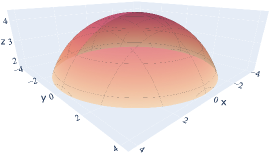
(a) $G_{1}$, $\kappa=0.227$

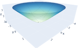
(b) $G_{2}$, $\kappa=-0.536$

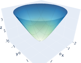
(c) $G_{3}$, $\kappa=-1.073$

Figure 2: Illustration of the Riemannian spaces in the task graphs $G_{t}$ on ogbn-arXiv. $\kappa$ is the learnt curvature.

Related Work

Continual Graph Learning.

Existing studies can be roughly divided into three categories, i.e., replay (or rehearsal), regularization and architectural methods (Febrinanto et al. 2022). Replay methods retrain representative samples in the memory or pseudo-samples to survive from catastrophic forgetting, e.g., ERGNN (Zhou and Cao 2021) introduces a well-designed strategy to select the samples. HPN (Zhang, Song, and Tao 2022) extends knowledge with the prototypes learnt from old tasks. Regularization methods append a regular term to the loss to preserve the utmost past knowledge, e.g., TWP (Liu, Yang, and Wang 2021) preserves important parameters for both task-related and topology-related goals. MSCGL (Cai et al. 2022) is designed for multimodal graphs with neural architectural search. DyGRAIN (Kim, Yun, and Kang 2022) explores the adaptation of receptive fields while distilling knowledge. Architectural methods modify the neural architecture of graph model itself, such as FGN (Wang et al. 2022). Meanwhile, continual graph learning has been applied to recommendation system (Xu et al. 2020), trafficflow prediction (Chen, Wang, and Xie 2021), etc. In addition, Wang et al. (2020) mainly focus on a related but different problem with the time-incremental setting. Recently, Tan et al. (2022); Lu et al. (2022) study the few-shot class-incremental learning on graphs which owns essentially different setting to ours. Since no existing work is suitable for the self-supervised continual graph learning, we are devoted to bridging this gap in this work.

Riemannian Representation Learning.

It has achieved great success in a variety of applications (Mathieu et al. 2019; Gulcehre et al. 2019; Nagano et al. 2019; Sun et al. 2020). Here, we focus on Riemannian models on graphs. In hyperbolic space, Nickel and Kiela (2017); Suzuki, Takahama, and Onoda (2019) introduce shallow models, while HGCN (Chami et al. 2019), HGNN (Liu, Nickel, and Kiela 2019) and LGNN (Zhang et al. 2021) generalize convolutional network with different formalism under static setting. Recently, HVGNN (Sun et al. 2021) and HTGN (Yang et al. 2021) extend hyperbolic graph neural network to temporal graphs. Beyond hyperbolic space, Sala et al. (2018) study the matrix manifold of Riemannian spaces. $\kappa$-GCN (Bachmann, Bécigneul, and Ganea 2020) extends GCN to constant-curvature spaces with $\kappa$-sterographical model, but its formalism cannot be applied to our problem. Yang et al. (2022) model the graph in the dual space of Euclidean and hyperbolic ones. Gu et al. (2019) and Wang et al. (2021) explore the mixed-curvature spaces, and Sun et al. (2022b) propose the first self-supervised GNN in mixed-curvature spaces. Law (2021) and Xiong et al. (2022) study graph learning on a kind of pseudo Riemannian manifold, ultrahyperbolic space. Recently, Sun et al. (2022a) propose a novel GNN in general on Riemannian manifolds with the time-varying curvature. All existing Riemannian models adopt offline training, and we propose the first continual graph learner in Riemannian space to the best of our knowledge.

Conclusion

In this paper, we propose the first self-supervised continual graph learner in adaptive Riemannian spaces, RieGrace. Specifically, we first formulate a unified GNN coupled with the CurvNet, so that Riemannian space is shaped by the learnt curvature adaptive to each task graph. Then, we propose Label-free Lorentz Distillation approach to consolidate knowledge without catastrophic forgetting, where we perform contrastive distillation in Riemannian spaces with the proposed GLP. Extensive experiments on the benchmark datasets show the superiority of RieGrace.

References

- Bachmann, Bécigneul, and Ganea (2020) Bachmann, G.; Bécigneul, G.; and Ganea, O. 2020. Constant Curvature Graph Convolutional Networks. In Proceedings of ICML, volume 119, 486–496.
- Cai et al. (2022) Cai, J.; Wang, X.; Guan, C.; Tang, Y.; Xu, J.; Zhong, B.; and Zhu, W. 2022. Multimodal Continual Graph Learning with Neural Architecture Search. In Proceedings of The ACM Web Conference 2022 (WWW), 1292–1300. ACM.
- Chami et al. (2019) Chami, I.; Ying, Z.; Ré, C.; and Leskovec, J. 2019. Hyperbolic graph convolutional neural networks. In Advances in NeurIPS, 4869–4880.
- Chen et al. (2022) Chen, W.; Han, X.; Lin, Y.; Zhao, H.; Liu, Z.; Li, P.; Sun, M.; and Zhou, J. 2022. Fully Hyperbolic Neural Networks. In Proceedings of ACL, 5672–5686. Association for Computational Linguistics.
- Chen, Wang, and Xie (2021) Chen, X.; Wang, J.; and Xie, K. 2021. TrafficStream: A Streaming Traffic Flow Forecasting Framework Based on Graph Neural Networks and Continual Learning. In Zhou, Z., ed., Proceedings of IJCAI, 3620–3626. ijcai.org.
- Cruceru, Bécigneul, and Ganea (2021) Cruceru, C.; Bécigneul, G.; and Ganea, O. 2021. Computationally Tractable Riemannian Manifolds for Graph Embeddings. In Proceedings of AAAI, 7133–7141. AAAI Press.
- Dragon (2012) Dragon, N. 2012. The Lorentz Group, 123–137. Berlin, Heidelberg: Springer Berlin Heidelberg.
- Febrinanto et al. (2022) Febrinanto, F. G.; Xia, F.; Moore, K.; Thapa, C.; and Aggarwal, C. 2022. Graph Lifelong Learning: A Survey. CoRR, abs/2202.10688.
- Galke et al. (2021) Galke, L.; Franke, B.; Zielke, T.; and Scherp, A. 2021. Lifelong Learning of Graph Neural Networks for Open-World Node Classification. In Proceedings of IJCNN, 1–8. IEEE.
- Gu et al. (2019) Gu, A.; Sala, F.; Gunel, B.; and Ré, C. 2019. Learning Mixed-Curvature Representations in Product Spaces. In Proceedings of ICLR, 1–21.
- Gulcehre et al. (2019) Gulcehre, C.; Denil, M.; Malinowski, M.; Razavi, A.; Pascanu, R.; Hermann, K. M.; Battaglia, P.; Bapst, V.; Raposo, D.; Santoro, A.; and de Freitas, N. 2019. Hyperbolic Attention Networks. In Proceedings of ICLR, 1–15.
- Guo et al. (2023) Guo, J.; Shuang, K.; Zhang, K.; Liu, Y.; Li, J.; and Wang, Z. 2023. Learning to Imagine: Distillation-Based Interactive Context Exploitation for Dialogue State Tracking. In Proceedings of AAAI.
- Hamilton, Ying, and Leskovec (2017) Hamilton, W.; Ying, Z.; and Leskovec, J. 2017. Inductive representation learning on large graphs. In Advances in NeurIPS, 1024–1034.
- Hassani and Ahmadi (2020) Hassani, K.; and Ahmadi, A. H. K. 2020. Contrastive Multi-View Representation Learning on Graphs. In Proceedings of ICML, volume 119, 4116–4126.
- Ke et al. (2021) Ke, Z.; Liu, B.; Ma, N.; Xu, H.; and Shu, L. 2021. Achieving Forgetting Prevention and Knowledge Transfer in Continual Learning. In Advances in NeurIPS, 22443–22456.
- Kim, Yun, and Kang (2022) Kim, S.; Yun, S.; and Kang, J. 2022. DyGRAIN: An Incremental Learning Framework for Dynamic Graphs. In Raedt, L. D., ed., Proceedings of IJCAI, 3157–3163. ijcai.org.
- Kipf and Welling (2017) Kipf, T. N.; and Welling, M. 2017. Semi-supervised classification with graph convolutional networks. In Proceedings of ICLR, 1–12.
- Krioukov et al. (2010) Krioukov, D.; Papadopoulos, F.; Kitsak, M.; Vahdat, A.; and Boguná, M. 2010. Hyperbolic geometry of complex networks. Physical Review E, 82(3): 036106.
- Lange et al. (2022) Lange, M. D.; Aljundi, R.; Masana, M.; Parisot, S.; Jia, X.; Leonardis, A.; Slabaugh, G. G.; and Tuytelaars, T. 2022. A Continual Learning Survey: Defying Forgetting in Classification Tasks. IEEE Trans. Pattern Anal. Mach. Intell., 44(7): 3366–3385.
- Law (2021) Law, M. 2021. Ultrahyperbolic Neural Networks. In Advances in Neural Information Processing Systems, volume 34, 22058–22069.
- Law et al. (2019) Law, M. T.; Liao, R.; Snell, J.; and Zemel, R. S. 2019. Lorentzian Distance Learning for Hyperbolic Representations. In Proceedings of ICML, volume 97, 3672–3681. PMLR.
- Li and Hoiem (2018) Li, Z.; and Hoiem, D. 2018. Learning without Forgetting. IEEE Trans. Pattern Anal. Mach. Intell., 40(12): 2935–2947.
- Liu, Yang, and Wang (2021) Liu, H.; Yang, Y.; and Wang, X. 2021. Overcoming Catastrophic Forgetting in Graph Neural Networks. In Proceedings of AAAI, 8653–8661. AAAI Press.
- Liu, Nickel, and Kiela (2019) Liu, Q.; Nickel, M.; and Kiela, D. 2019. Hyperbolic graph neural networks. In Advances in NeurIPS, 8228–8239.
- Lopez-Paz and Ranzato (2017) Lopez-Paz, D.; and Ranzato, M. 2017. Gradient Episodic Memory for Continual Learning. In Guyon, I.; von Luxburg, U.; Bengio, S.; Wallach, H. M.; Fergus, R.; Vishwanathan, S. V. N.; and Garnett, R., eds., Advances in NeurIPS, 6467–6476.
- Lu et al. (2022) Lu, B.; Gan, X.; Yang, L.; Zhang, W.; Fu, L.; and Wang, X. 2022. Geometer: Graph Few-Shot Class-Incremental Learning via Prototype Representation. In Proceedings of KDD.
- Mathieu et al. (2019) Mathieu, E.; Le Lan, C.; Maddison, C. J.; Tomioka, R.; and Teh, Y. W. 2019. Continuous Hierarchical Representations with Poincaré Variational Auto-Encoders. In Advances in NeurIPS, 12544–12555.
- Mikolov et al. (2013) Mikolov, T.; Sutskever, I.; Chen, K.; Corrado, G. S.; and Dean, J. 2013. Distributed Representations of Words and Phrases and their Compositionality. In Advances in NeurIPS, 3111–3119.
- Nagano et al. (2019) Nagano, Y.; Yamaguchi, S.; Fujita, Y.; and Koyama, M. 2019. A wrapped normal distribution on hyperbolic space for gradient-based learning. In Proceedings of ICML, 4693–4702.
- Nickel and Kiela (2017) Nickel, M.; and Kiela, D. 2017. Poincaré embeddings for learning hierarchical representations. In Advances in NeurIPS, 6338–6347.
- Oord, Li, and Vinyals (2018) Oord, A. v. d.; Li, Y.; and Vinyals, O. 2018. Representation Learning with Contrastive Predictive Coding. arXiv: 1807.03748, 1–13.
- Qiu et al. (2020) Qiu, J.; Chen, Q.; Dong, Y.; Zhang, J.; Yang, H.; Ding, M.; Wang, K.; and Tang, J. 2020. GCC: Graph Contrastive Coding for Graph Neural Network Pre-Training. In Proceedings of KDD, 1150–1160.
- Sala et al. (2018) Sala, F.; Sa, C. D.; Gu, A.; and Ré, C. 2018. Representation Tradeoffs for Hyperbolic Embeddings. In Proceedings of ICML, volume 80, 4457–4466. PMLR.
- Sen et al. (2008) Sen, P.; Namata, G.; Bilgic, M.; Getoor, L.; Gallagher, B.; and Eliassi-Rad, T. 2008. Collective Classification in Network Data. AI Mag., 29(3): 93–106.
- Skopek, Ganea, and Bécigneul (2020) Skopek, O.; Ganea, O.; and Bécigneul, G. 2020. Mixed-curvature Variational Autoencoders. In Proceedings of ICLR, 1–54.
- Sun et al. (2022a) Sun, L.; Ye, J.; Peng, H.; and Yu, P. S. 2022a. A Self-supervised Riemannian GNN with Time Varying Curvature for Temporal Graph Learning. In Proceedings of the 31st CIKM, 1827–1836. ACM.
- Sun et al. (2022b) Sun, L.; Zhang, Z.; Ye, J.; Peng, H.; Zhang, J.; Su, S.; and Yu, P. S. 2022b. A Self-Supervised Mixed-Curvature Graph Neural Network. In Proceedings of AAAI, 4146–4155. AAAI Press.
- Sun et al. (2020) Sun, L.; Zhang, Z.; Zhang, J.; Wang, F.; Du, Y.; Su, S.; and Yu, P. S. 2020. Perfect: A Hyperbolic Embedding for Joint User and Community Alignment. In Proceedings of the 20th ICDM, 501–510. IEEE.
- Sun et al. (2021) Sun, L.; Zhang, Z.; Zhang, J.; Wang, F.; Peng, H.; Su, S.; and Yu, P. S. 2021. Hyperbolic Variational Graph Neural Network for Modeling Dynamic Graphs. In Proceedings of AAAI, 4375–4383. AAAI Press.
- Suzuki, Takahama, and Onoda (2019) Suzuki, R.; Takahama, R.; and Onoda, S. 2019. Hyperbolic Disk Embeddings for Directed Acyclic Graphs. In Proceedings of ICML, 6066–6075.
- Tan et al. (2022) Tan, Z.; Ding, K.; Guo, R.; and Liu, H. 2022. Graph Few-shot Class-incremental Learning. In Proceedings of WSDM, 987–996. ACM.
- Tang et al. (2009) Tang, J.; Sun, J.; Wang, C.; and Yang, Z. 2009. Social influence analysis in large-scale networks. In Proceedings of KDD, 807–816. ACM.
- Tian, Krishnan, and Isola (2020) Tian, Y.; Krishnan, D.; and Isola, P. 2020. Contrastive Representation Distillation. In Proceedings of ICLR, 1–19.
- Veličković et al. (2018) Veličković, P.; Cucurull, G.; Casanova, A.; Romero, A.; Liò, P.; and Bengio, Y. 2018. Graph Attention Networks. In Proceedings of ICLR, 1–12.
- Veličković et al. (2019) Veličković, P.; Fedus, W.; Hamilton, W. L.; Liò, P.; Bengio, Y.; and Hjelm, R. D. 2019. Deep Graph Infomax. In Proceedings of ICLR, 1–24.
- Wang et al. (2022) Wang, C.; Qiu, Y.; Gao, D.; and Scherer, S. 2022. Graph Lifelong Learning. In Proceedings of CVPR, 1–12.
- Wang et al. (2020) Wang, J.; Song, G.; Wu, Y.; and Wang, L. 2020. Streaming Graph Neural Networks via Continual Learning. In Proceedings of CIKM, 1515–1524. ACM.
- Wang et al. (2021) Wang, S.; Wei, X.; dos Santos, C. N.; Wang, Z.; Nallapati, R.; Arnold, A. O.; Xiang, B.; Yu, P. S.; and Cruz, I. F. 2021. Mixed-Curvature Multi-Relational Graph Neural Network for Knowledge Graph Completion. In Proceedings of The ACM Web Conference (WWW), 1761–1771. ACM / IW3C2.
- Weber, Saucan, and Jost (2017) Weber, M.; Saucan, E.; and Jost, J. 2017. Characterizing complex networks with Forman-Ricci curvature and associated geometric flows. J. Complex Networks, 5(4): 527–550.
- Wu et al. (2019) Wu, F.; Jr., A. H. S.; Zhang, T.; Fifty, C.; Yu, T.; and Weinberger, K. Q. 2019. Simplifying Graph Convolutional Networks. In Proceedings of ICML, volume 97, 6861–6871. PMLR.
- Xiong et al. (2022) Xiong, B.; Zhu, S.; Nayyeri, M.; Xu, C.; Pan, S.; Zhou, C.; and Staab, S. 2022. Ultrahyperbolic Knowledge Graph Embeddings. In Proceedings of KDD, 2130–2139. ACM.
- Xu et al. (2020) Xu, Y.; Zhang, Y.; Guo, W.; Guo, H.; Tang, R.; and Coates, M. 2020. GraphSAIL: Graph Structure Aware Incremental Learning for Recommender Systems. In Proceedings of CIKM, 2861–2868. ACM.
- Yang et al. (2022) Yang, H.; Chen, H.; Pan, S.; Li, L.; Yu, P. S.; and Xu, G. 2022. Dual Space Graph Contrastive Learning. In Proceedings of The ACM Web Conference (WWW), 1238–1247.
- Yang et al. (2021) Yang, M.; Zhou, M.; Kalander, M.; Huang, Z.; and King, I. 2021. Discrete-time Temporal Network Embedding via Implicit Hierarchical Learning in Hyperbolic Space. In Proceedings of KDD, 1975–1985. ACM.
- Yin et al. (2022) Yin, Y.; Wang, Q.; Huang, S.; Xiong, H.; and Zhang, X. 2022. AutoGCL: Automated Graph Contrastive Learning via Learnable View Generators. In Proceedings of AAAI, 8892–8900. AAAI Press.
- Yu et al. (2022) Yu, L.; Pei, S.; Ding, L.; Zhou, J.; Li, L.; Zhang, C.; and Zhang, X. 2022. SAIL: Self-Augmented Graph Contrastive Learning. In Proceedings of AAAI, 8927–8935. AAAI Press.
- Zhang, Song, and Tao (2022) Zhang, X.; Song, D.; and Tao, D. 2022. Hierarchical Prototype Networks for Continual Graph Representation Learning. IEEE Transactions on Pattern Analysis and Machine Intelligence, Early Access: 1–15.
- Zhang et al. (2021) Zhang, Y.; Wang, X.; Shi, C.; Liu, N.; and Song, G. 2021. Lorentzian Graph Convolutional Networks. In Proceedings of WWW, 1249–1261.
- Zhou and Cao (2021) Zhou, F.; and Cao, C. 2021. Overcoming Catastrophic Forgetting in Graph Neural Networks with Experience Replay. In Proceedings of AAAI, 4714–4722. AAAI Press.