Interaction-aware Model Predictive Control for Autonomous Driving

Abstract

Lane changing and lane merging remains a challenging task for autonomous driving, due to the strong interaction between the controlled vehicle and the uncertain behavior of the surrounding traffic participants. The interaction induces a dependence of the vehicles’ states on the (stochastic) dynamics of the surrounding vehicles, increasing the difficulty of predicting future trajectories. Furthermore, the small relative distances cause traditional robust approaches to become overly conservative, necessitating control methods that are explicitly aware of inter-vehicle interaction. Towards these goals, we propose an interaction-aware stochastic model predictive control (MPC) strategy integrated with an online learning framework, which models a given driver’s cooperation level as an unknown parameter in a state-dependent probability distribution. The online learning framework adaptively estimates the surrounding vehicle’s cooperation level with the vehicle’s past trajectory and combines this with a kinematic vehicle model to predict the probability of a multimodal future state trajectory. The learning is conducted with logistic regression which enables fast online computation. The multi-future prediction is used in the MPC algorithm to compute the optimal control input while satisfying safety constraints. We demonstrate our algorithm in an interactive lane changing scenario with drivers in different randomly selected cooperation levels.

I INTRODUCTION

The development of autonomous vehicles has been a long-standing endeavour of research and industry due to its potentially far-reaching implications on safety and efficiency of our traffic. Despite significant advances towards this goal, one of the key remaining challenges is the problem of control and planning in close vicinity to surrounding traffic participants. The main sources for these challenges are (i) the inherent uncertainty about the intentions of surrounding drivers (ii) the interaction between the behavior of these drivers and that of the controlled vehicle. To address these issues, we propose a stochastic model for human driving behavior in a highway driving scenario, in which the human driver is assumed to repeatedly make a selection out of a finite set of base policies according to a (a priori unknown) probability distribution. In order to model interactive behavior, we will pose the natural assumption that this distribution depends on the joint state of the involved vehicles (e.g., relative positions and velocities). We describe a simple, online scheme for estimating the dependence of the aforementioned probability distribution on the state and include this model in a chance-constrained stochastic MPC (MPC) formulation, which can be solved effectively over a scenario tree.

I-A Related Work

I-A1 Modeling uncertainty

Existing approaches to MPC under uncertainty on surrounding vehicle motion have can be broadly categorized into robust [1] and stochastic approaches, where the former assumes potentially adversarial behavior of surrounding vehicles, which is accounted for under worst-case assumptions and the latter assumes a stochastic description of the driving behavior, where the expected value of the cost is minimized subject to potentially probabilistic constraints [2]. More recently, risk-averse [3, 4, 5, 6] and distributionally robust [7, 8, 9, 10, 11, 12, 13] approaches have become increasingly popular as they generalize the aforementioned approaches, by accounting for uncertainty in the distribution of the stochastic prediction model.

Most of these existing methods, however, consider the uncertainty to be fully exogenous — the probability distribution does not depend on the state or inputs of the controlled vehicle. This tends to result in reactive and overly conservative behavior (cf. the frozen robot problem [14]).

I-A2 Modeling interaction

A variety of approaches has been proposed to include the interactive behavior in the controller design. Reinforcement learning is applied in [15, 16] to learn an interaction-aware policy directly from data. These methods require little expert knowledge and can typically handle complicated scenarios. However, the resulting policies are usually not easy to introspect, making it difficult to ensure safety or predict failure cases. Furthermore, their quality hinges on the availability of large-scale high-quality datasets.

An alternative approach is to combine MPC with predictive models that describe inter-vehicle interaction. The benefit of this approach is that MPC simultaneously allows for a wide range of expressive dynamical models and furthermore directly accounts for safety restrictions through constraints in the optimal control problem.

Several different interaction-aware MPC formulations have been proposed in recent years, such as game-theoretical MPC [17, 18, 19, 20], where each road user is assumed to behave optimally according to some known or estimated cost function.

A more direct approach is to learn the interactive dynamics through supervised learning [21, 22], where given current states of each vehicle, a trained neural network predicts their future trajectories in a prediction time horizon. Both methods considers uni-modal prediction where the prediction is based on most likely scenario or a predefined policy.

As mentioned before, our goal is to additionally account for the inherent uncertainty in the driving behavior, by considering a stochastic interaction model. Our model class is similar to [23]. However, in [23], the (state-dependent) distribution is assumed to be known, whereas we integrate a procedure for adapting a model for these distributions during operation. Simiarly, [24] integrates MPC with an online learning technique for a similar use case. However, in [24], human driving behavior is modeled as a weighted sum (with unknown weights) of random policies with known distributions, which depends on an estimate of the human driver’s action-value function (i.e., their long-term costs as a function of the current state and control action). Instead, we assume that the human driver will select one of the predefined number of base policies according to an unknown, state-dependent distribution. This only requires knowledge of these base policies corresponding to possible maneuvers, which provides a very direct and intuitive way of modeling possible behaviors for a given traffic scenario. Furthermore, our formulation allows to reduce excessive conservatism through chance constraints, which allows to discard extremely unlikely scenarios. However, [24] presents an indirect dual adaptive control method for active learning, which could be applicable to the model considered in our work. We leave a more thorough investigation of this possibility for future work.

I-B Contribution

We tackle a lane change control problem by utilizing SMPC (SMPC) [25], where we optimize the control input under a finite number of scenarios under decision-dependent uncertainty. Each scenario is defined with a maneuver-based prediction model [26]. In the machine learning literature, this model class is also known as multi-future prediction [27, 28]. Different from [29, 30], we explicitly consider interaction by introducing a state-dependent distribution. Our contribution is twofold: (i) We integrate our MPC method with a simple learning framework which, during operation, adapts the probabilistic interaction model to the current neighboring driver. (ii) We present SMPC SMPC method with a smooth, safe approximation of the (originally non-smooth) chance constraints.

Notation

Let $\left\lVert x\right\rVert_{2}$ denote the Euclidean norm of vector $x$ and $\left\lVert x\right\rVert_{A}^{2}{}\mathop{\mathrel{:}=}{}x^{\top}\!Ax$ for a positive definite matrix $A\succ 0$. We use $\mathbf{diag}\left\{{x}\right\}$ to represent a diagonal matrix with diagonal elements equal to the entries of vector $x$. Given a set $C\subseteq{\rm I\mathchoice{}{}{}{}R}^{n}$, $\mathds{1}_{C}:{\rm I\mathchoice{}{}{}{}R}\ni x\mapsto\mathds{1}_{C}(x)\in{\rm I\mathchoice{}{}{}{}R}$ denotes the function that maps $x$ to 1 when $x\in C$ and to 0 otherwise. $U[a,b]$ represents the uniform distribution defined on the closed interval $[a,b]\subset{\rm I\mathchoice{}{}{}{}R}$ . $\mathcal{N}(\mu,\Sigma)$ denotes the normal distribution with mean $\mu$ and covariance matrix $\Sigma$. Furthermore, for $a<b\in{\rm I\mathchoice{}{}{}{}N}$, we denote ${\rm I\mathchoice{}{}{}{}N}_{[a,b]}{}\mathop{\mathrel{:}=}{}\{k\mid a\leq k\leq b\}$. We denote by $\Delta_{d}{}\mathop{\mathrel{:}=}{}\{p\in{\rm I\mathchoice{}{}{}{}R}^{d}_{+}\mid\sum_{i=1}^{d}p_{i}=1\}$ the $d$-dimensional probability simplex. We denote by $\|A\|_{\mathrm{F}}$ the Frobenius norm of the matrix $A$.

II Modeling and Problem Formulation

Consider a traffic scenario on a highway, consisting of a controlled vehicle (the ego vehicle), referred to by the identifier e, and a number of surrounding road vehicles. The task of the ego vehicle is to safely perform a lane-change maneuver to a lane which is occupied by other road users. At the time of initiating the lane change procedure, we consider the nearest vehicle approaching from the rear in the adjacent lane, which we refer to as the target vehicle, and identify with the index tv. Since the behavior of this agent determines whether the lane change can be safely carried out, we will explicitly model the interaction dynamics with this vehicle, and assume that remaining obstacles can be handled using simplified models.

II-A Vehicle Dynamics

We model all vehicle dynamics with a kinematic bicycle model [31], illustrated in Fig. 1. Let $p=\left[\begin{smallmatrix}p_{x}&p_{y}\end{smallmatrix}\right]^{\top}\in{\rm I\mathchoice{}{}{}{}R}^{2}$ describe the position of the center of gravity expressed in a fixed inertial frame, $\psi$ is the orientation of the vehicle, and $v$ is the velocity of the center of gravity. Its control inputs are the acceleration $a$ and the steering angle $\delta$.

Figure 1: Illustration of the kinematic bicycle model.

The continuous time dynamics are given as

$$\dot{p}_{x}= \;v\cos(\psi+\beta)$$ (1a)

$$\dot{p}_{y}= \;v\sin(\psi+\beta)$$ (1b)

$$\dot{v}= \;a$$ (1c)

$$\dot{\psi}= \;\tfrac{v}{l_{\mathrm{r}}}\sin\beta$$ (1d)

where $$\beta$$ is the slip angle at the center of gravity:

$$\beta= \;\arctan\Big{(}\tfrac{l_{\mathrm{r}}}{l_{\mathrm{f}}+l_{\mathrm{r}}}\tan\delta\Big{)}.$$ (1e)

Denoting the state of vehicle $z{}\mathop{\mathrel{:}=}{}\left[\begin{smallmatrix}p_{x}&p_{y}&v&\psi\end{smallmatrix}\right]^{\top}\in{\rm I\mathchoice{}{}{}{}R}^{4}$ and the control action $u{}\mathop{\mathrel{:}=}{}\left[\begin{smallmatrix}a&\delta\end{smallmatrix}\right]^{\top}\in{\rm I\mathchoice{}{}{}{}R}^{n_{u}}$ ($n_{u}=2$), we discretize (1) using the forward Euler method to obtain a discrete-time system consistent with the simulator we used in the experiments, which we compactly denote as

$$z_{k+1}=f(z_{k},u_{k}).$$ (2)

For ease of notation, we will denote the state of the ego vehicle and the target vehicle as $z^{\textsc{e}}$ and $z^{\textsc{tv}}$, respectively, and we define the concatenated state $\bm{z}{}\mathop{\mathrel{:}=}{}\left(z^{\textsc{e}},z^{\textsc{tv}}\right)\in{\rm I\mathchoice{}{}{}{}R}^{n_{z}}$ (with $n_{z}=8$).

II-B Target vehicle behavior

Let $(\Omega,\mathcal{F},{\rm I\mathchoice{}{}{}{}P})$ be a probability space with countably infinite sample space $\Omega$, $\sigma$-algebra $\mathcal{F}$ and probability measure ${\rm I\mathchoice{}{}{}{}P}:\mathcal{F}\to[0,1]$. We model the uncertain behavior of a given target vehicle as a randomized control policy $\kappa^{\textsc{tv}}:{\rm I\mathchoice{}{}{}{}R}^{n_{z}}\times\Xi\to{\rm I\mathchoice{}{}{}{}R}^{2}$, where $\Xi{}\mathop{\mathrel{:}=}{}\{1,\dots,d\}$ is a finite set corresponding to a number of discrete maneuvers that a driver may perform. We assume that every time step $t$, the selection of the maneuver $\xi_{t}\in\Xi$ is made randomly according to a distribution

$$P\left(\bm{z}_{t}\right)=({\rm I\mathchoice{}{}{}{}P}\{\xi_{t}=i\mid\bm{z}_{t}\})_{i\in\Xi},$$ (3)

which depends on the (combined) state $\bm{z}_{t}$ of the vehicles at time $t$. This state-dependent distribution $P:{\rm I\mathchoice{}{}{}{}R}^{n_{z}}\to\Delta_{d}$ will typically differ between different drivers, and can therefore not easily be estimated offline using traditional methods. Instead, we propose a simple online estimation scheme to estimate this distribution online; This is described in Section III-A. Thus, at a given time $t$, the control action of the target vehicle is a random variable

$$u^{\textsc{tv}}_{t}=\kappa^{\textsc{tv}}\left(\bm{z}_{t},\xi_{t}\right),\quad\xi_{t}\sim P(\bm{z}_{t}),$$

which, combined with (2) results in an autonomous, stochastic system $z^{\textsc{tv}}_{t+1}=f^{\textsc{tv}}\left(\bm{z}_{t},\xi_{t}\right){}\mathop{\mathrel{:}=}{}f\left(z^{\textsc{tv}}_{t},\kappa^{\textsc{tv}}\left(\bm{z}_{t},\xi_{t}\right)\right),$ describing the target vehicle motion. For ease of notation, we combine the dynamics of the ego vehicle and the target vehicle, and introduce $\overline{f}:{\rm I\mathchoice{}{}{}{}R}^{n_{z}}\times{\rm I\mathchoice{}{}{}{}R}^{n_{u}}\to{\rm I\mathchoice{}{}{}{}R}^{n_{z}}$

$$\bm{z}_{t+1}=\overline{f}(\bm{z}_{t},u_{t},\xi_{t}){}\mathop{\mathrel{:}=}{}\left[\begin{smallmatrix}f\left(z^{\textsc{e}}_{t},u_{t}\right)\\ f^{\textsc{tv}}(\bm{z}_{t},\xi_{t})\end{smallmatrix}\right].$$ (4)

(i) The model uncertainty is concentrated in the behavior, resulting in a restriction to dynamically feasible predicted trajectories (ii) The choice of considering a fixed number of known policies allows the designer to incorporate a large amount of known structure about the use case at hand into the target vehicle’s behavioral model (iii) The model is similar to the popular technique of using motion primitives[26], but by using a control policy for the closed-loop model, the predicted trajectories automatically get corrected online using feedback (iv) In contrast to similar models in which the distribution of $(\xi_{t})_{t}$ is state-independent, e.g., [12], the proposed model grants considerably more freedom in modeling interaction between vehicles, since the probability of choosing a certain maneuver typically depends on the relative positions and velocities of nearby vehicles.

II-C Objective Function

We use the usual quadratic stage cost $\ell:{\rm I\mathchoice{}{}{}{}R}^{n_{z}}\times{\rm I\mathchoice{}{}{}{}R}^{n_{u}}\to{\rm I\mathchoice{}{}{}{}R}_{+}$,

$$\ell(\bm{z},u){}\mathop{\mathrel{:}=}{}\|z^{\textsc{e}}-z^{\mathrm{ref}}\|^{2}_{Q}+\|u^{\textsc{e}}\|^{2}_{R},$$ (5)

where $Q\succeq 0$ and $R\succ 0$ are given weights for the ego vehicle’s states and inputs, respectively, and $z^{\mathrm{ref}}$ is a given reference state.

II-D Input and state constraints

II-D1 Simple state and input bounds

As usual in control applications, we will assume there are hard limits on both the states and the inputs, which we will write as

$$u_{t}\in U,\bm{z}_{t}\in Z,\forall t\in{\rm I\mathchoice{}{}{}{}N},$$

where $U\subseteq{\rm I\mathchoice{}{}{}{}R}^{n_{u}},Z\in{\rm I\mathchoice{}{}{}{}R}^{n_{z}}$ are given, nonempty, closed sets. Since we are only actively controlling the ego vehicle, we will typically take $Z=Z^{\textsc{e}}\times{\rm I\mathchoice{}{}{}{}R}^{4}$, with $Z^{\textsc{e}}$ a given constraint set for the ego vehicle state. In practice, both $Z^{\textsc{e}}$ and $U$ will often be simple component-wise upper and lower bounds.

II-D2 Slew rate constraints

To ensure comfortable driving behavior and account for unmodeled actuator dynamics, it is common to include slew-rate constraints of the form

$$|u_{k}-u_{k-1}|\leq\epsilon_{\delta_{u}},$$

where the absolute values and inequality are taken element-wise, and $\epsilon_{\delta_{u}}>0$ is a given constant.

II-E Collision Avoidance

Given a vehicle with current state $z=\left[\begin{smallmatrix}p&v&\psi\end{smallmatrix}\right]^{\top}$, with $p\in{\rm I\mathchoice{}{}{}{}R}^{2}$, we – similarly to, e.g., [32] – approximate the area it occupies as the union of $n_{\mathrm{c}}=3$ circles with radius $r=\tfrac{1}{2}\sqrt{(\nicefrac{{l}}{{n_{\mathrm{c}}}})^{2}+w^{2}}$ and centers

$$c_{j}\left(z\right){}\mathop{\mathrel{:}=}{}p+\tfrac{l}{2n_{\mathrm{c}}}\left(2j-n_{\mathrm{c}}-1\right)\left[\begin{smallmatrix}\cos\psi\\ \sin\psi\end{smallmatrix}\right],\quad j=1,\dots,n_{\mathrm{c}},$$

as illustrated in Fig. 2.

A sufficient condition for collision avoidance between the vehicles e and tv, with respective states $z^{\textsc{e}}$ and $z^{\textsc{tv}}$, is then

$$g_{ij}\left(\bm{z}\right){}\mathop{\mathrel{:}=}{}4r^{2}-\|c_{i}(z^{\textsc{e}})-c_{j}(z^{\textsc{tv}})\|_{2}^{2}\leq 0,\quad\forall i,j\in[n_{\mathrm{c}}].$$ (6)

Note that the functions $g_{ij}:{\rm I\mathchoice{}{}{}{}R}^{n_{z}}\to{\rm I\mathchoice{}{}{}{}R}$ smooth, yet concave, and will thus lead to nonconvex constraints.

Figure 2: Illustration of the collision avoidance constraints.

Very often, the distribution $P\left(\bm{z}\right)$ will be concentrated on a small subset of $\Xi$. For instance, whenever the ego vehicle drives directly in front of the target vehicle. The probability that the target vehicle will heavily accelerate, causing a rear-end collision, will be very low. Imposing collision avoidance constraint (6) for the predicted states under this scenario, would be unreasonably conservative and would in many cases simply lead to infeasibility. To resolve this issue, we will instead aim to impose (6) probabilistically. More specifically, at any time step $t$, our goal is to impose

$${\rm I\mathchoice{}{}{}{}P}\{\max_{i,j\in[n_{\mathrm{c}}]}g_{ij}\left(\bm{z}_{t+1}\right)\leq 0\mid\bm{z}_{t}\}\geq 1-\gamma,$$

for a given violation rate $\gamma\in[0,1)$. By definition (3), this constraint depends on the state-dependent maneuver distribution $P$.

II-F Nominal optimal control problem

We are now ready to formulate the stochastic optimal control problem, which we ideally would like to solve in a receding horizon fashion to obtain an interaction-aware MPC scheme for the described task. As we will see, however, this problem cannot be solved directly. Instead, Section III is dedicated to proposing suitable approximations to the formulations, resulting in a practical control scheme.

Let $\Pi{}\mathop{\mathrel{:}=}{}\{\mu_{k}:{\rm I\mathchoice{}{}{}{}R}^{n_{z}}\to{\rm I\mathchoice{}{}{}{}R}^{n_{u}},k\in{\rm I\mathchoice{}{}{}{}N}_{[0,N-1]}\}$ denote the set of all causal $N$-step control policies.

Given an initial state $\overline{\bm{z}}$, combine the introduced elements to obtain obtain the (idealized) stochastic optimal control problem

$$\operatorname*{minimize}_{(\mu_{t})_{t}\in\Pi} {\rm I\mathchoice{}{}{}{}E}_{\xi}\Big{\{}\sum_{k=0}^{N-1}\ell(\bm{z}_{k},u_{k})+\ell_{N}\left(\bm{z}_{N}\right)\mid\bar{\bm{z}}\Big{\}}$$ (7a)

$$\;\operatorname*{s.t.} \bm{z}_{0}=(z^{\textsc{e}}_{0},z^{\textsc{tv}}_{0})=\bar{\bm{z}},$$ (7b)

$$z^{\textsc{e}}_{k+1}=f(z^{\textsc{e}}_{k},u_{k}),u_{k}=\mu_{k}\left(\bm{z}_{k}\right),$$ (7c)

$$z^{\textsc{tv}}_{k+1}=f^{\textsc{tv}}\big{(}z^{\textsc{tv}}_{k},\xi_{k}\big{)},$$ (7d)

$${\rm I\mathchoice{}{}{}{}P}\big{\{}\max_{i,j\in[n_{\mathrm{c}}]}g_{ij}(\bm{z}_{k+1}){}\leq{}0\mid\bm{z}_{k}\big{\}}\geq 1-\gamma,$$ (7e)

$$u_{k}\in U,\;\bm{z}_{k}\in Z,\bm{z}_{N}\in Z,\,\mathrm{a.s.},$$ (7f)

$$|u_{k^{\prime}+1}-u_{k^{\prime}}|\leq\epsilon_{\delta_{u}}\,\mathrm{a.s.},$$ (7g)

$$\forall k\in{\rm I\mathchoice{}{}{}{}N}_{[0,N-1]},\;\forall k^{\prime}\in{\rm I\mathchoice{}{}{}{}N}_{[0,N-2]},$$

where the qualifier $a.s.$ (almost surely) indicates that the constraint must hold in all realizations that occur with nonzero probability. Of course, as it is stated here, this problem is intractable due to (i) the infinite-dimensional decision variables $(\mu_{k})_{k}$ (ii) the distribution $P$ governing the stochastic process $(\xi_{k})_{k}$ (cf. (3)) being unknown (iii) the non-smooth chance constraint (7e). In the next section, we will propose an approximate formulation of (7), addressing these difficulties and resulting in an implementable control scheme.

III Interaction-Aware MPC

III-A Learning the distribution

The state-dependent distribution $P$ introduced in (3) is not known in advance, and furthermore, it cannot be accurately estimated offline, as it may vary significantly between drivers. This necessitates the introduction of an online learning method.

To this end, we use a simple multinomial logistic regression scheme, where we introduce a parameterized model $\hat{P}:{\rm I\mathchoice{}{}{}{}R}^{n_{z}}\times{\rm I\mathchoice{}{}{}{}R}^{n_{\theta}\times d}\to{\rm I\mathchoice{}{}{}{}R}^{d}$

$$\hat{P}\left(\bm{z};\theta\right){}\mathop{\mathrel{:}=}{}\bigg{(}\frac{\exp(\theta_{i}^{\top}\varphi(\bm{z}))}{\sum_{j=1}^{d}\exp(\theta_{i}^{\top}\varphi(\bm{z}))}\bigg{)}_{i=1}^{d}$$ (8)

where $\varphi:{\rm I\mathchoice{}{}{}{}R}^{n_{z}}\to{\rm I\mathchoice{}{}{}{}R}^{n_{\theta}}:\bm{z}\mapsto\left(\varphi_{i}\left(\bm{z}\right)\right)_{i=1}^{n_{\theta}}$, is a vector-valued feature function, with $\varphi_{1}\equiv 1$, which accounts for the bias term, and $\theta=\left[\begin{smallmatrix}\theta_{1}&\dots&\theta_{d}\end{smallmatrix}\right]\in{\rm I\mathchoice{}{}{}{}R}^{n_{\theta}\times d}$ is the parameter matrix.

III-A1 Maximum-likelihood estimation

Given a dataset $D_{T}{}\mathop{\mathrel{:}=}{}\left(\bm{z}_{k},\xi_{k}\right)_{k=1}^{T}$, the parameter $\theta$ is determined by maximizing the log-likelihood [33, §4.4]:

$$\theta^{\star}\in\operatorname*{\arg\!\min}_{\theta}-\textstyle\sum_{k=1}^{T}\log\hat{P}_{\xi_{k}}\big{(}\varphi(\bm{z}_{k});\theta\big{)}.$$ (9)

If $D_{T}$ is obtained offline from a collection of different drivers, then it may be used to obtain an initial guess for the driving parameters of a new driver. However, since $\theta$ may vary significantly from one driver to another, we additionally consider an online procedure for updating $\theta$ for the currently neighboring target vehicle.

III-A2 Online Learning

In order to adapt the parameter with measurements obtained during operation, we use a moving horizon estimation update. At every time step $t$, we compute a new estimate

$$\theta_{t}\in\operatorname*{\arg\!\min}_{\theta}\lambda\rho(\theta,\theta_{t-1})-\sum_{k=t-L+1}^{t}\log\hat{P}_{\xi_{k}}\big{(}\bm{z}_{k};\theta\big{)},$$ (10)

where $L\in{\rm I\mathchoice{}{}{}{}N}$ is a fixed window length, $\lambda>0$ is a fixed regularization constant and $\rho:\left(\theta,\theta^{\prime}\right)\mapsto\|\theta-\theta^{\prime}\|_{\mathrm{F}}^{2}$ penalizes large differences between $\theta$ and the previous estimate $\theta_{t-1}$.

III-B Chance constraint approximation

We now move our attention to obtaining approximate reformulations of the problem (7), which can be effectively solved online within MPC MPC scheme.

Let us first consider the chance constraint (7e). Given a random quantity $\zeta:\Xi\to{\rm I\mathchoice{}{}{}{}R}$, we may write

$${\rm I\mathchoice{}{}{}{}P}\{\zeta(\xi_{k})>0\mid\bm{z}_{k}\}=\sum_{\xi\in\Xi}P_{\xi}(\bm{z}_{k})\mathds{1}_{{\rm I\mathchoice{}{}{}{}R}_{+}}(\zeta(\xi_{k})).$$ (11)

The function $\mathds{1}_{{\rm I\mathchoice{}{}{}{}R}_{+}}$ is nonconvex, and furthermore, it is discontinuous at 0, making it unsuitable for numerical optimization. To remedy this, we aim to replace it by a continuous and/or smooth approximation. A common choice for such a surrogate function is the average value-at-risk ($\operatorname{AVaR}$) [34], which results in the smallest convex upper approximation of the original chance constraint. However, it may be rather conservative, in particular in the case where the number of outcomes, i.e., $|\Xi|=d$, is small, as we illustrate in Example 1. Due to the collision avoidance constraints and the nonlinear dynamics, (7a) is nonconvex irrespective of the surrogate used for $\mathds{1}_{{\rm I\mathchoice{}{}{}{}R}_{+}}$. Obtaining a convex upper approximation is therefore of limited value. Instead, we replace the right-hand side of (11) by

$$\sum_{\xi\in\Xi}P_{\xi}(\bm{z}_{k})\mathds{1}_{{\rm I\mathchoice{}{}{}{}R}_{+}}(\zeta(\xi_{k}))\leq\sum_{\xi\in\Xi}P_{\xi}(\bm{z}_{k})\sigma(\zeta(\xi_{k})),$$ (12)

where

$$\sigma(x)=\tfrac{a}{1+\exp\left(-\alpha(x-\overline{x}\right))}$$ (13)

is the sigmoid function with parameters $a>0$ $\alpha>0$, $\overline{x}$. The larger the $\alpha$, the more accurate the approximation (12) can be made, at the cost of larger gradients and curvature, which tend to impede convergence of numerical solvers. The parameters $a$ or $\overline{x}$ can be selected such that the inequality $\sigma\geq\mathds{1}_{{\rm I\mathchoice{}{}{}{}R}_{+}}$ (and therefore (12)) is satisfied uniformly by solving $\sigma(0)=1$. The remaining parameter can be freely selected, e.g., to obtain the least conservative estimate. In Section IV, we simply select $a$ and $\alpha$ as tuning parameters and select $\overline{x}$ to satisfy (12).

We illustrate the potential benefit of using the sigmoid approximation over the popular $\operatorname{AVaR}$ approximation using a simple example.

Example 1 (Comparison with $\operatorname{AVaR}$)

Figure 3: Comparison between approximations $\nu$ of the indicator function $\mathbf{1}_{{\rm I\mathchoice{}{}{}{}R}_{+}}$ in the case of Example 1. The blue histogram (left axis) represents the probability mass function of a random quantity $\zeta$; The green curves (right axis) represent $\mathbf{1}_{{\rm I\mathchoice{}{}{}{}R}_{+}}$ and its upper bounds corresponding to $\operatorname{AVaR}$ and the sigmoid approximation (12).

Consider a random variable $\zeta:\Omega\to{\rm I\mathchoice{}{}{}{}R}$, represented by the discrete outcomes $(\zeta_{i})_{i=1}^{4}$ (uniformly spaced between -5 and 2), with probabilities $({\rm I\mathchoice{}{}{}{}P}\{\zeta=\zeta_{i}\})_{i=1}^{4}=\left[\begin{smallmatrix}0.6&0.3&0.08&0.02\end{smallmatrix}\right]$, as illustrated in Fig. 3. Suppose that our goal is to ensure ${\rm I\mathchoice{}{}{}{}P}\{\zeta>0\}\leq\gamma=0.05$. It is clear from the set-up that ${\rm I\mathchoice{}{}{}{}P}\{\zeta>0\}=0.02$ in this case, so $\zeta$ satisfies our constraint.

The well-known average value-at-risk is defined as $\operatorname{AVaR}_{\gamma}(\zeta){}\mathop{\mathrel{:}=}{}\min_{t\in{\rm I\mathchoice{}{}{}{}R}}t+\tfrac{1}{\gamma}{\rm I\mathchoice{}{}{}{}E}\{[\zeta-t]_{+}\},$ with minimizer $t^{\star}$. Then, through the change of variables $c^{\star}=-\nicefrac{{1}}{{t^{\star}}}$, it can be shown that the condition $\operatorname{AVaR}_{\gamma}(\zeta)\leq 0$ is equivalent to ${\rm I\mathchoice{}{}{}{}E}\{[1+c^{\star}\zeta]_{+}\}\leq\gamma$ [35, §6.2.4]. Thus, $\operatorname{AVaR}$ can be interpreted as an approximation of the form (12), but with a piecewise-affine upper bound for the indicator $\mathds{1}_{{\rm I\mathchoice{}{}{}{}R}_{+}}$. This is shown in Fig. 3 for this particular example of $\zeta$. The compared approximations of the violation probability are thus given as $\sum_{i=1}^{4}p_{i}\nu(\zeta_{i})$, for $\nu\in\{[1+c^{\star}(\,\cdot\,)]_{+},\sigma\}$, resulting in $0.14$ and $0.037$, for $\operatorname{AVaR}$ and $\sigma$, respectively. Notice that due to the large slope $c^{\star}$ obtained for the $\operatorname{AVaR}$ approximation, the value of the largest (highly unlikely) realization of $\zeta$ is heavily overweighed, resulting in an overapproximation of the constraint violation rate by a factor 7, compared to a factor 1.85 for the sigmoid approximation with $\alpha=10$, $a=1.33$, $\overline{x}=-0.11$.

III-C Optimal control over scenario trees

III-C1 Scenario tree notation

Figure 4: A fully branching scenario tree of horizon $N=2$.

Consider an arbitrary $N$-step policy $(\mu_{k})_{k=0}^{N-1}\in\Pi$. Since $\Xi=\{1,\dots,d\}$ is a finite set, all realizations of the stochastic process $(\bm{z}_{k},u_{k})_{k=1}^{N}$ satisfying (4) with $u_{k}=\mu_{k}\left(\bm{z}_{k}\right)$, and $\bm{z}_{0}$ known can be represented on a scenario tree [36] as illustrated in Fig. 4.

A scenario tree is a tree with a unique root node (with index 0) representing the current time step. For all possible outcomes of $\xi_{0}$, a new node is connected to node 0. The result is a set of nodes representing the outcomes of the process at time $1$. Repeating this process $N$ times results in a tree, whose nodes are partitioned into $N+1$ time steps, or stages. We denote the set of all nodes at stage $k\in{\rm I\mathchoice{}{}{}{}N}_{[0,N]}$ by $\operatorname*{nod}(k)$. By extension, given $a<b\in{\rm I\mathchoice{}{}{}{}N}_{[0,N]}$, we denote $\operatorname*{nod}\left(a,b\right)=\bigcup_{k=a}^{b}\operatorname*{nod}(k)$. For a given node $\iota\in\operatorname*{nod}(k)$, $k\in{\rm I\mathchoice{}{}{}{}N}_{[1,N]}$, we denote its ancestor as $\operatorname*{anc}{\iota}\in\operatorname*{nod}(k-1)$. Conversely, we define the children of $\iota\in\operatorname*{nod}\left(k\right)$, $k\in{\rm I\mathchoice{}{}{}{}N}_{[0,N-1]}$ as $\operatorname*{ch}(\iota){}\mathop{\mathrel{:}=}{}\{j\in\operatorname*{nod}(k+1)\mid\operatorname*{anc}(j)=\iota\}$. A node $\iota\in\operatorname*{nod}(N)$ for which $\operatorname*{ch}(\iota)=\emptyset$ is called a leaf node. Each leaf node $\iota$ corresponds to a scenario $\operatorname*{scen}(\iota){}\mathop{\mathrel{:}=}{}\{\iota_{k}\in\operatorname*{nod}(k)\}_{k=0}^{N}$ with $\iota_{k-1}=\operatorname*{anc}(\iota_{k}),\forall k\in{\rm I\mathchoice{}{}{}{}N}_{[1,N]}$, which represents a single realization of the underlying stochastic process over $N$ future time steps. We denote a variable $z$ associated to a node $\iota\in\operatorname*{nod}\left(0,N\right)$ as $z^{(\iota)}$, as illustrated in Fig. 4.

III-C2 Optimal control problem

Using this structure, we can represent the $N$-step policy $(\mu_{k})_{k=0}^{N-{1}}\in\Pi$ (cf. (7)) by a collection $\bm{u}{}\mathop{\mathrel{:}=}{}\left(u^{(\iota)}\right)_{\iota\in\operatorname*{nod}\left(0,N-1\right)}\in{\rm I\mathchoice{}{}{}{}R}^{n_{u}M}$ of finite-dimensional control vectors. Here, $M{}\mathop{\mathrel{:}=}{}|\operatorname*{nod}\left(0,N-1\right)|$ is the number of non-leaf nodes in the scenario tree. Accordingly, the stochastic dynamics (4) can be represented in scenario tree notation as

$$\bm{z}^{(\iota)}=\overline{f}(\bm{z}^{(\operatorname*{anc}{\iota})},u^{(\operatorname*{anc}{\iota})},\xi^{(\iota)}).$$ (14)

Now we may decompose the control objective (7a) as follows. For a given parameter (estimate) $\theta$, let $\hat{P}\left(\;\cdot\;,\theta\right)=\big{(}\hat{P}_{\xi}(\;\cdot\;,\theta)\big{)}_{\xi\in\Xi}$ denote our estimate of the distribution $P$, as obtained from (8)–(10). Then, for each leaf node $s\in\operatorname*{nod}(N)$, the estimated probability of its associated scenario is given as

$$\bar{P}_{s}\big{(}\bm{u},\theta\big{)}{}\mathop{\mathrel{:}=}{}\hskip 5.0pt\prod_{\mathclap{\iota\in\operatorname*{scen}\left(s\right)\setminus\{0\}}}\hat{P}_{\xi^{(\iota)}}(\bm{z}^{(\operatorname*{anc}{\iota})},\theta),$$ (15)

where the predicted state $\bm{z}^{(\iota)}$ in node $\iota\in\operatorname*{nod}\left(0,N-1\right)$, can be expressed as a function of $\bm{u}$ and the known initial state $\bm{z}^{(0)}$ using (14). (We omitted the dependence on $\bm{z}^{(0)}$ to ease notation.) Using (15), the expected cost (7a) can be expressed on the scenario tree as the function $J_{N}:{\rm I\mathchoice{}{}{}{}R}^{n_{u}M}\to{\rm I\mathchoice{}{}{}{}R}_{+}$

$$J_{N}\left(\bm{u},\theta\right){}\mathop{\mathrel{:}=}{}\>\sum_{\mathclap{s\in\operatorname*{nod}(N)}}\bar{P}_{s}(\bm{u},\theta)\Big{(}\ell_{N}(\bm{z}^{(s)}){}+{}\sum_{\mathclap{\begin{subarray}{c}\iota\in\operatorname*{scen}(s)\\ \setminus{\operatorname*{nod}{(N)}}\end{subarray}}}\ell(\bm{z}^{(\iota)},u^{(\iota)})\Big{)}.$$

Combining these ingredients, we obtain our reformulated optimal control problem: Given $\bm{\bar{z}}$, and $\theta$,

$$\operatorname*{minimize}_{\bm{u}\in{\rm I\mathchoice{}{}{}{}R}^{n_{u}M}} J_{N}(\bm{u},\theta)$$ (16a)

$$\operatorname*{s.t.} z^{(0)}=\bar{\bm{z}},$$ (16b)

$$\bm{z}^{(\iota_{+})}=\overline{f}\big{(}\bm{z}^{(\iota)},u^{(\iota)},\xi^{(\iota_{+})}\big{)}\;\forall\iota_{+}\in\operatorname*{ch}{\iota},$$ (16c)

$$\smashoperator[l]{\sum_{\iota_{+}\in\operatorname*{ch}{\iota}}^{}}\hat{P}_{\iota_{+}}(z^{(\iota)},\theta)\sigma_{\alpha}\Big{(}\overline{g}\big{(}\bm{z}^{(\iota_{+})}\big{)}\Big{)}\leq\gamma,$$ (16d)

$$u^{(\iota)}_{k}\in U,\;\bm{z}^{(\iota)}_{k}\in Z,$$ (16e)

$$\bm{z}^{(\iota_{N})}\in Z,\;\forall\iota_{N}\in\operatorname*{nod}{N},$$ (16f)

$$|u^{(\iota_{+})}-u^{(\iota)}|\leq\epsilon_{\delta_{u}}\;\forall\iota_{+}\in\operatorname*{ch}{\iota},$$ (16g)

$$\forall\iota\in\operatorname*{nod}(0,N-1),$$ (16h)

where $\overline{g}(z){}\mathop{\mathrel{:}=}{}\max_{k,l\in{\rm I\mathchoice{}{}{}{}N}_{[1,n_{\mathrm{c}}]}}g_{kl}(z)$. In practice, we avoid this pointwise-maximum and further approximate (16d) using the union bound. In particular:

1. If node $\iota$ has more than one child node, we approximate $\sigma\Big{(}\overline{g}\big{(}\bm{z}^{(\iota_{+})}\big{)}\Big{)}$ with $\sum_{k,l\in{\rm I\mathchoice{}{}{}{}N}_{[1,n_{\mathrm{c}}]}}\sigma\Big{(}g_{kl}\big{(}\bm{z}^{(\iota_{+})}\big{)}\Big{)}$;

2. If node $\iota$ has only one child, i.e., $\operatorname*{ch}(\iota)=\{\iota_{+}\}$, constraint (7e) reduces to $g_{kl}(z^{\iota_{+}})\leq 0\;\;\forall k,l\in{\rm I\mathchoice{}{}{}{}N}_{[1,n_{\mathrm{c}}]}$.

This problem is a standard nonlinear problem, which can be solved with off-the-shelf numerical solvers.

III-C3 Scenario tree approximations

It is clear that number of scenarios in the tree grows exponentially with the prediction horizon. Several techniques exist to combat this explosive growth while maintaining a sufficiently long prediction horizon for planning complex tasks. For instance, in [37], a scenario tree is dynamically built by repeatedly adding the most likely child node to any of the current leaf nodes, until a desired number of nodes is reached. However, this approach is not directly applicable in our setting, since the transition probabilities are not yet available when constructing the tree, as they depend on the future states over which we need to optimize.

$(N,N_{\mathrm{b}},D)=(8,2,1)$

$(N,N_{\mathrm{b}},D)=(8,4,2)$

$(N,N_{\mathrm{b}},D)=(8,8,4)$

Figure 5: Different combinations of the branching horizon $N_{\mathrm{b}}$ and timescale factor $D$ leading to an approximate scenario tree of horizon $N$, each with the same number of scenarios.

More direct approaches (illustrated in Fig. 5) involve a combination of the following: (i) Fix a branching horizon $N_{\mathrm{b}}<N$, after which the modes are kept constant, i.e., set $\xi_{k}=\xi_{k-1}$ for all $k>N_{\mathrm{b}}$ [12] (ii) assume that the discrete process $(\xi_{t})_{t\in{\rm I\mathchoice{}{}{}{}N}}$ governing the branching, evolves at a slower timescale than the continuous state updates. That is, assume that $\xi_{k}\sim P\left(\bm{z}_{k}\right)$ if $k\mod D=0$, otherwise, $\xi_{k}=\xi_{k-1}$ [23]. In general, the most suitable choice depends on the particular application. We have found that for our use case, the resulting behavior is very similar in both cases.

IV Numerical experiments

We illustrate the proposed control method on a simple lane-change scenario, using the highway-env [38] simulator.

IV-A Interactive Target Vehicle Behavior

TABLE I: Target vehicle parameters

Symbol	Description	Value
$a_{\textrm{comf}}$	maximum comfort acceleration	3 [$\text{\,}\mathrm{m}\mathrm{/}\mathrm{s}^{2}$]
$k_{\texttt{b}},\;k_{\texttt{t}}$	control gain in maneuver	0.7 [-]
$N_{\mathrm{p}}$	P-IDM prediction horizon	$U[0.1,1]$ [$\text{\,}\mathrm{s}$]
$c_{\mathrm{thres}}$	Decision threshold	$U[0,4]$ [$\text{\,}\mathrm{m}$]

IV-A1 Maneuvers

For simplicity, we will assume the target vehicle only moves in the longitudinal direction. Lateral motion is handled internally by the simulator. We consider two base policies, represented by the set $\Xi=\{\texttt{brake},\texttt{track}\}$. That is, we assume that the (stochastic) target vehicle policy is given as $\kappa^{\textsc{tv}}(\bm{z},\xi)=\left[\begin{smallmatrix}\max\{a_{\mathrm{min}},\min\{a_{\textrm{comf}},a^{\textsc{tv}}(\bm{z},\xi)\}\}&0\end{smallmatrix}\right]^{\top}$ with

$$a^{\textsc{tv}}(\bm{z},\xi)=\begin{cases}-k_{b}v^{\textsc{tv}}&\text{if}\quad\xi=\texttt{brake}\\ k_{t}(v_{\max}-v^{\textsc{tv}})&\text{if}\quad\xi=\texttt{track}.\end{cases}$$

IV-A2 Interaction model

Following the Predictive Intelligent Driver Model (P-IDM) [39], the target vehicle will predict the ego vehicle’s trajectory with constant velocity to make decisions. If (i) $p_{x}^{\textsc{e}}>p_{x}^{\textsc{tv}}$ (ii) $\exists k\in{\rm I\mathchoice{}{}{}{}N}_{[0,N_{\mathrm{p}}]}:\;\big{|}p_{y,k}^{\textsc{e}}-p_{y,k}^{\textsc{tv}}\big{|}\leq c_{\mathrm{thres}}$ the target vehicle will choose brake. Otherwise it chooses track. The prediction horizon $N_{\mathrm{p}}$ and the threshold $c_{\mathrm{thres}}$ may differ per individual driver. Note that this behavior can be captured quite well using the proposed probabilistic model (8).

IV-B Simulation Results and Analysis

We consider a straight two-lane highway. Each vehicle is modeled as a box with a length of $5\text{\,}\mathrm{m}$ and a width of $2\text{\,}\mathrm{m}$.

IV-B1 Simulation overview

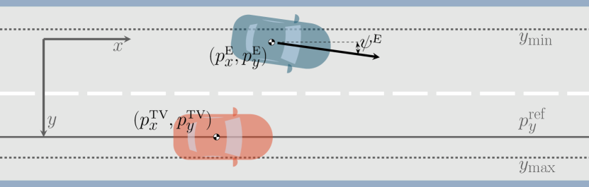
Figure 6: Illustration of the coordinate system.

The goal of ego vehicle is to drive in the center of the right lane at the maximum velocity, i.e., the reference state in (5) is $z^{\mathrm{ref}}=(0,p_{y}^{\mathrm{ref}},v^{\mathrm{ref}},0)$ (cf. Table II). The coordinate system is illustrated in Fig. 6. The two vehicles are initialized on two adjacent lanes with random relative distance $p_{x,0}^{\textsc{e}}-p_{x,0}^{\textsc{tv}}\sim U[0,5]$\text{\,}\mathrm{m}$$, $p_{y,0}=p_{y,0}^{\textsc{e}}-p_{y,0}^{\textsc{tv}}\sim U[-5,-3]$\text{\,}\mathrm{m}$$. Over all experiments, the ego vehicle has fixed longitudinal initial position $p_{x,0}^{\textsc{e}}=$6\text{\,}\mathrm{m}$$ and the target vehicle has fixed lateral initial position $p_{y,0}^{\textsc{tv}}=$4\text{\,}\mathrm{m}$$. The initial velocities are drawn randomly as $v_{0}^{\textsc{e}},v_{0}^{\textsc{tv}}\sim U[23,25]$\text{\,}\mathrm{m}\mathrm{/}\mathrm{s}$$. The hyperparameters and constraints used in the simulation are summarized in Table II. As described in §III-C3, we control the scenario tree complexity by selecting branching horizon $N_{\mathrm{b}}=11$ and timescale factor $D=5$.

TABLE II: MPC parameters

Symbol	Description	Value
$T_{\mathrm{s}}$	sampling time	$0.1\text{\,}\mathrm{s}$
$T_{\mathrm{sim}}$	simulation horizon	$6\text{\,}\mathrm{s}$
$Q$	weights for states	$\mathbf{diag}\left\{{0,1,0.01,\nicefrac{{16}}{{\pi^{2}}}}\right\}$
$R$	weights for input	$\mathbf{diag}\left\{{0.01,\nicefrac{{16}}{{\pi^{2}}}}\right\}$
$N$	prediction horizon	20
$r_{c}$	circle radius in (6)	$1.3\text{\,}\mathrm{m}$
$(\alpha,a)$	parameters in (13)	(10, 1.2)
$\gamma$	threshold in (16d)	0.05
$L$	window length in (10)	15
$\lambda$	weight in (10)	1
$[y_{\min},y_{\max}]$	bounds on lateral position	$[-1,5]$\text{\,}\mathrm{m}$$
$[v_{\min},v_{\max}]$	bounds on velocity	$[0,28]$\text{\,}\mathrm{m}\mathrm{/}\mathrm{s}$$
$[\psi_{\min},\psi_{\max}]$	bounds on heading angle	$[-\nicefrac{{\pi}}{{4}},\nicefrac{{\pi}}{{4}}]$\text{\,}\mathrm{rad}$$
$[a_{\mathrm{min}},a_{\mathrm{max}}]$	bounds on acceleration	$[-5,5]$\text{\,}\mathrm{m}\mathrm{/}\mathrm{s}^{2}$$
$[\delta_{\min},\delta_{\max}]$	bounds on steering angle	$[-\nicefrac{{\pi}}{{4}},\nicefrac{{\pi}}{{4}}]$\text{\,}\mathrm{rad}$$
$\epsilon_{\delta_{u}}$	bounds on slew rate (16h)	$[5,\nicefrac{{\pi}}{{4}}]$

We compare the following variants of the method:

1. MLE: Estimate $\theta_{t}$ according to (10), with $\theta_{0}=0$;

2. MLE-P: Estimate $\theta_{t}$ according to (10), with $\theta_{0}=\hat{\theta}$ obtained according to Section IV-B2;

3. PRIOR: Use the prior $\hat{\theta}$ without online learning;

4. EMP: Replace the state-dependent distribution by the empirical distribution $\hat{P}_{t}=\big{(}t^{-1}\sum_{j=0}^{t-1}\mathds{1}_{\{i\}}(\xi_{j})\big{)}_{i\in\Xi}$ with $t$ the current time step of the simulation;

5. UNI: Use uniform distribution $\hat{P}_{t}=(0.5,0.5)$, $\forall t\in{\rm I\mathchoice{}{}{}{}N}$;

6. BRA: Assume $\xi_{t}=\texttt{brake}$, i.e., $\hat{P}_{t}=(1,0)$, $\forall t\in{\rm I\mathchoice{}{}{}{}N}$;

7. TRA: Assume $\xi_{t}=\texttt{track}$, i.e., $\hat{P}_{t}=(0,1)$, $\forall t\in{\rm I\mathchoice{}{}{}{}N}$.

Each method is simulated 50 times with random initial states and target vehicle parameters. The problem (16) is implemented with CasADi [40] and solved using Ipopt [41]. After the first step, the solver is warm-started with a shifted version of the previous solution. If the problem is infeasible with warm-starting, it is resolved with zero as initial guess. The convex parameter estimation problem (10) is solved using Mosek[42] through Cvxpy [43].

IV-B2 Offline parameter estimation

An informative initial guess $\hat{\theta}$ for the parameter is estimated from a synthetic offline dataset containing 800 training points and 200 validation points generated from 10 different drivers. We solve (9) to obtain (8) with feature function $\varphi(\bm{z})=z^{\textsc{e}}-z^{\textsc{tv}}$. The fitted function achieves a misclassification rate of 0.175 on the validation set. We point out that given the same states, different drivers may choose different maneuvers according to their own driving style. Therefore a model with zero prediction error is not expected.

IV-B3 Results and analysis

A snapshot of successful lane-changing is presented in Fig. 7.

Figure 7: Snapshot of a closed-loop simulation. The ego vehicle and target vehicle are shown in blue and yellow, respectively. The last 5 time steps are shown as transparent rectangles and the predicted trajectories are shown as lines

The control performance is quantified with closed-loop cost. The simulation result presented in Table III demonstrates the advantage of employing the decision-dependent distribution instead of a fixed distribution, and furthermore, MLE-P estimator performs the best on average. This shows the benefit of obtaining an informative prior estimate. On the other hand, without informative prior, online learning can efficiently capture the driver behavior and reaches better level control performance than only using offline approximated distribution. In addition, no collision occurs in the simulations, which proves the effectiveness of our collision avoidance constraint formulation.

TABLE III: Simulation results. If the ego vehicle is sufficiently close to the reference¹, we record the relative positive of ego vehicle to the target vehicle (front / behind). Otherwise we categorize the run under ‘time-out’.

	number of simulations				closed-loop cost
method	collision	front	behind	time-out	mean	Q3${}^{\hyperlink{Q3}{2}}$
MLE	0	34	5	11	154.31	163.30
MLE-P	0	31	11	8	139.50	161.77
PRIOR	0	25	14	11	157.13	165.11
EMP	0	34	5	11	154.85	160.26
UNI	0	33	5	12	167.89	243.92
BRA	0	33	1	16	186.86	302.64
TRA	0	25	16	9	159.54	211.21

${}^{1}\big{(}\left\lvert p_{y}^{\textsc{e}}-p_{y}^{\mathrm{ref}}\right\rvert\leq 0.1$ and $\left\lvert\psi^{\textsc{e}}-\psi^{\mathrm{ref}}\right\rvert\leq 0.01\big{)}$   ²Third quartile

V Conclusions

We presented a control framework based on SMPC for lane changing problem in autonomous driving, where the interaction was accounted for by modeling the behavior of surrounding vehicles using a stochastic policy with state-dependent distribution. We present an approximate reformulation of the resulting nonlinear, chance-constrained optimal control problem and presented a simple moving horizon scheme for learning the parameters describing the driving style of an adjacent driver. Qualitative and quantitative analysis shows that learning the distribution helps to reduce conservatism of the resulting MPC controller.

References

- [1] A. Bemporad and M. Morari, “Robust model predictive control: A survey,” in Robustness in identification and control. Springer, 1999, pp. 207–226.
- [2] A. Mesbah, “Stochastic model predictive control: An overview and perspectives for future research,” IEEE Control Systems Magazine, vol. 36, no. 6, pp. 30–44, 2016.
- [3] P. Sopasakis, D. Herceg, A. Bemporad, and P. Patrinos, “Risk-averse model predictive control,” Automatica, vol. 100, pp. 281–288, 2019.
- [4] P. Sopasakis, M. Schuurmans, and P. Patrinos, “Risk-averse risk-constrained optimal control,” in 2019 18th European Control Conference (ECC). IEEE, 2019, pp. 375–380.
- [5] M. Schuurmans, A. Katriniok, H. E. Tseng, and P. Patrinos, “Learning-based risk-averse model predictive control for adaptive cruise control with stochastic driver models,” IFAC-PapersOnLine, vol. 53, no. 2, pp. 15 128–15 133, 2020.
- [6] A. Dixit, M. Ahmadi, and J. W. Burdick, “Risk-Averse Receding Horizon Motion Planning,” Apr. 2022.
- [7] M. Schuurmans, P. Sopasakis, and P. Patrinos, “Safe learning-based control of stochastic jump linear systems: a distributionally robust approach,” in 2019 IEEE 58th Conference on Decision and Control (CDC). IEEE, 2019, pp. 6498–6503.
- [8] M. Schuurmans and P. Patrinos, “Learning-based distributionally robust model predictive control of markovian switching systems with guaranteed stability and recursive feasibility,” in 2020 59th IEEE Conference on Decision and Control (CDC). IEEE, 2020, pp. 4287–4292.
- [9] P. Coppens, M. Schuurmans, and P. Patrinos, “Data-driven distributionally robust lqr with multiplicative noise,” in Learning for Dynamics and Control. PMLR, 2020, pp. 521–530.
- [10] M. Schuurmans and P. Patrinos, “Data-driven distributionally robust control of partially observable jump linear systems,” in 2021 60th IEEE Conference on Decision and Control (CDC). IEEE, 2021, pp. 4332–4337.
- [11] P. Coppens and P. Patrinos, “Data-driven distributionally robust mpc for constrained stochastic systems,” IEEE Control Systems Letters, vol. 6, pp. 1274–1279, 2021.
- [12] M. Schuurmans, A. Katriniok, C. Meissen, H. E. Tseng, and P. Patrinos, “Safe, Learning-Based MPC for Highway Driving under Lane-Change Uncertainty: A Distributionally Robust Approach,” Nov. 2022.
- [13] M. Schuurmans and P. Patrinos, “A general framework for learning-based distributionally robust mpc of markov jump systems,” arXiv preprint arXiv:2106.00561, 2021.
- [14] P. Trautman and A. Krause, “Unfreezing the robot: Navigation in dense, interacting crowds,” in 2010 IEEE/RSJ International Conference on Intelligent Robots and Systems. Taipei: IEEE, Oct. 2010, pp. 797–803.
- [15] M. Bouton, A. Nakhaei, D. Isele, K. Fujimura, and M. J. Kochenderfer, “Reinforcement learning with iterative reasoning for merging in dense traffic,” in 2020 IEEE 23rd International Conference on Intelligent Transportation Systems (ITSC). IEEE, 2020, pp. 1–6.
- [16] Y. Hu, A. Nakhaei, M. Tomizuka, and K. Fujimura, “Interaction-aware decision making with adaptive strategies under merging scenarios,” in 2019 IEEE/RSJ International Conference on Intelligent Robots and Systems (IROS). IEEE, 2019, pp. 151–158.
- [17] A. Dreves and M. Gerdts, “A generalized Nash equilibrium approach for optimal control problems of autonomous cars,” Optimal Control Applications and Methods, vol. 39, no. 1, pp. 326–342, 2018.
- [18] F. Fabiani and S. Grammatico, “Multi-vehicle automated driving as a generalized mixed-integer potential game,” IEEE Transactions on Intelligent Transportation Systems, vol. 21, no. 3, pp. 1064–1073, 2019.
- [19] S. L. Cleac’h, M. Schwager, and Z. Manchester, “Algames: A fast solver for constrained dynamic games,” arXiv preprint arXiv:1910.09713, 2019.
- [20] B. Evens, M. Schuurmans, and P. Patrinos, “Learning mpc for interaction-aware autonomous driving: A game-theoretic approach,” in 2022 European Control Conference (ECC). IEEE, 2022, pp. 34–39.
- [21] S. Bae, D. Saxena, A. Nakhaei, C. Choi, K. Fujimura, and S. Moura, “Cooperation-aware lane change maneuver in dense traffic based on model predictive control with recurrent neural network,” in 2020 American Control Conference (ACC). IEEE, 2020, pp. 1209–1216.
- [22] K. Liu, N. Li, H. E. Tseng, I. Kolmanovsky, and A. Girard, “Interaction-aware trajectory prediction and planning for autonomous vehicles in forced merge scenarios,” arXiv preprint arXiv:2112.07624, 2021.
- [23] Y. Chen, U. Rosolia, W. Ubellacker, N. Csomay-Shanklin, and A. D. Ames, “Interactive Multi-Modal Motion Planning With Branch Model Predictive Control,” IEEE Robotics and Automation Letters, vol. 7, no. 2, pp. 5365–5372, Apr. 2022.
- [24] H. Hu and J. F. Fisac, “Active uncertainty learning for human-robot interaction: An implicit dual control approach,” arXiv preprint arXiv:2202.07720, 2022.
- [25] P. Patrinos, P. Sopasakis, H. Sarimveis, and A. Bemporad, “Stochastic model predictive control for constrained discrete-time markovian switching systems,” Automatica, vol. 50, no. 10, pp. 2504–2514, 2014.
- [26] S. Lefèvre, D. Vasquez, and C. Laugier, “A survey on motion prediction and risk assessment for intelligent vehicles,” ROBOMECH journal, vol. 1, no. 1, pp. 1–14, 2014.
- [27] Y. Chai, B. Sapp, M. Bansal, and D. Anguelov, “Multipath: Multiple probabilistic anchor trajectory hypotheses for behavior prediction,” arXiv preprint arXiv:1910.05449, 2019.
- [28] H. Cui, V. Radosavljevic, F.-C. Chou, T.-H. Lin, T. Nguyen, T.-K. Huang, J. Schneider, and N. Djuric, “Multimodal trajectory predictions for autonomous driving using deep convolutional networks,” in 2019 International Conference on Robotics and Automation (ICRA). IEEE, 2019, pp. 2090–2096.
- [29] G. Cesari, G. Schildbach, A. Carvalho, and F. Borrelli, “Scenario model predictive control for lane change assistance and autonomous driving on highways,” IEEE Intelligent transportation systems magazine, vol. 9, no. 3, pp. 23–35, 2017.
- [30] S. H. Nair, V. Govindarajan, T. Lin, Y. Wang, E. H. Tseng, and F. Borrelli, “Stochastic mpc with dual control for autonomous driving with multi-modal interaction-aware predictions,” arXiv preprint arXiv:2208.03525, 2022.
- [31] P. Polack, F. Altché, B. d’Andréa Novel, and A. de La Fortelle, “The kinematic bicycle model: A consistent model for planning feasible trajectories for autonomous vehicles?” in 2017 IEEE intelligent vehicles symposium (IV). IEEE, 2017, pp. 812–818.
- [32] A. Wang, A. Jasour, and B. C. Williams, “Non-Gaussian Chance-Constrained Trajectory Planning for Autonomous Vehicles Under Agent Uncertainty,” IEEE Robotics and Automation Letters, vol. 5, no. 4, pp. 6041–6048, Oct. 2020.
- [33] T. Hastie, R. Tibshirani, J. H. Friedman, and J. H. Friedman, The elements of statistical learning: data mining, inference, and prediction. Springer, 2009, vol. 2.
- [34] A. Nemirovski, “On safe tractable approximations of chance constraints,” European Journal of Operational Research, vol. 219, no. 3, pp. 707–718, June 2012.
- [35] A. Shapiro, D. Dentcheva, and A. Ruszczynski, Lectures on Stochastic Programming: Modeling and Theory, 3rd ed., ser. MOS-SIAM Series on Optimization. Society for Industrial and Applied Mathematics, July 2021.
- [36] G. C. Pflug and A. Pichler, Multistage Stochastic Optimization, ser. Springer Series in Operations Research and Financial Engineering. Cham: Springer International Publishing, 2014.
- [37] D. Bernardini and A. Bemporad, “Stabilizing Model Predictive Control of Stochastic Constrained Linear Systems,” IEEE Transactions on Automatic Control, vol. 57, no. 6, pp. 1468–1480, June 2012.
- [38] E. Leurent, “An environment for autonomous driving decision-making,” https://github.com/eleurent/highway-env, 2018.
- [39] B. Brito, A. Agarwal, and J. Alonso-Mora, “Learning interaction-aware guidance for trajectory optimization in dense traffic scenarios,” IEEE Transactions on Intelligent Transportation Systems, 2022.
- [40] J. A. E. Andersson, J. Gillis, G. Horn, J. B. Rawlings, and M. Diehl, “CasADi – A software framework for nonlinear optimization and optimal control,” Mathematical Programming Computation, vol. 11, no. 1, pp. 1–36, 2019.
- [41] A. Wächter and L. T. Biegler, “On the implementation of an interior-point filter line-search algorithm for large-scale nonlinear programming,” Mathematical programming, vol. 106, no. 1, pp. 25–57, 2006.
- [42] M. ApS, MOSEK Optimizer API for Python 10.0.27, 2022. [Online]. Available: https://docs.mosek.com/10.0/pythonapi/index.html
- [43] S. Diamond and S. Boyd, “CVXPY: A Python-embedded modeling language for convex optimization,” Journal of Machine Learning Research, vol. 17, no. 83, pp. 1–5, 2016.