Effective Emission Heights of Various OH Lines From X-shooter and SABER Observations of a Passing Quasi-2-Day Wave
Abstract
Chemiluminescent radiation of the vibrationally and rotationally excited OH radical, which dominates the nighttime near-infrared emission of the Earth’s atmosphere in wide wavelength regions, is an important tracer of the chemical and dynamical state of the mesopause region between 80 and 100 km. As radiative lifetimes and rate coefficients for collision-related transitions depend on the OH energy level, line-dependent emission profiles are expected. However, except for some height differences for whole bands mostly revealed by satellite-based measurements, there is a lack of data for individual lines. We succeeded in deriving effective emission heights for 298 OH lines thanks to the joint observation of a strong quasi-2-day wave (Q2DW) in eight nights in 2017 with the medium-resolution spectrograph X-shooter at the Very Large Telescope at Cerro Paranal in Chile and the limb-sounding SABER radiometer on the TIMED satellite. Our fitting procedure revealed the most convincing results for a single wave with a period of about 44 h and a vertical wavelength of about 32 km. The line-dependent as well as altitude-resolved phases of the Q2DW then resulted in effective heights which differ by up to 8 km and tend to increase with increasing vibrational and rotational excitation. The measured dependence of emission heights and wave amplitudes (which were strongest after midnight) on the line parameters implies the presence of a cold thermalized and a hot non-thermalized population for each vibrational level.
JGR: Atmospheres
Institut für Physik, Universität Augsburg, Augsburg, Germany Deutsches Fernerkundungsdatenzentrum, Deutsches Zentrum für Luft- und Raumfahrt, Weßling-Oberpfaffenhofen, Germany Institut für Astro- und Teilchenphysik, Universität Innsbruck, Innsbruck, Austria Instituto de Astronomía, Universidad Católica del Norte, Antofagasta, Chile
Stefan Nollstefan.noll@dlr.de
X-shooter-based intensities of 298 OH lines from eight nights show a strong Q2DW in southern summer 2017
Fits of the Q2DW phase in the X-shooter data and SABER-based OH emission profiles were used to derive effective OH emission heights
The line-dependent wave amplitudes confirm the presence of cold and hot OH populations for each vibrational level
Plain Language Summary
Hydroxyl (OH) is an important molecule in the Earth’s atmosphere at altitudes between 80 and 100 km. It is the main source of atmospheric nighttime radiation in the near-infrared wavelength range and is therefore a valuable tracer of the chemistry and dynamics at high altitudes. The emission spectrum consists of various lines which are related to different levels of vibration and rotation. Although the vertical emission distribution should depend on the given line due to differences in the deactivation of the corresponding energy levels, the line-specific details have been uncertain until now. We have succeeded in deriving effective time-averaged emission heights for 298 OH lines based on the combination of ground-based line-resolved and space-based height-resolved observations of a very strong rising wave with a period close to 2 days and a relatively short vertical wavelength in eight nights in 2017. The resulting heights (obtained via the line-dependent wave phases) differ by up to 8 km and generally increase with higher molecular vibration and rotation. They are valuable for ground-based studies of other waves and contribute (combined with conclusions from the wave amplitudes) to a better understanding of the internal processes in OH molecules.
1 Introduction
The nocturnal atmospheric emission of wide wavelength regions in the near-infrared is dominated by chemiluminescent radiation of various roto-vibrational bands up to the vibrational level of the electronic ground state of the hydroxyl (OH) radical [<]e.g.,¿meinel50,noll15,rousselot00. Excited OH is mostly produced by the reaction of hydrogen with ozone [Bates \BBA Nicolet (\APACyear1950)]. The nightglow emission essentially originates from altitudes between 80 and 100 km, and is therefore an important tracer of the chemistry and dynamics in the Earth’s mesopause region. Rocket flights showed typical peak heights of about 87 km and layer widths of about 8 km [Baker \BBA Stair (\APACyear1988)]. Moreover, OH emission profiles have frequently been observed by limb-sounding instruments in space [<]e.g.,¿baker07,dodd94,savigny12,wuest20,yee97. Rare ground-based altitude measurements relied on the identification of the same emission features in imaging instruments at different sites [<]e.g.,¿kubota99,moreels08. \citeAyu17 combined wind observations with a meteor radar and a Fabry-Perot interferometer focusing on OH to estimate peak heights of the radiation. Finally, rough estimates are also possible by means of the well-established negative relation between effective emission height and emission intensity [<]e.g.,¿garcia17,liu06,mulligan09,savigny15,yee97, which can be explained by the larger change of the layer profile at lower altitudes due to the stronger relative variations of atomic oxygen (which is required for the ozone production). The published relations had to be calibrated with satellite observations.
The hydrogen–ozone reaction mainly produces OH populations in high between 7 and 9 [<]e.g.,¿adler97. In contrast, measured populations increase with decreasing [<]e.g.,¿takahashi81,cosby07,noll15. This discrepancy is caused by the step-by-step relaxation process due to the radiation of photons and collisions with other atmospheric constituents [<]e.g.,¿adler97,xu12,noll18b. As the radiative lifetimes and rate coefficients for the collisions with different species depend on the OH level, the resulting emission profiles for individual lines should differ. Models show an increase of the peak emission height with increasing [<]e.g.,¿adler97,makhlouf95,mcdade91,savigny12,xu12. The spread between high and low may amount to several kilometers with possibly larger height shifts for low . Collisions of OH with atomic oxygen appear to be especially crucial for the -dependent discrepancies [von Savigny \BOthers. (\APACyear2012)]. The impact of rotational energy on the altitude distribution has been modeled quite rarely. \citeAdodd94 discussed the differences between populations with rotational quantum numbers up to 7 and those with . Density profiles for the larger appear to peak higher with similar altitude differences as obtained for the comparison of low and high . Moreover, the density peaks seem to show less variation for larger with respect to changes in . \citeAnoll18b presented modeling results for and found maximum -dependent height differences between 1.5 and 2.8 km depending on the uncertain rate coefficients for collisions with atomic oxygen.
Measurements of the impact of the OH energy state on the height distribution were successfully performed with space-based limb sounding. The studies mostly focused on the comparison of the emission profiles of a few roto-vibrational bands [Noll \BOthers. (\APACyear2016), Sheese \BOthers. (\APACyear2014), von Savigny \BBA Lednyts’kyy (\APACyear2013), von Savigny \BOthers. (\APACyear2012)]. The results suggest typical height changes for of about 0.4 to 0.5 km. These differences can vary by a significant fraction of the values. They tend to increase with lower peak altitude and higher atomic oxygen concentration [von Savigny \BBA Lednyts’kyy (\APACyear2013)]. The former can change by several kilometers forced by waves on different time scales and the general circulation [<]e.g.,¿liu06,nikoukar07,noll16,teiser17,yee97. The majority of the variability is found below the emission peak [Nikoukar \BOthers. (\APACyear2007)], where the atomic oxygen density profile is particularly steep. In contrast to whole roto-vibrational bands, there is a lack of studies of individual lines with different . The only noteworthy data known to us are related to observations with the Cryogenic InfraRed Radiance Instrumentation for Shuttle (CIRRIS 1A) Michelson interferometer onboard Space Shuttle Discovery for three days in 1991 [Dodd \BOthers. (\APACyear1994)]. The measured limb profiles comprise lines of several with as well as purely rotational lines with around 15 and 30. However, the interpretation of the data required sophisticated modeling.
There is an alternative approach to estimate effective emission heights of OH lines. Perturbations passing the mesopause region will produce characteristic patterns in the OH intensity time series that will be shifted in time depending on the altitude of the emission [Noll \BOthers. (\APACyear2015), Schmidt \BOthers. (\APACyear2018)]. In this way, the relative layering of different emissions can be obtained from ground-based observations of individual lines. Nevertheless, the derivation of absolute heights will also need information on the vertical propagation of the perturbation through the OH emission layer as can be measured by satellite-based limb-sounding instruments. As the satellites relevant for nightglow observations have nearly Sun-synchronous orbits [<]e.g.,¿russell99,savigny12,yee97, the minimum time scale of the variations needs to be of the order of days for a promising combination of the profile data with ground-based spectra of OH lines in order to link wave phases with altitudes in the same region.
The so-called quasi-2-day wave (Q2DW) can achieve very high amplitudes in the mesopause region at low to middle latitudes. In particular, strong Q2DWs occur in the Southern Hemisphere for several weeks in the summer months January and February [<]e.g.,¿ern13,gu19,tunbridge11,walterscheid15. The period is close to 2 days but can vary from 42 to 54 h [Gu \BOthers. (\APACyear2019)]. For periods very close to 48 h, there can be phase locking with tidal modes [Walterscheid \BBA Vincent (\APACyear1996)]. Southern Q2DWs usually show a dominating westward-moving longitudinal pattern with a zonal wavenumber of 3 (W3), which can be accompanied by other modes with different periods, zonal wavenumbers, and propagation directions [<]e.g.,¿he21,pedatella12,tunbridge11. Q2DWs are regarded to belong to the class of Rossby-gravity waves [<]e.g.,¿salby81. Their genesis is probably related to baroclinic/barotropic instabilities in the summertime easterly zonal wind jet in the lower mesosphere [Plumb (\APACyear1983)], which seem to be linked to increased gravity-wave drag [Ern \BOthers. (\APACyear2013)]. The amplitudes maximize at the OH emission heights and can reach more than 10 K in temperature [Gu \BOthers. (\APACyear2019), Tunbridge \BOthers. (\APACyear2011)] and 50 m s-1 in wind [Limpasuvan \BOthers. (\APACyear2005), Wu \BOthers. (\APACyear1993)]. Between the Q2DW source region and these altitudes at low to middle latitudes, the propagation perpendicular to the zonal component is effectively upward. The situation is different in the lower thermosphere well above the OH layer, where a northward meridional flow tends to be dominant in the Southern Hemisphere [Yue \BOthers. (\APACyear2012)]. At OH emission heights, vertical wavelengths are mostly longer than 20 km and are often even beyond 100 km [Huang \BOthers. (\APACyear2013), Reisin (\APACyear2021)]. The impact of a Q2DW on OH emission was investigated by \citeApedatella12 based on space-based OH profile data for January 2006. The peak emission rate varied by a factor of about 4. This large effect appears to be mostly related to Q2DW-induced variations of the atomic oxygen concentration at the OH emission heights. The concentration can also be modulated by tides and gravity waves.
We have succeeded in deriving effective emission heights for about 300 OH lines by means of the combination of ground-based spectroscopic and space-based height-resolved observations of a strong Q2DW in January to February 2017. The OH line intensities originate from near-infrared spectra of the medium-resolution spectrograph X-shooter [Vernet \BOthers. (\APACyear2011)] of the Very Large Telescope (VLT) of the European Southern Observatory (ESO) at Cerro Paranal in Chile (24.6∘ S, 70.4∘ W). Scans of the OH emission profiles in two filter bands at about 1.6 and 2.1 m are related to measurements with the Sounding of the Atmosphere using Broadband Emission Radiometry (SABER) instrument onboard the Thermosphere Ionosphere Mesosphere Energetics Dynamics (TIMED) satellite [Russell \BOthers. (\APACyear1999)]. In the following section 2, we will describe the data sets for both instruments. Then, we will present our approach to fit the observed wave (section 3). Our results will be shown in section 4, which also includes our estimates of line-dependent effective emission heights (section 4.3) and a brief discussion of another Q2DW in 2019 (section 4.4). Finally, we will draw our conclusions (section 5).
2 Data
2.1 X-shooter
The X-shooter medium-resolution echelle spectrograph [Vernet \BOthers. (\APACyear2011)] mounted at an 8 m telescope of the VLT can simultaneously observe a very wide wavelength range from 0.3 to 2.5 m covered by three spectroscopic arms with separate optical components and detectors. Since the strongest OH bands for all upper vibrational levels from 2 to 9 are found in the near-infrared regime [<]e.g.,¿rousselot00, we focus our analysis on the correspondingly named NIR arm, which extends from 1.0 to 2.5 m. For this arm and scientific targets, the projected slit width can vary between 0.4 and 1.5′′ on the sky, which corresponds to a spectral resolving power between 12,000 and 3,500. The projected slit length is fixed to 11′′.
The spectra used originate from the ESO Science Archive Facility. This study only uses a small fraction of the data that were processed by us. The whole sample comprises about 90,000 spectra in the NIR arm with an exposure time of at least 10 s that were taken between October 2009 and September 2019. The basic processing of the raw echelle spectra was performed by means of the official reduction pipeline [Modigliani \BOthers. (\APACyear2010)] in version v2.6.8 and calibration data preprocessed by ESO [<]see also¿unterguggenberger17. The resulting two-dimensional (2D) wavelength-calibrated sky spectra were subjected to post-processing optimized for the retrieval of airglow emission. First, the 2D spectra were averaged along the spatial direction in order to obtain one-dimensional (1D) spectra. Then, the separation of sky emission and astronomical target performed by the pipeline was improved. For this goal, we extracted residual sky in the 2D object spectrum from the third of the slit positions with the lowest integrated counts in the whole wavelength range. After the minimization of noise by smoothing, we added the resulting 1D mean spectrum to the sky spectrum. This approach was particularly useful for bright star-like astronomical targets.
Although the pipeline produces flux-calibrated spectra, we performed this processing step independently in order to minimize the errors by means of a consistent approach for the entire data set. For the NIR arm, pipeline-processed spectra of the relatively bright spectrophotometric standard stars EG 274 and LTT 3218 [Moehler \BOthers. (\APACyear2014)] were corrected for telluric absorption using a model-based fitting approach [Smette \BOthers. (\APACyear2015), Kausch \BOthers. (\APACyear2015)] and then compared to the theoretical spectral energy distributions in order to derive individual response curves that indicate the wavelength-dependent instrumental quantum efficiency. As the resulting response curves for both stars did not exactly match, we lowered the quantum efficiency of the EG 274 curves (by about 3% in a wide wavelength range) for a better consistency. Thus, remaining systematic uncertainties in the absolute flux calibration for clear sky conditions mainly depend on the quality of the reference spectrum for LTT 3218. As the response curves are relatively uncertain at wavelengths longer than 1.9 m [<]see¿noll15, we used spectra of so-called telluric standard stars with well-known spectral energy distributions (Rayleigh–Jeans law) for atmospheric absorption measurements to derive a general correction function. In order to further improve the quality, master response curves for 10 time periods with lengths between 9 and 15 months were created including only the best-quality data and involving a final smoothing procedure. The splitting of the periods is usually at New Year but also considers a change in the calibration products in January 2013 and a recoating of the main mirror in December 2016. An analysis of the variability of the flux-calibrated star spectra points to relative uncertainties of only 2 to 3% up to 2.1 m in the NIR arm. This is a clear improvement in comparison to a maximum difference in the response of about 12%. The final set of master response curves was applied to the 1D sky spectra. A minor fraction of the spectra were taken with a so-called -blocking filter [Vernet \BOthers. (\APACyear2011)], which reduces the useful wavelength range to wavelengths shorter than 2.1 m. These spectra had to be calibrated with a 1.3 times higher response in order to correctly consider differences in the calibration data.
The measurement of the line intensities was performed in two steps. First, the underlying continuum was determined. After various tests, our procedure used the first quintile of the pixel intensities (cut at 20%) in wavelength ranges with a relative width of 0.008 to derive the continuum at the corresponding central positions. The width was increased by the factors 5.0 and 2.5 around the dense roto-vibrational O2 emission bands at about 1.27 and 1.58 m, respectively [<]e.g.,¿rousselot00. It was multiplied by a factor of 0.4 beyond 2.08 m in order to avoid issues with the steeply increasing continuum due to thermal radiation of the telescope. After subtraction of the resulting continuum, the residual flux was integrated in specific wavelength ranges depending on the central wavelength of the OH doublet, separation of both components [<]e.g.,¿noll20, and slit width. As an X-shooter profile of an unresolved line doublet (which is true in most cases) can be approximated by the combination of a fixed Gaussian and a slit-dependent boxcar, the integration limits had been optimized to assure relatively stable distances to the positions marking half peak intensity. For example, the size of these margins amounts to about 60% of the full integration range minus the doublet separation for the most frequently used slit with a width of 0.9′′. The separation of the integration limits was sufficiently wide to avoid significant flux losses by uncertainties in the wavelength calibration (fraction of a pixel). Positions of suitable lines were taken from \citeAbrooke16. Important selection criteria were clear detectability (at least for long exposures), the lack of blends with other emission lines, a smooth continuum without strong absorption features, and high atmospheric transmission. In the end, the selection procedure (which also included a check for outliers in the scientific analysis) resulted in 298 OH doublets from 14 bands, which cover upper vibrational levels between 2 and 9 and upper rotational levels up to 15.
The measured line intensities were corrected for the van Rhijn effect [van Rhijn (\APACyear1921)], i.e. the projected layer width, assuming a reference altitude of 87 km. The correction of this effect is important as there is a strong variation in the zenith angles of astronomical observations. We also considered the absorption of line emission by molecules in the lower atmosphere in a similar way as decribed by \citeAnoll15. The approach involves the calculation of line-specific transmissions based on the zenith angle, Cerro Paranal atmospheric data [Noll \BOthers. (\APACyear2012)], the Line-By-Line Radiative Transfer Model [<]LBLRTM,¿clough05, and the assumption of purely Doppler-broadened OH lines for a temperature of 190 K at \citeAbrooke16 wavelengths. Transmissions for entire doublets were derived by means of weights for the individual components that were taken from the branch-specific OH level population fits of \citeAnoll20. Reference line transmissions were calculated for zenith and a typical amount of precipitable water vapour (PWV) of 2.5 mm. Doublets with reference transmissions lower than 70% were not considered for the final line set (average of 96%). Differences in the optical depth in the spectroscopic data set were calculated depending on the most crucial parameters, zenith angle and PWV. For the latter, accurate measurements with a Low Humidity And Temperature PROfiler (L-HATPRO) microwave radiometer are available at Cerro Paranal [Kerber \BOthers. (\APACyear2012)]. However, as the L-HATPRO data set starts in 2014 and shows several gaps afterwards, we mostly used these data to calibrate intensity ratios of lines with low and high transmission in the bands OH(2-0) and OH(6-4) to estimate PWV values for each spectrum [<]cf.¿xu20. Up to very high L-HATPRO PWVs of about 16 mm, the approach works quite well with a mean offset of -0.1 mm and a standard deviation of 0.6 mm. With an upper cut at 6 mm (which still represents about 90% of the data), the systematic shift is negligible and the scatter is only half as large.
The quality of the measurement of OH line intensities strongly varies from spectrum to spectrum due to strong changes in spectral resolution, exposure time, atmospheric water vapour, and especially contamination by (spatially extended) astronomical targets that can have a different effect on each line. For this reason, we performed a line-specific selection of suitable observations. Starting with a preselected set of 88,481 useful spectra, we carried out an iterative -clipping procedure for each line. This outlier rejection involved limits with respect to the underlying continuum, the intensity error, and the intensity itself. The error was estimated from the deviation of the residual continuum at both margins of the integration range from the zero line. It was made sure that it was always lower than 10% for the selected measurements. As a result, the line-specific selection rates varied between 69.4% and 99.8% with a mean value of 94.1% for wavelengths shorter than 2.1 m. In order to handle the wide range of exposure times between 10 s and 2.5 h and the corresponding impact on the data quality, we did not use the individual measurements for the analysis. Instead, we divided the 10 years into bins of 30 min, which are sufficiently short for the analysis of Q2DWs. Each bin contains the line-specific spectra with matching central time. The effective intensities were calculated weighted by the exposure time. In the subsequent analysis, we only considered those bins with a summed exposure time of at least 10 min. The average numbers of the selected bins were 19,480 and 17,001 for lines at wavelengths shorter and longer than 2.1 m. A lower minimum exposure time of 5 min did not significantly change the results of the analysis but increased the scatter.
The resulting binned time series were inspected with respect to Q2DW features. The focus was on the months January and February. The X-shooter data set shows a strongly varying time coverage due to the different astronomical observing programs and the usual mounting of two to three instruments at the same telescope, which can cause gaps of the order of weeks. As a consequence, we clearly identified Q2DW events only in the years 2017 and 2019. Moreover, only fractions of the lifetime of a wave were well covered by X-shooter observations. The good intervals are eight nights from 26 January to 3 February 2017 and seven nights from 11 to 18 January 2019. The corresponding maximum numbers of bins of 30 min are 88 and 89, respectively. As the sample of selected spectra is different for each line, up to three bins from 2017 were lost for line wavelengths below 2.1 m. At longer wavelengths, where 30 OH lines are affected by the optional -blocking filter, the bin numbers were 78 and 35 for the years 2017 and 2019, respectively. The comparison of Q2DW results of lines with the same upper levels but different bin numbers did not show any significant discrepancies for the data from 2017. However, the lines at long wavelengths had to be excluded from the analysis of the data from 2019. The drop from 89 to 35 bins was too large.
2.2 SABER
For better understanding the Q2DW-related X-shooter data and adding important altitude-dependent information, we also considered limb-sounding data (version v2.0) of the SABER radiometer on TIMED [Russell \BOthers. (\APACyear1999)]. The observing channels centered on 1.64 and 2.06 m essentially cover emission of the OH(4-2) and OH(5-3) bands as well as the OH(8-6) and OH(9-7) bands [Baker \BOthers. (\APACyear2007)]. Consequently, the effective upper vibrational levels of both channels are about 4.6 and 8.3 [Noll \BOthers. (\APACyear2016)]. We used the so-called “unfiltered” products, i.e. the given volume emission rates (VERs) had been corrected for the missing line emission of the stated OH bands in the wavelength ranges covered by the channels [Mlynczak \BOthers. (\APACyear2005)]. For some checks, we also considered VER profiles of the channel at about 1.27 m, which mostly comprises the O2(a-X)(0-0) emission band [<]e.g.,¿noll16,rousselot00. Moreover, we used the kinetic temperature products, which are based on CO2 observations at 15 m combined with modeling [Dawkins \BOthers. (\APACyear2018), Remsberg \BOthers. (\APACyear2008)]. All profiles were interpolated to match the same vertical grid with a step size of 0.2 km. The natural vertical resolution of about 2 km for the relevant altitude range smoothes the profiles, but estimates of the peak altitude are possible with much higher accuracy. For the two OH channels, we also calculated vertically integrated VERs, which should correlate with the summed X-shooter line intensities in the same wavelength range. The integration was limited to altitudes that did not deviate more than 15 km from the mean of the two heights with half peak emission, which was often several hundred meters higher than the emission peak.
As the X-shooter data just revealed clear Q2DW events in 2017 and 2019 (section 2.1), we only selected the archived SABER data from January and February of both years. The spatial selection was performed for a latitude band centered on Cerro Paranal with a full width of 10∘. In terms of the longitude, the width was 20∘. As the satellite moves during single scans, the reference selection coordinates were taken at 87 km. The size of the geographical area is a compromise between minimization of spatial effects and maximization of the sample size [<]see¿[and the discussion in section 4.2]noll16. For the period from 26 January to 3 February 2017, the described limits resulted in 44 profiles. As the nearly Sun-synchronous orbit of TIMED precesses with a period of about 60 days [Russell \BOthers. (\APACyear1999)], the available coverage of local time (LT) is very limited for our study. In the case of the eight nights from 2017, the coverage is restricted to LTs of about 21:00 and about 04:00. Each time window includes half of the profiles. For the seven nights from 11 to 18 January 2019, only 19 profiles with LTs close to 23:00 from the descending node of the TIMED orbit could be used. Measurements at about 06:00 could not be taken as the Sun was above the horizon. The latter significantly changes the OH emission with respect to total intensity and effective layer height [<]e.g.,¿yee97.
3 Methods
For the derivation of effective emission heights, we need to fit the Q2DW in the time series of X-shooter-based OH line intensities (section 2.1) and broad-band SABER emission rates (section 2.2) with a suitable wave model. In the end, it is important that the resulting effective wave phases for the various OH lines can be linked to altitudes via a SABER-based monotonic phase–height relation with a significant range of phases for the same wave period. Moreover, the model needs to be sufficiently robust to produce consistent fits for all OH lines and all relevant altitude levels. As long as these conditions are fulfilled, it is not essential that the model is particularly accurate with respect to the real wave properties, which could be quite complex. Even a model with very different wave parameters might work (see section 4.3). We therefore applied a simple periodic cosine function. However, we did not use the entire data set for the fits as it turned out that especially the important data from 2017 showed a strong dependence of the wave amplitude on local time, which is probably related to significant interactions between the Q2DW and tides (see section 4.1). In order to avoid a line-dependent systematic bias, we fitted only data points with similar LT and combined the reliable fits with respect to the wave phases afterwards. The fitting of the LT dependence of the amplitude by a second wave did not work as the variability pattern could not be reproduced by a simple trigonometric function. Motivated by previous results on Q2DWs (see section 1), we also tested a model with two Q2DW components using the whole data set. This model was only partly able to fit the time series. Moreover, the best wave parameters were not convincing as very similar amplitudes and vertical wavelengths were needed for components with different periods (above and below 48 h) and opposite vertical propagation directions. The introduction of additional wave components could improve the fits. However, the increased number of fit parameters could negatively affect the robustness of the fits and the derivation of useful phases for the emission height estimates.
For our final wave fits, we used the fit formula
| (1) |
where is the time of the observation relative to a reference. For the Q2DW in 2017, we used 30 January 2017 12:00 LT (mean solar noon) at Cerro Paranal, which is in the middle of the time interval. For 2019, the reference was 15 January 2019 12:00 LT. The period of the wave is and a relative amplitude in the range from 0 to 1 is given by . The latter depends on the LT-related data selection, which is marked by . This also applies to the factor , which can alternatively be interpreted as an additive constant. As we divided all data by the average of the respective times series before the fit, the product represents the wave amplitude relative to the sample mean. Moreover, values clearly different from 1 indicate additional variability beyond the Q2DW and/or limitations in the assumption of a cosine function. The latter is not unlikely in the view of the huge amplitudes found (see section 4). The height-dependent phase is defined relative to , i.e. it is a fraction without unit. As the temporal term in the formula is positive, the minus sign in front of is needed for the correct definition [<]cf.¿forbes95. The phase is given for the longitude of Cerro Paranal relative to the full circle. Deviations from cause an influence of the zonal wavenumber on the fit. Westward wave propagation is marked by negative . As the dominating Q2DW mode in the southern hemisphere is W3 (see section 1), we used . This choice was confirmed by additional fits with free of a SABER sample without longitude and LT restriction, which also agreed with the SABER-based results of \citeAgu19 for 2017. For the local X-shooter data, we always set . For the fits of the satellite-based SABER data, the zonal term is a small but significant correction with average positive and negative of about 0.014 (i.e. 5∘) for 2017 and about 0.012 for 2019. The fitting was performed with a least-squares algorithm involving bounds (e.g. for excluding negative amplitudes). After some tests with as a free fit parameter, we decided to make separate fits for a grid of periods from 40 to 60 h with a step size of 1 h. This approach significantly improved the robustness of the fits and made sure that the resulting wave phases for the different OH emissions referred to the same . Consequently, the only free parameters for each fit were , , and .
| LT bin | Sample | Phase | Errora | Weightb |
|---|---|---|---|---|
| 6 | 0.733 | 0.131 | 0.000 | |
| 11 | 0.847 | 0.554 | 0.000 | |
| 8 | 0.426 | 0.369 | 0.000 | |
| 11 | 0.406 | 0.104 | 0.000 | |
| 12 | 0.406 | 0.049 | 0.127 | |
| 13 | 0.381 | 0.031 | 0.201 | |
| 14 | 0.388 | 0.022 | 0.285 | |
| 12 | 0.423 | 0.016 | 0.387 | |
| 1 | 0.000 | 9.999 | 0.000 | |
| Average | 51 | 0.403 | 0.018 | 1.000 |
| aFit uncertainty for LT bins and weighted | ||||
| standard deviation of hour-specific phases in | ||||
| the case of the weighted average. | ||||
| bWeight of zero for LT bins with less than | ||||
| 10 data points and/or a phase error more | ||||
| than 5 times higher than the minimum. | ||||
For the X-shooter data consisting of relative intensities of 30 min bins for each line, the fitting procedure included three steps. First, we used all data of each line for a rough initial estimate of the phase . In the next step, we performed separate fits for each hour of the night with at least five available bins. The hour-dependent fits were then used to derive an optimum phase for all data. Table 1 illustrates this procedure for OH(4-2)P1(), a period of 44 h, and the year 2017. As the wave amplitude strongly depended on LT in 2017 (section 4.1), we only considered the four to five 1 h intervals with the most reliable phases for each line, which essentially excluded the evening data. In the case of 2019, six to eight intervals could be used. Intervals with less than nine 30 min bins were never included. Line-dependent differences in the number of bins were only observed for intervals that were usually rejected. The optimum phase was calculated by weighted averaging using the inverse of the phase error of the fits of the selected LT intervals as weights (Table 1). Assuming the existence of a unique for the considered data, its uncertainty was derived from the weighted standard deviation of the phases of the individual fits. In the final step of the fit procedure, the hour-dependent fits were repeated with the phase fixed. In this way, the parameters and and their uncertainties were derived for each hour.
The fitting of the SABER data could be simplified. The derivation of an optimum phase was not necessary as only one LT range for 2017 provided reasonable fits due to the LT dependence of the wave amplitude (see section 4.2). For 2019, only one nighttime interval was available (section 2.2). As an alternative fitting approach for 2017, we fitted all data simultaneously but with two additional fit parameters in order to scale and depending on the half of the night. The results were almost identical but with slightly higher uncertainties. Therefore, we preferred the separate fits with the morning data as the reference for the phase derivation as in the case of the X-shooter data. In general, we fitted the vertically integrated VERs as well as the VER profiles from the two OH-related channels. For the latter, we first rebinned the profile data with a step size of 1 km. Moreover, we usually started the fitting procedure at an altitude of 87 km, where the OH emission is relatively strong. Thereafter, we used the resulting fit parameters as start values for the adjacent altitudes. The results for the latter were then taken for the next layers. In this way, we also obtained reasonable fits for heights with very weak OH emission (see section 4.2). Altitudes between 79 and 99 km were considered.
4 Results
4.1 OH Lines
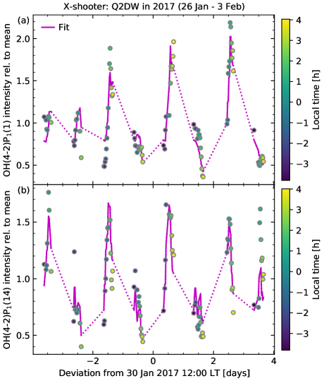
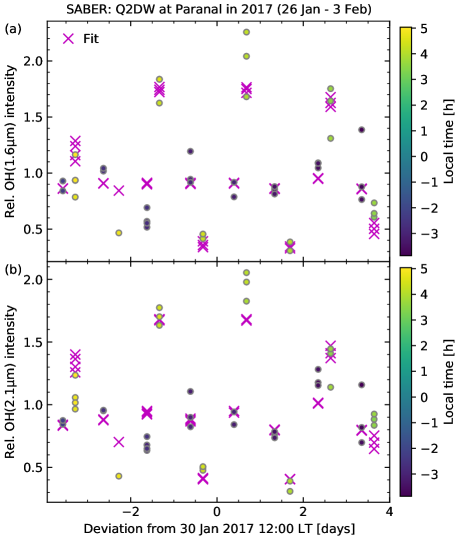
In this section, we discuss the results of the Q2DW fits of the X-shooter-based OH line measurements for the wave event in 2017. Figure 1 shows examples of the corresponding time series of 30 min bins (section 2.1) for the doublets OH(4-2)P1(1) (a) and OH(4-2)P1(14) (b), which only differ by the rotational quantum number. However, the difference in the rotational energy of 3,239 cm-1 is the largest of the entire set of 298 lines. Hence, the variability patterns should deviate. The inspection of the figure confirms this assumption. Deviations can be observed in the day-to-day development of the maximimum and minimum relative intensities and the local times showing these extreme values. Nevertheless, the basic pattern is similar. There are alternating nights with low and high relative intensities, which clearly points to the presence of a Q2DW. The apparent amplitudes are large. For OH(4-2)P1(1), the maximum-to-minimum ratio is 6.1. The standard deviation relative to the mean for the 88 bins indicates 0.45. For OH(4-2)P1(14), the corresponding values for the 86 available bins are slightly lower (4.4 and 0.36, respectively).
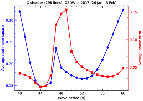
Figure 1 also displays our best fits with LT-dependent amplitudes for both OH emissions. The fits were performed for all LT bins except for 04:00 to 05:00, which includes only a single observation (Table 1). The fixed period for all LT bins was set to 44 h. This decision is justified by Figure 2, which shows the root mean square (rms) for the differences between fit and observed data relative to the line-specific mean intensity averaged for all 298 lines as a function of the period grid from 40 to 60 h. Moreover, the average phase error relative to the period (Table 1) is displayed for the same set of lines and periods. The minimum values of both indicators (0.15 for the rms and 0.015 for the phase uncertainty) are clearly located at 44 h. The accuracy of this period, which is limited by the step size of 1 h, is highly sufficient for the estimation of emission heights as we will discuss in section 4.3. Moreover, note that the scatter in the periods from the minimum rms derived for the individual lines is fairly small (63% with 44 h and 33% with 45 h) despite significant differences in the time series. Q2DW periods below 48 h appear to be rather typical in regions close to Cerro Paranal as long-term OH observations at El Leoncito (31.8∘ S, 69.3∘ W) indicate [Reisin (\APACyear2021)]. Figure 2 reveals that periods close to 2 full days are not able to reproduce the change of the variability pattern from night to night shown in Figure 1. In particular, the small apparent amplitudes of the first two nights for OH(4-2)P1(1) suggest that the maximum and minimum were outside the range of local times covered by the X-shooter data, i.e. too late in the morning. With a period distinctly smaller than 48 h, it was then possible to observe the extreme intensities afterwards at nighttime. Therefore, the time series is just long enough to robustly derive a wave period. The variability pattern of OH(4-2)P1(14) is more regular at the beginning with high deviations from the mean intensity, which excludes that the Q2DW was significantly weaker in the first nights as the consideration of only the P1(1) data could suggest. The differences between both lines are obviously the result of shifts in the positions of the extremes. Consequently, both emissions need to show different Q2DW phases. Our fits revealed phases of 0.403 and 0.229 at the reference time for the lines with and 14, respectively. The resulting phase difference is much larger than the mean uncertainty reported above (which should be even smaller for phase comparisons). Hence, the wave of 2017 is obviously suitable to safely separate lines based on their fitted phases.
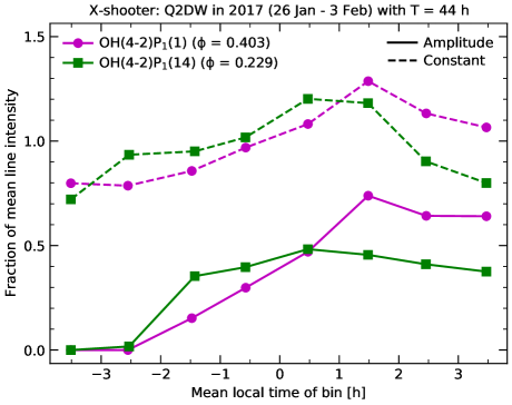
The results for the two example doublets are further analyzed in Figure 3, which shows the amplitude, i.e. the product of the fit parameters and relative to the mean intensity of the time series, as a function of the mean local time for intervals with a width of 1 h. The wave amplitudes of both emissions strongly depend on local time. There is no detection of a Q2DW before 22:00. Afterwards the amplitudes increase and then become relatively stable. This development is faster for OH(4-2)P1(14), where a shallow maximum with an amplitude of 0.46 is visible between 0:00 and 01:00. The maximum for OH(4-2)P1(1) is significantly higher and amounts to 0.74. It is present between 01:00 and 02:00. These remarkable structures cannot be explained by a single wave with fixed amplitude. A model with multiple wave components would certainly better reproduce the patterns, but at least a model with two components did not return reliable wave properties (section 3). The persistent lack of wave-like variability at the beginning of the nights is hard to explain in this way. Hence, our assumption of LT-dependent Q2DW amplitudes, which leads to the narrow peaks of the fit models in Figure 1, appears to be the most promising approach for achieving a satisfying agreement with the observed time series. This model requires that the physical conditions that control the wave propagation and/or the sensitivity of the OH emission for Q2DWs change depending on the time of the day. Nonlinear interaction with especially the diurnal and semidiurnal tides [<]e.g.,¿palo99 could explain this behavior. In this context, phase locking, which would significantly weaken the diurnal tide [Walterscheid \BBA Vincent (\APACyear1996), Hecht \BOthers. (\APACyear2010), Walterscheid \BOthers. (\APACyear2015)], did not seem to be active at Cerro Paranal during the considered time interval as periods very close to 48 h cannot explain the time series. The LT dependence of the Q2DW amplitude in OH emission might also be affected by the negative nocturnal trend of atomic oxygen (produced at daytime) that would always be present without vertical dynamics especially at the lowest OH emission altitudes [Marsh \BOthers. (\APACyear2006)].
Figure 3 also shows the constant (or factor) relative to the mean intensity. For an undisturbed cosine oscillation centered on the mean intensity of the time series, should be close to 1 (see section 3). In reality, the values range between 0.7 and 1.3. They cause that the maximum are not located at the end of the night as in the case of (not shown). Although the joint fitting of and might lead to some systematics due to possible degeneracies, asymmetries in very large intensity variations that cause larger deviations during the crest of the wave are more likely. Moreover, there are also variations in the nocturnal OH intensity without a wave. An inspection of the entire X-shooter data set suggests that this is probably a minor effect as the climatological changes for the investigated times in southern summer are of the order of only 10% [<]cf.¿noll17. The intensity even tends to decrease with increasing LT in contrast to our results for .
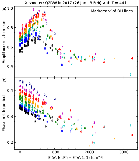
Next, we discuss the whole set of 298 lines. Figure 4a shows the line-specific maximum of the amplitude of all hour intervals as a function of the energy of the upper state of the transition relative to the lowest energy of the corresponding vibrational level . The reference states are characterized by a rotational quantum number and the electronic substate () [<]e.g.,¿noll20, i.e. the energy difference equals 0 cm-1 for P and Q lines. If we focus on these lines, the figure reveals a clear increase of the amplitude for decreasing with values between 0.56 for and 0.74 for . This trend is highly significant as the uncertainties derived from lines with the same upper level are only about 0.02. The amplitude differences for adjacent vibrational levels are larger for high . For increasing rotational energy, we find an increase for all vibrational levels which is more pronounced for low . Up to about 500 cm-1, the increase ranges from 0.12 for to 0.23 for . For the lowest vibrational levels, this rise results in enormous amplitudes of more than 90% of the sample mean intensity. At higher rotational energies, the amplitudes decrease again. This trend appears to start slightly later for lower , but not later than about 700 cm-1. The drop of the amplitude is much stronger for lower . For the highest , the amplitude appears to be independent of the vibrational level and is distinctly smaller than for low . The mean amounts to about 0.48 for energy differences larger than 1300 cm-1.
The complex pattern in Figure 4a needs an explanation. As we can expect that the emission altitudes increase with higher and [<]e.g.,¿adler97,dodd94,noll18b,savigny12, lower amplitudes with increasing quantum numbers imply a decrease of the wave amplitude with increasing altitude. Such a trend is consistent with the dependence of the amplitude on for up to at least 1,000 cm-1 and the comparison of amplitudes for very low and very high . An issue seems to be that the highest amplitudes are located at intermediate rotational energies. However, this feature can be explained by means of the structure of the OH rotational level population, which can be characterized by a cold and a hot population for each [Cosby \BBA Slanger (\APACyear2007), Kalogerakis \BOthers. (\APACyear2018), Kalogerakis (\APACyear2019), Noll \BOthers. (\APACyear2020), Oliva \BOthers. (\APACyear2015)]. While the temperature of the cold population, which dominates the emission at low , is consistent with the ambient temperature, i.e. about 190 K on average at Cerro Paranal [Noll \BOthers. (\APACyear2016), Noll \BOthers. (\APACyear2020)], the hot population shows apparent temperatures between about 700 K for [Noll \BOthers. (\APACyear2020)] and about 12,000 K for [Oliva \BOthers. (\APACyear2015)]. Such extreme values reflect significant deviations from the local thermodynamic equilibrium (LTE), which are related to the non-LTE nascent population of the hydrogen–ozone reaction [Llewellyn \BBA Long (\APACyear1978)] as well as an insufficient frequency of collisions that thermalize the rotational level population compared to -changing collisions and the radiation of airglow photons [Noll \BOthers. (\APACyear2018)]. An inspection of the combined populations now shows that the contributions of the cold and the hot component are of the same order at similar as those where we find the maximum amplitudes in Figure 4a [Noll \BOthers. (\APACyear2020)]. Consequently, the latter can be explained by an increased sensitivity of the corresponding OH lines to the Q2DW due to the strong impact of the wave-induced variation of the ambient temperature (affecting the cold population) on the rotational energy where cold and hot populations have similar contributions. Changes in the cold component are more crucial because of its much steeper decline with increasing energy. Also note that the relative contribution of the hot population is lower than a percent for at 0 cm-1 [Noll \BOthers. (\APACyear2020), Oliva \BOthers. (\APACyear2015)]. The rapid growth of this fraction with increasing can then explain the increase of the Q2DW amplitudes until the maximum values at 500 to 700 cm-1. Moreover, the drop of the amplitudes marks the energies where the contribution of the cold population becomes minor. Hence, the highest show a pure hot population, which can obviously be described by a single amplitude. The lack of a dependence of the amplitude on suggests that the -specific hot components are linked and might be represented by a single population (at least in part). The structure of the full roto-vibrational populations, which show connections between high for adjacent [Cosby \BBA Slanger (\APACyear2007), Noll \BOthers. (\APACyear2020)], seems to confirm this interpretation.
Q2DW phases relative to the period of 44 h at 30 January 2017 12:00 LT are shown for all 298 OH doublets in Figure 4b. In general, there is a clear decrease of the phase with increasing and . For the levels with and , the phase ranges from 0.436 for to 0.333 for , which is distinctly more than the uncertainty of 0.005 derived from lines with the same upper levels. For higher , the phases decrease almost linearly and similar for all with shifts of about 0.04 up to about 500 cm-1. The trend may even hold until about 1,500 cm-1 but with a decreasing difference between low and high . For the highest , there is a flattening of the phase change, which might even stop at the end. However, this remains questionable due to the relatively small number of lines and relatively high uncertainties. The average phase for cm-1 is 0.23, which is about 0.2, i.e. almost 9 h, lower than the maximum shown by OH(2-0)P1(1). This relatively large spread is promising in terms of a sensitive derivation of effective emission heights for various OH emission lines (see section 4.3).
4.2 OH Emission Profiles
In order to link wave phases and heights, we need altitude-resolved OH emission measurements. The required data were obtained by the two OH channels of the limb-scanning SABER radiometer (section 2.2). For a comparison with the X-shooter-based time series, Figure 5 shows vertically integrated VERs of the channels OH(1.6 m) (a) and OH(2.1 m) (b) relative to the mean of the 44 measurements that are representative of the region around Cerro Paranal during the eight nights in 2017 covered by the X-shooter data set. Both channels show variability patterns that are consistent with a strong Q2DW for the 22 data points taken at about 04:00 LT, whereas the data related to about 21:00 LT do not display clear wave features. These results agree with those of the X-shooter data set in terms of the pronounced time dependence of the wave amplitude (Figure 3). The maximum-to-minimun ratios and standard deviations relative to the mean are 7.4 and 0.46 for all OH(1.6 m) data and 6.6 and 0.42 for all OH(2.1 m) data. The smaller values for the latter are consistent with the decrease of the wave amplitude with increasing for the X-shooter data (Figure 4). Remember that the effective are about 4.6 and 8.3 for the two SABER OH channels (section 2.2). The maximum-to-minimum ratios are higher than the values of 6.1 for OH(4-2)P1(1) and especially 4.4 for OH(4-2)P1(14) (section 4.1). The standard deviations are very similar to the value of 0.45 for the line with but higher than the result of 0.36 for the line with high . These findings agree well as the integrated emission of the SABER channels is dominated by lines with small . Consequently, SABER and X-shooter data show a consistent picture of the Q2DW event in 2017. Differences in the measurement approaches and sample properties do not appear to have a significant impact.
Figure 5 also shows our fits of the two LT ranges based on the approach described in section 3. Compared to the 04:00 LT data that we exclusively used for the phase derivation, the amplitude for the 21:00 LT data was significantly smaller. The ratios for the 21:00 and 04:00 amplitudes were about 0.09 for OH(1.6 m) and about 0.20 for OH(2.1 m). Thus, the fit of the evening measurements shows only very small Q2DW-related variations. Moreover, the corresponding factors for were 0.86 and 0.87, i.e. the intensity level for the evening data was lower on average. For the subsequent analysis, we only focused on the morning data.
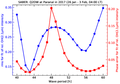
The fitting was performed for the same wave period as in the case of the X-shooter data, i.e. 44 h (section 4.1). Using the same period is important for the derivation of the effective emission heights. Nevertheless, we checked a wide range of periods in terms of the fit quality. The results for OH(2.1 m) and the 04:00 LT data are shown in Figure 6. The corresponding plot for OH(1.6 m) is very similar. The rms relative to the mean indicates a clear minimum of 0.13 at 43 h. The phase error derived from the fit also shows a minimum there (0.013), although it is less pronounced. Consequently, the SABER-related fit returns the best result for a period which is only 1 h lower than for the X-shooter data. This shift can also be observed for the maximum phase uncertainty (48 vs. 49 h). In the view of the various differences between both data sets, the deviation is small. It is not crucial for the estimates of the line-specific emission altitudes. A comparison of the results for 43 and 44 h did not indicate significant deviations with respect to the general uncertainties (section 4.3). In the following, we will focus on the results for 44 h, which represents the best period from the X-shooter data set, which is much larger than the SABER data set in terms of OH emission features and observing times.
Interestingly, the period can change significantly if the geographical area is not restricted to locations close to Cerro Paranal. Our additional check of the SABER data without longitude and LT limits (cf. section 3) revealed a most likely period of 49 h for the two OH channels. This result is in good agreement with the findings of \citeAgu19, who reported a period of 48 h for the Q2DW in 2017 based on the kinetic temperatures from SABER. We repeated this fit and found the same. For the global fits, we preferentially used the combined evening and morning data, i.e. we neglected a possible LT dependence of the amplitude. This setting resulted in better fits, which is also in contrast to our experience with the data restricted to the region around Cerro Paranal. Moreover, an inspection of the wave properties depending on the longitude showed that the South American sector exhibited the clearest Q2DW variability pattern. In other regions, the wave was much less pronounced. This observation may explain why \citeAgu19 only identified an intermediate wave amplitude of 10 K at 82.5 km for the event in 2017. The latitude- and time-resolved SABER-based results for a fixed period of 48 h from \citeAxiong18 show amplitudes slightly below 10 K at 84 km at about 25∘ S for the relevant time interval at the end of January and beginning of February. We find about 18 K around Cerro Paranal in the morning. In addition, the local times with the strongest variations changed depending on longitude, which indicates why global fits without the corresponding scaling factors worked better. This complex variability pattern suggests that the Q2DW is significantly disturbed by interactions with other planetary waves, tides, gravity waves, and/or the mean flow. For OH emission from SABER observations, \citeApedatella12 already found a complex longitude dependence of the Q2DW-related variability due to contributions of nonmigrating tides, stationary planetary waves, and secondary waves that are preferentially generated by the nonlinear interaction of the Q2DW and migrating tides. The latter supports our assumption that such interactions were important for the Q2DW event in 2017 with a pronounced LT dependence of the measured amplitude.
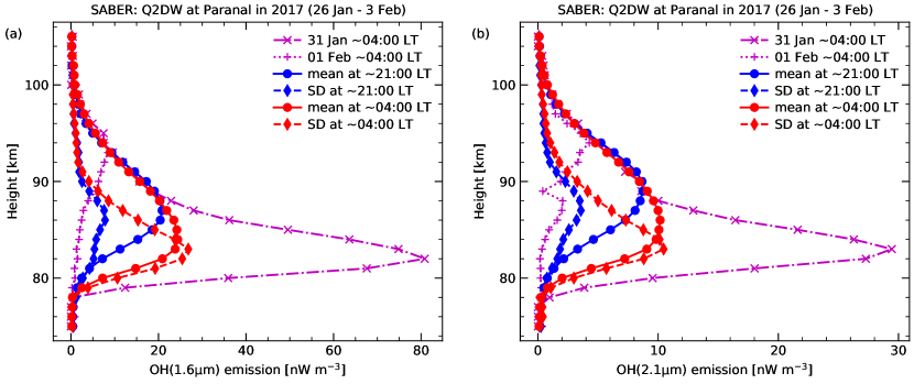
We now turn to the discussion of the height-dependent impact of the Q2DW. Figure 7 shows different kinds of emission profiles for the two OH channels centered on 1.6 m (a) and 2.1 m (b). For each channel, two individual profiles from 31 January and 1 February 2017 at about 21:00 LT are displayed. The huge differences between both profiles with a time difference of 1 day demonstrate the implications for the OH emission by a large amplitude Q2DW. On 31 January, the OH(1.6 m) profile peaked at a very low altitude of 82 km with an enormous VER of 81 nW m-3. In contrast, the emission almost vanished completely at this altitude on the next day. As only the emission at the highest altitudes remained relatively similar, the peak moved upward by 11 km to 93 km, where the VER was only 8 nW m-3. The situation for OH(2.1 m) is very similar with the peaks just 1 km higher. It is not clear whether the VER minimum at 89 km on 1 February is real as it cannot be seen in the corresponding data from OH(1.6 m).
Figure 7 also shows mean and standard deviation profiles for the two LT regimes of about 21:00 and 04:00 in the eight selected nights. The evening data indicate typical mean profiles with respect to the long-term averages for Cerro Paranal [Noll \BOthers. (\APACyear2017)]. The centroid altitudes of the plotted profiles of both channels are 88.1 and 89.5 km, respectively. The standard deviation profiles of the 21:00 LT data only indicate relatively weak variations. The peaks of these profiles are about 1 to 2 km lower than for the mean profiles. These shifts are expected due to the steepening of the atomic oxygen gradient with decreasing height [<]e.g.,¿smith10, which makes the lower altitudes more sensitive to vertical transport of this important gas for the OH production and subsequent relaxation and destruction processes. The strong oxygen-induced emission variations at low altitudes lead to a significant perturbation of the mean profile for the morning data. The latter therefore extends to lower heights (with a 3 km lower peak) and gets more broadened for both channels. The peak of the standard deviation profile moves in a similar way. The emission variability is much larger than in the case of the evening data (as expected). Note that the mean centroid emission altitudes of the individual profiles for 04:00 LT of 88.1 km for OH(1.6 m) and 89.1 km for OH(2.1 m) are very similar to those of the 21:00 LT data (88.0 km and 89.5 km) since the large differences in the VERs which affect the plotted mean profiles do not matter here. Nevertheless, the larger impact of the Q2DW on the morning data can be recognized by the standard deviation of the individual centroid altitudes of about 2.3 km for both OH channels, which is distinctly higher than about 0.6 km for the evening data (if one outlier is excluded).
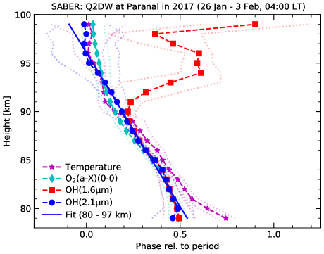
With the knowledge of the height-dependent response of the OH emission on the passing Q2DW, we now discuss the wave phases as a function of altitude. Figure 8 shows the phase functions between 79 and 99 km from fits of the morning data with a period of 44 h as described in section 3 for both OH channels. The phases are given for 30 January 2017 12:00 LT at Cerro Paranal. At least for the altitude range between 80 and 90 km, there is a clear trend of decreasing phase with increasing height for the OH emissions at about 1.6 and 2.1 m. For 80 to 89 km, both curves are almost identical with a mean absolute difference of only 0.005. However, the discrepancy is rapidly growing above 89 km. While the trend continues for OH(2.1 m), OH(1.6 m) shows a complex behavior with increasing and decreasing phase. The latter is not trustworthy. As expected from the ratio of standard deviation to mean profiles in Figure 7, the fitted wave amplitudes relative to the mean rapidly decrease with increasing altitude. From 80 to 93 km, drops from 1.18 to 0.19 for OH(2.1 m). However, this is still moderate compared to a decrease from 1.23 to 0.04 for OH(1.6 m). Consequently, it appears that the wave-induced variability in the emission at about 1.6 m was too low to track the wave in a reliable way (cf. evening data in Table 1 and Figure 3), whereas it was still sufficient for OH(2.1 m). Note that the latter emission peaks higher in the atmosphere (Figure 7).
In order to check this interpretation, we also fitted the emission of O2(a-X)(0-0) at about 1.27 m, which is also observed by SABER. The profile of this airglow emission strongly changes during the night [Noll \BOthers. (\APACyear2016)] due to the decay of an excited population originating from ozone photolysis at daytime [<]e.g.,¿lopez89. However, in the second half of the night, the emission distribution is similar to the one of OH. The fits only show a relatively weak decrease of the wave amplitude by a factor 2 over the entire plotted altitude range. Hence, the resulting phases in Figure 8 appear to be reliable. They clearly support the trend found for OH(2.1 m). This result is further confirmed by fits of SABER-based kinetic temperature profiles [Dawkins \BOthers. (\APACyear2018)], where the corresponding phase profile is also plotted. The temperature fits are relatively robust since the wave amplitude remained relatively high in the entire studied altitude regime (at least 11 K up to 98 km with maximum values of about 18 K at 82 km and 21 K at 94 km). The shape of the atomic oxygen profile does not matter for the temperature.
In conclusion, we have strong hints for a monotonically decreasing phase with increasing height over the entire altitude range relevant for OH. This implication is ideal for the estimate of effective emission heights. Moreover, the earlier maxima at higher altitudes indicate that the wave was rising. This interpretation is also supported by test fits of the diurnal tide with the same fitting algorithm [<]cf., e.g.,¿griffith21. Consequently, the wave propagation is consistent with the assumed origin of Q2DWs in the lower mesosphere [<]e.g.,¿ern13. The results suggest that the OH-relevant wave phases are best described by the profile fits for OH(2.1 m). There is an almost linear relation between phase and height over a wide altitude range. We found that the optimimum interval for a linear regression extends from 80 to 97 km. Then, we obtain a very high coefficent of determination r2 of 0.995. The inverse slope of the regression line corresponds to the vertical wavelength of the wave. It amounts to km, which is near the peak of the distribution of W3 Q2DW wavelengths derived by \citeAhuang13 based on SABER data. If we only consider the altitude range up to 89 km, where OH(1.6 m) can also be used, it is almost the same but with a larger uncertainty ( km). For OH(1.6 m), we then obtain km, which agrees within the regression uncertainties.
4.3 Effective OH Emission Heights
Combining the line-specific effective phases from section 4.1 with the slope of the relation between phase and height for OH(2.1 m) from section 4.2 for the same wave period of 44 h allowed us to estimate the effective emission heights of 298 OH lines. For a direct conversion, it is just necessary to subtract the phase for each line from the intercept at 0 km of 3.027 and to multiply the result with the vertical wavelength of 31.74 km (see section 4.2). However, our calculation was more complex as we also considered possible phase deviations due to the differences in the lines of sight as well as geographical and temporal distributions of the X-shooter and SABER measurements for the Q2DW event in 2017. In order to estimate this effect, we used the fitted effective phases of 0.388 and 0.345 for the vertically integrated VERs of the OH channels centered on 1.6 and 2.1 m, respectively, and compared them with X-shooter-based effective phases for sets of OH lines that are representative of these channels. We weighted the phases for individual lines as shown in Figure 4b by the product of the measured line intensity and the channel-specific transmission [Baker \BOthers. (\APACyear2007)] at the line position. Moreover, we checked the impact of the fact that our line sample is not complete (section 2.1). We found that the effective of our line mixes did not change for OH(1.6 m) but deviated by for OH(2.1 m) compared to the reference values of 4.57 and 8.29 by \citeAnoll16. However, lowering the contribution of the lines to get a match in the effective for OH(2.1 m), i.e. 8.29, did not affect the effective phases, which turned out to be 0.379 and 0.327 for the X-shooter data. Consequently, the SABER phases appear to be shifted by about 0.0135 on average. We subtracted this value from the intercept of the regression line before we calculated the effective emission heights. In terms of altitude, this shift corresponds to a change of km with an uncertainty of 0.13 km derived from the difference between the results for both channels.
For the estimate of the height uncertainties, we also checked whether our simple linear regression analysis without the consideration of the height-dependent fit quality (Figure 8) could cause systematic phase offsets. For this purpose, we calculated a residual phase deviation from the differences between measured phase and regression line at all heights weighted by the wave-induced variability. The resulting height uncertainty only amounts to 0.11 km thanks to the convincing fit of the OH(2.1 m) profile data. Concerning the X-shooter-related uncertainties, we used the representative phase uncertainties 0.005, 0.008, and 0.017 (cf. caption of Figure 4), which are based on phase differences for OH lines with the same upper level for the energy differences below 400 cm-1, between 400 and 800 cm-1, and above 800 cm-1, respectively. Combined with the small uncertainties reported above, the effective absolute height errors resulted in about 0.24, 0.30, and 0.55 km, respectively.
The effective heights for the 298 OH doublets range from 81.8 to 89.7 km with an average of 84.88 km and a standard deviation of 1.43 km. Compared to the uncertainties, the line-specific differences are highly significant. The given altitudes are representative of the maximum emission variability induced by the Q2DW in the eight investigated nights of 2017. This can be illustrated for the vertically integrated VERs of the SABER channels at 1.6 and 2.1 m, for which we derived effective heights of 83.75 and 85.13 km based on the already stated phases. The profile plots for about 04:00 LT in Figure 7 indicate that these wave-related heights are between the peak at 83 km and the centroid altitude at 84.6 and 85.6 km of the standard deviation profiles of the two channels.
If the evening data of both instruments had resulted in reliable wave fits, we would probably have obtained significantly higher altitudes in agreement with the standard deviation profiles of these data. Hence, the resulting heights of our approach depend on the wave properties and the state of the background atmosphere during the analyzed time interval. Therefore, it is desirable to also provide heights for the studied OH lines which are representative of longer time scales. Moreover, there should be a closer relation to the peak or centroid emission altitudes that are usually used in the literature, especially with respect to studies of OH rotational temperatures as indicators of the effective ambient temperature for the OH emission layer. The relevant heights for temperature and intensity variations can differ by several kilometers [<]e.g.,¿swenson98. For example, we find for the ratio of the intensities of OH(3-1)P1(1) and OH(3-1)P2(2), which are often used for rotational temperature studies [<]e.g.,¿beig03,schmidt13,noll15, a phase shift of compared to the mean phase for both lines that corresponds to an altitude difference of km with an uncertainty of several hundred meters (including a possible small discrepancy in the phase–height relations of temperature and OH intensity as indicated by Figure 8). Note that the general use of temperatures instead of intensities for height estimates is not possible as rotational temperatures show much higher measurement uncertainties and could vary in a different way than the satellite-based kinetic temperatures due to the non-LTE contributions which increase with increasing and [Noll \BOthers. (\APACyear2020)]. For the derivation of the reference heights, we considered the 14-year averages of the centroid altitudes of km for OH(1.6 m) and km for OH(2.1 m) from \citeAnoll17 that were calculated based on 4,496 SABER profiles taken close to Cerro Paranal. These values are about 4.06 and 4.07 km higher than our results for the Q2DW phase fits but they are close to the averages of the individual centroid altitudes during the investigated event (section 4.2). The large difference can therefore be mainly explained by the strongly increasing VERs for emission profiles with lower peaks and the resulting impact on the vertical variability distribution. It is promising that the shifts are almost the same for both OH channels as it implies that the Q2DW-based effective height differences between lines are also representative of the long-term averages of the centroid emission heights. At least for lines with low that mainly contribute to the SABER VERs, the deviations should be much smaller than the stated uncertainties of a few hundred meters. Consequently, we can also provide effective OH emission heights for average conditions at Cerro Paranal by shifting all line-specific heights by km. The resulting mean height for all 298 doublets is 88.95 km, which is in between the centroid altitudes for the reference profiles of both SABER OH channels.
Our height estimates are based on a model that assumes a single wave with a period of 44 h and an amplitude depending on local time. In order to increase the confidence in the corresponding results, it is important to know how changes in this model affect the derived emission heights. As already mentioned in section 4.2, we could have also used a period of 43 h as indicated by the SABER-based fit results in Figure 6. In comparison to 44 h, we obtained a mean height for the 298 lines which is 0.09 km higher before and 0.02 km lower after the shift. The standard deviation did not change, i.e. it is 1.43 km. Hence, the impact of a period change by 1 h is negligible. We also performed a test for an extremely different period of 56 h, which marks a secondary minimum of the phase error in Figure 6 and results in a downward-propagating Q2DW with a of km for OH(2.1 m). Nevertheless, the changes of the two mean heights were only and km and the standard deviation just decreased by km. This promising result demonstrates that even an unrealistic period can lead to reliable heights as long as a sufficiently linear phase–height relation with a significant spread of phases is present. For this reason, periods around 50 h do not work for the analyzed Q2DW as they mark the reversal of the vertical propagation direction, which leads to very long . In section 3, we have already discussed a two-wave model with fixed amplitudes that we checked as an alternative but resulted in unlikely wave parameters and low-quality fits. Nevertheless, even such a model appears to provide useful information on the OH height distribution. Focusing on the standard deviation of the effective heights of all lines, the best-fitting waves with periods of 43 and 51 h and opposite vertical propagation directions returned 2.18 and 0.72 km. Both values show a large discrepancy but the average is 1.45 km, which is very close to the value for our preferred model of 1.43 km.
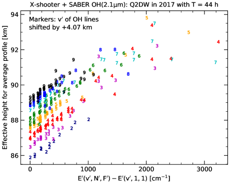
With the confirmation of the robustness of our results, we now show the distribution of the reference heights for all investigated OH lines in Figure 9. The altitudes range from 85.9 to 93.8 km, i.e. the maximum difference is almost 8 km and therefore of the same order as the width of the full OH emission layer [<]e.g.,¿baker88. The detailed structure of the plotted data distribution was already discussed in terms of the wave phases in section 2.1. The distribution is just inverted compared to the phases in Figure 4b. The effective emission heights increase for higher vibrational and rotational excitations as expected. Focusing on the levels with and , the altitude difference between (89.14 km) and 2 (85.89 km) amounts to 3.26 km, which is about 0.47 km for a difference of 1 in on average. This result agrees very well with the corresponding values found in previous studies of a few OH bands related to satellite data [Noll \BOthers. (\APACyear2016), Sheese \BOthers. (\APACyear2014), von Savigny \BBA Lednyts’kyy (\APACyear2013), von Savigny \BOthers. (\APACyear2012)] and ground-based data combined with a sodium lidar [Schmidt \BOthers. (\APACyear2018)]. The height difference for decreases with increasing vibrational excitation. Our analysis revealed 0.59 km for but 0.29 km (i.e. the half) for . This behavior agrees qualitatively with the modeling results of \citeAsavigny12 and is obviously caused by the -dependent Einstein and collisional rate coefficients. As the previously published results refer to emissions of bands instead of lines, we also checked the change of the height differences with increasing rotational energy. Taking only data with between 400 and 600 cm-1 ( between 4 and 6) as in section 4.1, we found almost the same difference between and 2 (3.20 km) but at altitudes that are about 1.1 km higher. The change of the differences for with also agrees within the uncertainties. Consequently, the results for entire bands should agree with those of the significantly contributing brighter lines of low to intermediate .
For the highest rotational levels, we do not see a clear dependence of the effective emission altitudes on . The differences appear to decrease with increasing . As the nearly linear height increase with seems to flatten (especially for higher ), there might even be a nearly constant effective emission height for the highest . This behavior was already modeled by \citeAdodd94. However, quantitatively, there are some discrepancies. Our mean for all lines with cm-1 is 92.3 km. If we assume that this height is representative of all , we estimate -specific maximum changes compared to cm-1 between 3.2 and 6.4 km. \citeAdodd94 only modeled 0 to 2 km and a reference height for the highest of 89 km. Based on the data set of \citeAnoll17 that we also used for the derivation of our reference heights, \citeAnoll18b modeled rotational level populations with a focus on . For two models with very different rate coefficients for collisions of OH with atomic oxygen, the maximum height changes resulted in 1.5 and 2.8 km and a maximum emission height of almost 92 km in the latter case. If we estimate the height changes from the plotted data for , we obtain a rough lower limit of 1.5 to 2 km. These values might be better for a comparison since levels with cm-1 would be far beyond the exothermicity limit of the hydrogen–ozone reaction [Cosby \BBA Slanger (\APACyear2007), Noll \BOthers. (\APACyear2018)] of about 1,070 cm-1. In any case, the model results appear to match the correct order of magnitude, although the uncertainties are large. The model of \citeAnoll18b also predicts a flattening of the height increase for high . Moreover, this model gives nearly constant heights for the lowest . The latter is something which we do not find in our analysis that suggests a linear increase due to the growing contribution of the hot population. The nearly constant height for the OH lines with the highest of all also seems to be supported by the measured wave amplitudes. The interesting levels are occupied by a pure hot population [Noll \BOthers. (\APACyear2020)], which appears to show a nearly constant amplitude for the Q2DW in 2017 (Figure 4). Moreover, the SABER-based fits of the profiles indicate a steep gradient of the amplitude at the heights relevant for OH (section 4.2). Hence, an almost constant amplitude would require a relatively narrow altitude distribution for the OH lines dominated by the hot population. For lower , the interpretation of the wave amplitudes is more difficult due to the mixing of cold and hot populations with different altitude distributions.
4.4 Impact of Time Range
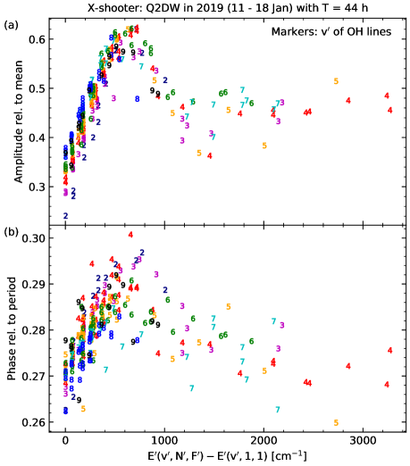
Our OH height estimates are based on eight nights of a single Q2DW. Although they appear to be reliable according to the discussion in section 4.3, the analysis of another wave event would be a good quality check. As already described in section 2.1, we were able to identify another Q2DW in the X-shooter data of seven nights from 11 to 18 January 2019. We analyzed the corresponding line measurements in the same way as for the Q2DW in 2017. However, we only considered lines with wavelengths shorter than 2.1 m because of too few spectra taken without a -blocking filter (section 2.1). The resulting fits showed that a period of 44 h also appears to be the best choice. On the other hand, the LT dependence of the wave amplitude was very different from the curves in Figure 3. The variation was much smaller. The maximum and minimum values only differed by a factor of 2 for the two example lines. Moreover, the highest amplitudes were reached between 22:00 and midnight, which corresponds to a shift of h compared to the data from 2017. While the maximum relative amplitude for OH(4-2)P1(14) did not change much (0.49 vs. 0.46 for 2017), it was significantly lower for OH(4-2)P1(1) (0.31 vs. 0.74 for 2017). As a consequence, hot populations obviously showed a stronger response to the Q2DW than cold populations, which is the opposite situation compared to 2017. This reversal was also seen for the dependence of the amplitude on for low (Figure 10a). Nevertheless, the impact of the mixing of both populations at intermediate rotational energies (400 to 800 cm-1) was similar. The related lines showed the largest amplitudes, although only values up to about 0.62 were found. In conclusion, the two-population model appears to be confirmed by the data from 2019. However, the Q2DW was weaker and showed different amplitude relations, which suggests that the properties of such waves are highly variable due to changes in their generation, propagation, and interaction with the background atmosphere (including other waves). This high amount of variability had already been observed before [<]e.g.,¿ern13,gu19,tunbridge11.
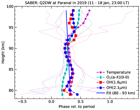
For our purpose, it is important that a wave can be used for estimates of effective emission heights. Hence, the phase relations are crucial. Unfortunately, the pattern for our set of OH lines was completely different from the situation in 2017 (Figure 4b). A clear dependence was not found and there was no monotonic decrease of the phase with increasing (Figure 10b). Instead, the phase even increased up to about 600 cm-1. The expected behavior was only present for higher energies. An important detail for the explanation of this unexpected structure is the maximum range of phases, which amounts to only 0.041. The standard deviation was 0.007. Consequently, the phase was almost constant. We also fitted the available SABER data for a better understanding. For the seven nights in 2019, we could use 19 profiles, all taken at about 23:00 LT (section 2.2). The profile fits for both OH channels agree quite well with the X-shooter data. There were only small phase changes without clear direction (Figure 11). For OH(2.1 m), we found a maximum phase difference of only 0.13 for the height interval between 80 and 93 km, which minimizes the deviation of the fitted phases from a linear relation. The resulting regression line is almost vertical with a highly uncertain wavelength of km. The rising wave turns into a descending one with km for a fit up to 97 km as in the case of 2017 (Figure 8). Hence, the propagation direction remains unclear. The long wavelength may explain the reduced dependence of the wave amplitude on the OH line parameters (partly related to the emission height) and local time. The latter might point to a less efficient interaction of the Q2DW with the migrating diurnal tide, which has a relatively short [<]e.g.,¿forbes95 that is similar to the about 32 km for our best fit of the Q2DW in 2017.
huang13 investigated of southern W3 Q2DWs based on SABER temperature data from 2002 to 2011 and found a wide range of possible values from above 10 km to beyond 100 km at an altitude of 85 km. As other studies using different techniques also found a high variability for low-to-middle southern latitudes in the mesopause region [Ern \BOthers. (\APACyear2013), Guharay \BOthers. (\APACyear2013), Reisin (\APACyear2021)], the differences in for the analyzed Q2DWs in 2017 and 2019 do not appear to be uncommon. For a strong event in southern summer 2002 to 2003, \citeAhuang13 also investigated the change of the wavelength over the lifetime of the wave of several weeks. They found a trend of decreasing and less variability with increasing age. As we investigated data from 11 to 18 January in 2019 but from 26 January to 3 February in 2017, this trend would be consistent with our wave fits. However, as the Q2DWs can be quite different from year to year, a convincing check would need a detailed wave analysis over the entire lifetime for the different years. In any case, the properties of the Q2DW in the selected time interval in 2019 were not suitable for our phase-sensitive investigation.
5 Conclusions
In our study, we derived reference centroid emission heights for average conditions of various individual OH lines for the first time. This success required the combination of OH line intensities from ground-based spectra taken with the astronomical X-shooter spectrograph at Cerro Paranal in Chile and space-based limb sounding of emission profiles in the two OH-related channels of the SABER radiometer on TIMED. Moreover, we benefited from the observation of a strong quasi-2-day wave (Q2DW) with both instruments in eight nights at the beginning of 2017. For the region around Cerro Paranal and the given observing period (mainly limited by the X-shooter data coverage), our wave fits of both data sets (separated depending on local time) with a cosine function revealed a most likely period of 44 h and vertical wavelength of about 32 km (based on the SABER channel centered on 2.1 m), which makes this wave event very suitable for phase-sensitive investigations. The amplitudes strongly varied. Our fits revealed particularly high amplitudes up to almost 100% of the mean intensity for emission lines related to intermediate rotational energy between 400 and 800 cm-1 and low vibrational upper level , the second half of the night, and altitudes below the emission peak. The high values for lines with intermediate rotational energies indicate an amplification of the variation due to the mixing of cold (thermalized) and hot (non-thermalized) OH rotational level populations, which maximizes for the stated energy range. The local time dependence (with no wave detection at the beginning of the night) suggests that the Q2DW was strongly affected by the changing diurnal atmospheric conditions (e.g. by tides). Apart from the altitude dependence of the intrinsic amplitude of the upward-propagating wave, the OH emission should also be affected by the increasing relative atomic oxygen variability with decreasing height. Furthermore, the wave properties significantly depend on the selection of the geographical area and the time range. Another Q2DW which was present in the X-shooter data of 2019 indicated a vertical wavelength being too long to provide sufficient phase sensitivity for our purpose.
From the effective wave phases of each line measured by X-shooter and the relation between phase and altitude from the height-resolved fits of the SABER profiles, we first estimated effective emission heights that are representative of the altitudes with the strongest wave amplitudes during the studied eight nights in 2017. For OH(2.1 m), the phase change between 80 and 97 km was almost perfectly linear, which allowed us to derive reliable heights without ambiguities. The resulting heights of the 298 investigated OH emissions cover a range of about 8 km with an average of 84.9 km. Lines with higher and/or rotational upper level show higher effective altitudes. At low rotational energies, the height increase appears to be almost linear, whereas lines with high indicate a flattening of the trend and a decreasing difference between different . The latter could imply the presence of a universal hot population. Finally, we derived line-specific reference altitudes that are representative of the long-term centroid heights at Cerro Paranal. In combination with results for both SABER OH channels from a previous study, we found that a fixed positive shift of about 4.1 km is obviously sufficient for our line set. The resulting heights therefore range from 85.9 to 93.8 km with an average of 88.9 km.
Our results may provide important constraints for a better modeling of the layering of OH emission. Moreover, the line-dependent heights could be used to study other wave events where suitable profile data are not available. In particular, gravity waves with their too short periods for repeated satellite observations may constitute an appealing target. Finally, our approach could also be applied to other airglow emissions. The X-shooter spectra contain various candidates. Consequently, the results of our study and possible future applications are quite promising with respect to a better understanding of the chemistry and dynamics of the Earth’s mesopause region.
Open Research
The basic X-shooter data for this project originate from the ESO Science Archive Facility at http://archive.eso.org and are related to different observing programs. In particular, raw NIR-arm spectra taken between 26 January and 3 February 2017 and between 11 and 18 January 2019 were processed (using the corresponding calibration data) and then analyzed. This project made also use of SABER v2.0 limb-sounding products at http://saber.gats-inc.com from January and February of the years 2017 and 2019. Both archives can be accessed after registration.
The input data for the fitting procedure described in section 3 and the results as shown in the figures are available at the public repository Zenodo [Noll \BOthers. (\APACyear2022)]. In detail, the data release includes time series of the intensities of the investigated OH lines measured in the X-shooter spectra for the analyzed periods binned in 30 min steps. The corresponding SABER profiles for the two OH channels as well as the vertically integrated OH emissions are also provided as time series. Moreover, there are tables with the plot data of the 11 figures. For the Q2DW from 2019, where only two figures are included in the paper, some additional tables similar to the ones for the Q2DW from 2017 are considered.
Acknowledgements.
Stefan Noll is financed by the project NO 1328/1-3 of the German Research Foundation (DFG). We thank Holger Winkler from Universität Bremen for his contribution to the discussion and Sabine Möhler from ESO for her support with respect to the X-shooter calibration data. Moreover, we are grateful to the three anonymous reviewers for their valuable comments.References
- Adler-Golden (\APACyear1997) \APACinsertmetastaradler97{APACrefauthors}Adler-Golden, S. \APACrefYearMonthDay1997\APACmonth09. \BBOQ\APACrefatitleKinetic parameters for OH nightglow modeling consistent with recent laboratory measurements Kinetic parameters for OH nightglow modeling consistent with recent laboratory measurements.\BBCQ \APACjournalVolNumPagesJ. Geophys. Res.10219969-19976. {APACrefDOI} 10.1029/97JA01622 \PrintBackRefs\CurrentBib
- Baker \BBA Stair (\APACyear1988) \APACinsertmetastarbaker88{APACrefauthors}Baker, D\BPBIJ.\BCBT \BBA Stair, A\BPBIT., Jr. \APACrefYearMonthDay1988\APACmonth04. \BBOQ\APACrefatitleRocket measurements of the altitude distributions of the hydroxyl airglow Rocket measurements of the altitude distributions of the hydroxyl airglow.\BBCQ \APACjournalVolNumPagesPhys. Scripta37611-622. {APACrefDOI} 10.1088/0031-8949/37/4/021 \PrintBackRefs\CurrentBib
- Baker \BOthers. (\APACyear2007) \APACinsertmetastarbaker07{APACrefauthors}Baker, D\BPBIJ., Thurgood, B\BPBIK., Harrison, W\BPBIK., Mlynczak, M\BPBIG.\BCBL \BBA Russell, J\BPBIM. \APACrefYearMonthDay2007\APACmonth05. \BBOQ\APACrefatitleEquatorial enhancement of the nighttime OH mesospheric infrared airglow Equatorial enhancement of the nighttime OH mesospheric infrared airglow.\BBCQ \APACjournalVolNumPagesPhys. Scr.75615-619. {APACrefDOI} 10.1088/0031-8949/75/5/004 \PrintBackRefs\CurrentBib
- Bates \BBA Nicolet (\APACyear1950) \APACinsertmetastarbates50{APACrefauthors}Bates, D\BPBIR.\BCBT \BBA Nicolet, M. \APACrefYearMonthDay1950\APACmonth09. \BBOQ\APACrefatitleThe Photochemistry of Atmospheric Water Vapor The Photochemistry of Atmospheric Water Vapor.\BBCQ \APACjournalVolNumPagesJ. Geophys. Res.55301-327. {APACrefDOI} 10.1029/JZ055i003p00301 \PrintBackRefs\CurrentBib
- Beig \BOthers. (\APACyear2003) \APACinsertmetastarbeig03{APACrefauthors}Beig, G., Keckhut, P., Lowe, R\BPBIP., Roble, R\BPBIG., Mlynczak, M\BPBIG., Scheer, J.\BDBLFadnavis, S. \APACrefYearMonthDay2003\APACmonth12. \BBOQ\APACrefatitleReview of mesospheric temperature trends Review of mesospheric temperature trends.\BBCQ \APACjournalVolNumPagesRev. Geophys.41RG1015. {APACrefDOI} 10.1029/2002RG000121 \PrintBackRefs\CurrentBib
- Brooke \BOthers. (\APACyear2016) \APACinsertmetastarbrooke16{APACrefauthors}Brooke, J\BPBIS\BPBIA., Bernath, P\BPBIF., Western, C\BPBIM., Sneden, C., Afşar, M., Li, G.\BCBL \BBA Gordon, I\BPBIE. \APACrefYearMonthDay2016\APACmonth01. \BBOQ\APACrefatitleLine strengths of rovibrational and rotational transitions in the X2 ground state of OH Line strengths of rovibrational and rotational transitions in the X2 ground state of OH.\BBCQ \APACjournalVolNumPagesJ. Quant. Spectrosc. Radiat. Transf.168142-157. {APACrefDOI} 10.1016/j.jqsrt.2015.07.021 \PrintBackRefs\CurrentBib
- Clough \BOthers. (\APACyear2005) \APACinsertmetastarclough05{APACrefauthors}Clough, S\BPBIA., Shephard, M\BPBIW., Mlawer, E\BPBIJ., Delamere, J\BPBIS., Iacono, M\BPBIJ., Cady-Pereira, K.\BDBLBrown, P\BPBID. \APACrefYearMonthDay2005\APACmonth03. \BBOQ\APACrefatitleAtmospheric radiative transfer modeling: a summary of the AER codes Atmospheric radiative transfer modeling: a summary of the AER codes.\BBCQ \APACjournalVolNumPagesJ. Quant. Spectrosc. Radiat. Transf.91233-244. {APACrefDOI} 10.1016/j.jqsrt.2004.05.058 \PrintBackRefs\CurrentBib
- Cosby \BBA Slanger (\APACyear2007) \APACinsertmetastarcosby07{APACrefauthors}Cosby, P\BPBIC.\BCBT \BBA Slanger, T\BPBIG. \APACrefYearMonthDay2007. \BBOQ\APACrefatitleOH spectroscopy and chemistry investigated with astronomical sky spectra OH spectroscopy and chemistry investigated with astronomical sky spectra.\BBCQ \APACjournalVolNumPagesCan. J. Phys.8577-99. {APACrefDOI} 10.1139/P06-088 \PrintBackRefs\CurrentBib
- Dawkins \BOthers. (\APACyear2018) \APACinsertmetastardawkins18{APACrefauthors}Dawkins, E\BPBIC\BPBIM., Feofilov, A., Rezac, L., Kutepov, A\BPBIA., Janches, D., Höffner, J.\BDBLRussell, J. \APACrefYearMonthDay2018. \BBOQ\APACrefatitleValidation of SABER v2.0 Operational Temperature Data With Ground-Based Lidars in the Mesosphere-Lower Thermosphere Region (75–105 km) Validation of SABER v2.0 Operational Temperature Data With Ground-Based Lidars in the Mesosphere-Lower Thermosphere Region (75–105 km).\BBCQ \APACjournalVolNumPagesJ. Geophys. Res.1239916-9934. {APACrefDOI} 10.1029/2018JD028742 \PrintBackRefs\CurrentBib
- Dodd \BOthers. (\APACyear1994) \APACinsertmetastardodd94{APACrefauthors}Dodd, J\BPBIA., Armstrong, P\BPBIS., Lipson, S\BPBIJ., Lowell, J\BPBIR., Blumberg, W\BPBIA\BPBIM., Nadile, R\BPBIM.\BDBLGreen, B\BPBID. \APACrefYearMonthDay1994. \BBOQ\APACrefatitleAnalysis of hydroxyl earthlimb airglow emissions: Kinetic model for state-to-state dynamics of OH(v,N) Analysis of hydroxyl earthlimb airglow emissions: Kinetic model for state-to-state dynamics of OH(v,N).\BBCQ \APACjournalVolNumPagesJ. Geophys. Res.993559-3586. {APACrefDOI} 10.1029/93JD03338 \PrintBackRefs\CurrentBib
- Ern \BOthers. (\APACyear2013) \APACinsertmetastarern13{APACrefauthors}Ern, M., Preusse, P., Kalisch, S., Kaufmann, M.\BCBL \BBA Riese, M. \APACrefYearMonthDay2013\APACmonth05. \BBOQ\APACrefatitleRole of gravity waves in the forcing of quasi two-day waves in the mesosphere: An observational study Role of gravity waves in the forcing of quasi two-day waves in the mesosphere: An observational study.\BBCQ \APACjournalVolNumPagesJ. Geophys. Res. Atmos.1183467-3485. {APACrefDOI} 10.1029/2012JD018208 \PrintBackRefs\CurrentBib
- Forbes (\APACyear1995) \APACinsertmetastarforbes95{APACrefauthors}Forbes, J\BPBIM. \APACrefYearMonthDay1995\APACmonth01. \BBOQ\APACrefatitleTidal and Planetary Waves Tidal and Planetary Waves.\BBCQ \APACjournalVolNumPagesGeophys. Monogr. Series8767. {APACrefDOI} 10.1029/GM087p0067 \PrintBackRefs\CurrentBib
- García-Comas \BOthers. (\APACyear2017) \APACinsertmetastargarcia17{APACrefauthors}García-Comas, M., José López-González, M., González-Galindo, F., de la Rosa, J\BPBIL., López-Puertas, M., Shepherd, M\BPBIG.\BCBL \BBA Shepherd, G\BPBIG. \APACrefYearMonthDay2017\APACmonth10. \BBOQ\APACrefatitleMesospheric OH layer altitude at midlatitudes: variability over the Sierra Nevada Observatory in Granada, Spain (37° N, 3° W) Mesospheric OH layer altitude at midlatitudes: variability over the Sierra Nevada Observatory in Granada, Spain (37° N, 3° W).\BBCQ \APACjournalVolNumPagesAnn. Geophys.351151-1164. {APACrefDOI} 10.5194/angeo-35-1151-2017 \PrintBackRefs\CurrentBib
- Griffith \BOthers. (\APACyear2021) \APACinsertmetastargriffith21{APACrefauthors}Griffith, M\BPBIJ., Dempsey, S\BPBIM., Jackson, D\BPBIR., Moffat-Griffin, T.\BCBL \BBA Mitchell, N\BPBIJ. \APACrefYearMonthDay2021\APACmonth06. \BBOQ\APACrefatitleWinds and tides of the Extended Unified Model in the mesosphere and lower thermosphere validated with meteor radar observations Winds and tides of the Extended Unified Model in the mesosphere and lower thermosphere validated with meteor radar observations.\BBCQ \APACjournalVolNumPagesAnn. Geophys.39487-514. {APACrefDOI} 10.5194/angeo-39-487-2021 \PrintBackRefs\CurrentBib
- Gu \BOthers. (\APACyear2019) \APACinsertmetastargu19{APACrefauthors}Gu, S\BHBIY., Dou, X\BHBIK., Yang, C\BHBIY., Jia, M., Huang, K\BHBIM., Huang, C\BHBIM.\BCBL \BBA Zhang, S\BHBID. \APACrefYearMonthDay2019\APACmonth01. \BBOQ\APACrefatitleClimatology and Anomaly of the Quasi-Two-Day Wave Behaviors During 2003-2018 Austral Summer Periods Climatology and Anomaly of the Quasi-Two-Day Wave Behaviors During 2003-2018 Austral Summer Periods.\BBCQ \APACjournalVolNumPagesJ. Geophys. Res. Space Phys.)124544-556. {APACrefDOI} 10.1029/2018JA026047 \PrintBackRefs\CurrentBib
- Guharay \BOthers. (\APACyear2013) \APACinsertmetastarguharay13{APACrefauthors}Guharay, A., Batista, P\BPBIP., Clemesha, B\BPBIR.\BCBL \BBA Schuch, N\BPBIJ. \APACrefYearMonthDay2013\APACmonth01. \BBOQ\APACrefatitleStudy of the quasi-two-day wave during summer over Santa Maria, Brazil using meteor radar observations Study of the quasi-two-day wave during summer over Santa Maria, Brazil using meteor radar observations.\BBCQ \APACjournalVolNumPagesJ. Atmos. Sol.-Terr. Phys.9283-93. {APACrefDOI} 10.1016/j.jastp.2012.10.005 \PrintBackRefs\CurrentBib
- He \BOthers. (\APACyear2021) \APACinsertmetastarhe21{APACrefauthors}He, M., Chau, J\BPBIL., Forbes, J\BPBIM., Zhang, X., Englert, C\BPBIR., Harding, B\BPBIJ.\BDBLMakela, J\BPBIJ. \APACrefYearMonthDay2021\APACmonth07. \BBOQ\APACrefatitleQuasi-2-Day Wave in Low-Latitude Atmospheric Winds as Viewed From the Ground and Space During January-March, 2020 Quasi-2-Day Wave in Low-Latitude Atmospheric Winds as Viewed From the Ground and Space During January-March, 2020.\BBCQ \APACjournalVolNumPagesGeophys. Res. Lett.48e93466. {APACrefDOI} 10.1029/2021GL093466 \PrintBackRefs\CurrentBib
- Hecht \BOthers. (\APACyear2010) \APACinsertmetastarhecht10{APACrefauthors}Hecht, J\BPBIH., Walterscheid, R\BPBIL., Gelinas, L\BPBIJ., Vincent, R\BPBIA., Reid, I\BPBIM.\BCBL \BBA Woithe, J\BPBIM. \APACrefYearMonthDay2010\APACmonth08. \BBOQ\APACrefatitleObservations of the phase-locked 2 day wave over the Australian sector using medium-frequency radar and airglow data Observations of the phase-locked 2 day wave over the Australian sector using medium-frequency radar and airglow data.\BBCQ \APACjournalVolNumPagesJ. Geophys. Res. Atmos.115D16115. {APACrefDOI} 10.1029/2009JD013772 \PrintBackRefs\CurrentBib
- Huang \BOthers. (\APACyear2013) \APACinsertmetastarhuang13{APACrefauthors}Huang, Y\BPBIY., Zhang, S\BPBID., Yi, F., Huang, C\BPBIM., Huang, K\BPBIM., Gan, Q.\BCBL \BBA Gong, Y. \APACrefYearMonthDay2013\APACmonth06. \BBOQ\APACrefatitleGlobal climatological variability of quasi-two-day waves revealed by TIMED/SABER observations Global climatological variability of quasi-two-day waves revealed by TIMED/SABER observations.\BBCQ \APACjournalVolNumPagesAnn. Geophys.311061-1075. {APACrefDOI} 10.5194/angeo-31-1061-2013 \PrintBackRefs\CurrentBib
- Kalogerakis (\APACyear2019) \APACinsertmetastarkalogerakis19{APACrefauthors}Kalogerakis, K\BPBIS. \APACrefYearMonthDay2019Feb. \BBOQ\APACrefatitleTechnical note: Bimodality in mesospheric OH rotational population distributions and implications for temperature measurements Technical note: Bimodality in mesospheric OH rotational population distributions and implications for temperature measurements.\BBCQ \APACjournalVolNumPagesAtmos. Chem. Phys.192629-2634. {APACrefDOI} 10.5194/acp-19-2629-2019 \PrintBackRefs\CurrentBib
- Kalogerakis \BOthers. (\APACyear2018) \APACinsertmetastarkalogerakis18{APACrefauthors}Kalogerakis, K\BPBIS., Matsiev, D., Cosby, P\BPBIC., Dodd, J\BPBIA., Falcinelli, S., Hedin, J.\BDBLThiebaud, J\BPBIE. \APACrefYearMonthDay2018. \BBOQ\APACrefatitleNew Insights for mesospheric OH: Multi-quantum vibrational relaxation as a driver for non-local thermodynamic equilibrium New Insights for mesospheric OH: Multi-quantum vibrational relaxation as a driver for non-local thermodynamic equilibrium.\BBCQ \APACjournalVolNumPagesAnn. Geophys.3613-24. {APACrefDOI} 10.5194/angeo-36-13-2018 \PrintBackRefs\CurrentBib
- Kausch \BOthers. (\APACyear2015) \APACinsertmetastarkausch15{APACrefauthors}Kausch, W., Noll, S., Smette, A., Kimeswenger, S., Barden, M., Szyszka, C.\BDBLKerber, F. \APACrefYearMonthDay2015\APACmonth04. \BBOQ\APACrefatitleMolecfit: A general tool for telluric absorption correction. II. Quantitative evaluation on ESO-VLT/X-Shooter spectra Molecfit: A general tool for telluric absorption correction. II. Quantitative evaluation on ESO-VLT/X-Shooter spectra.\BBCQ \APACjournalVolNumPagesAstron. Astrophys.576A78. {APACrefDOI} 10.1051/0004-6361/201423909 \PrintBackRefs\CurrentBib
- Kerber \BOthers. (\APACyear2012) \APACinsertmetastarkerber12{APACrefauthors}Kerber, F., Rose, T., Chacón, A., Cuevas, O., Czekala, H., Hanuschik, R.\BDBLNaylor, D\BPBIA. \APACrefYearMonthDay2012\APACmonth09. \BBOQ\APACrefatitleA water vapour monitor at Paranal Observatory A water vapour monitor at Paranal Observatory.\BBCQ \BIn I\BPBIS. McLean, S\BPBIK. Ramsay\BCBL \BBA H. Takami (\BEDS), \APACrefbtitleGround-based and Airborne Instrumentation for Astronomy IV Ground-based and airborne instrumentation for astronomy iv (\BVOL 8446, \BPG 84463N). {APACrefDOI} 10.1117/12.924340 \PrintBackRefs\CurrentBib
- Kubota \BOthers. (\APACyear1999) \APACinsertmetastarkubota99{APACrefauthors}Kubota, M., Ishii, M., Shiokawa, K., Ejiri, M\BPBIK.\BCBL \BBA Ogawa, T. \APACrefYearMonthDay1999\APACmonth01. \BBOQ\APACrefatitleHeight Measurements of Nightglow Structures Observed by All-Sky Imagers Height Measurements of Nightglow Structures Observed by All-Sky Imagers.\BBCQ \APACjournalVolNumPagesAdv. Space Res.24593-596. {APACrefDOI} 10.1016/S0273-1177(99)00206-9 \PrintBackRefs\CurrentBib
- Limpasuvan \BOthers. (\APACyear2005) \APACinsertmetastarlimpasuvan05{APACrefauthors}Limpasuvan, V., Wu, D\BPBIL., Schwartz, M\BPBIJ., Waters, J\BPBIW., Wu, Q.\BCBL \BBA Killeen, T\BPBIL. \APACrefYearMonthDay2005\APACmonth09. \BBOQ\APACrefatitleThe two-day wave in EOS MLS temperature and wind measurements during 2004-2005 winter The two-day wave in EOS MLS temperature and wind measurements during 2004-2005 winter.\BBCQ \APACjournalVolNumPagesGeophys. Res. Lett.32L17809. {APACrefDOI} 10.1029/2005GL023396 \PrintBackRefs\CurrentBib
- Liu \BBA Shepherd (\APACyear2006) \APACinsertmetastarliu06{APACrefauthors}Liu, G.\BCBT \BBA Shepherd, G\BPBIG. \APACrefYearMonthDay2006\APACmonth05. \BBOQ\APACrefatitleAn empirical model for the altitude of the OH nightglow emission An empirical model for the altitude of the OH nightglow emission.\BBCQ \APACjournalVolNumPagesGeophys. Res. Lett.33L09805. {APACrefDOI} 10.1029/2005GL025297 \PrintBackRefs\CurrentBib
- Llewellyn \BBA Long (\APACyear1978) \APACinsertmetastarllewellyn78{APACrefauthors}Llewellyn, E\BPBIJ.\BCBT \BBA Long, B\BPBIH. \APACrefYearMonthDay1978\APACmonth05. \BBOQ\APACrefatitleThe OH Meinel bands in the airglow - The radiative lifetime The OH Meinel bands in the airglow - The radiative lifetime.\BBCQ \APACjournalVolNumPagesCan. J. Phys.56581-586. {APACrefDOI} 10.1139/p78-076 \PrintBackRefs\CurrentBib
- López-González \BOthers. (\APACyear1989) \APACinsertmetastarlopez89{APACrefauthors}López-González, M\BPBIJ., López-Moreno, J\BPBIJ., López-Valverde, M\BPBIA.\BCBL \BBA Rodrigo, R. \APACrefYearMonthDay1989\APACmonth01. \BBOQ\APACrefatitleBehaviour of the O 2 infrared atmospheric (0-0) band in the middle atmosphere during evening twilight and at night Behaviour of the O 2 infrared atmospheric (0-0) band in the middle atmosphere during evening twilight and at night.\BBCQ \APACjournalVolNumPagesPlanet. Space Sci.3761-72. {APACrefDOI} 10.1016/0032-0633(89)90069-X \PrintBackRefs\CurrentBib
- Makhlouf \BOthers. (\APACyear1995) \APACinsertmetastarmakhlouf95{APACrefauthors}Makhlouf, U\BPBIB., Picard, R\BPBIH.\BCBL \BBA Winick, J\BPBIR. \APACrefYearMonthDay1995. \BBOQ\APACrefatitlePhotochemical-dynamical modeling of the measured response of airglow to gravity waves 1. Basic model for OH airglow Photochemical-dynamical modeling of the measured response of airglow to gravity waves 1. Basic model for OH airglow.\BBCQ \APACjournalVolNumPagesJ. Geophys. Res.10011289-11312. {APACrefDOI} 10.1029/94JD03327 \PrintBackRefs\CurrentBib
- Marsh \BOthers. (\APACyear2006) \APACinsertmetastarmarsh06{APACrefauthors}Marsh, D\BPBIR., Smith, A\BPBIK., Mlynczak, M\BPBIG.\BCBL \BBA Russell, J\BPBIM., III. \APACrefYearMonthDay2006\APACmonth10. \BBOQ\APACrefatitleSABER observations of the OH Meinel airglow variability near the mesopause SABER observations of the OH Meinel airglow variability near the mesopause.\BBCQ \APACjournalVolNumPagesJ. Geophys. Res.111A10S05. {APACrefDOI} 10.1029/2005JA011451 \PrintBackRefs\CurrentBib
- McDade (\APACyear1991) \APACinsertmetastarmcdade91{APACrefauthors}McDade, I\BPBIC. \APACrefYearMonthDay1991\APACmonth07. \BBOQ\APACrefatitleThe altitude dependence of the OH(X 2) vibrational distribution in the nightglow: Some model expectations The altitude dependence of the OH(X 2) vibrational distribution in the nightglow: Some model expectations.\BBCQ \APACjournalVolNumPagesPlanet. Space Sci.391049-1057. {APACrefDOI} 10.1016/0032-0633(91)90112-N \PrintBackRefs\CurrentBib
- Meinel (\APACyear1950) \APACinsertmetastarmeinel50{APACrefauthors}Meinel, A\BPBIB. \APACrefYearMonthDay1950\APACmonth05. \BBOQ\APACrefatitleOH Emission Bands in the Spectrum of the Night Sky. I OH Emission Bands in the Spectrum of the Night Sky. I.\BBCQ \APACjournalVolNumPagesAstrophys. J.111555-564. {APACrefDOI} 10.1086/145296 \PrintBackRefs\CurrentBib
- Mlynczak \BOthers. (\APACyear2005) \APACinsertmetastarmlynczak05{APACrefauthors}Mlynczak, M\BPBIG., Martin-Torres, F\BPBIJ., Crowley, G., Kratz, D\BPBIP., Funke, B., Lu, G.\BDBLPaxton, L. \APACrefYearMonthDay2005\APACmonth12. \BBOQ\APACrefatitleEnergy transport in the thermosphere during the solar storms of April 2002 Energy transport in the thermosphere during the solar storms of April 2002.\BBCQ \APACjournalVolNumPagesJ. Geophys. Res.110A12S25. {APACrefDOI} 10.1029/2005JA011141 \PrintBackRefs\CurrentBib
- Modigliani \BOthers. (\APACyear2010) \APACinsertmetastarmodigliani10{APACrefauthors}Modigliani, A., Goldoni, P., Royer, F., Haigron, R., Guglielmi, L., François, P.\BDBLChristensen, L. \APACrefYearMonthDay2010\APACmonth07. \BBOQ\APACrefatitleThe X-shooter pipeline The X-shooter pipeline.\BBCQ \BIn D\BPBIR. Silva, A\BPBIB. Peck\BCBL \BBA B\BPBIT. Soifer (\BEDS), \APACrefbtitleObservatory Operations: Strategies, Processes, and Systems III Observatory operations: Strategies, processes, and systems iii (\BVOL 7737, \BPG 773728). {APACrefDOI} 10.1117/12.857211 \PrintBackRefs\CurrentBib
- Moehler \BOthers. (\APACyear2014) \APACinsertmetastarmoehler14{APACrefauthors}Moehler, S., Modigliani, A., Freudling, W., Giammichele, N., Gianninas, A., Gonneau, A.\BDBLVinther, J. \APACrefYearMonthDay2014\APACmonth08. \BBOQ\APACrefatitleFlux calibration of medium-resolution spectra from 300 nm to 2500 nm: Model reference spectra and telluric correction Flux calibration of medium-resolution spectra from 300 nm to 2500 nm: Model reference spectra and telluric correction.\BBCQ \APACjournalVolNumPagesAstron. Astrophys.568A9. {APACrefDOI} 10.1051/0004-6361/201423790 \PrintBackRefs\CurrentBib
- Moreels \BOthers. (\APACyear2008) \APACinsertmetastarmoreels08{APACrefauthors}Moreels, G., Clairemidi, J., Faivre, M., Mougin-Sisini, D., Kouahla, M\BPBIN., Meriwether, J\BPBIW.\BDBLVeliz, O. \APACrefYearMonthDay2008\APACmonth10. \BBOQ\APACrefatitleStereoscopic imaging of the hydroxyl emissive layer at low latitudes Stereoscopic imaging of the hydroxyl emissive layer at low latitudes.\BBCQ \APACjournalVolNumPagesPlanet. Space. Sci.561467-1479. {APACrefDOI} 10.1016/j.pss.2008.04.012 \PrintBackRefs\CurrentBib
- Mulligan \BOthers. (\APACyear2009) \APACinsertmetastarmulligan09{APACrefauthors}Mulligan, F\BPBIJ., Dyrland, M\BPBIE., Sigernes, F.\BCBL \BBA Deehr, C\BPBIS. \APACrefYearMonthDay2009\APACmonth11. \BBOQ\APACrefatitleInferring hydroxyl layer peak heights from ground-based measurements of OH(6-2) band integrated emission rate at Longyearbyen (78° N, 16° E) Inferring hydroxyl layer peak heights from ground-based measurements of OH(6-2) band integrated emission rate at Longyearbyen (78° N, 16° E).\BBCQ \APACjournalVolNumPagesAnn. Geophys.274197-4205. {APACrefDOI} 10.5194/angeo-27-4197-2009 \PrintBackRefs\CurrentBib
- Nikoukar \BOthers. (\APACyear2007) \APACinsertmetastarnikoukar07{APACrefauthors}Nikoukar, R., Swenson, G\BPBIR., Liu, A\BPBIZ.\BCBL \BBA Kamalabadi, F. \APACrefYearMonthDay2007\APACmonth10. \BBOQ\APACrefatitleOn the variability of mesospheric OH emission profiles On the variability of mesospheric OH emission profiles.\BBCQ \APACjournalVolNumPagesJ. Geophys. Res. Atmos.112D19109. {APACrefDOI} 10.1029/2007JD008601 \PrintBackRefs\CurrentBib
- Noll \BOthers. (\APACyear2012) \APACinsertmetastarnoll12{APACrefauthors}Noll, S., Kausch, W., Barden, M., Jones, A\BPBIM., Szyszka, C., Kimeswenger, S.\BCBL \BBA Vinther, J. \APACrefYearMonthDay2012\APACmonth07. \BBOQ\APACrefatitleAn atmospheric radiation model for Cerro Paranal. I. The optical spectral range An atmospheric radiation model for Cerro Paranal. I. The optical spectral range.\BBCQ \APACjournalVolNumPagesAstron. Astrophys.543A92. {APACrefDOI} 10.1051/0004-6361/201219040 \PrintBackRefs\CurrentBib
- Noll \BOthers. (\APACyear2015) \APACinsertmetastarnoll15{APACrefauthors}Noll, S., Kausch, W., Kimeswenger, S., Unterguggenberger, S.\BCBL \BBA Jones, A\BPBIM. \APACrefYearMonthDay2015\APACmonth04. \BBOQ\APACrefatitleOH populations and temperatures from simultaneous spectroscopic observations of 25 bands OH populations and temperatures from simultaneous spectroscopic observations of 25 bands.\BBCQ \APACjournalVolNumPagesAtmos. Chem. Phys.153647-3669. {APACrefDOI} 10.5194/acp-15-3647-2015 \PrintBackRefs\CurrentBib
- Noll \BOthers. (\APACyear2016) \APACinsertmetastarnoll16{APACrefauthors}Noll, S., Kausch, W., Kimeswenger, S., Unterguggenberger, S.\BCBL \BBA Jones, A\BPBIM. \APACrefYearMonthDay2016\APACmonth04. \BBOQ\APACrefatitleComparison of VLT/X-shooter OH and O2 rotational temperatures with consideration of TIMED/SABER emission and temperature profiles Comparison of VLT/X-shooter OH and O2 rotational temperatures with consideration of TIMED/SABER emission and temperature profiles.\BBCQ \APACjournalVolNumPagesAtmos. Chem. Phys.165021-5042. {APACrefDOI} 10.5194/acp-16-5021-2016 \PrintBackRefs\CurrentBib
- Noll \BOthers. (\APACyear2017) \APACinsertmetastarnoll17{APACrefauthors}Noll, S., Kimeswenger, S., Proxauf, B., Unterguggenberger, S., Kausch, W.\BCBL \BBA Jones, A\BPBIM. \APACrefYearMonthDay2017\APACmonth10. \BBOQ\APACrefatitle15 years of VLT/UVES OH intensities and temperatures in comparison with TIMED/SABER data 15 years of VLT/UVES OH intensities and temperatures in comparison with TIMED/SABER data.\BBCQ \APACjournalVolNumPagesJ. Atmos. Sol.-Terr. Phys.16354-69. {APACrefDOI} 10.1016/j.jastp.2017.05.012 \PrintBackRefs\CurrentBib
- Noll \BOthers. (\APACyear2018) \APACinsertmetastarnoll18b{APACrefauthors}Noll, S., Proxauf, B., Kausch, W.\BCBL \BBA Kimeswenger, S. \APACrefYearMonthDay2018\APACmonth10. \BBOQ\APACrefatitleMechanisms for varying non-LTE contributions to OH rotational temperatures from measurements and modelling. II. Kinetic model Mechanisms for varying non-LTE contributions to OH rotational temperatures from measurements and modelling. II. Kinetic model.\BBCQ \APACjournalVolNumPagesJ. Atmos. Sol.-Terr. Phys.175100-119. {APACrefDOI} 10.1016/j.jastp.2018.05.005 \PrintBackRefs\CurrentBib
- Noll \BOthers. (\APACyear2022) \APACinsertmetastarnoll22ds{APACrefauthors}Noll, S., Schmidt, C., Kausch, W., Bittner, M.\BCBL \BBA Kimeswenger, S. \APACrefYearMonthDay2022. \APACrefbtitleData for the paper ”Effective emission heights of various OH lines from X-shooter and SABER observations of a passing quasi-2-day wave” [Dataset]. Data for the paper ”Effective emission heights of various OH lines from X-shooter and SABER observations of a passing quasi-2-day wave” [Dataset]. \APACaddressPublisherZenodo. {APACrefDOI} 10.5281/zenodo.7371927 \PrintBackRefs\CurrentBib
- Noll \BOthers. (\APACyear2020) \APACinsertmetastarnoll20{APACrefauthors}Noll, S., Winkler, H., Goussev, O.\BCBL \BBA Proxauf, B. \APACrefYearMonthDay2020\APACmonth05. \BBOQ\APACrefatitleOH level populations and accuracies of Einstein-A coefficients from hundreds of measured lines OH level populations and accuracies of Einstein-A coefficients from hundreds of measured lines.\BBCQ \APACjournalVolNumPagesAtmos. Chem. Phys.205269-5292. {APACrefDOI} 10.5194/acp-20-5269-2020 \PrintBackRefs\CurrentBib
- Oliva \BOthers. (\APACyear2015) \APACinsertmetastaroliva15{APACrefauthors}Oliva, E., Origlia, L., Scuderi, S., Benatti, S., Carleo, I., Lapenna, E.\BDBLPedani, M. \APACrefYearMonthDay2015\APACmonth09. \BBOQ\APACrefatitleLines and continuum sky emission in the near infrared: observational constraints from deep high spectral resolution spectra with GIANO-TNG Lines and continuum sky emission in the near infrared: observational constraints from deep high spectral resolution spectra with GIANO-TNG.\BBCQ \APACjournalVolNumPagesAstron. Astrophys.581A47. {APACrefDOI} 10.1051/0004-6361/201526291 \PrintBackRefs\CurrentBib
- Palo \BOthers. (\APACyear1999) \APACinsertmetastarpalo99{APACrefauthors}Palo, S\BPBIE., Roble, R\BPBIG.\BCBL \BBA Hagan, M\BPBIE. \APACrefYearMonthDay1999\APACmonth07. \BBOQ\APACrefatitleMiddle atmosphere effects of the quasi-two-day wave determined from a General Circulation Model Middle atmosphere effects of the quasi-two-day wave determined from a General Circulation Model.\BBCQ \APACjournalVolNumPagesEarth, Planets and Space51629-647. {APACrefDOI} 10.1186/BF03353221 \PrintBackRefs\CurrentBib
- Pedatella \BBA Forbes (\APACyear2012) \APACinsertmetastarpedatella12{APACrefauthors}Pedatella, N\BPBIM.\BCBT \BBA Forbes, J\BPBIM. \APACrefYearMonthDay2012\APACmonth01. \BBOQ\APACrefatitleThe quasi 2 day wave and spatial-temporal variability of the OH emission and ionosphere The quasi 2 day wave and spatial-temporal variability of the OH emission and ionosphere.\BBCQ \APACjournalVolNumPagesJ. Geophys. Res. Space Phys.117A01320. {APACrefDOI} 10.1029/2011JA017186 \PrintBackRefs\CurrentBib
- Plumb (\APACyear1983) \APACinsertmetastarplumb83{APACrefauthors}Plumb, R\BPBIA. \APACrefYearMonthDay1983\APACmonth01. \BBOQ\APACrefatitleBaroclinic Instability of the Summer Mesosphere: A Mechanism for the Quasi-Two-Day Wave?. Baroclinic Instability of the Summer Mesosphere: A Mechanism for the Quasi-Two-Day Wave?.\BBCQ \APACjournalVolNumPagesJ. Atmos. Sci.40262-262. {APACrefDOI} 10.1175/1520-0469(1983)040¡0262:BIOTSM¿2.0.CO;2 \PrintBackRefs\CurrentBib
- Reisin (\APACyear2021) \APACinsertmetastarreisin21{APACrefauthors}Reisin, E\BPBIR. \APACrefYearMonthDay2021\APACmonth07. \BBOQ\APACrefatitleQuasi-two-day wave characteristics in the mesopause region from airglow data measured at El Leoncito (31.8°S, 69.3°W) Quasi-two-day wave characteristics in the mesopause region from airglow data measured at El Leoncito (31.8°S, 69.3°W).\BBCQ \APACjournalVolNumPagesJ. Atmos. Sol.-Terr. Phys.218105613. {APACrefDOI} 10.1016/j.jastp.2021.105613 \PrintBackRefs\CurrentBib
- Remsberg \BOthers. (\APACyear2008) \APACinsertmetastarremsberg08{APACrefauthors}Remsberg, E\BPBIE., Marshall, B\BPBIT., Garcia-Comas, M., Krueger, D., Lingenfelser, G\BPBIS., Martin-Torres, J.\BDBLThompson, R\BPBIE. \APACrefYearMonthDay2008\APACmonth09. \BBOQ\APACrefatitleAssessment of the quality of the Version 1.07 temperature-versus-pressure profiles of the middle atmosphere from TIMED/SABER Assessment of the quality of the Version 1.07 temperature-versus-pressure profiles of the middle atmosphere from TIMED/SABER.\BBCQ \APACjournalVolNumPagesJ. Geophys. Res. Atmos.)113D17101. {APACrefDOI} 10.1029/2008JD010013 \PrintBackRefs\CurrentBib
- Rousselot \BOthers. (\APACyear2000) \APACinsertmetastarrousselot00{APACrefauthors}Rousselot, P., Lidman, C., Cuby, J\BHBIG., Moreels, G.\BCBL \BBA Monnet, G. \APACrefYearMonthDay2000\APACmonth02. \BBOQ\APACrefatitleNight-sky spectral atlas of OH emission lines in the near-infrared Night-sky spectral atlas of OH emission lines in the near-infrared.\BBCQ \APACjournalVolNumPagesAstron. Astrophys.3541134-1150. \PrintBackRefs\CurrentBib
- Russell \BOthers. (\APACyear1999) \APACinsertmetastarrussell99{APACrefauthors}Russell, J\BPBIM., III, Mlynczak, M\BPBIG., Gordley, L\BPBIL., Tansock, J.\BCBL \BBA Esplin, R. \APACrefYearMonthDay1999\APACmonth10. \BBOQ\APACrefatitleOverview of the SABER experiment and preliminary calibration results Overview of the SABER experiment and preliminary calibration results.\BBCQ \BIn A\BPBIM. Larar (\BED), \APACrefbtitleOptical Spectroscopic Techniques and Instrumentation for Atmospheric and Space Research III Optical spectroscopic techniques and instrumentation for atmospheric and space research iii (\BVOL 3756, \BPG 277-288). {APACrefDOI} 10.1117/12.366382 \PrintBackRefs\CurrentBib
- Salby (\APACyear1981) \APACinsertmetastarsalby81{APACrefauthors}Salby, M\BPBIL. \APACrefYearMonthDay1981\APACmonth09. \BBOQ\APACrefatitleRossby normal modes in nonuniform background configurations. II - Equinox and solstice conditions Rossby normal modes in nonuniform background configurations. II - Equinox and solstice conditions.\BBCQ \APACjournalVolNumPagesJ. Atmos. Sci.381827-1840. {APACrefDOI} 10.1175/1520-0469(1981)038¡1827:RNMINB¿2.0.CO;2 \PrintBackRefs\CurrentBib
- Schmidt \BOthers. (\APACyear2018) \APACinsertmetastarschmidt18{APACrefauthors}Schmidt, C., Dunker, T., Lichtenstern, S., Scheer, J., Wüst, S., Hoppe, U\BHBIP.\BCBL \BBA Bittner, M. \APACrefYearMonthDay2018\APACmonth08. \BBOQ\APACrefatitleDerivation of vertical wavelengths of gravity waves in the MLT-region from multispectral airglow observations Derivation of vertical wavelengths of gravity waves in the MLT-region from multispectral airglow observations.\BBCQ \APACjournalVolNumPagesJ. Atmos. Sol.-Terr. Phys.173119-127. {APACrefDOI} 10.1016/j.jastp.2018.03.002 \PrintBackRefs\CurrentBib
- Schmidt \BOthers. (\APACyear2013) \APACinsertmetastarschmidt13{APACrefauthors}Schmidt, C., Höppner, K.\BCBL \BBA Bittner, M. \APACrefYearMonthDay2013\APACmonth09. \BBOQ\APACrefatitleA ground-based spectrometer equipped with an InGaAs array for routine observations of OH(3-1) rotational temperatures in the mesopause region A ground-based spectrometer equipped with an InGaAs array for routine observations of OH(3-1) rotational temperatures in the mesopause region.\BBCQ \APACjournalVolNumPagesJ. Atmos. Sol.-Terr. Phys.102125-139. {APACrefDOI} 10.1016/j.jastp.2013.05.001 \PrintBackRefs\CurrentBib
- Sheese \BOthers. (\APACyear2014) \APACinsertmetastarsheese14{APACrefauthors}Sheese, P\BPBIE., Llewellyn, E\BPBIJ., Gattinger, R\BPBIL.\BCBL \BBA Strong, K. \APACrefYearMonthDay2014\APACmonth10. \BBOQ\APACrefatitleOH Meinel band nightglow profiles from OSIRIS observations OH Meinel band nightglow profiles from OSIRIS observations.\BBCQ \APACjournalVolNumPagesJ. Geophys. Res.11911,417-11,428. {APACrefDOI} 10.1002/2014JD021617 \PrintBackRefs\CurrentBib
- Smette \BOthers. (\APACyear2015) \APACinsertmetastarsmette15{APACrefauthors}Smette, A., Sana, H., Noll, S., Horst, H., Kausch, W., Kimeswenger, S.\BDBLTaylor, J. \APACrefYearMonthDay2015\APACmonth04. \BBOQ\APACrefatitleMolecfit: A general tool for telluric absorption correction. I. Method and application to ESO instruments Molecfit: A general tool for telluric absorption correction. I. Method and application to ESO instruments.\BBCQ \APACjournalVolNumPagesAstron. Astrophys.576A77. {APACrefDOI} 10.1051/0004-6361/201423932 \PrintBackRefs\CurrentBib
- Smith \BOthers. (\APACyear2010) \APACinsertmetastarsmith10{APACrefauthors}Smith, A\BPBIK., Marsh, D\BPBIR., Mlynczak, M\BPBIG.\BCBL \BBA Mast, J\BPBIC. \APACrefYearMonthDay2010\APACmonth09. \BBOQ\APACrefatitleTemporal variations of atomic oxygen in the upper mesosphere from SABER Temporal variations of atomic oxygen in the upper mesosphere from SABER.\BBCQ \APACjournalVolNumPagesJ. Geophys. Res.115D18309. {APACrefDOI} 10.1029/2009JD013434 \PrintBackRefs\CurrentBib
- Swenson \BBA Gardner (\APACyear1998) \APACinsertmetastarswenson98{APACrefauthors}Swenson, G\BPBIR.\BCBT \BBA Gardner, C\BPBIS. \APACrefYearMonthDay1998\APACmonth01. \BBOQ\APACrefatitleAnalytical models for the responses of the mesospheric OH∗ and Na layers to atmospheric gravity waves Analytical models for the responses of the mesospheric OH∗ and Na layers to atmospheric gravity waves.\BBCQ \APACjournalVolNumPagesJ. Geophys. Res.1036271-6294. {APACrefDOI} 10.1029/97JD02985 \PrintBackRefs\CurrentBib
- Takahashi \BBA Batista (\APACyear1981) \APACinsertmetastartakahashi81{APACrefauthors}Takahashi, H.\BCBT \BBA Batista, P\BPBIP. \APACrefYearMonthDay1981\APACmonth07. \BBOQ\APACrefatitleSimultaneous measurements of OH(9,4), (8,3), (7,2), (6,2) and (5,1) bands in the airglow Simultaneous measurements of OH(9,4), (8,3), (7,2), (6,2) and (5,1) bands in the airglow.\BBCQ \APACjournalVolNumPagesJ. Geophys. Res.865632-5642. {APACrefDOI} 10.1029/JA086iA07p05632 \PrintBackRefs\CurrentBib
- Teiser \BBA von Savigny (\APACyear2017) \APACinsertmetastarteiser17{APACrefauthors}Teiser, G.\BCBT \BBA von Savigny, C. \APACrefYearMonthDay2017\APACmonth08. \BBOQ\APACrefatitleVariability of OH(3-1) and OH(6-2) emission altitude and volume emission rate from 2003 to 2011 Variability of OH(3-1) and OH(6-2) emission altitude and volume emission rate from 2003 to 2011.\BBCQ \APACjournalVolNumPagesJ. Atmos. Sol.-Terr. Phys.16128-42. {APACrefDOI} 10.1016/j.jastp.2017.04.010 \PrintBackRefs\CurrentBib
- Tunbridge \BOthers. (\APACyear2011) \APACinsertmetastartunbridge11{APACrefauthors}Tunbridge, V\BPBIM., Sandford, D\BPBIJ.\BCBL \BBA Mitchell, N\BPBIJ. \APACrefYearMonthDay2011\APACmonth06. \BBOQ\APACrefatitleZonal wave numbers of the summertime 2 day planetary wave observed in the mesosphere by EOS Aura Microwave Limb Sounder Zonal wave numbers of the summertime 2 day planetary wave observed in the mesosphere by EOS Aura Microwave Limb Sounder.\BBCQ \APACjournalVolNumPagesJ. Geophys. Res. Atmos.116D11103. {APACrefDOI} 10.1029/2010JD014567 \PrintBackRefs\CurrentBib
- Unterguggenberger \BOthers. (\APACyear2017) \APACinsertmetastarunterguggenberger17{APACrefauthors}Unterguggenberger, S., Noll, S., Feng, W., Plane, J\BPBIM\BPBIC., Kausch, W., Kimeswenger, S.\BDBLMoehler, S. \APACrefYearMonthDay2017\APACmonth03. \BBOQ\APACrefatitleMeasuring FeO variation using astronomical spectroscopic observations Measuring FeO variation using astronomical spectroscopic observations.\BBCQ \APACjournalVolNumPagesAtmos. Chem. Phys.174177-4187. {APACrefDOI} 10.5194/acp-17-4177-2017 \PrintBackRefs\CurrentBib
- van Rhijn (\APACyear1921) \APACinsertmetastarvanrhijn21{APACrefauthors}van Rhijn, P\BPBIJ. \APACrefYearMonthDay1921. \BBOQ\APACrefatitleOn the brightness of the sky at night and the total amount of starlight On the brightness of the sky at night and the total amount of starlight.\BBCQ \APACjournalVolNumPagesPubl. Kapteyn Astron. Lab. Groningen311-83. \PrintBackRefs\CurrentBib
- Vernet \BOthers. (\APACyear2011) \APACinsertmetastarvernet11{APACrefauthors}Vernet, J., Dekker, H., D’Odorico, S., Kaper, L., Kjaergaard, P., Hammer, F.\BDBLZacchei, A. \APACrefYearMonthDay2011\APACmonth12. \BBOQ\APACrefatitleX-shooter, the new wide band intermediate resolution spectrograph at the ESO Very Large Telescope X-shooter, the new wide band intermediate resolution spectrograph at the ESO Very Large Telescope.\BBCQ \APACjournalVolNumPagesAstron. Astrophys.536A105. {APACrefDOI} 10.1051/0004-6361/201117752 \PrintBackRefs\CurrentBib
- von Savigny (\APACyear2015) \APACinsertmetastarsavigny15{APACrefauthors}von Savigny, C. \APACrefYearMonthDay2015\APACmonth05. \BBOQ\APACrefatitleVariability of OH(3-1) emission altitude from 2003 to 2011: Long-term stability and universality of the emission rate-altitude relationship Variability of OH(3-1) emission altitude from 2003 to 2011: Long-term stability and universality of the emission rate-altitude relationship.\BBCQ \APACjournalVolNumPagesJ. Atmos. Sol.-Terr. Phys.127120-128. {APACrefDOI} 10.1016/j.jastp.2015.02.001 \PrintBackRefs\CurrentBib
- von Savigny \BBA Lednyts’kyy (\APACyear2013) \APACinsertmetastarsavigny13{APACrefauthors}von Savigny, C.\BCBT \BBA Lednyts’kyy, O. \APACrefYearMonthDay2013\APACmonth11. \BBOQ\APACrefatitleOn the relationship between atomic oxygen and vertical shifts between OH Meinel bands originating from different vibrational levels On the relationship between atomic oxygen and vertical shifts between OH Meinel bands originating from different vibrational levels.\BBCQ \APACjournalVolNumPagesGeophys. Res. Lett.405821-5825. {APACrefDOI} 10.1002/2013GL058017 \PrintBackRefs\CurrentBib
- von Savigny \BOthers. (\APACyear2012) \APACinsertmetastarsavigny12{APACrefauthors}von Savigny, C., McDade, I\BPBIC., Eichmann, K\BHBIU.\BCBL \BBA Burrows, J\BPBIP. \APACrefYearMonthDay2012\APACmonth09. \BBOQ\APACrefatitleOn the dependence of the OH∗ Meinel emission altitude on vibrational level: SCIAMACHY observations and model simulations On the dependence of the OH∗ Meinel emission altitude on vibrational level: SCIAMACHY observations and model simulations.\BBCQ \APACjournalVolNumPagesAtmos. Chem. Phys.128813-8828. {APACrefDOI} 10.5194/acp-12-8813-2012 \PrintBackRefs\CurrentBib
- Walterscheid \BOthers. (\APACyear2015) \APACinsertmetastarwalterscheid15{APACrefauthors}Walterscheid, R\BPBIL., Hecht, J\BPBIH., Gelinas, L\BPBIJ., MacKinnon, A., Vincent, R\BPBIA., Reid, I\BPBIM.\BDBLPautet, P\BPBID. \APACrefYearMonthDay2015\APACmonth03. \BBOQ\APACrefatitleSimultaneous observations of the phase-locked 2 day wave at Adelaide, Cerro Pachon, and Darwin Simultaneous observations of the phase-locked 2 day wave at Adelaide, Cerro Pachon, and Darwin.\BBCQ \APACjournalVolNumPagesJ. Geophys. Res. Atmos.1201808-1825. {APACrefDOI} 10.1002/2014JD022016 \PrintBackRefs\CurrentBib
- Walterscheid \BBA Vincent (\APACyear1996) \APACinsertmetastarwalterscheid96{APACrefauthors}Walterscheid, R\BPBIL.\BCBT \BBA Vincent, R\BPBIA. \APACrefYearMonthDay1996\APACmonth11. \BBOQ\APACrefatitleTidal generation of the phase-locked 2-day wave in the southern hemisphere summer by wave-wave interactions Tidal generation of the phase-locked 2-day wave in the southern hemisphere summer by wave-wave interactions.\BBCQ \APACjournalVolNumPagesJ. Geophys. Res.101D2126,567-26,576. {APACrefDOI} 10.1029/96JD02248 \PrintBackRefs\CurrentBib
- Wu \BOthers. (\APACyear1993) \APACinsertmetastarwu93{APACrefauthors}Wu, D\BPBIL., Hays, P\BPBIB., Skinner, W\BPBIR., Marshall, A\BPBIR., Burrage, M\BPBID., Lieberman, R\BPBIS.\BCBL \BBA Ortland, D\BPBIA. \APACrefYearMonthDay1993\APACmonth12. \BBOQ\APACrefatitleObservations of the quasi 2-day wave from the High Resolution Doppler Imager on Uars Observations of the quasi 2-day wave from the High Resolution Doppler Imager on Uars.\BBCQ \APACjournalVolNumPagesGeophys. Res. Lett.202853-2856. {APACrefDOI} 10.1029/93GL03008 \PrintBackRefs\CurrentBib
- Wüst \BOthers. (\APACyear2020) \APACinsertmetastarwuest20{APACrefauthors}Wüst, S., Bittner, M., Yee, J\BHBIH., Mlynczak, M\BPBIG.\BCBL \BBA Russell, I., James M. \APACrefYearMonthDay2020\APACmonth11. \BBOQ\APACrefatitleVariability of the Brunt-Väisälä frequency at the OH∗-airglow layer height at low and midlatitudes Variability of the Brunt-Väisälä frequency at the OH∗-airglow layer height at low and midlatitudes.\BBCQ \APACjournalVolNumPagesAtmos. Meas. Tech.136067-6093. {APACrefDOI} 10.5194/amt-13-6067-2020 \PrintBackRefs\CurrentBib
- Xiong \BOthers. (\APACyear2018) \APACinsertmetastarxiong18{APACrefauthors}Xiong, J., Wan, W., Ding, F., Liu, L., Hu, L.\BCBL \BBA Yan, C. \APACrefYearMonthDay2018\APACmonth04. \BBOQ\APACrefatitleTwo Day Wave Traveling Westward With Wave Number 1 During the Sudden Stratospheric Warming in January 2017 Two Day Wave Traveling Westward With Wave Number 1 During the Sudden Stratospheric Warming in January 2017.\BBCQ \APACjournalVolNumPagesJ. Geophys. Res. Space Phys.1233005-3013. {APACrefDOI} 10.1002/2017JA025171 \PrintBackRefs\CurrentBib
- J. Xu \BOthers. (\APACyear2012) \APACinsertmetastarxu12{APACrefauthors}Xu, J., Gao, H., Smith, A\BPBIK.\BCBL \BBA Zhu, Y. \APACrefYearMonthDay2012\APACmonth01. \BBOQ\APACrefatitleUsing TIMED/SABER nightglow observations to investigate hydroxyl emission mechanisms in the mesopause region Using TIMED/SABER nightglow observations to investigate hydroxyl emission mechanisms in the mesopause region.\BBCQ \APACjournalVolNumPagesJ. Geophys. Res.117D02301. {APACrefDOI} 10.1029/2011JD016342 \PrintBackRefs\CurrentBib
- J\BPBIY. Xu \BOthers. (\APACyear2020) \APACinsertmetastarxu20{APACrefauthors}Xu, J\BPBIY., Liu, W\BPBIJ., Bian, J\BPBIC., Liu, X., Yuan, W.\BCBL \BBA Wang, C. \APACrefYearMonthDay2020\APACmonth07. \BBOQ\APACrefatitleMethod for retrieval of atmospheric water vapor using OH airglow for correction of astronomical observations Method for retrieval of atmospheric water vapor using OH airglow for correction of astronomical observations.\BBCQ \APACjournalVolNumPagesAstron. Astrophys.639A29. {APACrefDOI} 10.1051/0004-6361/201834621 \PrintBackRefs\CurrentBib
- Yee \BOthers. (\APACyear1997) \APACinsertmetastaryee97{APACrefauthors}Yee, J\BHBIH., Crowley, G., Roble, R\BPBIG., Skinner, W\BPBIR., Burrage, M\BPBID.\BCBL \BBA Hays, P\BPBIB. \APACrefYearMonthDay1997\APACmonth09. \BBOQ\APACrefatitleGlobal simulations and observations of O(1S), O2(1) and OH mesospheric nightglow emissions Global simulations and observations of O(1S), O2(1) and OH mesospheric nightglow emissions.\BBCQ \APACjournalVolNumPagesJ. Geophys. Res.10219949-19968. {APACrefDOI} 10.1029/96JA01833 \PrintBackRefs\CurrentBib
- Yu \BOthers. (\APACyear2017) \APACinsertmetastaryu17{APACrefauthors}Yu, T., Zuo, X., Xia, C., Li, M., Huang, C., Mao, T.\BDBLLiu, L. \APACrefYearMonthDay2017\APACmonth04. \BBOQ\APACrefatitlePeak height of OH airglow derived from simultaneous observations a Fabry-Perot interferometer and a meteor radar Peak height of OH airglow derived from simultaneous observations a Fabry-Perot interferometer and a meteor radar.\BBCQ \APACjournalVolNumPagesJ. Geophys. Res. Space Phys.1224628-4637. {APACrefDOI} 10.1002/2016JA023743 \PrintBackRefs\CurrentBib
- Yue \BOthers. (\APACyear2012) \APACinsertmetastaryue12{APACrefauthors}Yue, J., Liu, H\BHBIL.\BCBL \BBA Chang, L\BPBIC. \APACrefYearMonthDay2012\APACmonth03. \BBOQ\APACrefatitleNumerical investigation of the quasi 2 day wave in the mesosphere and lower thermosphere Numerical investigation of the quasi 2 day wave in the mesosphere and lower thermosphere.\BBCQ \APACjournalVolNumPagesJ. Geophys. Res. Atmos.)117D05111. {APACrefDOI} 10.1029/2011JD016574 \PrintBackRefs\CurrentBib