Neural Network Representation of Time Integrators

Abstract.

Deep neural network (DNN) architectures are constructed that are the exact equivalent of explicit Runge-Kutta schemes for numerical time integration. The network weights and biases are given, i.e., no training is needed. In this way, the only task left for physics-based integrators is the DNN approximation of the right-hand side. This allows to clearly delineate the approximation estimates for right-hand side errors and time integration errors. The architecture required for the integration of a simple mass-damper-stiffness case is included as an example.

1. Introduction

Considerable effort is currently being devoted to neural nets, and in particular so-called deep neural nets (DNNs). DNNs have been shown to be very good for sorting problems (e.g. image recognition) or games (e.g. chess). Their use as ordinary or partial differential equation (PDE) solvers is the subject of much speculation, with many variants such as Residual DNNs [8], Physically Inspired NNs (PINNs) [12], Numerically Inspired NNs (NINNs), Nudging NNs (NUNNs) [3], Fractional DNNs [2, 1] and others being explored at present. The current situation is somewhat reminiscent of previous attempts to use general, easy-to-use tools from other fields to solve ordinary or partial differential equations. Examples include the ‘discoveries’ that one could use MS Excel to solve ODEs [4], [10], Simulink for some simple PDEs [7, 13], cellular automata for ODEs and PDEs [15, 14], and ResNets for ODEs [5].

When solving time-dependent ODEs or PDEs, the resulting system is given by:

$$u_{,t}=r(u,t)~{}~{},$$

where $u$ is the (scalar or vector) unknown, $r$ the (possibly nonlinear) right-hand-side and $t$ time. The system can be integrated via explicit Runge-Kutta (RK) schemes which are of the form:

$$u^{n+1} =u^{n}+{\Delta t}~{}b_{i}~{}r^{i}~{}~{},$$

$$r^{i} =r(t^{n}+c_{i}{\Delta t},~{}u^{n}+{\Delta t}~{}a_{ij}~{}r^{j})~{}~{},~{}~{}i=\overline{1,s},~{}~{}j=\overline{1,s-1}~{}~{}.$$

Any particular RK method is defined by the number of stages $s$ and the coefficients $a_{ij},1\leq j<i\leq s$, $b_{i},i=\overline{1,s}$ and $c_{i},i=\overline{2,s}$.
Given that attempts are being made to replace time integrators by DNNs, one might ask: how should the architecture of the DNNs be in order to obtain the optimal time integration properties of RK schemes ? This would clarify:

• The minimum number of layers required for DNNs;

• The minimum width required for DNNs;

• The weights and biases required;

• The overall efficiency of DNNs versus other alternatives; and

• Approximation properties of DNNs.

The remainder of the paper is organized as follows: Section 2 describes the standard neural network architectures. Section 3 establishes that standard polynomials can be represented by the activation functions. Section 4 which illustrates how DNNs can be built that result in standard time integrators. The architecture required for the integration of a simple mass-damper-stiffness case is included as an example in Section 5.

2. Neural Net Architectures

A general DNN configuration consists of $L$ number of hidden layers along with one input and one output layer. Each hidden layer, the input layer and the output layer have $K$, $N$ and $J$ number of neurons, respectively. The input-to-output sequence of such a DNN may be written as follows.

$$\mbox{\em Input:}\quad G_{k}^{1} =g\left(\sum_{n=1}^{N}w_{kn}^{1}M_{n}+{[bias]}_{k}^{1}\right),~{}~{}k=\overline{1,K^{1}}$$ (2.1a)

$$\mbox{\em Hidden:}\quad G_{k}^{l} =g\left(\sum_{m=1}^{K^{l-1}}w_{km}^{l}G_{m}^{l-1}+{[bias]}_{k}^{l}\right),~{}~{}k={}\overline{1,K^{l}},~{}~{}l={}\overline{2,L}$$ (2.1b)

$$\mbox{\em Output:}\quad{BC}_{j} =\phi\left(\sum_{m=1}^{K^{L}}w_{jm}^{L}G_{m}^{L}\right),~{}~{}j=\overline{1,J},$$ (2.1c)

where $\phi(x),g(x)$ are activation functions, $w$ and $bias$ are the weights and biases. Typical activation functions for $\phi(x),g(x)$ include:

• Heaviside: $HS(x)=1$ for $x\geq 0,\phi(x)=0$ for $x<0$

• Logistic: $LG(x)=1/(1+\exp(-x))$

• ReLU: $ReLU(x)=\max\{0,x\}$,

• HypTan: $HTAN(x)=\tanh(x)$.

Functions that do not have an ‘activation behaviour’ but that have proven useful include:

• Constant: $CO(x)=1$,

• Linear: $LI(x)=x$.

3. Polynomial Functions in 1-D

Let us now consider how to represent local polynomial functions via DNNs. An important question pertains to the activation functions used. In typical DNNs, these are ‘switched on’ when the input value crosses a threshold.

3.1. Constant Function

Let us try to approximate the constant function $y(x)=1$ via DNNs. The simplest way to accomplish this via ‘true activation functions’ with just one neuron would be via:

$$DNN_{c}\mathrel{\mathop{\mathchar 58\relax}}\quad y(x)=HS(x-x_{\infty})~{}~{},$$

where $x_{\infty}$ is a very large value. An alternative is to use two neurons as follows:

$$DNN_{c2}\mathrel{\mathop{\mathchar 58\relax}}\quad y(x)=HS(x+\epsilon)+HS(-x)~{}~{},$$

where $\epsilon$ would be of the order of machine roundoff. Note that the desire to ‘activate’ (which is seen as a requirement of general DNNs) in this case has a negative effect, prompting the need for either very large or small numbers - something that may lead to slow convergence of ‘learning’ or numerical instabilities. A far better alternative would have been the use of the constant activation function $CO(x)$.

3.2. Linear Function

Let us try to approximate the linear function $y(x)=x$ via DNNs and ‘true activation functions’. The obvious candidate would be $ReLU(x)$. But as it has to work for all values of $x$ one can either use $ReLU(x)$ + $HS(x)$

$$DNN_{l}\mathrel{\mathop{\mathchar 58\relax}}\quad y(x)=ReLU(x-x_{\infty})+x_{\infty}\cdot HS(x-x_{\infty})~{}~{},$$

or:

$$DNN_{l2}\mathrel{\mathop{\mathchar 58\relax}}\quad y(x)=ReLU(x+\epsilon)-ReLU(-x)~{}~{}.$$

As before, the desire to ‘activate’ has a negative effect, prompting the need for either very large or small numbers. A far better alternative would have been the use of the linear activation function $LI(x)$.

In DNNs, one usually refrains from using higher order functions, trying to leverage the generality of lower order or differentiable activation functions.

3.3. Higher Order Polynomial Functions in 1-D

Consider now the polynomial

$$y(x)=a_{j}x^{j}~{}~{},~{}~{}j\geq 2~{}~{}.$$

The aim is to construct a DNN that would mirror this polynomial using the usual activation functions. Given that DNNs only act in an additive manner, this is not possible. The usual recourse is to approximate it by a series of linear functions [16]. Another option is to transform to logarithmic variables, add, and then transform back - but this would imply a major change in network architecture and functions. Consider

$$f({\bf x})=\sum_{j=1}^{d}a_{j}x_{j}~{}~{},$$

where $a_{j}$ are free coefficients and $x_{j}$ the spatial coordinates in each dimension $j$. Note that only additions and ‘weights’ ($a_{j}$) are required, so the usual ReLU and HS functions should be able to reproduce this function. But how many neurons are required ? Borrowing from simplex (linear) finite element shape functions, one would have to build a linear function for each face of the ball of elements (patch) surrounding a point. This implies a considerable number of neurons for higher dimensional spaces. We refer to [9, 11, 6].

4. Explicit Timestepping for ODEs

Consider the typical scalar ODE of the form:

$$u_{,t}=r(u,t)~{}~{}.$$

Explicit time integration schemes take the right-hand-side $r$ at a known time $t$ (or at several known times), and predict the unknown $u$ at some time in the future based on it. The simplest such scheme is the forward Euler scheme, given by:

$$u^{n+1}=u^{n}+{\Delta t}~{}r(t^{n},u^{n})~{}~{}.$$

Given that the function $r(u,t)$ is arbitrary, we will assume that a DNN has been constructed for it. We will denote this approximation of $r(u,t)$ as $DNN_{r}$. Note that in the scalar case this DNN has two inputs ($u,t$) and one output ($r(u,t)$). In order to obtain a complete DNN for the forward Euler scheme, we need to enlarge $DNN_{r}$ by the ‘pass-through’ value of $u$. As was shown above, this can be accomplished with one layer of 2 ReLU functions, or via one identity function. We will denote this DNN as $DNN_{I}$ in the sequel. The final DNN, shown in Figure 1 can then be denoted as:

$$u^{n+1}=DNN_{I}(u^{n})+{\Delta t}DNN_{r}(t^{n},u^{n})~{}~{}.$$

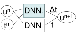
Figure 1. DNN for RK1 (Forward Euler) Scheme

In this and the subsequent figures we have highlighted the ‘important’ or ’essential’ $DNN_{r}$ for $r(u,t)$. The generalization to higher order schemes is given by the family of explicit Runge-Kutta (RK) methods, which may be expressed as:

$$u^{n+1} =u^{n}+{\Delta t}~{}b_{i}~{}r^{i}~{}~{},$$

$$r^{i} =r(t^{n}+c_{i}{\Delta t},~{}u^{n}+{\Delta t}~{}a_{ij}~{}r^{j})~{}~{},~{}~{}i=\overline{1,s},~{}~{}j=\overline{1,s-1}~{}~{}.$$

Any particular RK method is defined by the number of stages $s$ and the coefficients $a_{ij},1\leq j<i\leq s$, $b_{i},i=\overline{1,s}$ and $c_{i},i=\overline{2,s}$. These coefficients are usually arranged in a table known as a Butcher tableau (see Butcher (2003)):

$$\begin{array}[]{c|ccccc}&r^{1}&r^{2}&\dots&r^{s-1}&r^{s}\\ \hline\cr 0&&&&\\ c_{2}&a_{21}&&&&\\ c_{3}&a_{31}&a_{32}&&&\\ \vdots&\vdots&\vdots&\ddots&&\\ c_{s}&a_{s1}&a_{s2}&\dots&a_{s,s-1}&\\ \hline\cr&b_{1}&b_{2}&\dots&b_{s-1}&b_{s}\end{array}$$

The two-step (2nd order) RK scheme is given by:

$$\begin{array}[]{c|cc}&r^{1}&r^{2}\\ \hline\cr 0&&\\ 1/2&1/2&\\ \hline\cr&0&1\end{array}$$

For clarity, let us write the scheme out explicitly:

• Step 1: $u^{n+1/2}=u^{n}+{{\Delta t}\over 2}r(u^{n},t^{n})$

• Step 2: $u^{n+1}=u^{n}+{\Delta t}\,r(u^{n+1/2},t^{n+1/2})$.

The DNN architecture required for this time integration scheme is shown in Figure 2.

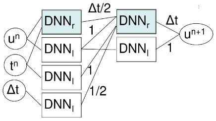
Figure 2. DNN for RK2 Scheme

The classic 4th order RK scheme is given by:

$$\begin{array}[]{c|cccc}&r^{1}&r^{2}&r^{3}&r^{4}\\ \hline\cr 0&&&\\ 1/2&1/2&&&\\ 1/2&0&1/2&&\\ 1&0&0&1&\\ \hline\cr&1/6&1/3&1/3&1/6\end{array}$$

For clarity, let us write the scheme out explicitly:

• Step 1: $u^{n+1/4}=u^{n}+{{\Delta t}\over 2}r(u^{n},t^{n})$

• Step 2: $u^{n+1/3}=u^{n}+{{\Delta t}\over 2}r(u^{n+1/4},t^{n+1/2})$

• Step 3: $u^{n+1/2}=u^{n}+{\Delta t}r(u^{n+1/3},t^{n+1/2})$

• Step 4: $u^{n+1~{}~{}}=u^{n}+$

• ${{\Delta t}\over 6}\left[r(u^{n},t^{n})+2r(u^{n+1/4},t^{n+1/2})+2r(u^{n+1/3},t^{n+1/2})+r(u^{n+1/2},t^{n+1})\right]$.

The DNN architecture required for this time integration scheme is shown in Figure 3.

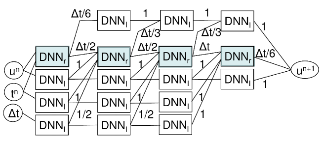
Figure 3. DNN for RK4 Scheme

Observe that schemes of this kind require the storage of several copies of the unknown/right hand side, as the final result requires $r^{i},i=1,s$. Furthermore, as each right-hand side possibly requires the information of all previous right-hand sides of the timestep, the resulting neural net architecture deepens.

5. Example: Mass-Damper-Stiffness System

Consider the simple mass-damper-stiffness system common to structural mechanics, given by the scalar ODE:

$$m\cdot x_{,tt}+d\cdot x_{,t}+c\cdot x=0~{}~{},$$

where $m,d,c,x$ denote the mass, damping, stiffness and displacement respectively. The ODE may be re-written as a first order ODE via:

$$x_{,t}=v~{}~{},~{}~{}v_{,t}=-{d\over m}v-{c\over m}x~{}~{}.$$

The resulting $DNN_{r}$ is shown in Figure 4.

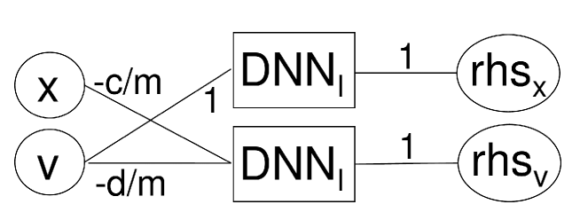
Figure 4. DNN for Mass-Damper-Stiffness System

6. Conclusions and Outlook

Deep neural network (DNN) architectures were constructed that are the exact equivalent of explicit Runge-Kutta schemes for numerical time integration. The network weights and biases are given, i.e., no training is needed. In this way, the only task left for physics-based integrators is the DNN approximation of the right-hand side. This allows to clearly delineate the approximation estimates for right-hand side errors and time integration errors.
As the explicit Runge-Kutta schemes require the information of all previous right-hand sides of the timestep, the resulting neural net architecture depth is proportional to the number of stages - and hence to the integration order of the scheme.
As the DNN for the approximation of the right-hand side may already be ‘deep’, i.e. with several hidden layers, the final DNN for high-order ODE integration many be considerable.

References

- [1] Harbir Antil, Howard C Elman, Akwum Onwunta, and Deepanshu Verma. Novel deep neural networks for solving bayesian statistical inverse problems. arXiv preprint arXiv:2102.03974, 2021.
- [2] Harbir Antil, Ratna Khatri, Rainald Löhner, and Deepanshu Verma. Fractional deep neural network via constrained optimization. Machine Learning: Science and Technology, 2(1):015003, dec 2020.
- [3] Harbir Antil, Rainald Löhner, and Randy Price. NINNs: Nudging Induced Neural Networks. Technical Report arXiv:2203.07947, arXiv, March 2022. arXiv:2203.07947 [cs, math] type: article.
- [4] Sama Bilbao y Leon, Robert Ulfig, and James Blanchard. Neural network theory. Computer Applications in Engineering Education, 4(2):117–125, 1996.
- [5] Ricky TQ Chen, Yulia Rubanova, Jesse Bettencourt, and David K Duvenaud. Neural ordinary differential equations. Advances in neural information processing systems, 31, 2018.
- [6] Ronald DeVore, Boris Hanin, and Guergana Petrova. Neural network approximation. Acta Numerica, 30:327–444, 2021.
- [7] Richard J. Gran. Numerical computing with Simulink. Vol. I. Society for Industrial and Applied Mathematics (SIAM), Philadelphia, PA, 2007. Creating simulations.
- [8] Eldad Haber and Lars Ruthotto. Stable architectures for deep neural networks. Inverse Problems, 34(1):014004, 22, 2018.
- [9] Juncai He, Lin Li, Jinchao Xu, and Chunyue Zheng. Relu deep neural networks and linear finite elements. arXiv preprint arXiv:1807.03973, 2018.
- [10] ST Huseynov. Methodology of laboratory workshops on computer modeling with programming in microsoft excel visual basic for applications. In 2013 7th International Conference on Application of Information and Communication Technologies, pages 1–5. IEEE, 2013.
- [11] Philipp Christian Petersen. Neural network theory. University of Vienna, 2020.
- [12] Maziar Raissi, Paris Perdikaris, and George E Karniadakis. Physics-informed neural networks: A deep learning framework for solving forward and inverse problems involving nonlinear partial differential equations. Journal of Computational Physics, 378:686–707, 2019.
- [13] Lawrence F Shampine, Mark W Reichelt, and Jacek A Kierzenka. Solving index-1 daes in matlab and simulink. SIAM review, 41(3):538–552, 1999.
- [14] Stephen Wolfram. Cellular automata as models of complexity. Nature, 311(5985):419–424, 1984.
- [15] Stephen Wolfram and M Gad-el Hak. A new kind of science. Appl. Mech. Rev., 56(2):B18–B19, 2003.
- [16] Dmitry Yarotsky. Error bounds for approximations with deep relu networks. Neural Networks, 94:103–114, 2017.