Radial velocity confirmation of a hot super-Neptune discovered by TESS with a warm Saturn-mass companion

Abstract

We report the discovery and confirmation of the planetary system TOI-1288. This late G dwarf harbours two planets: TOI-1288 b and TOI-1288 c. We combine TESS space-borne and ground-based transit photometry with HARPS-N and HIRES high-precision Doppler measurements, which we use to constrain the masses of both planets in the system and the radius of planet b. TOI-1288 b has a period of $2.699835^{+0.000004}_{-0.000003}$ d, a radius of $5.24\pm 0.09$ R_⊕, and a mass of $42\pm 3$ M_⊕, making this planet a hot transiting super-Neptune situated right in the Neptunian desert. This desert refers to a paucity of Neptune-sized planets on short period orbits. Our 2.4-year-long Doppler monitoring of TOI-1288 revealed the presence of a Saturn-mass planet on a moderately eccentric orbit ($0.13^{+0.07}_{-0.09}$) with a minimum mass of $84\pm 7$ M_⊕ and a period of $443^{+11}_{-13}$ d. The 5 sectors worth of TESS data do not cover our expected mid-transit time for TOI-1288 c, and we do not detect a transit for this planet in these sectors.

1 Introduction

As the tally of exoplanets has now surpassed 5,000, we can make more informed inferences about planet formation and evolution. A wealth of architectures and different planet types have been discovered, some of which are quite different from the planets found in the Solar System. We first learned about giant planets on short period orbits, the so-called hot Jupiters, which have been found in abundance, owing to their detection bias. The Kepler space mission (Borucki et al., 2010) showed us that, while super-Earths appear to be quite common (Howard et al., 2010a; Mayor et al., 2011), we see a significant dearth of Neptune mass planets on short period orbits, a paucity referred to as the Neptunian “desert” (Mazeh et al., 2016).

In addition to this paucity, studies on the planetary initial mass function (e.g., Mordasini et al., 2009) have found a minimum in the mass range where super-Neptunes reside, namely from around 30 M_⊕ to 70 M_⊕. This valley has been interpreted as the division between planets dominated by solids and gas giants that have undergone runaway gas accretion (Ida & Lin, 2004). Finding and characterising planets in this mass range could therefore help shed light on why some proto-planets undergo runaway accretion while others do not.

Most of the super-Neptunes were detected by Kepler around relatively faint stars, meaning that precise mass determinations only exist for a few of these (e.g., Kepler-101b, Bonomo et al., 2014). The Transiting Exoplanet Survey Satellite (TESS; Ricker et al., 2015) along with ground-based efforts have now detected more of these super-Neptunes in brighter systems for which precise radial velocities (RVs) are more viable, enabling both radius and mass determinations. Therefore, we can also determine the bulk density and make inferences about the composition. A way to gain more insight into the composition and potential migration is through atmospheric studies, which have also been used as a means to rule out certain mechanisms. For instance, as in Vissapragada et al. (2022) in which photoevaporation is ruled out as the mechanism responsible for shaping the upper edge of the Neptunian desert.

Here we report on the discovery and characterisation of the TOI-1288 planetary system. In this system we have discovered a hot super-Neptune, TOI-1288 b, with an outer Saturn mass companion, TOI-1288 c. These planets are hosted by a late G dwarf.

The paper is structured as follows. In Section 2 we describe our observations, which include ground-based photometry as well as that from TESS. We have also acquired speckle and adaptive optics (AO) imaging to search for blended companions. In addition we have carried out extensive spectroscopic follow-up to confirm and characterise this planetary system. In Section 3 we present our analysis of the data in which we model the photometry and spectroscopy jointly. The results are presented in Section 4 and we discuss them in Section 5. Finally, we give our conclusions in Section 6.

Table 1: System parameters. Catalog IDs, coordinates, and magnitudes for the TOI-1288 system.

Parameter	Value	Name
TICa	365733349
Gaia DR3b	2245652826430109184
TYCc	4255-1629-1
$\alpha$ (J2000)b	20:52:40.09	Right ascension (R.A.)
$\delta$ (J2000)b	+65:36:31.59	Declination (Dec.)
$\mu_{\alpha}$ (mas yr-1)b	$43.496\pm 0.017$	Proper motion R.A.
$\mu_{\delta}$ (mas yr-1)b	$-68.775\pm 0.017$	Proper motion Dec.
$\varpi$ (mas)b	$8.720\pm 0.013$	Parallax
RV (km s-1)b	$-68.1\pm 0.6$	Radial velocity
$G$b	$10.4507\pm 0.0018$	Gaia $G$ magnitude
$B_{\mathrm{P}}$b	$10.855\pm 0.006$	Gaia $B_{\mathrm{P}}$ magnitude
$R_{\mathrm{P}}$b	$9.873\pm 0.003$	Gaia $R_{\mathrm{P}}$ magnitude
$V$c	$10.44\pm 0.04$	Tycho $V$ magnitude
$B$c	$11.38\pm 0.07$	Tycho $B$ magnitude
$J$d	$9.19\pm 0.02$	2MASS $J$ magnitude
$H$d	$8.84\pm 0.03$	2MASS $H$ magnitude
$K$d	$8.78\pm 0.02$	2MASS $K$ magnitude

• https://exofop.ipac.caltech.edu/tess/.

• Gaia Collaboration et al. (2022).

• Høg et al. (2000).

• Cutri et al. (2003).

2 Observations

The TOI-1288 system has been observed with different space- and ground-based facilities, including both photometric and spectroscopic observations, as well as high-resolution imaging. System parameters for TOI-1288 are summarised in Table 1.

2.1 Photometry

TESS observed TOI-1288 during Sectors 15, 16, 17, 18, and 24 (August 15 to November 27, 2019, and April 16 to May 13, 2020). This candidate was identified by the Science Processing Operation Center (SPOC; Jenkins et al., 2016) team at the NASA Ames Research Center, who searched the light curves, which are extracted through simple aperture photometry (SAP; Twicken et al., 2010; Morris et al., 2020) and processed using the Presearch Data Conditioning (PDC; Smith et al., 2012; Stumpe et al., 2012; Stumpe et al., 2014) algorithm. The SPOC team searches the PDC-SAP light curves for transit-like signals with an adaptive, noise-compensating matched filter (Jenkins, 2002; Jenkins et al., 2010) using a pipeline that iteratively performs multiple transiting planet searches and stops when it fails to find subsequent transit-like signatures above the detection threshold of a signal-to-noise ratio (SNR) of 7.1. The results were published in the Data Validation Report (DVR; Twicken et al., 2018; Li et al., 2019), and as the light curve shows a $\sim$0.25% dip occurring every 2.7 d with an SNR of around 62, it was identified as a TESS Object of Interest (TOI; Guerrero et al., 2021) and given the ID TOI-1288. The results of the difference image centroiding test were also presented in the DVR, which located the source of the transit signal to within $1.3\pm 2.6^{\prime\prime}$ in the Sector 14-26 multi-sector transit search.

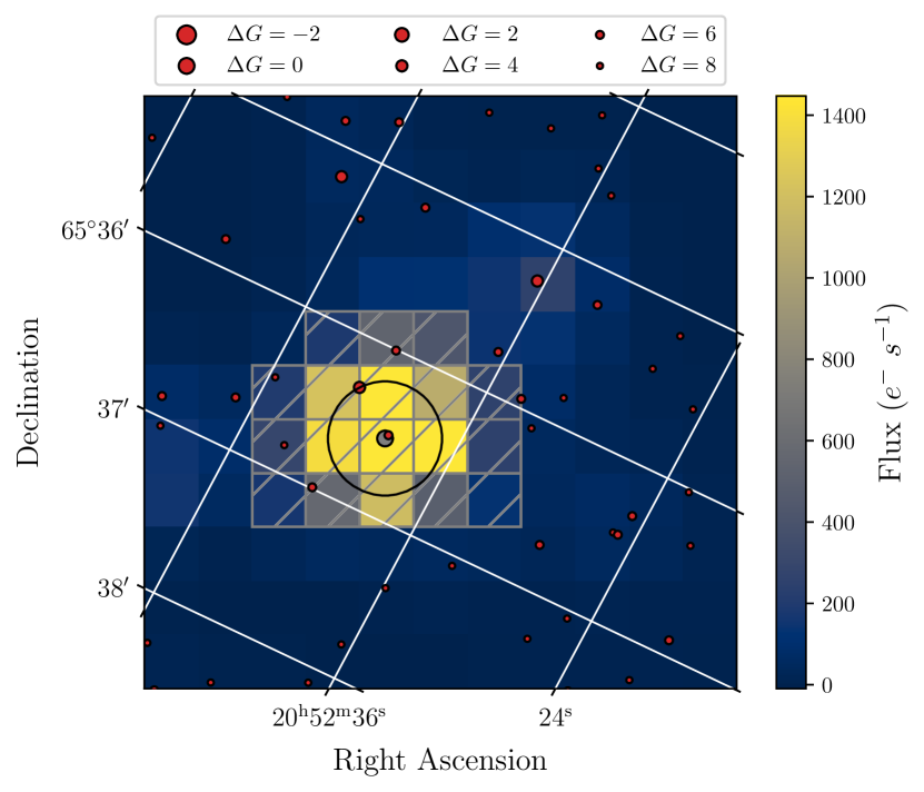
Figure 1: TESS image of TOI-1288. Cutout of a TESS image of TOI-1288 from Sector 15. The red dots denote Gaia sources with their sizes scaled to the difference in $G$ magnitude to TOI-1288. The grey dot denotes the position of TOI-1288. The hatched area shows the aperture mask we used to create the light curves, and the black circle illustrates the separation to the brightest nearby star at $\sim$23 arcsec.

An independent search for transit signals was performed using the Détection Spécialisée de Transits (DST; Cabrera et al., 2012) pipeline on the PDCSAP light curves. A transit signal with orbital period of $2.70\pm 0.02$ days and a transit depth of $\sim$0.25% was detected, consistent with the signal detected by the SPOC pipeline.

Fig. 1 displays the TESS image in the immediate vicinity of TOI-1288 with nearby Gaia DR3 sources (Gaia Collaboration et al., 2022). All the TESS photometry from Sectors 15-18 and Sector 24 is displayed in Fig. 2, where we show the background corrected light curve at the top. This was done using the RegressionCorrector implemented in lightkurve (Lightkurve Collaboration et al., 2018). Overplotted in grey is a model light curve created using batman (Kreidberg, 2015) with transit parameters stemming from an initial fit. We used this to remove the transit signal before removing outliers from the light curve. In the middle light curve the transits are removed, and we have applied a Savitzky-Golay filter (Savitzky & Golay, 1964) to temporarily filter the light curve. We then removed outliers through sigma clipping at 5$\sigma$, these outliers are highlighted in red. Finally, in the bottom light curve we have re-injected the transits to the unfiltered light curve as we want to account for any trend while fitting, as described in Section 3.

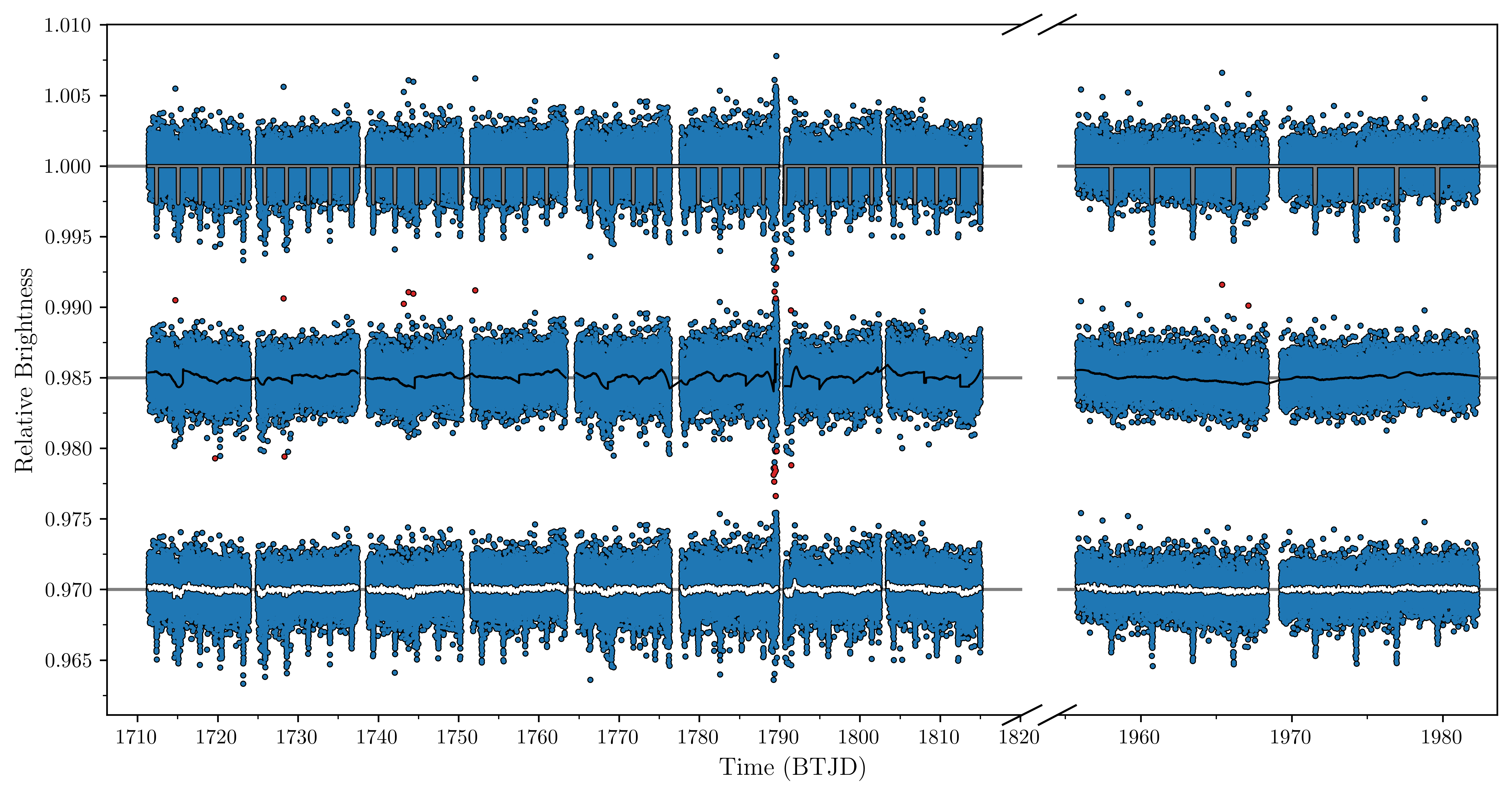
Figure 2: TESS photometry. The light curve at the top shows the background corrected light curve. The grey line is a transit model created from parameters stemming from an initial fit. The transit model has been used to temporarily remove the transit in the light curve shown in the middle. Here the grey line shows a Savitsky-Golay filter (as implemented in Lightkurve Collaboration et al., 2018) used to filter and detrend the data for outlier rejection. The red points are outliers removed through a 5$\sigma$ sigma clipping. The TESS data with outliers removed and the transits re-injected is shown in the light curve at the bottom. The white line is the GP we use to detrend the data (see Section 3).

2.1.1 Light Curve Follow-up

We acquired ground-based time-series follow-up photometry of TOI-1288 as part of the TESS Follow-up Observing Program (TFOP; Collins, 2019) using various facilities as listed in Table 6 from October 2019 to September 2021. This is done in an attempt to (1) rule out or identify nearby eclipsing binaries (NEBs) as potential sources of the detection in the TESS data, (2) detect the transit-like events on target to confirm the depth and thus the TESS photometric deblending factor, (3) refine the TESS ephemeris, and (4) place constraints on transit depth differences across optical filter bands. We used the TESS Transit Finder, which is a customized version of the Tapir software package (Jensen, 2013), to schedule our transit observations. The images were calibrated and the photometric data were extracted using the AstroImageJ (AIJ) software package (Collins et al., 2017), except the Las Cumbres Observatory Global Telescope (LCOGT; Brown et al., 2013) images, which were calibrated by the standard LCOGT BANZAI pipeline (McCully et al., 2018), and the Multicolor Simultaneous Camera for studying Atmospheres of Transiting exoplanets (MuSCAT; Narita et al., 2015) data, which were extracted using the custom pipeline described in (Fukui et al., 2011).

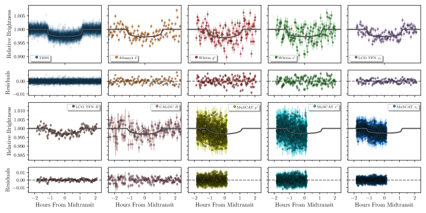
Figure 14: Light curves of TOI-1288 b. The phase folded transits of planet b from all the different photometers. The TESS light curve (top left) is the GP detrended data from Fig. 2. The grey lines are the best-fitting models.

The individual observations are detailed in Table 6 and the light curves are shown in Fig. 14. All photometric apertures exclude flux from all known Gaia DR3 stars near TOI-1288, except the TESS-band 16.4 magnitude neighbor 1.5″southwest, which is nominally too faint to be capable of causing the detection in the TESS photometric aperture (individual follow-up photometric apertures are listed in Table 6). Transit events consistent with the TESS TOI-1288 b transit signal were detected in each light curve and are included in the joint model described in Section 3.

2.2 Speckle/AO imaging

Nearby sources that are blended in the aperture mask used for the photometry can contaminate the light curve and alter the measured radius, it is thus important to vet for close visual companions. Furthermore, a close companion could be the cause of a false positive if the companion is itself an eclipsing binary (Ciardi et al., 2015). We therefore collected both adaptive optics and speckle imaging. The observations are described below and summarised in Table 2.

2.2.1 WIYN/NESSI

On the nights of 2019 November 17 and 2021 October 29, TOI-1288 was observed with the NESSI speckle imager (Scott, 2019), mounted on the 3.5 m WIYN telescope at Kitt Peak, AZ, USA. NESSI simultaneously acquires data in two bands centered at 562 nm and 832 nm using high speed electron-multiplying CCDs (EMCCDs). We collected and reduced the data following the procedures described in Howell et al. (2011). The resulting reconstructed image achieved a contrast of $\Delta\mathrm{mag}\,\approx\,5.75$ at a separation of 1″in the 832 nm band (see Fig. 3).

Figure 3: WIYN/NESSI contrast curves from 2019 (top) and 2021 (bottom). Two filter speckle imaging contrast curves for TOI-1288 from NESSI. The insets show the reconstructed 562 nm and 832 nm images with 1 arcsec scale bars.

On both nights we detected a companion at a separation of $\sim$1.2″, however, only in the 832 nm filter. Additionally, on the night of 2021 October 29 the pipeline detected a companion at a separation of 0.065″(position angle of $313^{\circ}$ and $\Delta\mathrm{mag}=2.57$). However, this companion is close to the detection limit (Scott, 2019), and the fit that produced it relied on image elongation (as opposed to being fully separated from the primary), which is possible to get from a mismatch between the science target and the (single) comparison star. Furthermore, it was not detected in the 2019 November 17 data (despite being of higher quality), nor was it detected in any of the other speckle or AO images (see below). We therefore conclude that the inner companion is a spurious detection most likely caused by a data artifact.

2.2.2 Gemini/’Alopeke

TOI-1288 was observed with the ’Alopeke speckle instrument on the Gemini North telescope, HI, USA, (Scott et al., 2021) on 2020 June 9, 2021 June 24, 2021 October 22, and 2022 May 14 (all dates in UT). Observations were obtained simultaneously in two narrow-band filters centered at 562 nm (width=54 nm) and at 832 nm (width=40 nm). Between 6 and 7 sets of 1000$\times$0.06 s exposures were collected and then reduced with the standard reduction pipeline using Fourier analysis (see, e.g., Howell et al., 2011, for an overview). The reduced data products include reconstructed images and 5$\sigma$ contrast curves. TOI-1288 was very faint in most data sets and even not detected in one of them at 562 nm. At 832 nm, in addition to the primary star, a faint ($\Delta M\sim 5.9$) companion was detected at a projected separation of $\sim$1.2^′′-1.3^′′ in the data from 2020 June 9, 2020 June 24, 2021 October 22, and 2022 May 14. An even fainter ($\Delta M\sim 7$) companion was detected at a separation of $\sim$1.4^′′-1.5^′′ in the data from 2020 June 24, 2021 October 22, and 2022 May 14.

2.2.3 Gemini/NIRI

We collected adaptive optics images of TOI-1288 with the Gemini Near-Infrared Imager (NIRI; Hodapp et al., 2003) on 2019 November 8. We collected 9 science frames, each with an exposure time of 6.8 s, and dithered the telescope by $\sim$2″ between each frame, thereby allowing for the science frames themselves to serve as sky background frames. The target was observed in the Br-$\gamma$ filter centered at 2.166 $\mu$m. Data processing consisted of bad pixel removal, flat fielding, and subtraction of the sky background. We then aligned the frames based on the position of the primary star, and coadded the images.

The total field of view is around 26^′′ square, with optimum sensitivity in the central $\sim$22^′′ square. We again identified two visual candidates in the field of view. The brighter companion is at a separation of 1.152^′′, a position angle of 289.3 degrees counter-clockwise of north, and is 4.77$\pm$0.03 mag fainter than the host in the Br-$\gamma$ band; the fainter companion is at a separation of 1.579^′′, a position angle of 207.7 degrees counter-clockwise of north and is 5.88$\pm$0.04 mag fainter than the host.

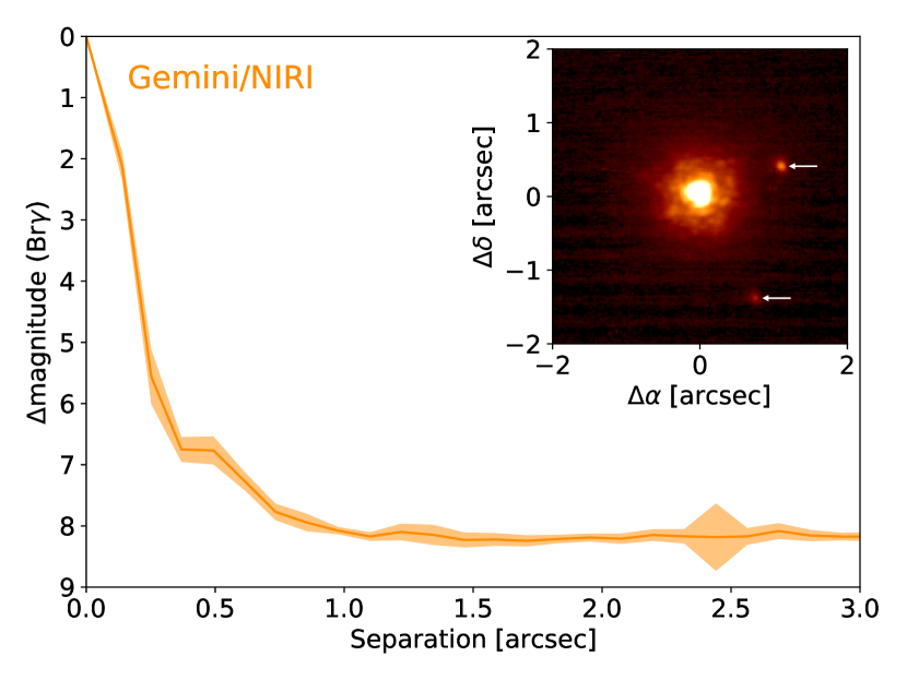
Figure 4: Gemini/NIRI contrast curve. AO imaging contrast curve for TOI-1288. The inset shows the reconstructed Br-$\gamma$ image with the two detected companions highlighted.

We measured the sensitivity of our observations as a function of radius by injecting fake companions and scaling their brightness such that they could be detected at 5$\sigma$. The contrast sensitivity is 5.56 mag fainter than the host at a separation of 250 mas, and 8.1 mag fainter than the host in the background limited regime, beyond $\sim$1^′′ from the target. The contrast sensitivity as a function of radius and a high resolution image of the star are shown in Fig. 4; we show the curve for the inner 3^′′ only, but note that the data are sensitive to candidates within 13^′′ in all directions. From our speckle and AO imaging we have thus identified two nearby companions.

Table 2: Companions detected in Speckle, AO, and Gaia. $\rho$ and $\Delta$ are the separation and the difference in magnitude from the central target (host), respectively. $\theta$ is the position angle from the brighter of the targets to the fainter component, measured from North through East. Star 1 is the brighter companion and star 2 the fainter one. The uncertainties for $\rho$ and $\theta$ for the ’Alopeke data are estimated to be around 5 mas and 1 deg, respectively, while the uncertainties for $\Delta$mag come out to around 0.5 mag for the closer companion and 1 mag for the fainter one.

Date	Star	$\rho$	$\Delta$	$\theta$	Type	Filter	Instrument	Telescope
(UT)		(arcsec)	(mag)	(deg)
2019-11-08	1	1.152	$4.77\pm 0.03$	289.3	AO	Br-$\gamma$	NIRI	Gemini
2019-11-08	2	1.579	$5.88\pm 0.04$	207.7	AO	Br-$\gamma$	NIRI	Gemini
2019-11-17a	1	1.123	5.90	289.5	Speckle	832 nm	NESSI	WIYN
2020-06-09a	1	1.172	5.94	289.5	Speckle	832 nm	’Alopeke	Gemini
2021-06-24a	1	1.256	6.4	292.0	Speckle	832 nm	’Alopeke	Gemini
2021-06-24a	2	1.516	6.8	211.7	Speckle	832 nm	’Alopeke	Gemini
2021-10-22a	1	1.233	5.92	293.4	Speckle	832 nm	’Alopeke	Gemini
2021-10-22a	2	1.468	7.34	212.3	Speckle	832 nm	’Alopeke	Gemini
2021-10-29a	1	1.282	5.48	293.6	Speckle	832 nm	NESSI	WIYN
2022-05-14a	1	1.306	5.83	293.5	Speckle	832 nm	’Alopeke	Gemini
2022-05-14a	2	1.443	7.90	214.3	Speckle	832 nm	’Alopeke	Gemini
Epoch=2016.0	2	1.74	6.41	198	Photometry	$G$	-	Gaia

• Observations were also carried out in the 562 nm filter, but the companions were not detected in this filter.

2.2.4 Gaia

As is also apparent from Fig. 1, one of the two aforementioned companions is also detected by Gaia DR3. The position of this Gaia companion is in good agreement with it being the fainter of the two companions seen in the Gemini ’Alopeke and AO observations. This is most likely also the companion seen in the light curve follow-up in Section 2.1.1. The Gaia detection is summarised in Table 2 along with the speckle and AO observations.

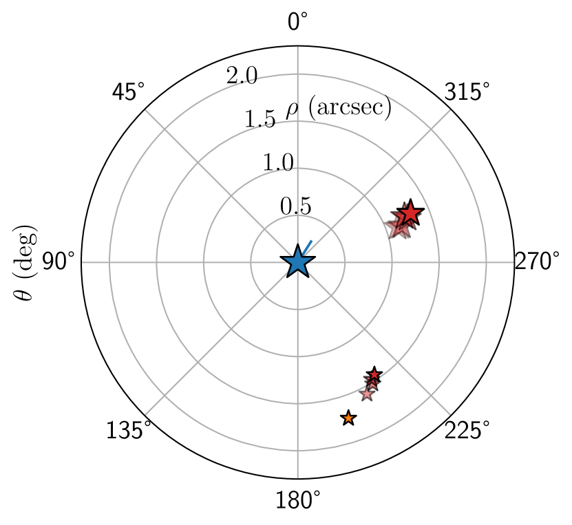
Figure 5: Sky positions of blended companions. The blue star denotes TOI-1288, while red stars are the relative positions for the companions detected in the Spekle/AO images. Their sizes are scaled according to their relative brightness with the larger stars corresponding to $\Delta$Br-$\gamma=4.77$ and the smaller one corresponding to $\Delta$Br-$\gamma=5.88$. The transparent trails show how the companions move relative to TOI-1288 as a function of time with the opaque being the most recent position. The orange star is the relative position of the companion detected by Gaia, which is most likely the fainter companion. The blue line shows the proper motion of TOI-1288 over the course of 3.5 years.

2.2.5 Are the companions bound?

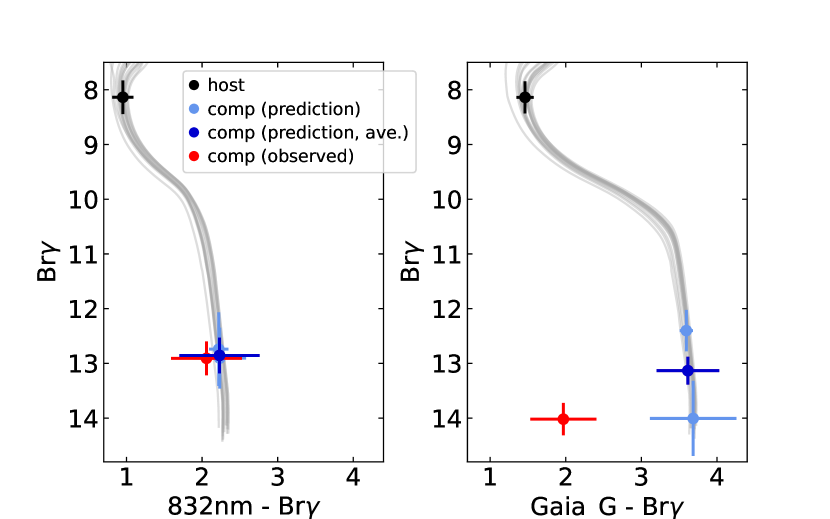
Figure 15: Colour-magnitude diagrams for TOI-1288. Comparison of observed photometry with predicted photometry for both candidate companions. In each case, we show the CMD position of the host (black), the predicted position of a bound companion based on each measured $\Delta$mag (light blue) and the weighted average of these predictions (dark blue), and finally the observed CMD position of the companion (red). The clear disagreement for star 2 (right) indicates that this is a background object, while the relative agreement between the red and dark blue points for star 1 (left) could indicate a bound companion. As discussed in Section 2.2.5 this is not the case.

In the following we will be referring to the brighter companion as star 1, and the fainter companion as star 2. To test whether these companions are bound, we study the positions of the host and the candidate companion in colour-magnitude diagrams (CMDs), loosely following the method outlined in Hirsch et al. (2017). We used the measured photometry in the 832 nm and Br-$\gamma$ filters for star 1, and the Gaia $G$ and Br-$\gamma$ filters for star 2. In each case, we used the stellar parameters and uncertainties of the host ($\tau_{\star}$, [Fe/H], $\log g$, and $d$ from the SED fit in Table 3) to generate a set of 1000 randomly sampled isochrones. For each filter pair, we determined a companion CMD position from the set of isochrones based on the $\Delta$-magnitude of the companion in each filter, and then calculated a weighted average of these measurements. This can then be compared to the observed CMD position of the companion as seen in Fig. 15. For star 1, the observed and predicted positions agree to within 0.3$\sigma$, which could indicate that these objects are bound. This is further supported by their relative proximity on the sky. However, this could also be chance alignment for a background star with the right colour profile (Hirsch et al., 2017). For star 2, the observed and predicted CMD positions do not match, with a disagreement of 3.5$\sigma$. This strongly suggests that star 2 is a background star, and is not physically bound to the TOI-1288 system.

In Fig. 5 we show the relative positions of the companions detected in Speckle/AO and the one detected in Gaia. Evidently, the detected companions seem to be moving over the time span covered by the different observations in a similar direction, which is more or less opposite to the proper motion of TOI-1288. This clearly suggests that neither of the two companions are bound and are likely background stars. Finally, we note that the Gaia position is an average of different scans taken from July 2014 to May 2017 (for DR3) and might be less reliable. Furthermore, the reason that only the fainter companion was detected in the Gaia data could be that at an earlier epoch TOI-1288 and the brighter companion star were likely closer on the sky, and it would thus have been more difficult for Gaia to detect this companion. However, as seen in the speckle/AO observations, due to the proper motion of TOI-1288, the separation between TOI-1288 and this background star is increasing, meaning that it might be possible to detect it in future data releases.

2.3 High-resolution spectroscopy

2.3.1 FIES

We performed high-resolution (R = $67\,000$) reconnaissance spectroscopy of TOI-1288 using the FIber-fed Echelle Spectrograph (FIES; Frandsen & Lindberg, 1999; Telting et al., 2014) mounted at the Nordic Optical Telescope (NOT; Djupvik & Andersen, 2010) at Roque de los Muchachos Observatory, La Palma, Spain. The FIES spectra were extracted following Buchhave et al. (2010), and stellar parameters were derived using the stellar parameter classification (SPC; Buchhave et al., 2012, 2014) tool. The resulting parameters are tabulated in Table 3.

2.3.2 HARPS-N

We acquired 57 high-resolution (R = 115 000) spectra of TOI-1288 utilizing the High Accuracy Radial velocity Planetary Searcher for the Northern hemisphere (HARPS-N; Cosentino et al., 2012) attached at the 3.58 m Telescopio Nazionale Galileo (TNG), also located at Roque de los Muchachos observatory. The spectra were collected between 19 November 2019 and 23 May 2022. We set the exposure time to 1200-2700 s based on the sky conditions and scheduling constraints, which led to a median SNR of $\sim$60 per pixel at 550 nm. We used the second fibre of the instrument to monitor the sky background.

The HARPS-N spectra were reduced and extracted using the dedicated Data Reduction Software (DRS; Lovis & Pepe, 2007) available at the telescope. The DRS also provides the full width at half maximum (FWHM) and the bisector inverse slope (BIS) of the cross-correlation function (CCF), which was obtained by cross-correlating the observed échelle spectra against a G2 numerical mask. In this work, we used the Template-Enhanced Radial velocity Re-analysis Application (TERRA; Anglada-Escudé & Butler, 2012) to extract precise RV measurements, along with additional activity indicators (namely, the H$\alpha$, S-index, and Na D indexes).

2.3.3 HIRES

We also gathered 28 spectra the High Resolution Echelle Spectrometer (HIRES; Vogt et al., 1994) mounted on the 10 m Keck-1 at the Keck Observatory, Hawai’i, USA. Observations were carried out between 10 December 2019 and 11 October 2021 with exposure times varying from 280-1000 s depending on sky conditions, resulting in a median SNR of $\sim$72 near the spectral center of the image. The spectra were obtained with the iodine cell in the light path, and the RV extraction followed the standard HIRES forward-modelling pipeline (Howard et al., 2010b).

2.3.4 Periodogram Analysis

All the RVs are shown in Fig. 6 and tabulated in Table 7. In Fig. 7 we have calculated the generalised Lomb-Scargle (GLS; Lomb, 1976; Scargle, 1982) periodogram. Evidently, the $\sim$2.7 d transiting signal is also detected in the RVs, where a peak at this frequency clearly exceeds the false-alarm probabilities (FAPs; at 0.1%, 1%, and 10%). We also see a significant peak at much lower frequencies with a period of around $443$ d, which we ascribe to the presence of a further out companion. Seeing the $443$ d-signal we searched the TESS light curve for additional transits using the box least squares (BLS; Kovács et al., 2002) algorithm after removing the transits from planet b ($\sim$2.7 d), but found no evidence for additional transiting signals.

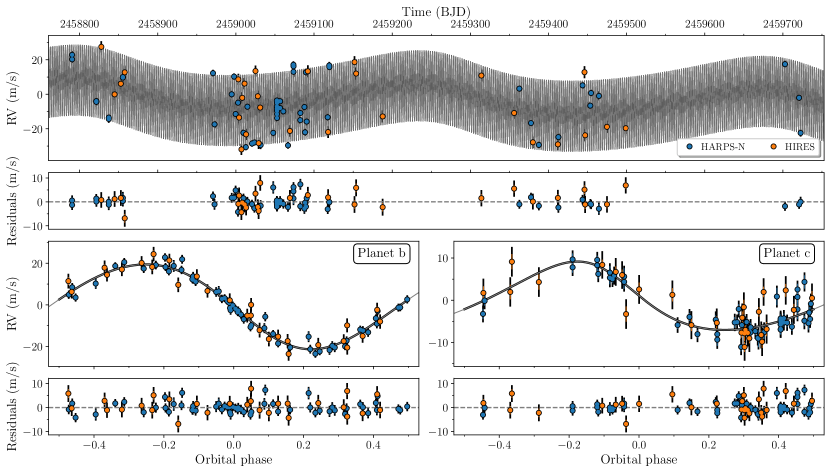
Figure 6: Radial velocities of TOI-1288. Top: The HARPS-N (blue) and HIRES (orange) radial velocities as a function time. The grey model shows the combined signal for planet b and c. Bottom left: The radial velocities phased to the period planet b with the signal from planet c and the long-term trend subtracted with the best-fitting model overplotted. Bottom right: The radial velocities phased to the period of planet c with the signal from planet b and the long-term trend subtracted with the best-fitting model overplotted.

We also detected another low frequency/long period peak in the GLS which seems to be a long-term trend in the RVs. We have furthermore created GLS periodograms for the activity indicators from the HARPS-N spectra shown in Fig. 8. Evidently, the star is inactive and the 2.7 d and $443$ d do not coincide with any appreciable peak in these metrics, meaning that they are unlikely to come from stellar activity.

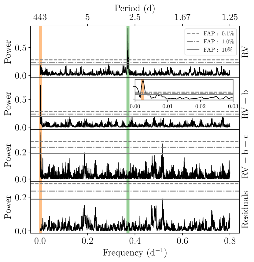
Figure 7: Generalised Lomb-Scargle diagram. The GLS created from the RVs in Table 7. Top: The GLS after subtracting the systemic velocities for HARPS-N and HIRES. The periods from Table 4 for planet b (green) and planet c (orange) are shown as the vertical lines. The dashed, dashed-dotted, and solid horizontal lines are the 0.1%, 1%, and 10% FAPs, respectively. Upper middle: The GLS after subtracting the signal from planet b. The inset shows a close-up around the period of planet c. Lower middle: The GLS after subtracting both the signal from planet b and c. Lower: The GLS after subtracting both the signal from planet b, c, and the long-term trend.

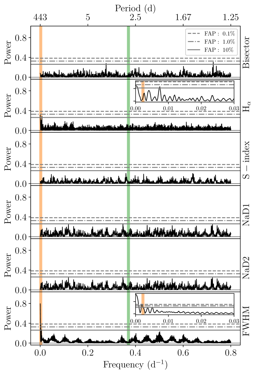
Figure 8: Generalised Lomb-Scargle diagram for activity indicators. The GLS created from the activity indicators from the HARPS-N spectra. From top to bottom we show the GLS for the Bisector, H_α, S-index, NaD1, NaD2, and full width half maximum (FWHM). Symbols have the same meaning as in Fig. 7.

2.3.5 Stellar modelling using SME and SED

In addition to the FIES reconnaissance spectroscopy we also made use of our HARPS-N observations to derive stellar properties. We used co-added HARPS-N spectra with the software SME (Spectroscopy Made Easy; Valenti & Piskunov, 1996; Piskunov & Valenti, 2017), a tool for fitting observations to synthetic spectra. A detailed description of the modelling can be found in Fridlund et al. (2017) and Persson et al. (2018). For this star, we held the micro- and macro-turbulent velocities, $v_{\rm mic}$ and $v_{\rm mac}$, fixed in the modelling to 0.83 km s^-1 (Bruntt et al., 2010), and 3.0 km s^-1 (Doyle et al., 2014), respectively. The synthetic spectra were computed with the stellar atmosphere grid Atlas12 (Kurucz, 2013), and the atomic and molecular line data were taken from VALD (Ryabchikova et al., 2015). Our best model found an effective temperature of $T_{\rm eff}=5123\pm 62$ K, an iron abundance of [Fe/H]$=+0.10\pm 0.11$, a surface gravity of $\log g_{\star}=4.23\pm 0.09$, and a projected rotational velocity of $v\sin i_{\star}=1.3\pm 1.2$ km s^-1. These results were checked with the empirical code SpecMatch-Emp (Yee et al., 2017) and were found to agree within $1~{}\sigma$.

Using the SME results as priors, we modelled the stellar radius with ARIADNE (Vines & Jenkins, 2022) fitting broadband photometry to the spectral energy distribution (SED). The fitted bandpasses were the Johnson $B$ and $V$ magnitudes (APASS), $GG_{\rm BP}G_{\rm RP}$ (eDR3), $JHK_{S}$ magnitudes (2MASS), WISE W1-W2, and the Gaia eDR3 parallax. The final radius was computed with Bayesian Model Averaging from the four fitted atmospheric models grids Phoenix v2 (Husser et al., 2013), BtSettl (Allard et al., 2012), Castelli & Kurucz (2004), and Kurucz (1993) atmospheric model grids. The final stellar radius was found to be $1.010\pm 0.015$ $R_{\odot}$, and the stellar mass $0.895^{+0.042}_{-0.023}$ $M_{\odot}$ interpolated from the MIST (Choi et al., 2016) isochrones. The stellar parameters are summarised in Table 3.

2.3.6 Stellar modelling using BASTA

As an independent measure for the stellar parameters we also modelled the star using the BAyesian STellar Algorithm (BASTA; Silva Aguirre et al., 2015; Aguirre Børsen-Koch et al., 2022). We ran BASTA using the spectroscopic parameters from the SPC analysis ($T_{\rm eff}$, [Fe/H], $\log g$) as input along with the Gaia magnitudes ($G$, $B_{\rm P}$, $R_{\rm P}$) and parallax. BASTA’s approach to fitting the magnitudes and parallax is described in Section 4.2.2 in Aguirre Børsen-Koch et al. (2022), where bolometric corrections are applied using the tables by Hidalgo et al. (2018), and the reddening is calculated through the dust map by Green et al. (2019). BASTA uses these values as constraints when fitting to a grid of BaSTI (a Bag of Stellar Tracks and Isochrones; Hidalgo et al., 2018) isochrones, where we opted for a science case that included both diffusion, convective core overshooting, and mass loss (see Section 3.1 in Aguirre Børsen-Koch et al., 2022). The resulting values are tabulated in Table 3 and are generally consistent with the other parameters, although BASTA found a slightly smaller stellar radius as the fit seemed to prefer a slightly larger value for $\log g$ compared to the SME and SED fits.

In the following we will be using stellar parameters coming from the SED. Therefore, derived quantities such as the planetary radius and masses will be calculated from the SED parameters.

Table 3: Stellar parameters for TOI-1288. The stellar parameters from our spectral analyses and stellar modelling in Section 2.3, Section 2.3.5, and Section 2.3.6. We also list the Gaia measurements.

Parameter	Name	SME	SED	Spec-Match	SPC+BASTAe	Gaia DR3
$T_{\mathrm{eff}}$	Effective temperature (K)	$5123\pm 62$	5225${}^{+23}_{-27}$	$5220\pm 110$	5367$\pm$ 50	$5300^{+20}_{-22}$
$\log g$	Surface gravity	$4.23\pm 0.09$	$4.24\pm 0.09$	$4.36\pm 0.12$	$4.36\pm 0.10$	$4.447^{+0.010}_{-0.006}$
$\rm[Fe/H]$	Iron abundance	$0.10\pm 0.11$	$0.07\pm 0.09$	$0.30\pm 0.09$	$0.18\pm 0.08$	$0.15^{+0.02}_{-0.03}$
$\rm[Ca/H]$	Calcium abundance	$0.15\pm 0.09$	-	-	-	-
$\rm[Na/H]$	Sodium abundance	$0.25\pm 0.12$	-	-	-	-
$v\sin i_{\star}$	Projected rotation velocity (km s-1)	$1.3\pm 1.2$	-	-	<2	-
$\zeta$	Macro-turbulence (km s-1)	3.0a	-	-	-	-
$\xi$	Micro-turbulence (km s-1)	0.83b	-	-	-	-
$d$	Distance (pc)	-	114.7 $\pm$ 0.7	-	$112.8^{+1.6}_{-1.4}$	$114.677\pm 0.013$
$R_{\star}$	Stellar radius (R⊙)	-	1.010${}^{+0.015}_{-0.014}$	$1.09\pm 0.18$	$0.95_{-0.02}^{+0.03}$	-
$M_{\star}$c	Stellar mass (M⊙)	-	0.89${}^{+0.04}_{-0.02}$	0.90 $\pm$ 0.08	$0.91^{+0.04}_{-0.05}$	-
$M_{\star}$d	Stellar mass (M⊙)	-	0.65${}^{+0.14}_{-0.13}$	-	-	-
$L_{\star}$	Luminosity (L⊙)	-	$0.68\pm 0.02$	-	$0.65\pm 0.03$	-
$A_{V}$	$V$ band extinction	-	0.014${}^{+0.015}_{-0.009}$	-	-	-
$\tau_{\star}$	Age (Gyr)	-	12.1${}^{+1.4}_{-3.1}$	$10.05\pm 0.17$	$9.8^{+4.7}_{-3.8}$	-

• Relation from Doyle et al. (2014).

• Relation from Bruntt et al. (2010).

• SED estimate is from MIST isochrones.

• SED estimate is from $\log g$ and $R_{\star}$.

• $T_{\rm eff}$, $\log g$, [Fe/H], and $v\sin i_{\star}$ are from SPC. The rest have been derived using BASTA.

3 Analysis

In our modelling we included both planets, where only parameters for planet b are constrained by the photometry given we have not detected any transits of planet c. We modelled the transits using batman, where we accounted for the correlated noise in the light curve using Gaussian Process (GP) regression as implemented in celerite (Foreman-Mackey et al., 2017). We made use of the Matèrn-3/2 kernel, which is characterised by two hyper parameters: the amplitude, $A$, and the time scale, $\tau$. This model is shown at the bottom of Fig. 2.

In addition to the RV signals from planet b and c, we included a first-order acceleration parameter, $\dot{\gamma}$, to account for the long-term trend. Instead of stepping in $e$ and $\omega$, our Markov Chain Monte Carlo (MCMC) sampling was stepping in $\sqrt{e}\cos\omega$ and $\sqrt{e}\sin\omega$ for both planets. Furthermore, we were stepping in the sum of the limb-darkening coefficients, $q_{1}+q_{2}$, while keeping the difference fixed. All stepping parameters and their priors are listed in Table 4.

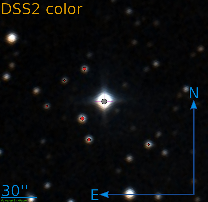
Figure 16: DSS2 image of TOI-1288. The field around TOI-1288 as seen by the Digitized Sky Survey (DSS2). TOI-1288 is marked with the grey dot, and the red dots are the stars within the aperture in Fig. 1 using the same (relative) scaling for the marker sizes.

As seen in Fig. 1 (see also Fig. 16 for a DSS2 image of the field) there are multiple companions in the TESS aperture mask. Therefore we added a dilution term in the MCMC, where we only included the contribution from all sources brighter than $\Delta G=5$, meaning that only the contribution from the south-eastern companion at a separation of $\sim$23 arcsec (Fig. 1) was included. We thus did not consider the contribution from the (much closer) companions. The brightest of the two is found at $\Delta$Br-$\gamma=4.77\pm 0.03$ and from our measurements in Table 2 it is clear that both companions seem to be redder than TOI-1288, meaning that the differences in magnitude are even larger in the TESS passband.

The total flux as a function of time is thus $F(t)=(F_{1}(t)+F_{2})/(F_{1}+F_{2})$, where $F_{1}(t)$ is the in-transit flux and $F_{1}$ is the out-of-transit flux for TOI-1288, and $F_{2}$ is the flux from the contaminating source at $\sim$23 arcsec. The flux from the contaminating source is then included as a fraction of TOI-1288, $F_{1}/F_{2}$, which in magnitude translates to $\Delta\mathrm{mag}=-2.5\log(F_{2}/F_{1})$. As the TESS passband is very close to the Gaia $R_{\mathrm{P}}$ passband, we used the difference in this passband as a proxy for the difference between TOI-1288 and the 23 arcsec neighbour in the TESS passband. Thus we sampled the dilution as a Gaussian prior with $\Delta R_{\mathrm{P}}=\Delta\mathrm{TESS}=4.41\pm 0.02$. The photometric apertures from the ground-based facilities are small enough (Table 6) so that this source does not contaminate those light curves. As such no dilution factors were included for these.

We sampled the posteriors for the transit and orbital parameters using MCMC sampling utilising the emcee package (Foreman-Mackey et al., 2013). Our likelihood function is defined as

$$\log\mathcal{L}=-0.5\sum_{i=1}^{N}\left[\frac{(O_{i}-C_{i})^{2}}{\sigma_{i}^{2}}+\log 2\pi\sigma_{i}^{2}\right]\,,$$ (1)

where $N$ indicates the total number of data points from photometry and RVs. $C_{i}$ represents the model corresponding to the observed data point $O_{i}$. $\sigma_{i}$ represents the uncertainty for the $i$th datum, where we add a jitter term in quadrature and a penalty in the likelihood for the RVs. To our likelihood in Eq. (1) we add our priors $\sum_{j=1}^{M}\log\mathcal{P}_{j}$, $\mathcal{P}_{j}$ being the prior on the $j$th parameter, and this sum constitutes the total probability.

Table 4: MCMC results. The median and high posterior density at a confidence level of 0.68. Subscripts b and c denote parameters for planet b and c, respectively. $\mathcal{U}$ denotes that a uniform prior was applied during the run.

Parameter	Name	Prior	Value
Stepping parameters
$P_{\mathrm{b}}$	Period (days)	$\mathcal{U}$	$2.699835^{+0.000004}_{-0.000003}$
$T_{\mathrm{0,b}}$	Mid-transit time (BTJD)	$\mathcal{U}$	$1712.3587\pm 0.0002$
$(R_{\mathrm{p}}/R_{\star})_{\mathrm{b}}$	Planet-to-star radius ratio	$\mathcal{U}$	$0.0476\pm 0.0005$
$(a/R_{\star})_{\mathrm{b}}$	Semi-major axis to star radius ratio	$\mathcal{U}$	$8.5\pm 0.4$
$K_{\mathrm{b}}$	Velocity semi-amplitude (m s-1)	$\mathcal{U}$	$20.7^{+0.4}_{-0.5}$
$\cos i_{\mathrm{b}}$	Cosine of inclination	$\mathcal{U}$	$0.030^{+0.012}_{-0.030}$
$(\sqrt{e}\cos\omega)_{\mathrm{b}}$		$\mathcal{U}$	$-0.19^{+0.03}_{-0.04}$
$(\sqrt{e}\sin\omega)_{\mathrm{b}}$		$\mathcal{U}$	$0.16^{+0.07}_{-0.06}$
$P_{\mathrm{c}}$	Period (days)	$\mathcal{U}$	$443^{+11}_{-13}$
$T_{\mathrm{0,c}}$	Mid-transit time (BTJD)	$\mathcal{U}$	$1883^{+12}_{-14}$
$K_{\mathrm{c}}$	Velocity semi-amplitude (m s-1)	$\mathcal{U}$	$7.6^{+0.5}_{-0.6}$
$(\sqrt{e}\cos\omega)_{\mathrm{c}}$		$\mathcal{U}$	$0.15^{+0.19}_{-0.15}$
$(\sqrt{e}\sin\omega)_{\mathrm{c}}$		$\mathcal{U}$	$0.28^{+0.14}_{-0.13}$
$\gamma_{\mathrm{HARPS-N}}$	Systemic velocity HARPS-N (m s-1)	$\mathcal{U}$	$7.7^{+0.8}_{-0.7}$
$\sigma_{\mathrm{HARPS-N}}$	Jitter HARPS-N (m s-1)	$\mathcal{U}$	$1.9\pm 0.3$
$\gamma_{\mathrm{HIRES}}$	Systemic velocity HIRES (m s-1)	$\mathcal{U}$	$6.2^{+0.9}_{-1.0}$
$\sigma_{\mathrm{HIRES}}$	Jitter HIRES (m s-1)	$\mathcal{U}$	$3.4\pm 0.6$
$\dot{\gamma}$	Linear trend (m s-1 d-1)	$\mathcal{U}$	$-0.0088\pm 0.0017$
Derived parameters
$e_{\mathrm{b}}$	Eccentricity	-	$0.064^{+0.014}_{-0.015}$
$\omega_{\mathrm{b}}$	Argument of periastron (∘)	-	$139^{+13}_{-17}$
$i_{\mathrm{b}}$	Inclination (∘)	-	$88.3^{+1.7}_{-0.7}$
$b_{\mathrm{b}}$	Impact parameter	-	$0.26^{+0.10}_{-0.24}$
$e_{\mathrm{c}}$	Eccentricity	-	$0.13^{+0.07}_{-0.09}$
$\omega_{\mathrm{c}}$	Argument of periastron (∘)	-	$63^{+30}_{-33}$
$T_{\mathrm{14,b}}$	Transit duration (hours)	-	$2.37_{-0.03}^{+0.05}$
Physical parameters †
$T_{\mathrm{eq,b}}$$\chi$	Equilibrium temperature (K)	-	$1266\pm 27$
$R_{\mathrm{p,b}}$	Planet radius (R⊕)	-	$5.24\pm 0.09$
$M_{\mathrm{p,b}}$	Planet mass (M⊕)	-	$42\pm 3$
$\rho_{\mathrm{p,b}}$	Planet density (g cm-3)	-	$1.3\pm 0.5$
$(M_{\mathrm{p}}\sin i)_{\mathrm{c}}$	Lower value for planet mass (M⊕)	-	$84\pm 7$

• Barycentric TESS Julian Date (BTJD) is defined as BJD-2457000.0, BJD being the Barycentric Julian Date

• From the SED stellar parameters in Table 3.

• Following Kempton et al. (2018).

4 Results

In Fig. 9 we show the TESS light curve phase-folded on the transits of planet b along with the best-fitting model. Light curves from all photometric observations can be found in Fig. 14. We find a planet-to-star radius ratio of $0.0476\pm 0.0005$, which given the stellar radius from the SED analysis in Table 3 yields a radius of $5.24\pm 0.09$ R_⊕. With a period of just $2.699835^{+0.000004}_{-0.000003}$ d, TOI-1288 b is thus a hot super-Neptune.

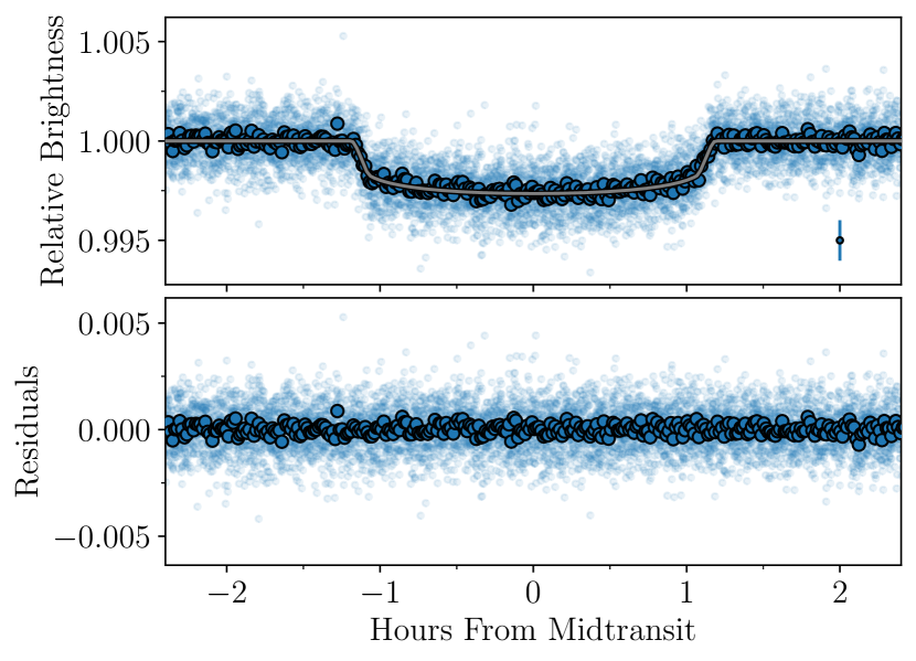
Figure 9: TESS light curve of TOI-1288 b. The GP detrended TESS data from Fig. 2 showing the phase folded transits of planet b. We show the data binned in larger, solid points, while the unbinned data are shown smaller, more transparent points. The datum with errorbar is not an actual measurement, but illustrates the median of the uncertainties of all data. The grey line is the best-fitting model.

Shown in Fig. 6 are the best-fitting models for the radial velocities for both planet b and c. This 2-planet model is heavily favoured over a 1-planet model according to the Bayesian information criterion (BIC, $\Delta$BIC$=104$). To get a measure of the mass for both planets we use the relation

$$M_{\rm p}\sin i=\frac{K\sqrt{1-e^{2}}}{28.4~{}\mathrm{m}~{}\mathrm{s}^{-1}}\left(\frac{P}{1~{}\mathrm{yr}}\right)^{1/3}\left(\frac{M_{\star}}{\mathrm{M}_{\odot}}\right)^{2/3}\,,$$ (2)

where we can only get a lower limit for the mass of planet c as we do not know the inclination. For planet b we find a mass of $42\pm 3$ M_⊕, which combined with the radius yields a bulk density of $1.3\pm 0.5$ g cm^-3. For planet c we find a lower limit for the mass of $84\pm 7$ M_⊕.

For the long-term trend we have found a value for $\dot{\gamma}=-0.0086\pm 0.0019$ m s^-1 d^-1. This first-order acceleration parameter constitutes a lower limit for the semi-amplitude through $(t_{\rm f}-t_{\rm i})\times\dot{\gamma}/2$ with $t_{\rm f}$ and $t_{\rm i}$ being the final and first timestamps. Following the Monte Carlo approach in Kane et al. (2019) (see also Pepper et al., 2020), we used our measured value for $\dot{\gamma}$ to calculate the lower limit for the companion inducing this long-term trend as a function of orbital separation. Namely, we solved

$$K\leq\sqrt{\frac{G}{a_{\rm B}(1-e_{\rm B}^{2})}}\frac{M_{\rm B}\sin i_{\rm B}}{\sqrt{M_{\rm B}+M_{\star}}}$$ (3)

for M_B at each $a_{\rm B}$ with $e_{\rm B}$ being drawn from a $\beta$-distribution and $\cos i_{\rm B}$ from a uniform distribution.

In Fig. 10 we show the resulting distributions for each orbital separation, here converted to a sky-projected separation. We furthermore show the observed position of the brightest of the two companions, star 1, detected in speckle and AO, if it were bound to TOI-1288. From our analysis in Section 2.2.5 and its position in the CMD in Fig. 15 this companion would most likely have been an M-dwarf with a mass of around $0.2$ M_⊙. While this is a lower limit for the mass and could be consistent with the mass we have estimated for star 1, the median is around two orders of magnitude lower at the position for star 1. We should thus in most cases have detected a much more significant drift, if it were due to star 1. Therefore, it seems more likely that the drift we are seeing is coming from another planetary companion.

Finally, we note that the Gaia Renormalised Unit Weight Error (RUWE) statistic for TOI-1288 is 1.17. For a good single-star fit one would expect it to be around 1, whereas a value of $\gtrapprox 1.4$ could suggest that the source is non-single or otherwise problematic for the astrometric solution. The slight departure could be because the Gaia astrometry is seeing the orbital motion induced by this long-term RV companion.

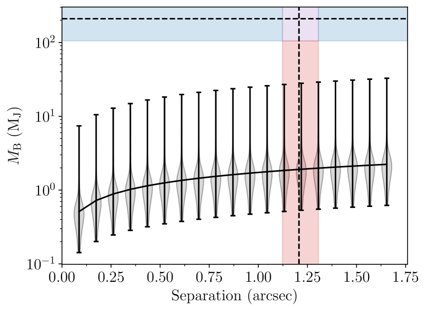
Figure 10: Lower mass limit for an additional bound companion. The violinplot shows the resulting distribution for for the mass of the companion for a given separation (here converted to sky-projected separation using the distance from Table 1). The solid black curve is the median mass for each separation. The vertical red band spans the range of the speckle and AO measurements for the separation of star 1 (Table 2), while the dashed vertical line is the median of these. The horizontal blue band spans the range from 0.1 M_⊙ to 0.3 M_⊙ with 0.2 M_⊙ shown with the dashed line.

5 Discussion

5.1 Location in the Neptunian desert

We have found TOI-1288 b to be a hot super-Neptune with an equilibrium temperature of $1266\pm 27$ K (estimated from Kempton et al., 2018, assuming zero albedo and full day-night heat redistribution). In Fig. 11 we plot the radius (left, in Earth radii) and mass (right, in Jupiter masses) of TOI-1288 b as functions of orbital period. Evidently, TOI-1288 b falls right in the hot Neptunian desert reported by Mazeh et al. (2016). Mazeh et al. (2016) mention two processes that could account for the upper boundary. Firstly, if the planet had migrated through the disk, then stopped at the upper boundary of the desert due to a decrease in density in the disk as it moves inwards, the inner radius of the disk might be related to its mass and consequently the planetary mass. Therefore, the central hole in the disk would be smaller in a more massive disk, and hence allow for a more massive planet. Alternatively, the atmosphere of a planet moving horizontally in the diagram, i.e., migrating, might be stripped of its atmosphere due to the stellar irradiation, resulting in a smaller, lower mass planet.

In Vissapragada et al. (2022) the upper boundary of the desert was investigated by looking at the metastable helium feature in the atmospheres of the planets, which could be a tracer for any outflows. They found that this upper boundary is stable against photoevaporation, meaning that a different mechanism must be responsible for tracing out this upper edge. This is in-line with the findings of Owen & Lai (2018) in which they argue that if photoevaporation is responsible for the upper boundary, we should see a lot of sub-Jovian mass planets in the mass-period plane at very short periods, which we do not. Rather they argue that the upper boundary is caused by high-eccentricity migration.

On the other hand, Owen & Lai (2018) do find that the lower boundary could be explained by photoevaporation. This photoevaporation which leaves behind a rocky core has furthermore been used to explain the dearth of hot super-Earths (e.g., Sanchis-Ojeda et al., 2014; Lundkvist et al., 2016). An alternative explanation for the lower boundary of the desert could be that as the separation increases, so does the Hill sphere of the planetesimal, the orbital path, and the dust-to-gas ratio, meaning that the core mass is increased towards the end of the first stage of formation. This would then result in more massive planets at larger separations (Mazeh et al., 2016).

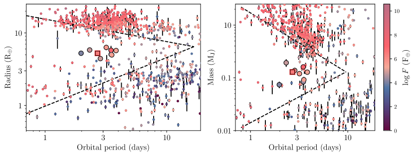
Figure 11: The hot Neptunian desert reported in Mazeh et al. (2016) shown as dashed lines. Planets (as of September 2022) from the TEPCat catalogue of "well-studied transiting planets" (Southworth, 2011, https://www.astro.keele.ac.uk/jkt/tepcat/allplanets-noerr.html) with uncertainties smaller than 30% in radius (left) and mass (right). The points are colour coded according to the incident flux, which is truncated at $F=1$ F_⊕. TOI-1288 b is shown as the large square with a red outline. The large circles denote the closest eight planets to TOI-1288 b in the radius-period parameter space, with their position highlighted in the mass-radius diagram as well.

What is clear from Fig. 11 is that the upper boundary is much more well-defined than the lower boundary. However, even if the lower boundary would be at larger radii, TOI-1288 b is still found in a very deserted area. In Fig. 11 we have highlighted eight planets that are the closest to TOI-1288 b in the radius-period (distance here measured in units of $(\mathrm{R}_{\oplus}^{2}+\mathrm{days}^{2})^{1/2}$) plane; Kepler-101 b (Bonomo et al., 2014), HATS-7 b (Bakos et al., 2015), TOI-532 b (Kanodia et al., 2021), TOI-674 b (Murgas et al., 2021), TOI-1728 b (Kanodia et al., 2020), NGTS-14Ab (Smith et al., 2021), WASP-156 b (Demangeon et al., 2018), and K2-55 b (Crossfield et al., 2016). Some key parameters (Southworth, 2011, from https://www.astro.keele.ac.uk/jkt/tepcat/allplanets-noerr.html) for these systems are summarised in Table 5 along our parameters for TOI-1288 b.

Obviously, the planets are similar in terms of period and radius, but they also have quite similar masses, and thus densities. The most striking difference in Fig. 11 is the insolation, which is dictated by the spectral type ($T_{\mathrm{eff}}$) of the stellar host. In this context it is worth noting that the overabundance of large planets with high insolation compared to at smaller radii in Fig. 11, merely reflects that it is easier to detect a larger planet around a larger (hotter) star. This is apparent from Fig. 17 and also what is seen in Szabó & Kálmán (2019).

A clustering of Neptune-sized planets with equilibrium temperatures of around 2000 K has been reported in Persson et al. (2022), which begs the question whether there could be an island of stability in the desert. However, this might also be a selection effect, and more planets in this parameter space are needed to establish this. It is an intriguing idea, and if an island of stability could exist for these slightly smaller planets on more irradiated orbits, maybe a similar island exist for TOI-1288 b and its neighbours, who are slightly bigger and less irradiated. It could also be a strip of pseudo stability in the desert, or it might just reflect the aforementioned less well-defined lower boundary of the desert.

Table 5: Closest radius-period neighbours. The eight planets closest to TOI-1288 b in terms of radius and period (with distance in units of $(\mathrm{R}_{\oplus}^{2}+\mathrm{days}^{2})^{1/2}$).

	$P$	$F$†	$R_{\rm p}$	$M_{\rm p}$	$\rho_{\rm p}$	SpT
	(d)	(F⊕)	(R⊕)	(M⊕)	($\rho_{\oplus}$)
TOI-1288 b	2.6998	630	5.6	41	0.24	G
TOI-532 b	2.327	119	5.8	61	0.31	M
TOI-674 b	1.977	57	5.3	24	0.17	M
Kepler-101 b	3.488	1260	5.8	51	0.26	G
HATS-7 b	3.185	288	6.3	38	0.15	K
TOI-1728 b	3.492	72	5.1	27	0.21	M
NGTS-14Ab	3.536	240	5.0	29	0.25	K
WASP-156 b	3.836	186	5.7	41	0.24	K
K2-55 b	2.849	130	4.4	44	0.5	K

• From $(\rho_{\star}/\rho_{\odot})^{-2/3}(P/1~{}\mathrm{yr})^{-4/3}(T_{\mathrm{eff}}/5777~{}\mathrm{K})^{4}$.

5.2 Internal structure and atmosphere

In the mass-radius diagram in Fig. 12 we compare TOI-1288 b to models with different compositions. The models are taken from Zeng et al. (2016, 2019). Evidently, TOI-1288 b can be described as a rocky core with a gaseous envelope at high irradiation. Probing the atmosphere of the planet through transmission spectroscopy could naturaully help reveal atmospheric features, but can also provide valuable constraints on the internal structure.

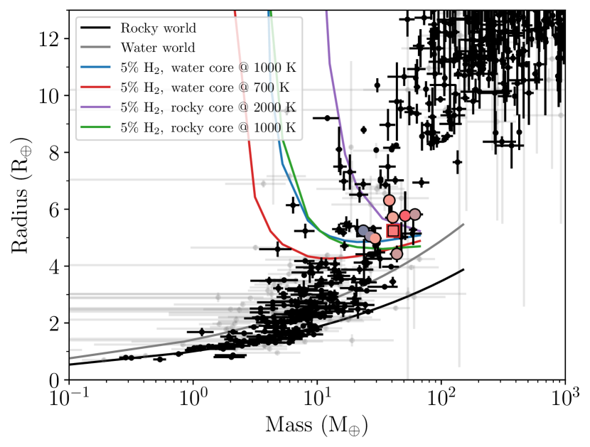
Figure 12: Mass-radius diagram. Planets from the same catalogue as in Fig. 11, but now for planets with uncertainties on both mass and radius of less (more) than 30% shown as black (grey) dots. Solid lines are composition models from Zeng et al. (2016, 2019). TOI-1288 b is again shown as the large (coloured) square with the similar ($R_{\mathrm{p}},P$) planets shown with large circles.

We observed a transit of planet b on the night 2020 June 11 using the HARPS-N spectrograph. The RVs from this night can be seen around orbital phase 0.0 in the lower left panel of Fig. 6, but due to the slow rotation of the star ($v\sin i_{\star}=1.3\pm 1.2$ km s^-1) we do not see the Rossiter-McLaughlin (RM; Rossiter, 1924; McLaughlin, 1924) effect. For an aligned configuration a decent approximation for the amplitude is given by $0.7\sqrt{1-b^{2}}(R_{\rm P}/R_{\star})^{2}v\sin i_{\star}$, which comes out to just shy of 2 m s^-1 for TOI-1288 b.

We nonetheless ran an MCMC where we included the RM effect (using the code by Hirano et al., 2011). We excluded the photometry and instead applied Gaussian priors to $P_{\rm b}$, $T_{\rm 0,b}$, $(R_{\rm p}/R_{\star})_{\rm b}$, $(a/R_{\star})_{\rm b}$, and $i_{\rm b}$ using the values in Table 4 and for $v\sin i_{\star}$ from the SME value in Table 3. We also applied Gaussian priors to the macro- and micro-turbulence as well as the sum of the limb-darkening coefficients (values estimated from Doyle et al., 2014; Bruntt et al., 2010; Claret & Bloemen, 2011, respectively), while applying a uniform prior to the sky-projected obliquity, $\lambda_{\rm b}$. The rest followed the same approach as the run in Section 3. The resulting value for the projected obliquity was $\lambda_{\rm b}=70^{+110}_{-100}$^∘, meaning that it is unconstrained.

Following Kempton et al. (2018) we can calculate the transmission spectroscopic metric (TSM) to assess the feasibility of transmission spectroscopy for TOI-1288 b. The TSM is given by

$$\mathrm{TSM}=H\times\frac{R_{\rm p}^{3}T_{\rm eq}}{M_{\rm p}R_{\star}^{2}}\times 10^{-m_{J}/5}\,,$$ (4)

where $m_{J}$ is the apparent magnitude of the host in the $J$ band and $H$ is a scale factor related to the size of the planet. For TOI-1288 b $H$ is 1.15, while the planet, stellar, and system parameters are listed in Table 4, Table 3 (SED), and Table 1, respectively. This yields a TSM of $\sim 87$, which is just below the suggested cutoff for follow-up efforts in Kempton et al. (2018).

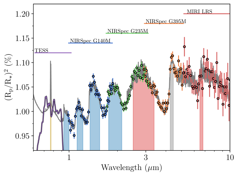
Figure 13: Simulated JWST observations. A simulated transmission spectrum of TOI-1288 b in grey using petitRADTRANS. The coloured error bars are simulated JWST data from PandExo of different instruments with their wavelength coverage shown by the horizontal coloured lines and with the names of the instrument shown above. We also show the TESS transmission curve in purple. Some atomic and molecular species are highlighted in the coloured areas with K, H₂O, CH₄, and CO₂ shown with yellow, blue, red, and grey, respectively.

While – according to this metric – TOI-1288 b is not a high priority target for JWST (Gardner et al., 2006), we still investigate what JWST might be able to detect if it were to do transmission spectroscopy. We simulated the spectrum of TOI-1288 b using petitRADTRANS (Mollière et al., 2019, 2020) assuming a cloud-free, isothermal model at 1266 K. We used PandExo (Batalha et al., 2017) to simulate the JWST data for four different instruments. For each we assumed a total of 4 transits with a 4 hr baseline each. The resulting spectrum is shown in Fig. 13. For this most likely quite optimistic scenario, JWST should be able to detect several molecular species, such as H₂O, CH₄, and CO₂ (if present).

5.3 Outer companions

According to the Web TESS Viewing Tool, TOI-1288 is (at the time of writing) being re-observed in Sectors 56-58 (beginning in September 2022 and ending in November 2022). These additional sectors should help refine the transit parameters of planet b. While our current estimate for the period and ephemeris of planet c suggest a transit occurred (of course, depending on the inclination) July 2022, the uncertainties are rather large, so it is worthwhile to be on the look out for a potential transit of planet c.

Zhu & Wu (2018) and Bryan et al. (2019) found an excess of cold Jupiters in systems harbouring super-Earths/sub-Neptunes with the former stating that stars with super-Earths have roughly a 3 times higher cold Jupiter fraction compared to field stars. Furthermore, they found that this cold Jupiter fraction rises to about 60% for stars with $\rm[Fe/H]>0.1$. Given the metallicity we find for TOI-1288 of $0.07\pm 0.09$ from the SED (median from all measurements in Table 3 is 0.15), it is perhaps not too surprising that we are seeing a cold gas giant in this system. This strong correlation between super-Earths and cold Jupiters suggests that they are not competing for the same solid material, which Zhu & Wu (2018) argue disfavours theories invoking large-scale migration.

On the other hand TOI-1288 b is a bit larger than the planets in the aforementioned studies and might have a gaseous envelope. In line with the discussion above, hot Neptunes are in danger of losing their atmospheres, especially while their stars are young and active (e.g. Lopez et al., 2012). Kozai-Lidov cycles and high-eccentricity migration can deliver Neptune-sized planets on short period orbits past this active stage ($\sim 100$ Myr) for the star (Dawson & Johnson, 2018). Interactions between TOI-1288 b and c could therefore be responsible for transporting TOI-1288 b to its current position. Subsequent tidal interactions with the star could then have dampened the eccentricity to the current value ($0.064^{+0.014}_{-0.015}$), which compared to Earth’s orbit ($\sim 0.016$) is still significant.

To assess whether planet c can influence the dynamics of the inner, planetary system as we see it today, we calculated the planet-star coupling parameter, $\epsilon_{\star 1}$, given in Lai et al. (2018), which is a measure for whether an outer companion can cause the orbit of the inner planet to precess. For this we used the approximation in their Eq. (24), which is made for the case of a hot Jupiter with a gas giant companion at a separation of around 1 AU. While not exactly the case here, the approximation can still provide us with some qualitative insights.

As we need to know the stellar rotation period, $P_{\rm rot}$, for this, we searched the TESS light curve using the autocorrelation method (McQuillan et al., 2013), however, we did not detect any signs of stellar rotation. Instead we estimated $P_{\rm rot}$ from the age, $\tau=10.05$ Gyr (Table 3), and colour, $B-V=0.94$ (Table 1), using the relation in Mamajek & Hillenbrand (2008), which yields a rotation period of 64 d. From this we get $\epsilon_{\star 1}\sim 0.5$ suggesting a strong coupling between TOI-1288 b and the star. However, it is not too far from the resonant regime of $\epsilon_{\star 1}\sim 1$, meaning the excitation of the spin-orbit angle, the obliquity, could be possible.

In addition to TOI-1288 c for which we have constrained the orbit and thus the mass to some extent, we also see evidence for what could be a companion on an even wider orbit. However, for the time being we can only make rather crude inferences about the characteristics of this companion as was done in Section 4, namely Fig. 10. For instance, if this companion were on a 10 yr coplanar (with respect to TOI-1288 b) orbit it would have a mass of around 0.3 M_J. To decipher the dynamic influence from this companion on the architecture would require continued RV monitoring to trace out the orbit.

6 Conclusions

Here we presented the discovery of multiple planets in the TOI-1288 system. Using photometry from TESS as well as ground-based telescopes, we have determined that the transiting planet TOI-1288 b is a super Neptune ($5.24\pm 0.09$ R_⊕) on a short period orbit ($2.699835^{+0.000004}_{-0.000003}$ d). TOI-1288 b thus joins the growing population of super Neptunes that despite the drought have settled in the Neptunian desert. We have characterised the planet in terms of mass through intensive RV monitoring with the HARPS-N and HIRES spectrographs, where we find a mass of $42\pm 3$ M_⊕.

Combining the radius and mass for TOI-1288 b, we find that the planet can be described as a rocky core with a gaseous envelope at high radiation. Similar compositions are found for the planets most identical to TOI-1288 b in terms of orbital period and radius, meaning that the internal structure and composition might be a crucial premise for survival in the desert. Atmospheric studies of occupants in and around the desert could help shed light on the processes, such as photoevaporation, shaping this region. TOI-1288 b is a well-suited candidate for such studies.

Furthermore, from our RV monitoring we also found evidence for an additional companion in the TOI-1288 system with an orbital period of $443^{+11}_{-13}$ d. We find a lower mass of $84\pm 7$ M_⊕, meaning that if this companion is close to being coplanar with TOI-1288 b, it would be a Saturn-mass planet. TOI-1288 c might have been responsible for transporting TOI-1288 b from a further out orbit to its present day location, for instance, through high-eccentricity migration. Finally, we detect hints of a long-term RV trend possibly caused by another body in the TOI-1288 system.

Data Availability

The radial velocities underlying this article are available in its online supplementary material.

Appendix A Figures

Figure 17: The hot Neptunian desert as in Fig. 11, but with the colour coding done in the host star effective temperature.

Appendix B Tables

Table 6: Ground-based photometry. Information on our ground-based photometric observations.

Observatory	Location	Aperture (m)	Photometric Aperture (arcsec)	UTC Date	Filter	Coverage
LCOGT1-TFN	Tenerife, Spain	1.0	5.8	2021-09-18	$z$-short2	Full
LCOGT-TFN	Tenerife, Spain	1.0	5.8	2021-09-18	$B$	Full
Whitin	Massachusetts, USA	0.7	8.0	2020-11-15	$z^{\prime}$	Full
Whitin	Massachusetts, USA	0.7	8.0	2020-11-15	$g^{\prime}$	Full
Ca l’Ou3	Catalonia, Spain	0.4	6.7	2021-05-14	$B$	Full
Albany$\rm\grave{a}$4	Catalonia, Spain	0.4	12.2	2019-12-02	$I_{\rm c}$	Full
MuSCAT5	Okayama, Japan	1.88	5.4	2019-10-31	Sloan $g^{\prime}$	Ingress
MuSCAT	Okayama, Japan	1.88	5.4	2019-10-31	Sloan $r^{\prime}$	Ingress
MuSCAT	Okayama, Japan	1.88	5.4	2019-10-31	$z$-short2	Ingress

• Las Cumbres Observatory Global Telescope (LCOGT; Brown et al., 2013).

• Pan-STARRS $z$-short.

• Observatori de Ca l’Ou, Sant Martí Sesgueioles.

• Albany$\rm\grave{a}$ Observatory.

• Multicolor Simultaneous Camera for studying Atmospheres of Transiting exoplanets (MuSCAT; Narita et al., 2015).

Table 7: Radial velocities. The epochs, RVs, and errors from the HARPS-N and HIRES observations. This table is available in its entirety online.

Epoch	RV	$\sigma_{\mathrm{RV}}$	Instrument
BJDTDB	m s-1	m s-1
2458790.340214	-68045.93	1.21	HARPS-N
2458790.359751	-68048.67	1.27	HARPS-N
2458821.330149	-68073.51	1.16	HARPS-N
⋮	⋮	⋮	⋮
2459702.697487	-68051.86	0.90	HARPS-N
2458827.739873	32.38	1.22	HIRES
2458844.755499	4.83	1.28	HIRES
2458852.719975	11.01	1.28	HIRES
⋮	⋮	⋮	⋮
2459498.888082	-14.75	1.51	HIRES

Table 8: Limb-darkening coefficients. The limb-darkening coefficients for our MCMC using a quadratic limb-darkening law. We stepped in the sum of the coefficients with a Gaussian prior ($\mathcal{N}(\mu,\sigma)$), while keeping the difference fixed ($\mathcal{F}(c)$). The initial values were found from the tables in Claret (2017) for the case of TESS and Claret & Bloemen (2011) for the rest of the filters.

Parameter	Name	Prior	Value
Stepping parameters
$\rm\delta M$	Dilution	$\mathcal{N}$(4.41,0.02)	$4.410^{+0.021}_{-0.019}$
$(q_{1}+q_{2})_{1}$	Sum of limb-darkening coefficients TESS	$\mathcal{N}$(0.6184,0.1)	$0.57\pm 0.05$
$(q_{1}+q_{2})_{1}$	Sum of limb-darkening coefficients TESS	$\mathcal{N}$(0.6184,0.1)	$0.57\pm 0.05$
$(q_{1}+q_{2})_{2}$	Sum of limb-darkening coefficients Albany$\rm\grave{a}$ $I$	$\mathcal{N}$(0.6611,0.1)	$0.67^{+0.10}_{-0.09}$
$(q_{1}+q_{2})_{3}$	Sum of limb-darkening coefficients Whitin $g^{\prime}$	$\mathcal{N}$(0.804,0.1)	$0.86^{+0.03}_{-0.07}$
$(q_{1}+q_{2})_{4}$	Sum of limb-darkening coefficients Whitin $z^{\prime}$	$\mathcal{N}$(0.5544,0.1)	$0.57\pm 0.10$
$(q_{1}+q_{2})_{5}$	Sum of limb-darkening coefficients LCO TFN $z$-short	$\mathcal{N}$(0.5544,0.1)	$0.53\pm 0.09$
$(q_{1}+q_{2})_{6}$	Sum of limb-darkening coefficients LCO TFN $B$	$\mathcal{N}$(0.8402,0.1)	$0.95^{+0.03}_{-0.05}$
$(q_{1}+q_{2})_{7}$	Sum of limb-darkening coefficients CALOU $B$	$\mathcal{N}$(0.8402,0.1)	$0.95^{+0.03}_{-0.05}$
$(q_{1}+q_{2})_{8}$	Sum of limb-darkening coefficients MuSCAT $g^{\prime}$	$\mathcal{N}$(0.804,0.1)	$0.87^{+0.03}_{-0.08}$
$(q_{1}+q_{2})_{9}$	Sum of limb-darkening coefficients MuSCAT $r^{\prime}$	$\mathcal{N}$(0.712,0.1)	$0.72\pm 0.10$
$(q_{1}+q_{2})_{10}$	Sum of limb-darkening coefficients MuSCAT $z$-short	$\mathcal{N}$(0.5544,0.1)	$0.56\pm 0.10$
Fixed parameters
$(q_{1}-q_{2})_{1}$	Difference of limb-darkening coefficients TESS	$\mathcal{F}(0.1598)$
$(q_{1}-q_{2})_{2}$	Difference of limb-darkening coefficients Albany$\rm\grave{a}$ $I$	$\mathcal{F}(0.2025)$
$(q_{1}-q_{2})_{3}$	Difference of limb-darkening coefficients Whitin $g^{\prime}$	$\mathcal{F}(0.79)$
$(q_{1}-q_{2})_{4}$	Difference of limb-darkening coefficients Whitin $z^{\prime}$	$\mathcal{F}(0.209)$
$(q_{1}-q_{2})_{5}$	Difference of limb-darkening coefficients LCO TFN $z$-short	$\mathcal{F}(0.209)$
$(q_{1}-q_{2})_{6}$	Difference of limb-darkening coefficients LCO TFN $B$	$\mathcal{F}(0.9002)$
$(q_{1}-q_{2})_{7}$	Difference of limb-darkening coefficients CALOU $B$	$\mathcal{F}(0.9002)$
$(q_{1}-q_{2})_{8}$	Difference of limb-darkening coefficients MuSCAT $g^{\prime}$	$\mathcal{F}(0.79)$
$(q_{1}-q_{2})_{9}$	Difference of limb-darkening coefficients MuSCAT $r^{\prime}$	$\mathcal{F}(0.4344)$
$(q_{1}-q_{2})_{10}$	Difference of limb-darkening coefficients MuSCAT $z$-short	$\mathcal{F}(0.209)$
Derived parameters
$(q_{1})_{1}$	Linear limb-darkening coefficient TESS		$0.36\pm 0.02$
$(q_{1})_{1}$	Quadratic limb-darkening coefficient TESS		$0.20\pm 0.02$
$(q_{1})_{2}$	Linear limb-darkening coefficient Albany$\rm\grave{a}$ $I$		$0.44\pm 0.05$
$(q_{2})_{2}$	Quadratic limb-darkening coefficient Albany$\rm\grave{a}$ $I$		$0.23\pm 0.05$
$(q_{1})_{3}$	Linear limb-darkening coefficient Whitin $g^{\prime}$		$0.824^{+0.016}_{-0.034}$
$(q_{2})_{3}$	Quadratic limb-darkening coefficient Whitin $g^{\prime}$		$0.034^{+0.016}_{-0.034}$
$(q_{1})_{4}$	Linear limb-darkening coefficient Whitin $z^{\prime}$		$0.39\pm 0.05$
$(q_{2})_{5}$	Quadratic limb-darkening coefficient Whitin $z^{\prime}$		$0.18\pm 0.05$
$(q_{1})_{5}$	Linear limb-darkening coefficient LCO TFN $z$-short		$0.37\pm 0.05$
$(q_{2})_{5}$	Quadratic limb-darkening coefficient LCO TFN $z$-short		$0.16\pm 0.05$
$(q_{1})_{6}$	Linear limb-darkening coefficient LCO TFN $B$		$0.926^{+0.014}_{-0.026}$
$(q_{2})_{6}$	Quadratic limb-darkening coefficient LCO TFN $B$		$0.026^{+0.014}_{-0.026}$
$(q_{1})_{7}$	Linear limb-darkening coefficient CALOU $B$		$0.927^{+0.014}_{-0.027}$
$(q_{2})_{7}$	Quadratic limb-darkening coefficient CALOU $B$		$0.027^{+0.014}_{-0.027}$
$(q_{1})_{8}$	Linear limb-darkening coefficient MuSCAT $g^{\prime}$		$0.828^{+0.017}_{-0.038}$
$(q_{2})_{8}$	Quadratic limb-darkening coefficient MuSCAT $g^{\prime}$		$0.038^{+0.017}_{-0.038}$
$(q_{1})_{9}$	Linear limb-darkening coefficient MuSCAT $r^{\prime}$		$0.57\pm 0.05$
$(q_{2})_{9}$	Quadratic limb-darkening coefficient MuSCAT $r^{\prime}$		$0.14\pm 0.05$
$(q_{1})_{10}$	Linear limb-darkening coefficient MuSCAT $z$-short		$0.38\pm 0.05$
$(q_{2})_{10}$	Quadratic limb-darkening coefficient MuSCAT $z$-short		$0.17\pm 0.05$

References

- Aguirre Børsen-Koch et al. (2022) Aguirre Børsen-Koch V., et al., 2022, MNRAS, 509, 4344
- Allard et al. (2012) Allard F., Homeier D., Freytag B., 2012, Philosophical Transactions of the Royal Society of London Series A, 370, 2765
- Anglada-Escudé & Butler (2012) Anglada-Escudé G., Butler R. P., 2012, ApJS, 200, 15
- Astropy Collaboration et al. (2013) Astropy Collaboration et al., 2013, A&A, 558, A33
- Astropy Collaboration et al. (2018) Astropy Collaboration et al., 2018, AJ, 156, 123
- Astropy Collaboration et al. (2022) Astropy Collaboration et al., 2022, ApJ, 935, 167
- Bakos et al. (2015) Bakos G. Á., et al., 2015, ApJ, 813, 111
- Batalha et al. (2017) Batalha N. E., et al., 2017, PASP, 129, 064501
- Boch & Fernique (2014) Boch T., Fernique P., 2014, in Manset N., Forshay P., eds, Astronomical Society of the Pacific Conference Series Vol. 485, Astronomical Data Analysis Software and Systems XXIII. p. 277
- Bonnarel et al. (2000) Bonnarel F., et al., 2000, A&AS, 143, 33
- Bonomo et al. (2014) Bonomo A. S., et al., 2014, A&A, 572, A2
- Borucki et al. (2010) Borucki W. J., et al., 2010, Science, 327, 977
- Brasseur et al. (2019) Brasseur C. E., Phillip C., Fleming S. W., Mullally S. E., White R. L., 2019, Astrocut: Tools for creating cutouts of TESS images, Astrophysics Source Code Library, record ascl:1905.007 (ascl:1905.007)
- Brown et al. (2013) Brown T. M., et al., 2013, Publications of the Astronomical Society of the Pacific, 125, 1031
- Bruntt et al. (2010) Bruntt H., et al., 2010, MNRAS, 405, 1907
- Bryan et al. (2019) Bryan M. L., Knutson H. A., Lee E. J., Fulton B. J., Batygin K., Ngo H., Meshkat T., 2019, AJ, 157, 52
- Buchhave et al. (2010) Buchhave L. A., et al., 2010, ApJ, 720, 1118
- Buchhave et al. (2012) Buchhave L. A., et al., 2012, Nature, 486, 375
- Buchhave et al. (2014) Buchhave L. A., et al., 2014, Nature, 509, 593
- Cabrera et al. (2012) Cabrera J., Csizmadia S., Erikson A., Rauer H., Kirste S., 2012, A&A, 548, A44
- Castelli & Kurucz (2004) Castelli F., Kurucz R. L., 2004, astro-ph/0405087,
- Choi et al. (2016) Choi J., Dotter A., Conroy C., Cantiello M., Paxton B., Johnson B. D., 2016, ApJ, 823, 102
- Ciardi et al. (2015) Ciardi D. R., Beichman C. A., Horch E. P., Howell S. B., 2015, ApJ, 805, 16
- Claret (2017) Claret A., 2017, A&A, 600, A30
- Claret & Bloemen (2011) Claret A., Bloemen S., 2011, A&A, 529, A75
- Collins (2019) Collins K., 2019, in American Astronomical Society Meeting Abstracts #233. p. 140.05
- Collins et al. (2017) Collins K. A., Kielkopf J. F., Stassun K. G., Hessman F. V., 2017, AJ, 153, 77
- Cosentino et al. (2012) Cosentino R., et al., 2012, in Ground-based and Airborne Instrumentation for Astronomy IV. p. 84461V, doi:10.1117/12.925738
- Crossfield et al. (2016) Crossfield I. J. M., et al., 2016, ApJS, 226, 7
- Cutri et al. (2003) Cutri R. M., et al., 2003, VizieR Online Data Catalog, p. II/246
- Dawson & Johnson (2018) Dawson R. I., Johnson J. A., 2018, ARA&A, 56, 175
- Demangeon et al. (2018) Demangeon O. D. S., et al., 2018, A&A, 610, A63
- Djupvik & Andersen (2010) Djupvik A. A., Andersen J., 2010, in Highlights of Spanish Astrophysics V. p. 211 (arXiv:0901.4015), doi:10.1007/978-3-642-11250-8_21
- Doyle et al. (2014) Doyle A. P., Davies G. R., Smalley B., Chaplin W. J., Elsworth Y., 2014, MNRAS, 444, 3592
- Foreman-Mackey et al. (2013) Foreman-Mackey D., Hogg D. W., Lang D., Goodman J., 2013, PASP, 125, 306
- Foreman-Mackey et al. (2017) Foreman-Mackey D., Agol E., Angus R., Ambikasaran S., 2017, ArXiv
- Frandsen & Lindberg (1999) Frandsen S., Lindberg B., 1999, in Karttunen H., Piirola V., eds, Astrophysics with the NOT. p. 71
- Fridlund et al. (2017) Fridlund M., et al., 2017, A&A, 604, A16
- Fukui et al. (2011) Fukui A., et al., 2011, PASJ, 63, 287