A Geometric Model for Polarization Imaging on Projective Cameras

Abstract

The vast majority of Shape-from-Polarization (SfP) methods work under the oversimplified assumption of using orthographic cameras. Indeed, it is still not well understood how to project the Stokes vectors when the incoming rays are not orthogonal to the image plane. We try to answer this question presenting a geometric model describing how a general projective camera captures the light polarization state. Based on the optical properties of a tilted polarizer, our model is implemented as a pre-processing operation acting on raw images, followed by a per-pixel rotation of the reconstructed normal field. In this way, all the existing SfP methods assuming orthographic cameras can behave like they were designed for projective ones. Moreover, our model is consistent with state-of-the-art forward and inverse renderers (like Mitsuba3 and ART), intrinsically enforces physical constraints among the captured channels, and handles demosaicing of DoFP sensors. Experiments on existing and new datasets demonstrate the accuracy of the model when applied to commercially available polarimetric cameras.

1 Introduction

When light reflects on a surface, its polarization changes according to well-established physical rules that describe such interaction. Among all the factors involved in the process, the surface properties and its orientation also determine the final polarization state of the captured beam. For this reason the literature counts several works aiming at recovering surface properties from images taken with a rotating linear polarizer in front of the camera [31, 2, 20].

Recently, the availability of Division-of-Focal-Plane (DoFP) cameras raised the interest of the Computer Vision community in polarization-related applications. In particular, light polarization is typically exploited to recover surface orientation in the so-called Shape from Polarization (SfP) applications. Such methods are designed to recover the 3D shape of acquired objects from a single view thanks to the information intrinsically encoded in the polarimetric images [20, 25, 4, 27]. Several approaches in the SfP domain combine polarimetric imaging with other cues coming from classical techniques such as stereo [13], multi-view [1, 10, 35, 7] or shading [22, 26]. Moreover, some works presented in the recent past propose data-driven approaches to perform shape from polarization [3, 19] exploiting specially-made datasets which involve the use of polarimetric cameras and 3D scanners capturing a wide range of subjects, from small objects to entire buildings. Other practical applications of polarimetric data involve pose estimation [11], material classification [28] and HDR reconstruction [32], while some methods propose to extend the dense SLAM system [33]. Finally, some works propose a recovery of both surface geometry and refractive index via multispectral polarimetric imaging [15].

Despite the undeniable contribution of these approaches in the present-day relevant literature, almost all of them rely on the quite unrealistic assumption of operating with an orthographic camera. Indeed, the basic equations often presented in such works are designed for a model where light rays hit the sensor perpendicularly: this is pointed out in some early papers such as [24, 23]. The majority of proposed approaches employ pinhole cameras, in which light beams hit the image plane with an angle that depends on the camera geometry. In practice, assuming an orthographic model while acquiring with a projective camera leads to non-negligible errors and deformations, especially when we are interested on areas near the image borders or if we have short focal lengths. The authors of [6, 19] highlight the described problem and try to formulate a solution for the perspective deformation and the representation of polarization data in non-orthographic imaging devices.

1.1 Related Works

In the literature we find an abundance of methods focusing on Shape from Polarization but very few works trying to understand how to deal with projective cameras. Indeed, we are concerned that almost all the methods assume (explicitly or even implicitly) to have an orthographic camera, without considering how much this assumption might affects the results. Only recently, two works addressed this problem by providing two different solutions. Chen et al. [6] gave the first purely geometric relationship between the polarization phase angle and the azimuth angle of the observed surface normal. Albeit interesting, the model has two limitations. First, it does not account for normal elevation so its applicability is limited to some specific contexts (i.e. single-view recovery of planar surfaces or multi-view estimation of normals). Second, it does not provide a direct description of how the full polarization state (i.e. the Stokes vector) is captured, but only how the Angle of Linear Polarization is affected by the ray direction. The second work, proposed by Lei et. al [19], is based on the observation that “the polarization representation is highly influenced by the viewing direction”. Their solution consists on a Convolutional Neural Network taking in input the captured image together of a viewing encoding providing cues to the camera intrinsic properties. Accuracy of the resulting normal maps are currently unmatched, but such data-driven approaches give no explicit information on how the model works internally. As often happens with pure learning-based solutions, the resulting model is a black-box which can hardly be generalized to different contexts.

1.2 Our contributions

In this paper we give the first complete mathematical description of how the scene polarization is captured with a projective camera. Our model is based on the optical properties of the tilted polarizer [17] and formulated by applying the algebra of Mueller matrices. In this respect, the main contribution of our work is that the analysis of what happens in a projective camera not based on pure empirical evidence (i.e. data-driven) but on the physical well-studied background of how light polarization is represented and transformed when interacting with the camera optical elements. In doing so, we show how some formulas commonly used in SfP simply derive by the application of particular Mueller matrices to the incoming Stokes vectors.

One of the key advantages of the resulting model is that it can be applied as a pre-processing on the acquired image and a post-processing of the estimated normal field. Therefore, it can be used seamlessly on existing SfP methods designed with the orthographic assumption in mind. We adopted the same conventions assumed in popular direct and inverse renderers believing that this will simplify the creation of synthetic datasets closely simulating what can be captured with a real polarimetric camera. This topic is of a pivotal importance to train state-of-the-art deep learning based models and for testing existing methods against a controllable Ground Truth. Finally, the model is equally valid for DoFP and Division-of-Time (DoT) cameras, and generalizes to any number of linear polarizers involved in the acquisition process.

2 Preliminaries

To understand the theoretical background of the proposed model, we briefly summarize some basic notions about light polarization. The goal here is to highlight crucial aspects that are sometimes neglected when approaching shape-from-polarization. Please refer to [8, 5] to learn more about these concepts.

2.1 Light polarization

Any visible light ray consists of two orthogonal electric field components $E_{x},E_{y}$ oscillating in the plane transverse to the direction of propagation $\vec{k}$. Without loss of generality, $\vec{k}$ can be set coincident with the $z$-axis, so that $E_{x},E_{y},z$ form an orthogonal reference system in which:

$$E_{x}(z,t) = A_{x}\cos\big{(}\omega t-\frac{2\pi}{\lambda}z+\delta_{x}\big{)}$$

$$E_{y}(z,t) = A_{y}\cos\big{(}\omega t-\frac{2\pi}{\lambda}z+\delta_{y}\big{)}.$$ (1)

$A_{x}$ and $A_{y}$ are two wave amplitudes, $\omega$ is the angular frequency, $\lambda$ is the wavelength and $\delta_{x},\delta_{y}$ are two arbitrary phases. The point $\begin{pmatrix}E_{x}(z,t)&E_{y}(z,t)\end{pmatrix}$ traces a so called polarization ellipse when discarding the time-space propagator $\omega t-\frac{2\pi}{\lambda}z$ (i.e. when observing the two waves “projected” in the $x-y$ plane). Orientation angle and eccentricity of such ellipse describe the polarization state of light. For example, when $A_{y}=0,A_{x}>0$ the optical field oscillates horizontally and we have a linearly horizontal polarized light (polarization ellipse degenerates to an horizontal segment). When $A_{x}=A_{y},\delta_{x}-\delta_{y}=0$ we have polarized light with an Angle of Linear Polarization (AoLP) of $45^{\circ}$.

An important thing has to be noted here. When we discuss about polarization angles (horizontal, $45^{\circ}$, etc.) we have to make clear the orthogonal reference system in which the electric field components are expressed. The third axis is implicitly known, since we always assume the $z$-axis being the direction of propagation. The $x$-axis can be any unitary vector orthogonal to $z$, thus providing a reference to which such angles are expressed. Since the system is orthogonal, the $y$-axis is uniquely determined as $y=x\times z$. Therefore, a light ray with an AoLP of $45^{\circ}$ can be seen as a ray with an AoLP of $0^{\circ}$ if we rotate the reference system $45^{\circ}$ counter-clockwise around the $z$-axis.

2.2 Stokes parameters and Mueller matrices

$E_{x},E_{y}$ are not directly measurable, so a different formulation is usually preferred. Taking a time average of Eqs. 2.1 yield the definition of the four quantities:

$$S_{0} = A_{x}^{2}+A_{y}^{2}$$

$$S_{1} = A_{x}^{2}-A_{y}^{2}$$

$$S_{2} = 2A_{x}A_{y}\cos(\delta_{y}-\delta_{x})$$

$$S_{3} = 2A_{x}A_{y}\sin(\delta_{y}-\delta_{x})$$ (2)

called Stokes polarization parameters, usually grouped in the Stokes vector $S=\begin{pmatrix}S_{0}&S_{1}&S_{2}&S_{3}\end{pmatrix}^{T}$. This formulation is powerful because can describe partially polarized light as a mixture of unpolarized and completely polarized light:

$$S=(1-\rho)\begin{pmatrix}S_{0}\\ 0\\ 0\\ 0\end{pmatrix}+\rho\begin{pmatrix}S_{0}\\ S_{1}\\ S_{2}\\ S_{3}\end{pmatrix}$$ (3)

where $\rho=\sqrt{S_{1}+S_{2}+S_{3}}/S_{0}$ is called Degree of Linear Polarization (DoLP). It is easy to observe from Eq.3 that $S_{0}$ is the intensity of light and the AoLP $\phi$ is given by $\phi=\mbox{atan2}(S_{2},S_{1})$.

Stokes parameters can be measured by letting the light rays pass trough special materials called polarizers and retarders. Such elements transform the input Stoke vector by means of a linear transformation described by a $4\times 4$ Mueller matrix $\mathbf{M}$. For example, the Mueller matrix of an ideal linear polarizer with transmission axis oriented with an angle $\alpha$ with respect to the $x$-axis is:

$$\mathbf{M_{\alpha}}=\frac{1}{2}\begin{pmatrix}1&\cos 2\alpha&\sin 2\alpha&0\\ \cos 2\alpha&\cos^{2}2\alpha&\sin 2\alpha\cos 2\alpha&0\\ \sin 2\alpha&\sin 2\alpha\cos 2\alpha&\sin^{2}2\alpha&0\\ 0&0&0&0\end{pmatrix}.$$ (4)

Also in this case, the reference frame matters and cannot be chosen arbitrarily. The Mueller matrix of a polarizing element must be defined in a system coincident to the one in which the input/output Stokes vectors are expressed. If that’s not the case, a rotator $R$ (around the $z$-axis) must be applied to align the reference systems, thus getting:

$$S^{\prime}=R^{T}\mathbf{M}RS$$

where $S$ and $S^{\prime}$ are input and output Stokes vectors respectively. In any case, the $z$-axis of $S,S^{\prime}$ and $\mathbf{M}$ is fixed to the direction in which the ray travels. We stress the fact that Stokes vectors and Muller matrices alone are meaningless without an associated reference frame.

2.3 Polarimetric cameras

A polarimetric camera can measure the first $3$ components of a Stokes vector using an array of linear polarizers placed in front of a standard CCD or CMOS sensor. This can be implemented by adding fixed filters directly onto the pixel-grid (DoFP cameras), or by taking multiple pictures while rotating a linear polarizer in front of the lenses (DoT cameras). In both the cases, the polarizers are parallel to the image plane so that the transmitting axis is a vector $\vec{t}_{\alpha}=\begin{pmatrix}\cos\alpha&\sin\alpha&0\end{pmatrix}^{T}$ expressed in the camera reference frame.

Regardless the intrinsic properties of the camera (Orthographic or Projective), for each pixel a set of $\mathcal{I}=\{I_{\alpha_{0}},I_{\alpha_{1}},\ldots,I_{\alpha_{N}}\}$ intensities are captured by using linear polarizers with angles $\mathcal{A}=\{\alpha_{0},\alpha_{1},\ldots\alpha_{N}\}$ respectively. The task is to recover the incoming Stokes vector $S=\begin{pmatrix}S_{0}&S_{1}&S_{2}&0\end{pmatrix}^{T}$ from those observations.

2.4 Orthographic model

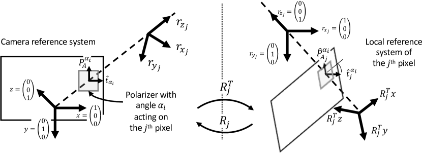
Figure 1: Sketch of the proposed model. In the camera reference system (left), the ray passing through the $j^{th}$ pixel (dashed line) is not propagating parallel to the $z$-axis. Therefore, the effect of a polarizer with angle $\alpha_{i}$ placed parallel to the image plane cannot be described with formulas used for orthographic cameras. To solve this, we define a local reference system for each ray (right) oriented along the direction of propagation. Since the linear polarizer is tilted, its effective angle $\hat{\alpha}_{i}^{j}$ is different from the actual orientation it has on the sensor. The tilted polarizer model [17] is used to compensate this distortion and recover the correct Stokes vector $S_{j}$ in the reference frame of the $j^{th}$ pixel. Finally, a rotation $R_{j}$ allow us to map normal vectors estimated from $S_{j}$ back to the camera reference system.

The orthographic camera model is simple to deal with because all the rays are assumed to enter perpendicularly to the image plane. Therefore, we can conveniently set the reference frame of all the rays such that the first two axes follows the horizontal and vertical ordering of the pixels, and the $z$-axis coincides with the camera optical axis (i.e. the direction in which all the rays are propagating). Note that, since the $y$-axis is commonly oriented downward (following the top-down ordering of image pixels) and the $x$-axes rightward, the polarization angles are measured clockwise from the $x$-axis instead of the classical counter-clockwise notation. So, care must be taken when using formulas involving polarization angles.

Since $S_{0}$ represents the light intensity, for each pixel we can easily relate the intensities $\mathcal{I}$ to the incoming Stokes vector $S$ by writing a set of linear equations:

$$\begin{pmatrix}I_{\alpha_{0}}\\ I_{\alpha_{1}}\\ \vdots\\ I_{\alpha_{N}}\end{pmatrix}=\begin{pmatrix}\mathbf{M}_{\alpha_{0}}^{1}\\ \mathbf{M}_{\alpha_{1}}^{1}\\ \vdots\\ \mathbf{M}_{\alpha_{N}}^{1}\end{pmatrix}\begin{pmatrix}S_{0}\\ S_{1}\\ S_{2}\\ 0\end{pmatrix}$$ (5)

where $\mathbf{M}_{\alpha_{i}}^{1}$ is the first row of the matrix $\mathbf{M}_{\alpha_{i}}$ (defined in Eq. 4). At this point, $S$ can be estimated by solving Eq. 5 in a least-squares sense [21, 14], usually by first expressing each equation $I_{\alpha_{i}}=\mathbf{M}_{\alpha_{i}}^{1}S$ in terms of AoLP $\phi$ and DoLP $\rho$:

$$I_{\alpha_{i}} = \frac{I_{\max}+I_{\min}}{2}+\frac{I_{\max}-I_{\min}}{2}\cos(2\alpha_{i}-2\phi)$$

$$\rho = \frac{I_{\max}-I_{\min}}{I_{\max}+I_{\min}}.$$ (6)

A special case is given by PFA cameras composed by just four polarizers arranged with angles $\alpha_{0,1,2,3}=0^{\circ},45^{\circ},90^{\circ},135^{\circ}$. In this setting, the trigonometric Eqs.  2.4 have a simple closed-form solution:

$$S_{0} = I_{0}+I_{90}$$

$$S_{1} = I_{0}-I_{90}$$

$$S_{2} = I_{45}-I_{135}.$$ (7)

Note that, for the orthogonality of such polarizers, intensities are subject to the constraint $I_{0}+I_{90}=I_{45}+I_{135}$. So, $S_{0}$ can alternatively be computed as $I_{45}+I_{135}$.

2.5 The proposed model

The problem of dealing with a projective camera arise because rays propagate in different directions and none of them, except the central one, is parallel to the optical axis. Therefore, we need to:

1. Define a reference system unique for each ray. The $z$-axis must always point to the direction of propagation but we still have freedom of choice for the other two. (Sec. 2.6)

2. Understand what happens to the Stokes vector when a ray traverse a linear polarizer tilted with respect to the ray direction (Sec. 2.7)

2.6 Local ray reference system

We suppose to know the matrix $\mathbf{K}$ of intrinsic camera parameters that can be estimated with any popular calibration tool. For each pixel $p_{j}=\begin{pmatrix}u_{j}&v_{j}\end{pmatrix}$ in the image plane, the corresponding exiting ray is the 3D unitary vector:

$$\vec{r}_{z_{j}}=\frac{\mathbf{K}^{-1}\begin{pmatrix}u_{j}&v_{j}&1\end{pmatrix}^{T}}{\|\mathbf{K}^{-1}\begin{pmatrix}u_{j}&v_{j}&1\end{pmatrix}^{T}\|}.$$ (8)

The third axis of $p_{j}$’s local reference system must be $\vec{r}_{z_{j}}$ because it represents its direction of propagation. For the other two axes we have freedom of choice. Without loss of generality, we set:

$$\vec{r}_{x_{j}} = \frac{\begin{pmatrix}0&1&0\end{pmatrix}^{T}\times\vec{r}_{z_{j}}}{\|\begin{pmatrix}0&1&0\end{pmatrix}^{T}\times\vec{r}_{z_{j}}\|}$$ (9)

$$\vec{r}_{y_{j}} = \vec{r}_{z_{j}}\times\vec{r}_{x_{j}}$$ (10)

thus creating the orthogonal reference system $\mathcal{P}_{j}=(\vec{r}_{x_{j}},\vec{r}_{y_{j}},\vec{r}_{z_{j}})$ shown in Fig. 1. Note that there is no physical reason to prefer $\vec{r}_{x_{j}}$ as defined in Eq. 9 since any other vector orthogonal to $\vec{r}_{z_{j}}$ would have been equally valid for the model. However, it makes sense to set the frame such that its horizontal axis is aligned with the camera $x$-axis (indeed, $r_{x_{j}}\perp y$ by construction). Moreover, this is the same convention used by the state-of-the-art polarization aware renderers Mitsuba [16] and ARC [30] so synthetically generated images can be easily compared with real images processed with our model. Finally, we define the matrix:

$$R_{j}=\begin{pmatrix}|&|&|\\ \vec{r}_{x_{j}}&\vec{r}_{y_{j}}&\vec{r}_{z_{j}}\\ |&|&|\end{pmatrix}$$ (11)

mapping vectors from $\mathcal{P}_{j}$ to the camera reference system.

2.7 Tilted polarizers

Polarimetric cameras are constructed so that the array of polarizers are parallel to the image plane. Therefore, in each local reference system $\mathcal{P}_{j}$, such polarizers are tilted and the transmission axis is in general not orthogonal to $\vec{r}_{z_{j}}$. For this reason, Eq. 5 is not correctly defined because each $\mathbf{M}_{\alpha_{i}}$ lie in the camera reference frame which is not aligned with the ray direction of propagation.

To solve the problem, we follow the empirical model of Korger et al.[17] assuming to have polarizing elements made of anisotropic absorbing and scattering particles. According to such model, the effective transmitting axis $\mathbf{\hat{t}}_{j}$ of a tilted polarizer is orthogonal to both $\vec{r}_{z_{j}}$ and the absorbing axis $\hat{P_{A}}_{j}$. In other words, the effect of a tilted polarizer with angle $\alpha$ is equivalent of a linear polarizer aligned with the ray direction (so that its effect on the Stokes vector can it be expressed with a Mueller matrix) but with a different effective angle $\hat{\alpha}$.

We can obtain the Mueller matrix $\mathbf{M}_{\hat{\alpha}_{i}^{j}}$ of the $i^{th}$ tilted polarizer on in the local frame of the $j^{th}$ pixel by computing the effective angle $\hat{\alpha}_{i}^{j}$ as follows:

$$\hat{P}_{A_{j}}^{\alpha_{i}} = R_{j}^{T}\begin{pmatrix}\cos(\alpha_{i}+\pi/2)\\ \sin(\alpha_{i}+\pi/2)\\ 0\end{pmatrix}$$ (12)

$$\mathbf{\hat{t}}_{j}^{\alpha_{i}} = \begin{pmatrix}\cos\hat{\alpha}_{i}^{j}\\ \sin\hat{\alpha}_{i}^{j}\\ 0\end{pmatrix}=\frac{\begin{pmatrix}0&0&1\end{pmatrix}^{T}\times\hat{P}_{A_{j}}^{\alpha_{i}}}{\|\begin{pmatrix}0&0&1\end{pmatrix}^{T}\times\hat{P}_{A_{j}}^{\alpha_{i}}\|}.$$ (13)

Equation 12 expresses the absorbing axis of the $i^{th}$ polarizer in the local reference frame of the ray. We add $\frac{\pi}{2}$ to the polarizer angle $\alpha_{i}$ because we assume the absorbing axis being orthogonal to the transmission axis. Then, Eq. 13 computes the effective transmitting axis $\mathbf{\hat{t}}_{j}^{\alpha_{i}}$, which is orthogonal to the ray direction of propagation by construction. The angle of $\mathbf{\hat{t}}_{j}^{\alpha_{i}}$ in the local reference frame of the ray gives the effective angle $\hat{\alpha}_{i}^{j}$.

To summarize, a perspective camera can be used like an orthographic one with the following precautions:

1. Each recovered Stokes vector is defined on a different reference frame, depending to the ray direction for that pixel. Consequently, normal vectors computed from the Stokes lie on different frames as well, and must be transformed back to the camera reference frame through $R_{j}$.

2. Even if the camera uses a few different polarizers with angles in $\mathcal{A}$, each pixel will observe equivalent polarizers with a different set of angles $\hat{\mathcal{A}}_{j}=\{\hat{\alpha}_{1}^{j},\hat{\alpha}_{2}^{j},\ldots,\hat{\alpha}_{N}^{j}\}$. This implies that a linear system like the one shown in Eq. 5 must be solved in any case, since simpler closed form solutions (See Eq. 7) cannot be valid simultaneously for all the pixels.

2.8 How to use our model

The main advantage our model is that it does not require to reformulate existing SfP methods designed with the orthographic camera assumption. Indeed, we can synthetize new images that would have been seen with ideal (non tilted) polarizers rotated at angles $0^{\circ},45^{\circ},90^{\circ},135^{\circ}$. After this pre-processing, Eq. 7 can be used get the full Stokes vector, AoLP and DoLP needed to compute the normal vector field. When normals are recovered, they will be expressed in the local reference frame of each pixel. So, every vector must be transformed to the common camera reference frame by applying the rotation $R_{j}$ (Eq. 11). This is a post-processing operation that can be transparently applied to the output of any SfP method. We now sketch the basic steps to be performed to embed our model in existing or future approaches for Shape-from-Polarization:

1. Calibrate the camera to get the intrinsic matrix $\mathbf{K}$

2. Compute per-pixel reference systems and transformation matrices $R_{j}$ using Eq. 11

3. For each pixel $j$ and for each polarizer angle $\alpha_{i}$, compute the effective polarizer angle $\hat{\alpha}_{i}^{j}$ using Eq. 13

4. Solve the linear system in Eq. 5 but using $\mathbf{M}_{\hat{\alpha}_{i}^{j}}^{1}$ instead of $\mathbf{M}_{\alpha_{i}}^{1}$ to compensate the effect of the tilted polarizers. This will produce a Stokes vector $S_{j}$ for each pixel. Note that this vector is not expressed in the camera reference frame but in the local pixel reference frame $\mathcal{P}_{j}$.

5. If the SfP method directly accepts the Stokes vector, use the ones computed in the previous step. Otherwise, pre-process the data by synthetizing a new set of images $\hat{\mathcal{I}}=\{\hat{I}_{0},\hat{I}_{45},\hat{I}_{90},\hat{I}_{135}\}$ where the image $\hat{I}_{\gamma}$ is obtained by multiplying each Stokes vector $S_{j}$ with the Muller matrix $\mathbf{M}_{\gamma}$.

6. Since Stokes vector are in local frames, the 3D normal vectors obtained by SfP are expressed in the local reference frames as well. Therefore, whenever a normal $\vec{n}_{j}$ is estimated for a pixel $j$, it must be transformed back to the camera reference system by computing $R_{j}\vec{n}_{j}$. This is essentially a post-processing operation to be applied to the resulting normal field.

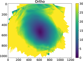
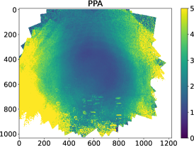
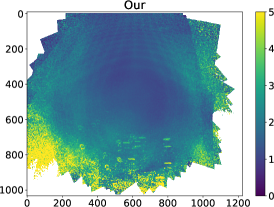
Figure 2: Average per-pixel error in degrees of the produced AoLP for three models. Note that the color bar for the Orthographic model is substantially different to avoid saturation.

Solving a small linear system for each pixel (Step 4) is the price to pay to compensate the effects of tilted polarizers. However, this operation can be used to seamlessly demosaic a DoFP camera. Indeed, in such cameras each pixel can only observe a single polarizer angle $\alpha_{i}$ similar to how a pixel observes a specific color in color cameras with Bayer pattern. Eq. 5 can be slightly adapted to accept groups of $H\times H$ neighbours of the $j^{th}$ pixel to produce $S_{j}$. The approach is similar to [34] but can now take into account the effective angles of the micro polarizers. Moreover, the synthetized images produced in the Step 5 satisfy physical constraints deriving from the orthogonality of the polarizers. Indeed, it is guaranteed that $\hat{I}_{0}+\hat{I}_{90}=\hat{I}_{45}+\hat{I}_{135}$ which was not true in general for raw images in $\mathcal{I}$ regardless the effect of the tilted polarizers. This problem was rarely addressed in the literature but can introduce biases in the computation of Stokes vector since we implicitly give more importance to some polarizer angles ($0$ and $90$ degrees) with respect to the other pair. With our approach this problem disappears and corrections like the one proposed in [12] are no longer required.

3 Experiments

In this section we present some experiments to evaluate the ability of the proposed model to accurately describe how the Stokes vector are imaged by a projective camera. The two other similar methods available in the literature are the well known Orthographic model and the recent Perspective Phase Angle (PPA) proposed by Chen et. al.[6]. As discussed before, we recall that PPA just relates the AoLP $\phi$ of the light to the surface normal without giving a unified description of what happens to the whole Stokes vector. Therefore, comparisons against PPA is limited to specific experiments discussed in Secs. 3.1 and 3.2. To reduce uncertainty due to uncontrollable scene conditions (mixed polarization, accuracy of the Ground Truth surface normals, $\frac{\pi}{2}$-ambiguity, etc.) we follow the approach of [6] that uses a glossy planar plastic board with markers attached to it. In this way, the orientation of the plane (i.e. its normal in camera reference frame) can be accurately recovered. We created from scratch a new dataset similar to the PPA dataset provided in [6] but using a different camera and lenses. Specifically, we used a FLIR Blackfly camera mounting a $5$ Mpixel Sony IMX250MZR DoFP sensor with $8$mm lenses. Scene was illuminated with sunlight in a very overcast day so that the DoLP of incoming light is close to $0$. The resulting dataset is composed by $360$ images of the glossy plane taken at different angles and distances. Both PPA and our datasets are used for evaluation.

3.1 AoLP recovery

	PPA Dataset		Our Dataset
	MAE	RMSE	MAE	RMSE
Ortho	$13.60\pm 8.66$	$16.13$	$7.66\pm 9.48$	$9.50$
PPA [6]	$1.95\pm 1.56$	$2.52$	$4.89\pm 6.43$	$6.50$
Our	$\mathbf{1.54}\pm\mathbf{1.39}$	$\mathbf{2.10}$	$\mathbf{4.68}\pm\mathbf{6.27}$	$\mathbf{6.25}$

Table 1: MAE and RMSE of the AoLP produced with the three compared models from the GT normal vectors of the plane. Values are in degrees.

We started by measuring the agreement between the AoLP $\phi_{c}$ captured by the camera and the expected AoLP $\phi_{m}$ computed by the three models (Ortho, PPA, and Our). In the Orthographic model $\phi_{m}=\mbox{atan2}(n_{y},n_{x})$ (i.e. the AoLP is equal to the azimuth angle of the surface normal $\vec{n}=(n_{x},n_{y},n_{z})^{T}$), in PPA is given by Eq. 6 in [6], and in our model is computed like the Orthographic model but with the pre/post-processing explained in Sec. 2.8. We manually checked that specular reflection is dominant in both the PPA and our dataset, so the $\pi$-ambiguity is the only one that can happen on the AoLP. Therefore, in computing the errors we take the best between $\phi_{m}$ and $\phi_{m}+\pi$.

Results are listed in Tab. 1. Both PPA and our model return a significantly lower error than the Orthographic model. This result, consistent to what declared in [6], should raise the awareness that ignoring the perspective distortion is probably not reasonable for accurate Shape-from-polarization. Our model performs better in both the datasets because it compensates the effect of tilted polarizers. Both the MAE and RMSE of our model shows an impovement of $\approx 25\%$ wrt. PPA. In Fig. 2 we show the per-pixel Mean Absolute Error (MAE) when computing the AoLP on the whole PPA dataset. Not considering some small artefacts at the bottom due to specular highlights that saturate some pixels, we observe a strong radial pattern in the Orthographic MAE (left-most image). This is expected, since rays corresponding to pixels farther away to the principal point are more tilted than the ones closer to it. In our model this effect is strongly attenuated, showing evidence that the perspective distortion have been effectively compensated. PPA performs better than Ortho, but the radial pattern is still partially visible.

3.2 Plane orientation estimation

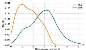
Figure 3: Plane normal error distributions for our method and PPA.

	PPA Dataset		Our Dataset
	MAE	RMSE	MAE	RMSE
Orthographic	$13.441\pm 6.653$	$14.997$	$10.546\pm 5.467$	$11.879$
Our	$1.923\pm 1.343$	$2.346$	$4.373\pm 2.935$	$5.267$
Smith	$28.494\pm 12.379$	$31.067$	$34.848\pm 5.477$	$35.275$
Smith corrected	$27.396\pm 12.489$	$31.021$	$33.870\pm 6.399$	$34.470$
SfPW CNN	$38.305\pm 22.915$	$44.637$	$22.819\pm 15.649$	$27.670$

Table 2: Comparison of normal estimation errors on PPA and our plane datasets between different SfP methods. Projective (Our) and Orthographic methods use an oracle to solve all the ambiguities. Errors are in degrees.

Since in the Orthographic model $\phi$ is the azimuth angle of $\vec{n}$, the linear constraint

$$\begin{pmatrix}\sin\phi&\cos\phi&0\end{pmatrix}\cdot\vec{n}=0$$ (14)

is usually considered in photo-polarimetric stereo approaches or iso-depth contour tracing. If we know that at least $K>3$ pixels observe the same plane, we can use such constraint to recover the plane normal $\vec{n}$ (in camera reference frame) from the (corrected) $\phi_{j}$ observed at each pixel by solving:

$$\begin{pmatrix}\begin{pmatrix}\sin\phi_{1}&\cos\phi_{1}&0\end{pmatrix}R_{1}^{T}\\ \begin{pmatrix}\sin\phi_{2}&\cos\phi_{2}&0\end{pmatrix}R_{2}^{T}\\ \vdots\\ \begin{pmatrix}\sin\phi_{K}&\cos\phi_{K}&0\end{pmatrix}R_{K}^{T}\\ \end{pmatrix}\vec{n}=\vec{0}$$ (15)

as a Linear Least-Squares problem. Note that the system is under-determined in the Orthographic model because all the rays are parallel ($R_{1},\ldots R_{k}$ are identities) and all the pixels would observe the same $\phi$. In the PPA model, instead, a similar costraint is provided (See Eq. 7 in [6]).

In Fig. 3 we plotted the the estimated plane normal error distribution against the Ground Truth data in the PPA dataset. The Ortho model is not present in the plot for the reasons discussed before. Also in this case, our mean absolute error is lower ($1.57^{\circ}$ vs. $2.89^{\circ}$) and with less variability. This reflects a better estimation of the AoLP due to the correction applied by the tilted polarizer model.

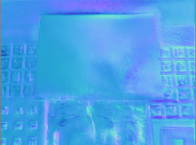
Figure 4: Qualitative comparison of the estimated normal field with methods Ortho (left), Our (center), and SfPW (right) on an instance of the PPA dataset. Errors are computed only inside the plane area but we kept the rest of the scene for visualization purposes. Note how a radial pattern is visible in the Ortho model since the distortion due to the ray orientation is not accounted for. SfPw performs poorly because it has been trained on a much noisier dataset and apparently is not able to generalize to simpler scenarios.

3.3 Normal estimation

Our work is not a SfP method, so evaluating its validity based on how well a normal field is reconstructed has to be done with care. We recall that the azimuth angle of $\vec{n}$ is equal to the AoLP $\phi$ up to a (unavoidable) $\pi$-ambiguity, and an additional $\frac{\pi}{2}$-ambiguity depending if specular or diffuse reflection dominates. Since in the plane dataset the specular reflection is dominant, we used the following function to relate the DoLP $\rho$ with zenith angle $\theta$ and the index of refraction $n$ :

$$\rho(n,\theta)=a\frac{2\sin^{2}\theta\cos\theta\sqrt{n^{2}-\sin^{2}\theta}}{n^{2}-\sin^{2}\theta-n^{2}\sin^{2}\theta+2\sin^{4}\theta}$$ (16)

where $a$ is a scale parameter we added to the original formulation shown in [2] to account for a possible diffuse component of reflection and other nonlinear contribution like the Umov’s effect [18, 29].

To show the validity of our approach, the idea is to test how well our model allows the recovery of surface normals in ideal conditions, i.e. with an oracle that removes the ambiguities and provides a close estimate of the unknown parameters $n,a$ in Eq. 16. Since we know the Ground Truth normals of both the datasets, we manually estimated the best value of the two parameters and computed the errors considering the minimum error among all the possible ambiguities. We compare the resulting normal field against: (i) the orthographic model using the same oracle as our method (i.e. estimated function $\rho$ and optimal disambiguator); (ii) Smith et al. [26]; (iii) Smith corrected with our pre/post processing to account for projective camera, and (iv) SfPW [19], a Deep CNN with a multi-head self-attention module and viewing encoding “to account for non-orthographic projection in scene-level”. We used the original author implementation pre-trained on their SPW Dataset.

We listed the MAE and RMSE of the estimated normals in Tab. 2. Normals recovered with our projective model are significantly more accurate than the others. This is not surprising, since we assume to have an oracle that resolves all the unknowns we usually face when doing SfP. The important thing to notice here is the improvement against the orthographic model that uses the same oracle. In other words, properly accounting for non orthographic projection is crucial to reduce the error, no matter how sophisticated is the method applied to solve the ambiguities. Moreover, the Smith corrected performs better than the original one because can now accounts for non-orthographic cameras. We stress that this correction was performed as pre/post processing without modifying any other part of the method. Finally, SfPW performs well but not better than the “simple” Orthographic model. Considering that SfPW can take into account non-orthographic cameras, we expected a lower error in this experiment. In general, SfP is difficult to solve without posing additional strong priors to the reconstructed scene, and learning-based method can only try to resolve the ambiguities based on what observed on the training set, with the risk of overfitting specific 3D structures. In Fig. 4 we show a qualitative example of the obtained normal field.

3.4 Other datasets

We also tested our method on a dataset of general objects presented in [3]. In this case it is difficult to provide an oracle because it contains scenes with different kind (diffuse/specular) and degrees of polarization. So, we limit our test to the observation of how the pre/post processing can improve an existing SfP method. Similarly to what we did with planes dataset, we compare Smith, Smith corrected, SfPW and DeepSfP[3]. The latter method is a Deep model assuming an orthographic camera, so potentially is a valid candidate to be corrected with our model. However, at the time of writing, the code and pre-trained weights were not publicly available so we report here the results shown in the original paper. Tab. 3 show the MAE of the estimated normals in the whole dataset. SfPW is the best performing method, followed by DeepSfP. It is interesting to observe that, also in this case, Smith corrected with our model obtains a significant improvement.

	MAE (deg)
Smith	$45.39$
Smith corrected	$32.52$
SfPW CNN	$14.68$
DeepSfP	$18.52$

Table 3: Normal estimation errors on DeepSfP dataset

4 Conclusions

We presented a model to describe how a projective camera captures the light polarization state. Differently than the empirical PPA model [6], our formulation derives by the optical properties of the tilted polarizer and the algebra of Mueller matrices. We consider it as a unifying model, equally valid to DoFP and ToFP cameras (i.e. with polarizers above the sensor or in front of the lenses) and consistent with conventions used by polarization-aware renderers. It allows to embed demosaicing of DoFP cameras directly in the Stokes estimation and, finally, can be implemented by means of a pre-processing of acquired raw data and post-processing of the reconstructed surface normals. In the experimental section we observed a good agreement between the obtained Stokes vector (in terms of AoLP and DoLP linked to the surface normals) and the expected one deriving by the geometry of some controlled planar scenes. For the future, we aim to generalize our model to include lens distortion, vignetting on acquired DoLP due to the Umov’s effect, and noise deriving by cross-talking between pixels.

References

- [1] Gary A Atkinson and Edwin R Hancock. Multi-view surface reconstruction using polarization. In ICCV, volume 2, page 3, 2005.
- [2] Gary A Atkinson and Edwin R Hancock. Recovery of surface orientation from diffuse polarization. IEEE transactions on image processing, 15(6):1653–1664, 2006.
- [3] Yunhao Ba, Alex Gilbert, Franklin Wang, Jinfa Yang, Rui Chen, Yiqin Wang, Lei Yan, Boxin Shi, and Achuta Kadambi. Deep shape from polarization. In European Conference on Computer Vision, pages 554–571. Springer, 2020.
- [4] Seung-Hwan Baek, Daniel S Jeon, Xin Tong, and Min H Kim. Simultaneous acquisition of polarimetric svbrdf and normals. ACM Trans. Graph., 37(6):268–1, 2018.
- [5] M. Bass, C. DeCusatis, J.M. Enoch, V. Lakshminarayanan, G. Li, C. MacDonald, V.N. Mahajan, and E. Van Stryland. Handbook of Optics, Third Edition Volume I: Geometrical and Physical Optics, Polarized Light, Components and Instruments(set). Handbook of Optics. McGraw Hill LLC, 2009.
- [6] Guangcheng Chen, Li He, Yisheng Guan, and Hong Zhang. Perspective phase angle model for polarimetric 3d reconstruction. arXiv preprint arXiv:2207.09629, 2022.
- [7] Lixiong Chen, Yinqiang Zheng, Art Subpa-Asa, and Imari Sato. Polarimetric three-view geometry. In Proceedings of the European Conference on Computer Vision (ECCV), pages 20–36, 2018.
- [8] E. Collett. Field Guide to Polarization. Field Guide Series. SPIE Press, 2005.
- [9] Thomas W Cronin and Justin Marshall. Patterns and properties of polarized light in air and water. Philosophical Transactions of the Royal Society B: Biological Sciences, 366(1565):619–626, 2011.
- [10] Zhaopeng Cui, Jinwei Gu, Boxin Shi, Ping Tan, and Jan Kautz. Polarimetric multi-view stereo. In Proceedings of the IEEE conference on computer vision and pattern recognition, pages 1558–1567, 2017.
- [11] Zhaopeng Cui, Viktor Larsson, and Marc Pollefeys. Polarimetric relative pose estimation. In Proceedings of the IEEE/CVF International Conference on Computer Vision, pages 2671–2680, 2019.
- [12] Tehreem Fatima, Mara Pistellato, Andrea Torsello, and Filippo Bergamasco. One-shot hdr imaging via stereo pfa cameras. In International Conference on Image Analysis and Processing, pages 467–478. Springer, 2022.
- [13] Yoshiki Fukao, Ryo Kawahara, Shohei Nobuhara, and Ko Nishino. Polarimetric normal stereo. In Proceedings of the IEEE/CVF Conference on Computer Vision and Pattern Recognition, pages 682–690, 2021.
- [14] Cong Phuoc Huynh, Antonio Robles-Kelly, and Edwin Hancock. Shape and refractive index recovery from single-view polarisation images. In 2010 IEEE Computer Society Conference on Computer Vision and Pattern Recognition, pages 1229–1236. IEEE, 2010.
- [15] Cong Phuoc Huynh, Antonio Robles-Kelly, and Edwin R Hancock. Shape and refractive index from single-view spectro-polarimetric images. International journal of computer vision, 101(1):64–94, 2013.
- [16] Wenzel Jakob, Sébastien Speierer, Nicolas Roussel, Merlin Nimier-David, Delio Vicini, Tizian Zeltner, Baptiste Nicolet, Miguel Crespo, Vincent Leroy, and Ziyi Zhang. Mitsuba 3 renderer, 2022. https://mitsuba-renderer.org.
- [17] Jan Korger, Tobias Kolb, Peter Banzer, Andrea Aiello, Christoffer Wittmann, Christoph Marquardt, and Gerd Leuchs. The polarization properties of a tilted polarizer. Optics express, 21(22):27032–27042, 2013.
- [18] Meredith K Kupinski, Christine L Bradley, David J Diner, Feng Xu, and Russell A Chipman. Angle of linear polarization images of outdoor scenes. Optical Engineering, 58(8):082419, 2019.
- [19] Chenyang Lei, Chenyang Qi, Jiaxin Xie, Na Fan, Vladlen Koltun, and Qifeng Chen. Shape from polarization for complex scenes in the wild. In Proceedings of the IEEE/CVF Conference on Computer Vision and Pattern Recognition, pages 12632–12641, 2022.
- [20] Daisuke Miyazaki, Robby T Tan, Kenji Hara, and Katsushi Ikeuchi. Polarization-based inverse rendering from a single view. In Computer Vision, IEEE International Conference on, volume 3, pages 982–982. IEEE Computer Society, 2003.
- [21] Shree K Nayar, Xi-Sheng Fang, and Terrance Boult. Separation of reflection components using color and polarization. International Journal of Computer Vision, 21(3):163–186, 1997.
- [22] Trung Ngo Thanh, Hajime Nagahara, and Rin-ichiro Taniguchi. Shape and light directions from shading and polarization. In Proceedings of the IEEE conference on computer vision and pattern recognition, pages 2310–2318, 2015.
- [23] Stefan Rahmann. Polarization images: a geometric interpretation for shape analysis. In Proceedings 15th International Conference on Pattern Recognition. ICPR-2000, volume 3, pages 538–542. IEEE, 2000.
- [24] Stefan Rahmann and Nikos Canterakis. Reconstruction of specular surfaces using polarization imaging. In Proceedings of the 2001 IEEE Computer Society Conference on Computer Vision and Pattern Recognition. CVPR 2001, volume 1, pages I–I. IEEE, 2001.
- [25] Moein Shakeri, Shing Yang Loo, Hong Zhang, and Kangkang Hu. Polarimetric monocular dense mapping using relative deep depth prior. IEEE Robotics and Automation Letters, 6(3):4512–4519, 2021.
- [26] William AP Smith, Ravi Ramamoorthi, and Silvia Tozza. Height-from-polarisation with unknown lighting or albedo. IEEE transactions on pattern analysis and machine intelligence, 41(12):2875–2888, 2018.
- [27] Vage Taamazyan, Achuta Kadambi, and Ramesh Raskar. Shape from mixed polarization. arXiv preprint arXiv:1605.02066, 2016.
- [28] Shoji Tominaga and Akira Kimachi. Polarization imaging for material classification. Optical Engineering, 47(12):123201, 2008.
- [29] von N Umow. Chromatische depolarisation durch lichtzerstreuung. Phys. Z, 6:674–676, 1905.
- [30] Alexander Wilkie. The advanced rendering toolkit, 2018. http://cgg.mff.cuni.cz/ART.
- [31] Lawrence B Wolff and Terrance E Boult. Constraining object features using a polarization reflectance model. Phys. Based Vis. Princ. Pract. Radiom, 1:167, 1993.
- [32] Xuesong Wu, Hong Zhang, Xiaoping Hu, Moein Shakeri, Chen Fan, and Juiwen Ting. Hdr reconstruction based on the polarization camera. IEEE Robotics and Automation Letters, 5(4):5113–5119, 2020.
- [33] Luwei Yang, Feitong Tan, Ao Li, Zhaopeng Cui, Yasutaka Furukawa, and Ping Tan. Polarimetric dense monocular slam. In Proceedings of the IEEE conference on computer vision and pattern recognition, pages 3857–3866, 2018.
- [34] Junchao Zhang, Haibo Luo, Bin Hui, and Zheng Chang. Image interpolation for division of focal plane polarimeters with intensity correlation. Optics express, 24(18):20799–20807, 2016.
- [35] Jinyu Zhao, Yusuke Monno, and Masatoshi Okutomi. Polarimetric multi-view inverse rendering. In European Conference on Computer Vision, pages 85–102. Springer, 2020.