RSD measurements from BOSS galaxy power spectrum using the halo perturbation theory model

Abstract

We present growth of structure constraints from the cosmological analysis of the power spectrum multipoles of SDSS-III BOSS DR12 galaxies. We use the galaxy power spectrum model of [1], which decomposes the galaxies into halo mass bins, each of which is modeled separately using the relations between halo biases and halo mass. The model combines Eulerian perturbation theory and halo model calibrated on $N$-body simulations to model the halo clustering. In this work, we also generate the covariance matrix by combining the analytic disconnected part with the empirical connected part: we smooth the connected component by selecting a few principal components and show that it achieves good agreement with the mock covariance. Our analysis differs from recent analyses in that we constrain a single parameter $f\sigma_{8}$ fixing everything else to Planck+BAO prior, thereby reducing the effects of prior volume and mismodeling. We find tight constraints on $f\sigma_{8}$: $f\sigma_{8}(z_{\mathrm{eff}}=0.38)=0.489\pm 0.038$ and $f\sigma_{8}(z_{\mathrm{eff}}=0.61)=0.455\pm 0.028$ at $k_{\mathrm{max}}=0.2\ h$Mpc^-1, with an overall amplitude error of 5%, and in good agreement (within 0.3 sigma) of Planck amplitude. We discuss the sensitivity of cosmological parameter estimation to the choice of scale cuts, covariance matrix, and the inclusion of hexadecapole $P_{4}(k)$. We show that with $k_{\mathrm{max}}=0.4\ h$Mpc^-1 the constraints improve considerably to an overall 3.2% amplitude error, but there is some evidence of model misspecification on MultiDark-PATCHY mocks. Choosing $k_{\mathrm{max}}$ consistently and reliably remains the main challenge of RSD analysis methods.

1 Introduction

Large-scale clustering of the galaxies in redshift surveys is one of the major cosmological probes which gives us insight into gravity, dark energy, and primordial non-Gaussianities. We can quantify this structure using the 2-point correlation function or the power spectrum. The 2-point analyses have made accurate measurements of baryon acoustic oscillations (BAO), caused by sound waves in the pre-decoupling Universe [2]. The BAO data have both isotropic and anisotropic components, and with galaxy samples from Baryon Oscillation Spectroscopic Survey (BOSS), a part of Sloan Digital Sky Survey (SDSS)-III, it provides constraints on the distance scale with a percent-level precision [3].

Galaxy clustering amplitude cannot be directly related to the dark matter amplitude due to galaxy biasing. However, we can consider another kind of anisotropy in the clustering of galaxies caused by the redshift-space distortions (RSD). It is created by peculiar velocities of galaxies, affecting the measured clustering signal in redshift space along the line-of-sight, but not transverse to it. Such distortions depend on the underlying matter density field, which are correlated with the velocity field. In the linear regime we parametrize RSD with the parameter $\beta=f/b$, where $f$ is the linear growth rate, and $b$ is the galaxy bias [4]. On small scales the linear theory breaks down, and non-linear distortions, such as the Finger-of-God (FoG) effect, clustering dilution in redshift space along the line of sight due to the motion of galaxies within virialized dark matter halos, need to be accounted for.

RSD has become one of the most powerful cosmological probes by measuring the growth of structure via the parameter combination $f(z)\sigma_{8}(z)$, thereby testing dark energy and different gravity models. [5] provides the 2.5% constraint on $f\sigma_{8}$ on the BOSS CMASS galaxies using a simulation-based analysis, but [5] does not employ an analytic approach to model the small-scale clustering and uses only a single simulation box. [3] presents the Data Release 12 (DR12) final consensus results on the BOSS galaxies, over the redshift range $0.2<z<0.75$, and provides 9.3 and 8.0% $f\sigma_{8}$ constraints on low-redshift ($z_{\mathrm{eff}}=0.38$) and high-redshift galaxies ($z_{\mathrm{eff}}=0.61$). More recently, there are BOSS DR12 measurements of the growth of structure from PT-based models [6, 7, 8, 9] and from simulation-based models [10, 11, 12, 13]. In particular, [12] proposes a Gaussian Process emulator and provides 7.4, 5.6, and 4.9% constraints on $f\sigma_{8}$ at $z_{\mathrm{eff}}=0.25,0.4$ and $0.55$, and [13] develops a hybrid emulator which combines emulator with Markov chain Monte Carlo (MCMC) sampling, giving the 3.6% constraint on the BOSS CMASS galaxies. In addition, some of the recent works measure the clustering of the DR16 extended BOSS (eBOSS) samples and provides the growth of structure measurements [14, 15].

This work applies the redshift-space galaxy power spectrum model of [1] to the BOSS DR12 galaxy samples. [1] proposes an approach which combines perturbation theory(PT)-based modeling techniques and simulation-based analyses. Following the halo model formalism in [16], this model decomposes a galaxy sample into centrals and satellites and separately model the 1-halo and 2-halo—correlations of 2 galaxies in the same and different halos, respectively—contributions to the clustering of galaxies. The dark matter halo power spectrum model in redshift space is based on the distribution function approach [17, 18, 19, 20, 21, 22], and Eulerian PT and halo biasing model are used to model the underlying dark matter correlator terms [21]. Then, some of the key terms in the models are calibrated from the results of N-body simulations. [1] tests and validates this power spectrum model by performing independent tests using high-fidelity, periodic $N$-body simulations and realistic BOSS CMASS mocks, showing that the recovered values of $f\sigma_{8}$ has only small bias.

In this work, we not only extend the work from [1] by applying its power spectrum model to the BOSS DR12 galaxies but also develop the hybrid covariance matrix, which combines the analytic disconnected part [23] and empirical connected part, including up to four principal components. Such covariance matrix can be especially useful for the analysis of next-generation redshift surveys. We also discuss how the choice of scale cuts, covariance matrix, and the inclusion of hexadecapole $P_{4}(k)$ affect our clustering analysis and show that removing BAO information from the multipole measurements only affects cosmological parameter estimation in a negligible way. We also compare our growth of structure constraints with other BOSS DR12 measurements in the literature, based on both PT-based models and simulation-based models.

In this paper we adopt a different approach than many of the recent papers [3, 6, 9, 11, 7, 13, 10, 12] in that we only fit a single parameter $f\sigma_{8}$ to the RSD data, fixing everything else. There are several reasons for this approach. First of all, angular clustering in linear regime of redshift space is directly probing $f\sigma_{8}$, and it is reasonable to analyze the parameter that is closest to the data. Many of recent analyses of BOSS data find a low amplitude compared to Planck (see e.g. Fig. 9), but the comparison is not straight-forward since they typically fit several parameters at once. Fitting several parameters to RSD data raises several issues: as the data are not sensitive to all of the parameters the priors become important, and these may bias the posteriors of parameters the data are sensitive to.

Second issue has to do with model misspecification. All of the RSD models are likely misspecified to some extent: there are significant biases in parameter fits already at $k=0.2$h/Mpc [24], which is the scale typically adopted in the data analysis, so there is model misspecification already at that scale. Since RSD is strongly correlated with AP parameter [25] $F_{AP}(z)=D_{A}(z)H(z)(1+z)$, where $D_{A}$ is angular diameter distance, $H(z)$ is Hubble parameter and $z$ is the redshift, this problem can be exacerbated, since even a small model misspecification can lead to a large bias in the parameter fits due to this correlation: this is seen in the fits to the model used in this paper [1], where the bias of free AP parameter can be larger than the bias of fixed AP parameter. For this reason fixing AP parameter may be less prone to bias in the parameter fits. Furthermore, AP parameter is well measured by Planck+BAO (or by BBN+BAO). Indeed, $\lim_{z=0}[F_{AP}/z]\equiv 1$ by definition, so at low redshifts there is no point in fitting for $F_{AP}$ at all. For CMASS and Lowz data used in this paper the uncertainty in $F_{AP}$ from Planck+BAO [26] is very small compared to the precision of AP parameter we can achieve from RSD: $F_{AP}(z=0.38)=0.584\pm 0.001$ and $F_{AP}(z=0.61)=1.18\pm 0.003$. For this reason we fix $F_{AP}$ to Planck+BAO value. We have verified that varying $F_{AP}$ within Planck+BAO uncertainties makes no effect on the derived $f\sigma_{8}$ value.

A third issue is that we want to compare RSD analysis to Planck, but if we fit several parameters we must compare all of them, and account for multiple comparisons by the appropriate Look Elsewhere factor. However, RSD is really sensitive to $f\sigma_{8}$ parameter only, which argues for doing a single parameter analysis and compare its value to Planck. Our primary motivation is to compare BOSS RSD analysis to Planck, rather than to other RSD analyses which have adopted a different methodology. We want to phrase the comparison as one of (dis)agreement between Planck and BOSS RSD, and for this reason we simply fix everything except the parameter that BOSS RSD is most sensitive to.

The remainder of this paper is organized as follows. In section 2, we describe the mock simulations used to validate our model and the actual galaxy sample from BOSS DR12 used for the main analysis. Section 3 presents the galaxy power spectrum estimator and model parameters, as well as the survey window function convolved with the model. In section 4, we outline analysis methods for the cosmological parameter estimation and introduce the hybrid covariance matrix, demonstrating its accuracy compared to the mock covariance matrix. In section 5, we validate the model performance by providing test results on the mock catalogues which mimic the BOSS DR12 target selection. In section 6, we discuss the main results of this paper and conclude in section 7.

2 Data

2.1 SDSS-III BOSS DR12

In this work, we use the spectroscopic galaxy samples from SDSS-III BOSS DR12 [27, 28, 29, 30, 31, 32], selected using the imaging data from earlier SDSS-I and SDSS-II surveys. The BOSS DR12 samples are divided into the three redshift bins - z1 ($0.2<z<0.5$), z2 ($0.4<z<0.6$), and and z3 ($0.5<z<0.75$), following [3]. Because z2 overlaps with the other two samples and thus gives results correlated with others, we only consider z1 and z3, two non-overlapping BOSS DR12 samples. Each sample is observed in two different patches on the sky: North Galactic Cap (NGC) and South Galactic Cap (SGC). The BOSS DR12 sample, covering the redshift range $0.2<z<0.75$ over the area of 10,252 deg², contains 1,198,006 galaxies - 864,924 in NGC and 333,082 in SGC, and due to the difference in the imaging of the NGC and SGC samples, they have different characteristics, such as the bias parameter, and therefore we run an independent analysis on each sky region.

To address the problems arising from incompleteness of the BOSS survey, we apply weights to the galaxies, where the weights are given by

$$w=w_{\mathrm{sys}}(w_{\mathrm{no-z}}+w_{\mathrm{cp}}-1),$$ (2.1)

where $w_{\mathrm{sys}}$ is a systematic weight. $w_{no-z}$ and $w_{\mathrm{cp}}$ correct for missing redshifts due to failure to obtain redshift (no-z) and fiber collisions for close pairs (cp) [33].

The effective redshift for the z1 and z3 samples can be obtained as

$$z_{\mathrm{eff}}=\frac{\sum_{i}^{N_{\mathrm{gal}}}w_{\mathrm{fkp},i}\cdot w_{i}\cdot z_{i}}{\sum_{i}^{N_{\mathrm{gal}}}w_{\mathrm{fkp},i}\cdot w_{i}},$$ (2.2)

where $w_{\mathrm{fkp}}=(1+\bar{n}(z)P_{0})^{-1}$ with $P_{0}=10^{4}h^{-3}$Mpc³. We find that $z_{\mathrm{eff}}=0.38$ and 0.61, respectively for z1 and z3.

2.2 MultiDark-PATCHY mock catalogues

We use the MultiDark(MD)-PATCHY mock catalogues [34] for the BOSS DR12 dataset, produced using approximate gravity solvers and galaxy biasing models calibrated to the BigMultiDark simulations, which use $3840^{3}$ particles on a volume of $(2.5h^{-1}Mpc)^{3}$, and it reproduces the observed evolution of the clustering of the BOSS DR12. All quantities in these catalogues assume Planck13 cosmology: $\Omega_{m}=0.307115,\Omega_{L}=0.692885,\Omega_{b}=0.048,\sigma_{8}=0.8288$ and $h=0.6777$. We have 2048 mock catalogues available for both NGC and SGC hemispheres.

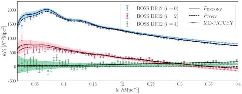
In section 4.1.1, we use Version 6C (V6C) catalogues, which is adjusted to reproduce the observed clustering measurements of the BOSS DR12, to evaluate the mock covariance matrix. Figure 2 shows that the power spectrum multipoles of V6C catalogues (colored dotted curves) match well with the BOSS DR12 measurements (circular data points). In section 3.1, we use Version 6S (V6S) catalogues to confirm that our theoretical model is accurate enough to obtain the cosmological parameter constraints. However, the difference between V6C and V6S catalogues are only subtle [35].

3 Redshift-space galaxy power spectrum

3.1 Model: perturbation theory

In this work, we use the galaxy power spectrum model of [1], which is based on perturbation theory combined with simulation-based calibration of halo model terms. We only briefly summarize the model here and refer the reader to [1] for more details.

This model follows the halo model formalism in [16], separately modeling the 1-halo and 2-halo contributions to the correlation of central and satellite galaxies. For this modeling, we decompose the galaxy sample into four sub-samples, based on whether there exists at least one other neighboring satellite in the given halo: isolated centrals without satellites (“type A” centrals), centrals with one or more satellites (“type B” centrals), isolated satellites (“type A” satellites), and non-isolated satellites (“type B” satellites). Such sub-sampling helps us separate 1-halo and 2-halo terms when modeling the total galaxy power spectrum in redshift space:

$$P_{gg}(\mathbb{k})=(1-f_{s})^{2}P_{cc}(\mathbb{k})+2f_{s}(1-f_{s})P_{cs}(\mathbb{k})+f_{s}^{2}P_{ss}(\mathbb{k}),$$ (3.1)

where $P^{cc},P^{cs}$, and $P^{ss}$ are the auto-power spectrum of centrals, the central-satellite cross-power spectrum, and the auto-power spectrum of satellites, respectively, and $f_{s}$ is the satellite fraction. We also account for non-linear distortions caused by the large virial motions of satellite galaxies within their halos - known as the Finger-of-God effect. We model this effect with a Lorentzian damping factor $G(k\mu;\sigma_{v})=(1+k^{2}\mu^{2}\sigma_{v}^{2}/2)^{-2}$ applied to the redshift-space power spectrum of each sub-sample, where $\sigma_{v}$ is the velocity dispersion of the sample. In this model, we assume a single velocity dispersion parameter for both type A and type B centrals, $\sigma_{c}$, and parameters for type A satellites, $\sigma_{s_{A}}$, and for type B satellites, $\sigma_{s_{B}}$. We take $\sigma_{c}$ and $\sigma_{s_{A}}$ as free parameters and determine $\sigma_{s_{B}}$ from the relation between the linear bias and velocity dispersion, using the relation for the halo mass and bias and the virial theorem scaling between velocity dispersion and mass.

The resulting galaxy power spectrum model depends on the following 11 physically-motivated parameters:

$$[f(z_{\mathrm{eff}}),\sigma_{8}(z_{\mathrm{eff}}),b_{1,c_{A}},b_{1,s_{A}},b_{1,s_{B}},f_{s},f_{s_{B}},\langle N_{>1,s}\rangle,\sigma_{c},\sigma_{s_{A}},f^{1h}_{s_{B}s_{B}}].$$

This includes two cosmological parameters, the growth rate $f$ and the amplitude of matter fluctuations $\sigma_{8}$ evaluated at the effective redshift of the sample $z_{\mathrm{eff}}$, and linear bias parameters of type A centrals and type A and B satellites ($b_{1,c_{A}}$, $b_{1,s_{A}}$, $b_{1,s_{B}}$). We also consider the fraction of all satellites $f_{s}$, the fraction of type B satellites $f_{s_{B}}$, and the mean number of satellite galaxies in halos with more than one satellite $\langle N_{>1,s}\rangle$. The velocity dispersion parameters for some sub-samples ($\sigma_{c}$ and $\sigma_{s_{A}}$) are accounted for, and we also vary the normalization nuisance parameter for the 1-halo amplitude $f^{1h}_{s_{B}s_{B}}$. Additionally, there exists the Alcock-Paczynski (AP) effect, geometric distortions of the galaxy statistics due to the mismatch between the true cosmology and the fiducial cosmology which we assumed when converting redshifts and angular positions of the observed galaxies into the three-dimensional physical positions. The AP parameter is very insensitive to cosmological parameters [36, 37]. As a result we fix the scaling factors $\alpha_{\parallel}$ and $\alpha_{\perp}$ of the AP effect to their fiducial values of Planck cosmology. We have verified that varying $F_{AP}$ within its error from Planck+BAO has negligible effect on the final constraints. The primary goal of this paper is to determine the growth rate $f\sigma_{8}$, and we will not attempt to separate $\sigma_{8}$ from $f$.

Since we only wish to determine one parameter $f\sigma_{8}$, the question remains whether fixing other parameters that modify the shape of the power spectrum has an impact on its value or its error. We have tested this by performing the full analysis of a set of 30 power spectra drawn at random from Planck+BAO chains. We find a scatter in $f\sigma_{8}$ best fit value at the level of roughly 30% of the statistical error. When combining errors in quadrature this leads to an additional 5% increase in statistical error, which we include in the final results.

3.2 Measurement: power spectrum estimator

We measure the galaxy clustering signal via the multipole moments of the power spectrum $P_{l}(k)$, using nbodykit, the python software package for large-scale structure data analysis. In nbodykit, the FFT-based algorithm for the anisotropic power spectrum estimator, presented in [38], is implemented. This provides fast evaluation of the estimator in [39] by expanding the Legendre polynomials into spherical harmonics rather than using a Cartesian decomposition and thereby requiring only $2l+1$ FFTs to obtain a multipole of order $l$.

We estimate the power spectrum multipoles as:

$$P_{l}(k)=\frac{2l+1}{A}\int\frac{d\Omega_{k}}{4\pi}F_{0}(\mathbb{k})F_{l}(\mathbb{-k}),$$ (3.2)

where $\Omega_{k}$ is the solid angle in Fourier space, and $\mathcal{L}_{l}$ is the Legendre polynomial. $A$ is the normalization defined as $A\equiv\int d\mathbb{r}[n^{\prime}_{\mathrm{gal}}(\mathbb{r})w_{\mathrm{fkp}}(\mathbb{r})]^{2}$, where $n^{\prime}_{\mathrm{gal}}$ is the weighted galaxy number density field, and $w_{\mathrm{fkp}}$ is the FKP weight.

The weighted galaxy density field $F(\mathbb{r})$ is given by

$$F(\mathbb{r})=\frac{w_{\mathrm{fkp}}(\mathbb{r})}{A^{1/2}}[n^{\prime}_{\mathrm{gal}}(\mathbb{r})-\alpha^{\prime}n^{\prime}_{\mathrm{ran}}(\mathbb{r})],$$ (3.3)

where $n^{\prime}_{\mathrm{gal}}$ and $n^{\prime}_{\mathrm{ran}}$ are the number density field for the galaxy and randoms catalogues respectively, with the factor $\alpha^{\prime}$ normalizing $n^{\prime}_{\mathrm{ran}}$ to $n^{\prime}_{\mathrm{gal}}$, and

$$\begin{split}F_{l}(\mathbb{k})&=\int d\mathbb{r}F(\mathbb{r})e^{i\mathbb{k}\cdot\mathbb{r}}\mathcal{L}_{l}(\mathbb{\hat{k}}\cdot\mathbb{\hat{r}})\\ &=\frac{4\pi}{2l+1}\sum_{m=-l}^{l}Y_{lm}(\mathbb{\hat{k}})\int d\mathbb{r}F(\mathbb{r})Y_{lm}^{*}(\mathbb{\hat{r}})e^{i\mathbb{k}\cdot\mathbb{r}}.\end{split}$$ (3.4)

We compute each summation over $m$ using a FFT, hence a total of $2l+1$ FFTs.

Figure 1: The window function multipoles in configuration space for the BOSS DR12 z1 (Left) and z3 (Right) samples. We include up to $Q_{8}(s)$ because the contribution of $l=10$ or higher is negligible for the window convolution.

However, [40] replaces the traditional definition of the normalization term $A$ with the value enforcing the following condition on the window function multipole of order $l=0$, $Q_{0}(s\rightarrow 0)=1$, to ensure that the power spectrum and window function are normalized in a consistent way. Table 1 in [40] shows that such correction of the normalization term results in increasing the BOSS DR12 galaxy power spectrum multipole amplitudes by roughly 10%. Following [40], we corrected all galaxy power spectrum measurements presented in this work.

3.3 Survey window function

We account for the window function effects by convolving the theoretical model in section 3.1 with the survey window function, which corresponds to the Fourier transform of the survey volume. We denote the resulting quantity as the “convolved” power spectrum.

Figure 2: The window function effects on the power spectrum multipoles (filled circles with error bars) for the BOSS DR12 z3 NGC sample. The solid and dashed curves correspond to the unconvolved and convolved multipoles, respectively. We also show the mean of 1000 MD-PATCHY V6C mock catalogues (colored dotted curves), and shaded areas indicate 1$\sigma$ deviations of 1000 mocks. Dotted curves match well with the data points, suggesting that V6C catalogues reproduce the clustering of the observed data (which makes them suitable for the covariance matrix estimation). For our main analysis, we choose the minimum wavenumber of $k_{\mathrm{min}}=0.02h$Mpc^-1 to minimize any large-scale effects of the window function.

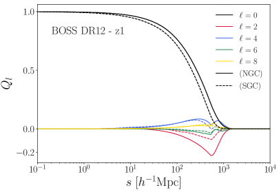
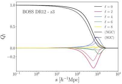
We follow the method presented in [41] to compute the convolved power spectrum multipoles. First, we use the pair counting algorithm in nbodykit [42], which employs the Corrfunc package [43], to obtain the pair counts of the random catalogue. In figure 1, we present the resulting window function multipoles, $Q_{l}(s)\propto\int_{-1}^{1}d\mu RR(s,\mu)\mathcal{L}_{l}(\mu)\approx\sum_{i}RR(s_{i},\mu_{i})\mathcal{L}_{l}(\mu_{i})$, of the BOSS DR12 galaxy samples in configuration space, for a set of separations $s$. The z1 and z3 window function multipoles vanish on scales larger than $\approx$ 2000 and 3000 $h^{-1}$Mpc, respectively, and these correspond to the largest scales in the volume of the BOSS galaxy samples. In this work, we ignore $l=10$ or higher, as its contribution to the convolution is negligible.

Next, we convolve the correlation function multipoles $\xi_{l}(s)$ obtained from the theoretical model with the survey window function to get the convolved multipoles $\hat{\xi}(s)$:

$$\begin{split}\hat{\xi}_{0}=&\xi_{0}Q_{0}+\frac{1}{5}\xi_{2}Q_{2}+\frac{1}{9}\xi_{4}Q_{4}+...\\ \hat{\xi}_{2}=&\xi_{0}Q_{2}+\xi_{2}\Big{[}Q_{0}+\frac{2}{7}Q_{2}+\frac{2}{7}Q_{4}\Big{]}\\ &+\xi_{4}\Big{[}\frac{2}{7}Q_{2}+\frac{100}{693}Q_{4}+\frac{25}{143}Q_{6}\Big{]}+...\\ \hat{\xi}_{4}=&\xi_{0}Q_{4}+\xi_{2}\Big{[}\frac{18}{35}Q_{2}+\frac{20}{77}Q_{4}+\frac{45}{143}Q_{6}\Big{]}\\ &+\xi_{4}\Big{[}Q_{0}+\frac{20}{77}Q_{2}+\frac{162}{1001}Q_{4}+\frac{20}{143}Q_{6}+\frac{490}{2431}Q_{8}\Big{]}+...\end{split}$$ (3.5)

Figure 2 demonstrates that the effects of the window function is mostly on large scales. In this work, we choose the minimum wavenumber as $k_{\mathrm{min}}=0.02h$Mpc^-1 to minimize any large-scale effects of the window function.

4 Analysis methods

4.1 Covariance matrices

Fitting the theoretical model to the measured data requires a covariance matrix estimate, and in this work we not only consider the covariance matrix from mock catalogues (section 4.1.1) but also the hybrid covariance matrix which combines the analytic disconnected component (4.1.2) and smoothed connected component (4.1.3).

4.1.1 Mock covariance matrix

We compute the covariance matrix from 1000 realizations of MD-PATCHY mock catalogues (section 2.2):

$$\mathrm{Cov}\Big{[}P_{l}(k_{i}),P_{l^{\prime}}(k_{j})\Big{]}= \frac{1}{N-1}\sum_{\alpha=1}^{N}\Big{[}P_{l,\alpha}(k_{i})-\overline{P}_{l}(k_{i})\Big{]}\cdot\Big{[}P_{l^{\prime},\alpha}(k_{j})-\overline{P}_{l^{\prime}}(k_{j})\Big{]},$$ (4.1)

where N is the number of mocks, and $\overline{P}_{l}(k)=\frac{1}{N}\sum_{\alpha=1}^{N}P_{l,\alpha}(k)$ is the mean power spectrum. Hence, we obtain the covariances between multipoles (for $l=0,2,4$) along with their uncertainties. For all multipoles, the fitting range is $0.02<k<0.4\ h$Mpc^-1 and $\Delta k=0.005\ h$Mpc^-1 (corresponding to $N_{\mathrm{bin}}=76$ for each $l$). We also apply the Hartlap correction [44] to get an unbiased estimate of the true inverse covariance matrix.

4.1.2 Analytic disconnected covariance matrix

Following [23], we compute the analytic “disconnected” covariance matrix (more conventionally, “Gaussian” covariance matrix) which takes into account the window effect. This analytic method is free of sampling noise and therefore avoids numerical issues of the mock covariance matrix.

Assuming the flat sky approximation, we write the ensemble average of the estimated power spectrum as

$$\bigl{\langle}\hat{P}({\bm{k}})\bigr{\rangle}=\frac{1}{\mathcal{W}_{0}}\int_{\bm{q}}P({\bm{k}}-{\bm{q}})|W({\bm{q}})|^{2}\simeq\frac{P({\bm{k}})}{\mathcal{W}_{0}}\int_{\bm{q}}|W({\bm{q}})|^{2}\ (\mathrm{for}\ k\gg q)=P({\bm{k}}),$$ (4.2)

where $W({\bm{x}})\equiv\bar{n}_{\mathrm{gal}}({\bm{x}})w({\bm{x}})$ denotes the windows on the fields, with $\bar{n}_{\mathrm{gal}}({\bm{x}})=\bigl{\langle}n_{\mathrm{gal}}({\bm{x}})\bigr{\rangle}$ and the weight $w({\bm{x}})$ which minimizes systematic effects. This shows that we get the ensemble average of the estimator $\hat{P}$ by convolving the true power spectrum $P$ with a window, and $\hat{P}$ is an unbiased estimate of $P$ for scales much smaller than the window. We then split the covariance $\operatorname{Cov}\bigl{[}\hat{P}({\bm{k}}),\hat{P}({\bm{k}}^{\prime})\bigr{]}=\bigl{\langle}\hat{P}({\bm{k}})\hat{P}({\bm{k}}^{\prime})\bigr{\rangle}-\bigl{\langle}\hat{P}({\bm{k}})\bigr{\rangle}\bigl{\langle}\hat{P}({\bm{k}}^{\prime})\bigr{\rangle}$ into the disconnected and connected pieces:

$$\operatorname{Cov}\bigl{[}\hat{P}({\bm{k}}),\hat{P}({\bm{k}}^{\prime})\bigr{]} =\operatorname{Cov}^{\mathrm{disc}}\bigl{[}\hat{P}({\bm{k}}),\hat{P}({\bm{k}}^{\prime})\bigr{]}+\operatorname{Cov}^{\mathrm{conn}}\bigl{[}\hat{P}({\bm{k}}),\hat{P}({\bm{k}}^{\prime})\bigr{]}.$$ (4.3)

The disconnected covariance component $\operatorname{Cov}^{\mathrm{disc}}$ involves quadratic combinations of the following window factors which modulate Gaussian and Poisson parts: $\mathcal{W}({\bm{q}})=\int_{\bm{x}}\mathcal{W}({\bm{x}})e^{-i{\bm{q}}\cdot{\bm{x}}}\equiv\int_{\bm{x}}W({\bm{x}})^{2}e^{-i{\bm{q}}\cdot{\bm{x}}}$ and $\mathcal{S}({\bm{q}})=\int_{\bm{x}}\mathcal{S}({\bm{x}})e^{-i{\bm{q}}\cdot{\bm{x}}}\equiv(1+\alpha)\int_{\bm{x}}\bar{n}({\bm{x}})w({\bm{x}})^{2}e^{-i{\bm{q}}\cdot{\bm{x}}}$. We further define the factor $\mathcal{Q}_{\mathcal{W}},\mathcal{Q}_{\mathcal{S}}$ and $\mathcal{Q}_{\times}$ as the auto- and cross-correlations of $\mathcal{W}$ and $\mathcal{S}$,

$$\mathcal{Q}_{\mathcal{W}}({\bm{q}})\equiv\mathcal{W}({\bm{q}})\mathcal{W}({\bm{q}})^{*} =\int_{\bm{s}}\mathcal{Q}_{\mathcal{W}}({\bm{s}})e^{-i{\bm{q}}\cdot{\bm{s}}},$$

$$\mathcal{Q}_{\mathcal{S}}({\bm{q}})\equiv\mathcal{S}({\bm{q}})\mathcal{S}({\bm{q}})^{*} =\int_{\bm{s}}\mathcal{Q}_{\mathcal{S}}({\bm{s}})e^{-i{\bm{q}}\cdot{\bm{s}}},$$

$$\mathcal{Q}_{\times}({\bm{q}})\equiv\mathcal{W}({\bm{q}})\mathcal{S}({\bm{q}})^{*} =\int_{\bm{s}}\mathcal{Q}_{\times}({\bm{s}})e^{-i{\bm{q}}\cdot{\bm{s}}},$$ (4.4)

and write the disconnected covariance as

$$\operatorname{Cov}^{\mathrm{disc}}\bigl{[}\hat{P}({\bm{k}}),\hat{P}({\bm{k}}^{\prime})\bigr{]}\approx\frac{1}{\mathcal{W}_{0}^{2}}\Bigl{\{}P({\bm{k}})P({\bm{k}}^{\prime})\mathcal{Q}_{\mathcal{W}}({\bm{k}}-{\bm{k}}^{\prime})\\ +\bigl{[}P({\bm{k}})+P({\bm{k}}^{\prime})\bigr{]}\Re\bigl{[}\mathcal{Q}_{\times}({\bm{k}}-{\bm{k}}^{\prime})\bigr{]}+\mathcal{Q}_{\mathcal{S}}({\bm{k}}-{\bm{k}}^{\prime})\Bigr{\}}+({\bm{k}}^{\prime}\leftrightarrow-{\bm{k}}^{\prime}).$$ (4.5)

We refer the reader to [23] for a complete and detailed derivation.

Figure 3: 3 $\times$ 3 blocks of correlation matrices of the power spectrum multipoles, which visualize the auto- and cross-correlations of $P_{0},P_{2}$ and $P_{4}$. Left: Mock correlation matrix from 1000 MD-PATCHY z3 NGC mock simulations (section 4.1.1). Right: Analytic disconnected correlation matrix for the z3 NGC sample (section 4.1.2).

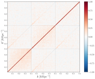
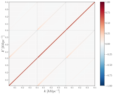
Figure 3 presents the 3 $\times$ 3 blocks of correlation matrices from mock catalogues (left panel) and from the analytic method described in this section (right panel). Correlation coefficients are defined as

$$\mathrm{Corr}(O,O^{{}^{\prime}})=\frac{\operatorname{Cov}(O,O^{{}^{\prime}})}{\sqrt{\operatorname{Cov}(O,O)\operatorname{Cov}(O^{{}^{\prime}},O^{{}^{\prime}})}},$$ (4.6)

where $O\in\{P_{0}(k),P_{2}(k),P_{4}(k)\}$ and $O^{{}^{\prime}}\in\{P_{0}(k^{{}^{\prime}}),P_{2}(k^{{}^{\prime}}),P_{4}(k^{{}^{\prime}})\}$. [23] demonstrates that the analytic Gaussian covariance matrix is in excellent agreement with the mock covariance matrix, and this method is free of the sampling noise with much smaller computational cost, compared to the mocks.

Figure 4: The first six principal components of the $(3\times 3)$ blocks of $P_{l}$ from 1000 MD-PATCHY z3 NGC mock simulations, where $l=0,2,4$. We only include up to four principal components for a low-rank approximation, as the components beyond the fourth are noisy and do not contain much broadband correlations. $\lambda_{i}$ denotes the eigenvalue of the $i$-th eigenvector.

Figure 5: Left: we combine the analytic Gaussian covariance with the smoothed connected pieces obtained from low-rank components with principal component analysis. Right: The difference between the mock and the hybrid covariance which includes the analytic disconnected and smoothed connected covariances, normalized by the diagonal of the latter. Because the connected part is smooth and has a low-rank approximation, we find that only the first four principal components are needed to obtain a smooth estimate of the connected part, and the difference between the mock and its smooth estimate is clean.

4.1.3 Modeling the connected pieces using PCA

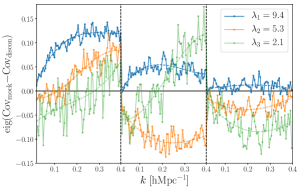
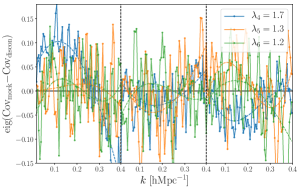
The remaining connected pieces of the covariance matrix, which include Poisson, non-Gaussian (trispectrum) and Gaussian (power spectrum) components, is more difficult to model analytically than the disconnected piece. However, an eigenmode decomposition of the connected components shows that it is a low-rank matrix [45, 46, 47]. In this work, we first obtain the connected parts from the MD-PATCHY mock simulations by subtracting the disconnected parts from the mock covariance matrix and show that this empirical connected piece is indeed a low-rank component with principal component analysis (PCA).

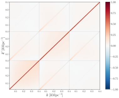
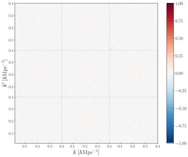
In Figure 4, we perform PCA on the $(3\times 3)$ blocks of $P_{l}$, where $l=0,2,4$, and show its first six principal components. The principal components beyond the fourth component are noisy and do not carry much broadband correlations, and therefore we only include up to four principal components; therefore, the connected components can be well approximated by a low-rank eigen-decomposition. The resulting smoothed connected covariance, combined with the analytic Gaussian covariance, is shown on the left panel of Figure 5, and the right panel shows that it achieves good agreement with the mocks.

4.2 Parameter estimation techniques

In this work, we use the following methods to obtain the parameter posterior distribution: 1) Maximum a posteriori (MAP) estimation and Laplace approximation, using the hessian of the log posterior to obtain the inverse covariance matrix of the model parameters and 2) MCMC sampling of the likelihood, assuming the hybrid covariance matrix with the smoothed connected parts. In section 5.1, we find the best-fitting model parameters for each of the 1000 mock catalogues from MAP estimation and present the 1D histograms and 2D correlations of the cosmological parameters of our interest. Section 6 summarizes the main results of this work: BOSS DR12 RSD measurements of the growth of structure, and we obtain the parameter posteriors using the Python module emcee [48]. [49] presents an optimization-based posterior inference method called EL₂O and shows that the posterior distribution from EL₂O agrees with the MCMC results. Particularly, section 4.4 in [49] discusses how EL₂O can be effective in galaxy clustering analyses. We refer the reader to [49] for more detailed analysis about the comparison between EL₂O and MCMC methods.

5 Model Performance

Figure 6: Left: Maximum a posteriori (MAP) results for 1000 MD-PATCHY z3 NGC (blue) and SGC (red) mock catalogues. We fit the monopole, quadrupole, and hexadecapole over the wavenumber range $0.02<k<0.2\ h$Mpc^-1. 1D distribution of our $f\sigma_{8}$ fit results gives $f\sigma_{8}=0.499\pm 0.038$ and $f\sigma_{8}=0.502\pm 0.058$, for z3 NGC and SGC respectively. The true cosmology indicates $f\sigma_{8}=0.478$, which is 0.4-0.5$\sigma$ away from the mean of our recovered values. Middle, Right: 2D correlations of $f\sigma_{8}$ and $b_{1}\sigma_{8}$ for 1000 MD-PATCHY z3 NGC (blue) and SGC (red) mock catalogues. Vertical dashed line indicates the true cosmology, and solid contours show 1$\sigma$ and 2$\sigma$ confidence regions.

5.1 Tests on the MultiDark-PATCHY mocks

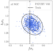
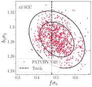
In [1], the accuracy and precision of the power spectrum model in section 3.1 are extensively assessed by performing independent tests using several sets of mocks based on high-fidelity, periodic $N$-body simulations and realistic BOSS DR12 CMASS mocks. The fits typically have a low bias up to $k=0.4$h/Mpc, although for fits with free AP parameter the bias is in some cases significant. We argue in the introduction that this could be caused by a small model misspecification, which can be amplified whenever one must break the degeneracy between two strongly correlated parameters. For this reason we fix AP parameter in this paper. To further confirm that this model is unbiased and accurate enough to provide cosmological parameter constraints of the BOSS DR12 sample, we fit our model to 1000 MD-PATCHY mock catalogues and verify that we can retrieve the true cosmology, provided by the BigMultiDark simulation.

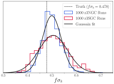
Applying the analysis pipeline in section 4.2 to the mock catalogues, we obtain the best-fitting parameters for each of the 1000 catalogues by first measuring the power spectrum multipoles ($l=0,2,4$) for each of the catalogues and obtaining the MAP estimate using the L-BFGS algorithm. Figure 6 presents the MAP results for 1000 MD-PATCHY z3 NGC (blue) and SGC (red) mock catalogues, and the black dotted vertical line indicates the expected parameter value from the true cosmology of the MD-PATCHY simulations. If we include up to $k_{\mathrm{max}}=0.2\ h$Mpc^-1, we find that $f\sigma_{8}=0.499\pm 0.038$ for z3 NGC and $f\sigma_{8}=0.502\pm 0.058$ for z3 SGC, so we recover the true cosmology ($f\sigma_{8}=0.478$) within 1$\sigma$ with only modest mean biases of $\Delta f\sigma_{8}$ of 0.5$\sigma$.

5.2 Choice of $k_{\mathrm{max}}$

We can further investigate whether the 0.4-0.5 $\sigma$ bias we observe in Figure 6 is caused by the priors or by model misspecification, by comparing it to the analysis where we treat all 1000 mocks as a single dataset. In this case the MAP will be dominated by the likelihood and priors can be ignored. We find $f\sigma_{8}=0.478$ for z1 NGC and $f\sigma_{8}=0.490$ for z3 NGC for $k_{\mathrm{max}}=0.2\ h$Mpc^-1, compared to the truth ($f\sigma_{8}=0.484$ for z1 and 0.478 for z3), both with very small error of order 0.001. In both cases the mean has moved closer to the true value, suggesting the prior is driving the MAP away from the true value, even if there is also some small model misspecification for z3 NGC. If we repeat the analysis for $k_{\mathrm{max}}=0.4\ h$Mpc^-1 we find $f\sigma_{8}=0.498$ for z1 NGC and $f\sigma_{8}=0.497$ for z3 NGC. Now the bias is larger, and suggests more significant model misspecification.

To investigate this further, Figure 7 shows the power spectrum multipole measurements of MD-PATCHY z1 and z3 NGC mock catalogues, along with the best-fit theory lines. Measurements are averaged over 1000 realizations, and the errors are therefore significantly smaller than those of the BOSS survey. Solid and dashed curves indicate convolved and unconvolved best-fit theory curves, respectively. Comparing the upper panel figures (assuming $k_{\mathrm{max}}=0.4\ h$Mpc^-1) with the lower panel figures ($k_{\mathrm{max}}=0.2\ h$Mpc^-1), we find that extending the model to a higher $k_{\mathrm{max}}$ limit makes the model fit noticeably worse at low $k$: both monopole and quadrupole fits with lower $k_{\mathrm{max}}$ have better fits for z1 NGC, and similarly monopole fit has with lower $k_{\mathrm{max}}$ has a better fit for z3 NGC.

Figure 7: Power spectrum multipole measurements (circular points) of MD-PATCHY z1 NGC and z3 NGC mock catalogues and the best-fit theory models. We take 1000 realizations, and the errors are therefore reduced by $\sqrt{1000}$. Solid and dashed curves indicate convolved and unconvolved best-fit theory curves, respectively. The upper panel figures assume $k_{\mathrm{max}}=0.4\ h$Mpc^-1, while the lower panel assumes a lower $k_{\mathrm{max}}$ ($0.2\ h$Mpc^-1 with vertical lines showing the corresponding wavenumber limits to the fits. We find that extending the model to a higher $k_{\mathrm{max}}=0.4\ h$Mpc^-1 limit makes the model fit worse at low $k$, and as a result an incorrect cosmology may be recovered. We do not observe this issue for $k_{\mathrm{max}}=0.2\ h$Mpc^-1.

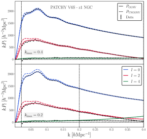
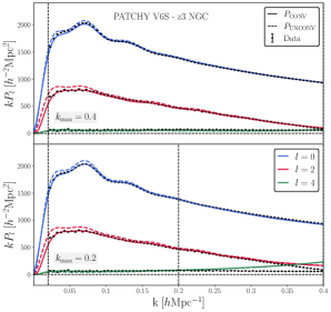
MD-PATCHY mocks are not based on a real N-body simulation, and it is unclear if the galaxy catalogs and the resulting power spectra can be realized in an actual universe. For this reason such comparisons against PATCHY have not been implemented elsewhere, and it is unclear whether we should be concerned given the model is good against real simulations. On the other hand, using 1000 mocks enables one to separate statistical fluctuations from systematics extremely well. In other tests based on one or a few simulation volumes the deviations of recovered cosmological parameters from the truth were within one statistical deviation, in which case it is unclear whether this is a purely statistical effect that can be ignored, or it is a sign of model misspecification, and one must correct for it. As we are unable to answer whether MD-PATCHY power spectra can represent an actual galaxy realization in a real universe, we present both results. However, more caution should be taken when extending to a higher $k_{\mathrm{max}}$, and we argue that a consistent, reliable choice of $k_{\mathrm{max}}$ is one of the major unresolved questions of the RSD analyses. It becomes increasingly difficult to obtain unbiased estimates as we push to higher $k_{\mathrm{max}}$, simply because the fits are dominated by the smallest errors which are close to $k_{\mathrm{max}}$, but cosmology information is entirely extracted by the low $k$ asymptote of the fitted model: even a slight model misspecification at high $k$ can lead to a biased answer at low $k$. Moreover, since we have to fit more parameters to high $k$ the choice of their prior distribution also affects the fits: even a seemingly innocent flat prior choices can project onto a significant bias in the cosmological parameters. Different works choose different values, which may partially explain why results from different studies are discrepant in terms of their $f\sigma_{8}$ measurements.

6 BOSS DR12 RSD measurements

Figure 8: The measured galaxy power spectrum multipoles in Fourier space (circular points with error bars) and the best-fit theory curves (solid lines) for BOSS DR12 z1 (Left panel) and z3 (Right panel) samples. (We only show every other data points for simplicity.) We can fit the model to the monopole (blue), quadrupole (red), and hexadecapole (green), over the wavenumber range $0.02-0.4h$Mpc^-1, with $\Delta k=0.005$, but the choice of $k_{\mathrm{max}}$ may affect the cosmological analysis moderately, as discussed in section 5.2. Following [40], we use a consistent definition of the normalization term for both power spectrum and window function.

Figure 9: Left: 1D and 2D posterior distributions of two selected parameters $f\sigma_{8}$ and $b_{1}\sigma_{8}$ for all galaxy samples with $k_{\mathrm{max}}$=0.2 $h$Mpc^-1. Right: The best-fit $f\sigma_{8}$ values and their 1$\sigma$ uncertainties for the BOSS DR12 sample in two different redshift bins (including both NGC and SGC sky patches). We put the prior on $f$ using the Planck 2018 prior for $\Omega_{m}$ [26]. For all results, we fit to the monopole, quadrupole, and hexadecapole, assuming the full covariance with the smoothed connected parts, as described in section 4.1.3. We also account for the systematic error resulting from the selection of the underlying template cosmology, as described in section 3.1; this increases the overall error by 5%.

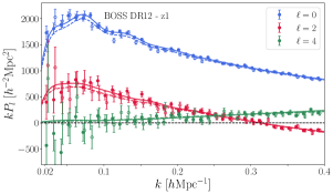
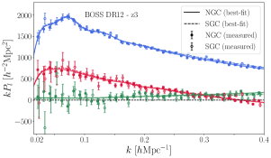
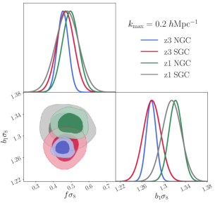
In this section, we present the measurements of the BOSS DR12 galaxy power spectrum multipoles in Fourier space. In figure 8, we show the measured monopole $P_{0}(k)$, quadrupole $P_{2}(k)$, and hexadecapole $P_{4}(k)$ of z1 and z3 galaxies in both NGC and SGC patches, using the FFT-based galaxy power spectrum estimator described in section 3.2. We then fit the RSD model presented in section 3.1 to the measured multipoles and find that the power spectrum multipoles are accurately modeled, in agreement with [1]. In our fits, we set the minimum wavenumber $k_{\mathrm{min}}$ to 0.02$\ h$Mpc^-1 for all samples, in order to minimize any large-scale effects of the window function. As described in section 3.1, we fix the AP distortion parameters to their fiducial values and constrain 11 model parameters ($f(z_{\mathrm{eff}}),\sigma_{8}(z_{\mathrm{eff}}),b_{1,c_{A}},b_{1,s_{A}},b_{1,s_{B}},f_{s},f_{s_{B}},\langle N_{>1,s}\rangle,\sigma_{c},\sigma_{s_{A}},f^{1h}_{s_{B}s_{B}}$), of which two are primarily of our interests: the growth rate $f$ and the amplitude of matter fluctuations $\sigma_{8}$. The Planck satellite provides a strong prior on $f$ with the tight constraint of the matter density $\Omega_{m}$ [26], and we therefore put the Planck 2018 prior on $f$ in all subsequent analyses.

Figure 10: Comparison of $f\sigma_{8}$ constraints to previous BOSS DR12 measurements [5, 3, 6, 7, 10, 9, 11, 13, 12], along with the prediction assuming the Planck 2018 $\Lambda$CDM cosmology (black curve with grey shades) [26]. We show our main results as thick diamonds points, for two $k_{\mathrm{max}}$ limits: 0.2 (sky blue points) and 0.4 $h$Mpc^-1 (dark blue points). We show a partial compilation of other results, which used different methodologies, and cannot always be compared in reported errors. Our results, Alam et al. [3], Ivanov et al. [6], Chen et al. [9], and Kobayashi et al. [11] present measurements of $f\sigma_{8}$ for z1 and z3 galaxy samples ($z_{\mathrm{eff}}=0.38$ and $0.61$, respectively), but for graphical purpose they are plotted at different redshifts. Reid et al. [5], D’amico et al. [7], and Yuan et al. [13] show the constraints on the CMASS sample at $z_{\mathrm{eff}}=0.57,0.55$ and $0.52$, respectively, Lange et al. [10] takes the galaxy samples at $z=0.25$ and $0.4$, and Zhai et al. [12] splits the galaxy sample into three redshift bins at $z_{\mathrm{eff}}=0.25,0.41,$ and $0.56$.

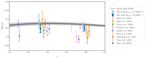
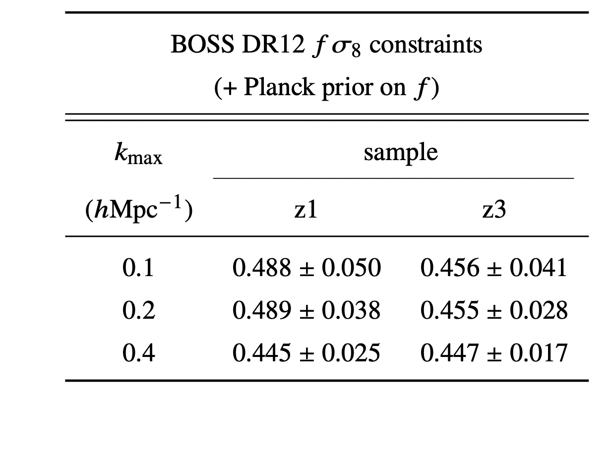
Figure 9, along with the table of $f\sigma_{8}$ constraints with varying $k_{\mathrm{max}}$ cuts, summarizes the main results of our analysis. Fitting our RSD model to the measured BOSS DR12 multipoles (monopole, quadrupole, and hexadecapole) and marginalizing over all nuisance parameters discussed in section 3.1, we obtain the following growth of structure constraints: $f\sigma_{8}(z_{\mathrm{eff}}=0.38)=0.489\pm 0.038$ for z1 sample and $f\sigma_{8}(z_{\mathrm{eff}}=0.61)=0.455\pm 0.028$ for z3 sample, with $k_{\mathrm{max}}=0.2\ h$Mpc^-1. In the table, we also provide the constraints as a function of $k_{\mathrm{max}}$: $f\sigma_{8}(z_{\mathrm{eff}}=0.38)=0.488\pm 0.050$ for z1 and $f\sigma_{8}(z_{\mathrm{eff}}=0.61)=0.456\pm 0.041$ for z3 with $k_{\mathrm{max}}=0.1\ h$Mpc^-1, while $f\sigma_{8}(z_{\mathrm{eff}}=0.38)=0.445\pm 0.025$ for z1 and $f\sigma_{8}(z_{\mathrm{eff}}=0.61)=0.447\pm 0.017$ for z3 with $k_{\mathrm{max}}=0.4\ h$Mpc^-1. For all results, we assume the full covariance with the smoothed connected parts in section 4.1.3, and we also include the systematic error that arises from the selection of the underlying template cosmology, which increases the overall error by 5%. The left panel of Figure 9 also presents the constraints for $b_{1}\sigma_{8}$: with $k_{\mathrm{max}}=0.2\ h$Mpc^-1, we obtain $b_{1}\sigma_{8}(z_{\mathrm{eff}}=0.38)=1.320\pm 0.011$ for z1 and $b_{1}\sigma_{8}(z_{\mathrm{eff}}=0.61)=1.278\pm 0.009$ for z3 sample.

We can translate our constraints in terms of the parameter $S_{8}^{\gamma}\equiv\sigma_{8}(\Omega_{m}/0.3)^{\gamma}$, where $\gamma=\mathrm{dln}f\sigma_{8}/\mathrm{dln}\Omega_{m}\simeq 0.78\cdot(1-\Omega_{m}(z))$ [50]. For the galaxy samples considered in this work and for Planck fiducial value of $\Omega_{m}$ we have $\gamma=0.37$ for z1 and 0.28 for z3, respectively. We find $S_{8}^{\gamma}=0.821\pm 0.040$ and $0.824\pm 0.056$ with $k_{\mathrm{max}}=0.2$ and $0.1\ h$Mpc^-1, respectively, consistent with Planck’s value $S_{8}^{\gamma}\sim 0.83\pm 0.01$ [26]. Extending to a higher $k_{\mathrm{max}}$ of $0.4\ h$Mpc^-1, we get $S_{8}^{\gamma}=0.786\pm 0.025$, about 1.8$\sigma$ lower than the Planck constraint. In section 5.2 we argued that extending the model to $k_{\mathrm{max}}$ of $0.4\ h$Mpc^-1 may lead to model misspecification. We note that for RSD $\gamma$ is lower than in weak lensing (where typically $\gamma>0.5$), so RSD and weak lensing do not measure the same combination of $\sigma_{8}$ and $\Omega_{m}$ as encoded in $S_{8}^{\gamma}$. Specifically, RSD is more sensitive to $\sigma_{8}$ only, specially at higher redshifts.

Figure 10 compares our $f\sigma_{8}$ measurements to previous BOSS DR12 results in the literature [5, 3, 6, 7, 10, 9, 11, 13, 12], along with the constraint assuming the Planck 2018 $\Lambda$CDM cosmology [26]. [3] divides the BOSS galaxies into three redshift bins ($z_{1},z_{2}$ and $z_{3}$) and provides the “consensus” $f\sigma_{8}$ constraints by combining measurements from seven companion papers. Our constraints are not in tension with the consensus analysis (with $k_{\mathrm{max}}=0.2\ h$Mpc^-1, $0.21\sigma$ lower for z1 and $0.68\sigma$ higher for z3) or with the Planck 2018 predictions (with $k_{\mathrm{max}}=0.2\ h$Mpc^-1, $0.37\sigma$ higher for z1 and $0.49\sigma$ lower for z3), while providing one of the tightest constraints on $f\sigma_{8}$ among recent works.

Figure 11 shows how different combination of dataset, wavenumber range, and covariance matrices may affect the cosmological analysis. With $k_{\mathrm{max}}=0.2\ h$Mpc^-1, we obtain $f\sigma_{8}=0.450\pm 0.032$ for z3 NGC, assuming the full covariance including connected parts. Extending $k_{\mathrm{max}}$ to $0.4\ h$Mpc^-1 tightens the constraint significantly, while shifting the best-fitting parameter mean modestly ($f\sigma_{8}=0.458\pm 0.021$). The dotted curves in the left panel present the constraint assuming the analytic disconnected covariance ($f\sigma_{8}=0.453\pm 0.029$ and $0.461\pm 0.018$ for $k_{\mathrm{max}}=0.2$ and $0.4\ h$Mpc^-1, respectively), and we thus find that including the connected parts inflates its standard deviation by 10-20%.

Figure 11: $f\sigma_{8}$ constraints of the BOSS DR12 z3 NGC sample, varying dataset, wavenumber range, and covariance matrices. Left: Constraints obtained with different covariances matrices in section 4.1. Adding the connected parts (blue) to the analytic disconnected covariance (red) weakens our constraints by 10-20%. We also show the impact of including wavenumbers in a wider range. Dashed curves assume $k_{\mathrm{max}}=0.2$ $h$Mpc^-1, and extending it to 0.4 $h$Mpc^-1 (solid curves) improves our constraints considerably. Right: Results obtained with the inclusion (green) or exclusion (orange) of the hexadecapole to quantify its impact on $f\sigma_{8}$ constraints. Excluding the hexadecapole inflates its standard deviation by 15-30%. For both results, we assume the full covariance matrix with the connected part.

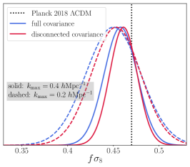
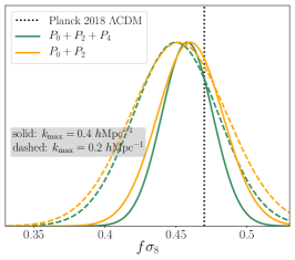
In the right panel of Figure 11, we show results of fitting only the monopole $P_{0}$ and quadrupole $P_{2}$ to quantify the impact of including hexadecapole $P_{4}$ on our constraints on the growth of structure. With $P_{0}$ and $P_{2}$ only, we obtain $f\sigma_{8}=0.452\pm 0.035$ and $0.460\pm 0.025$ for $k_{\mathrm{max}}=0.2$ and $0.4\ h$Mpc^-1, respectively, and find that the best-fit parameter mean remains consistent, while the standard deviation of $f\sigma_{8}$ increases by 15-30%, which is consistent with [51]. Therefore, we include the hexadecapole $P_{4}(k)$ in our main analysis (presented in Figure 9) because this improves RSD constraints significantly, as reported earlier in [52], [53], and [1].

Figure 12: The ratio of the wiggle ($P_{\mathrm{W}}$) to the no-wiggle ($P_{\mathrm{NW}}$) poles of the BOSS DR12 z3 NGC galaxy power spectrum using the best-fit cosmology. The ratio for the monopole, quadrupole, and hexadecapoles are shown in the left, middle, and right panels, respectively.

Figure 13: Left: (Top panel) Power spectrum multipole measurements of the BOSS DR12 z3 NGC sample with BAO wiggles. Solid curves indicate the best-fit theory model, convolved with the window function ($P_{\mathrm{CONV}}$). Dashed and dotted curves indicate best-fit unconvolved ($P_{\mathrm{UNCONV}}$) and linear ($P_{\mathrm{LIN}}$) theory models, respectively. (Bottom panel) We take the BAO wiggle template from figure 12 and subtract it from the measured data so that we can get the “no-wiggle” measurements. All best-fit theory lines also assume the models without BAO wiggles. Right: The model constraint with the full power spectrum and the no-wiggle fit with the fixed fiducial BAO template. Fitting to $k_{\mathrm{max}}=0.2h$Mpc^-1, we obtain $f\sigma_{8}(z_{\mathrm{eff}}=0.61)=0.450\pm 0.032$ and $0.459\pm 0.033$ with and without BAO, respectively. Therefore, we argue that fixing the BAO information with the fiducial BAO template does not affect the cosmology considerably, which eliminates the need to do a joint power spectrum BAO covariance analysis on mocks.

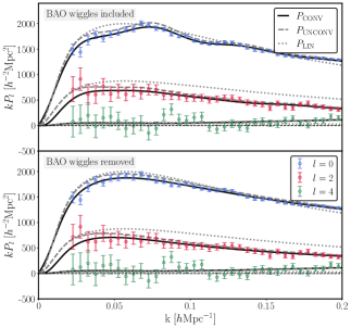
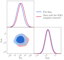
In Figure 12 and Figure 13, we study the sensitivity of cosmological analysis to adding a fixed BAO template to the galaxy power spectrum model. The motivation for this analysis is that there is BAO information in reconstruction, but there is also BAO information in P(k). The two are not independent, and BAO information should not be counted twice. In the past SDSS team used covariance matrix from mocks to identify the amount of correlation. While we do not do BAO analysis here since we fix cosmology parameters other than $f\sigma_{8}$, it is worth asking how to avoid double counting of BAO information in such analysis other than building the full covariance matrix.

Figure 12 shows the ratio of the wiggle ($P_{\mathrm{W}}$) to the no-wiggle ($P_{\mathrm{NW}}$) poles of the BOSS DR12 z3 NGC galaxy power spectrum using the best-fit cosmology; we use the wiggle only nonlinear damping from [54] for BAO models. With this ratio, we create a fixed template for BAO wiggles and subtract it from the multipole measurements to get no-wiggle data. The left panel of Figure 13 shows z3 NGC multipole measurements (circular points with error bars): full data with BAO wiggles included (top) and data with BAO wiggles removed (bottom). Subsequently, we fit the theory model to both datasets, full and no-wiggle, and compare their $f\sigma_{8}$ constraints. The right panel of Figure 13 shows that the model constraints for both samples. Fitting to $k_{\mathrm{max}}=0.2h$Mpc^-1, we obtain $f\sigma_{8}(z_{\mathrm{eff}}=0.61)=0.450\pm 0.032$ and $0.459\pm 0.033$ with and without BAO, respectively; we find that removing BAO information does not shift the model parameter constraints significantly and fixing the BAO information with the fiducial template only minimally affects the cosmology. This result suggests a simplified large-scale structure analyis where the BAO information is completely independent of the de-wiggled power spectrum analysis, without a need to compute their covariance from mocks, as is commonly done when combining BAO reconstruction and RSD analyses.

7 Conclusion

We have presented the analysis of the SDSS-III BOSS DR12 galaxy sample, employing the redshift-space galaxy power spectrum model of [1], which can accurately model the monopole, quadrupole, and hexadecapole down to small scales. With the Planck 2018 prior on the growth rate $f$, we obtain 7.7% and 6.2% constraints on $f\sigma_{8}$ for BOSS DR12 low-redshift z1 ($z_{\mathrm{eff}}=0.38$) and high-redshift z3 ($z_{\mathrm{eff}}=0.61$) samples, respectively, fitting to $k=0.2\ h$Mpc^-1. The combined error is 5%. Extending the wavenumber range to $k_{\mathrm{max}}=0.4\ h$Mpc^-1, we find significant improvement in our constraint: 5.6% and 3.8% constraints on $f\sigma_{8}$ for z1 and z3 samples, respectively, which correspond to an overall 3.2% constraint. However, tests on MD-PATCHY mock catalogues suggest that the model fit to $k_{\mathrm{max}}>0.2\ h$Mpc^-1 may not be reliable, and more caution should be taken when extending to smaller scales. This is further supported by strong running of $f\sigma_{8}$ with $k_{\mathrm{max}}$ for $z1$ from 0.2 to 0.4 $h$Mpc^-1 seen in Table 9, in contrast to little or no running from 0.1 to 0.2 $h$Mpc^-1. We argue that a consistent choice of $k_{\mathrm{max}}$ is the main challenge of RSD analyses. With respect to the Planck 2018 $\Lambda$CDM cosmology predictions or the DR12 final consensus results, we find no tension in our $f\sigma_{8}$ constraints for $k_{\mathrm{max}}=0.2\ h$Mpc^-1, while being 2 sigma lower for $k_{\mathrm{max}}=0.4\ h$Mpc^-1.

Figure 10 presents a review of literature. Most of the measurements are below Planck, and this has been interpreted as evidence of $\sigma_{8}$ tension with Planck from BOSS RSD (e.g, [14, 55, 56, 57]). However, all the analyses are based on the same underlying data (galaxy positions and redshifts), and one cannot simply average these different analyses. The spread of the results is indicative of either model misspecification of some or all of the models, of the influence of the choice of priors, or of the choices made in the analysis, such as the scale cut $k_{\mathrm{max}}$ in power spectrum analysis, power spectrum versus correlation function versus wedges analysis, as well as several additional choices. It is perhaps disturbing that the spread is so large given that the underlying data are the same: at one end of the spectrum our results at $k_{\mathrm{max}}=0.2\ h$Mpc^-1 agree with Planck within 0.3 sigma. At the other end of the spectrum some analyses disagree with Planck at 3-4 sigma. These differences need to be understood so that we can establish the existence or absence of $\sigma_{8}$ tension in cosmology. In this paper we argued that simplifying the analysis such that only one parameter is being fitted to RSD provides a way to do the comparison against Planck that is less influenced by prior volume and model misspecification. Furthermore, we argue that AP parameter is strongly constrained by BAO reconstrution and Planck, and should not be allowed to be varied freely in RSD analysis.

We developed the hybrid covariance matrix which combines the analytic disconnected (or more conventionally, “Gaussian”) part [23], which accounts for the window function effect, and simulation-based connected part, smoothed by including up to four principal components. We demonstrate that the difference between the mock covariance and the hybrid covariance is clean, and the hybrid covariance is free from noise and hence more appropriate to be used in the likelihood analysis. Additionally, we show that using the disconnected covariance matrix underestimates the cosmological parameter constraints by 10-20%.

Furthermore, we provide growth of structure constraints without BAO information by constructing a fixed template for BAO wiggles and subtracting it from the BOSS DR12 multipole measurements. Comparing the constraints with and without BAO wiggles, we conclude that removing BAO information does not noticeably shift the cosmological parameter constraints and hence fixing BAO information with the fiducial template affects the cosmology only minimally. This method enables combining the power spectrum and BAO likelihoods independently, rather than computing their covariance matrix with mock simulations.

Finally, we note that the galaxy power spectrum model and analysis pipeline used in this work can be useful for extracting cosmological information from the next-generation galaxy redshift surveys, such as the Dark Energy Spectroscopic Instrument (DESI) [58] and the Euclid [59] and Roman [60] missions. DESI Emission Line Galaxy sample is expected to provide considerably larger constraining power, as its bias is lower and satellite fraction higher than the BOSS high-redshift z3 sample [58].

References

- [1] N. Hand, U. Seljak, F. Beutler and Z. Vlah, Extending the modeling of the anisotropic galaxy power spectrum to , JCAP 1710 (2017) 009 [1706.02362].
- [2] D.J. Eisenstein and W. Hu, Baryonic Features in the Matter Transfer Function, APJ 496 (1998) 605.
- [3] S. Alam, M. Ata, S. Bailey, F. Beutler, D. Bizyaev, J.A. Blazek et al., The clustering of galaxies in the completed SDSS-III Baryon Oscillation Spectroscopic Survey: cosmological analysis of the DR12 galaxy sample, MNRAS 470 (2017) 2617 [1607.03155].
- [4] N. Kaiser, Clustering in real space and in redshift space, MNRAS 227 (1987) 1.
- [5] B.A. Reid, H.-J. Seo, A. Leauthaud, J.L. Tinker and M. White, A 2.5 per cent measurement of the growth rate from small-scale redshift space clustering of SDSS-III CMASS galaxies, Mon. Not. Roy. Astron. Soc. 444 (2014) 476 [1404.3742].
- [6] M.M. Ivanov, M. Simonović and M. Zaldarriaga, Cosmological Parameters from the BOSS Galaxy Power Spectrum, JCAP 05 (2020) 042 [1909.05277].
- [7] G. D’Amico, J. Gleyzes, N. Kokron, K. Markovic, L. Senatore, P. Zhang et al., The Cosmological Analysis of the SDSS/BOSS data from the Effective Field Theory of Large-Scale Structure, JCAP 05 (2020) 005 [1909.05271].
- [8] P. Zhang, G. D’Amico, L. Senatore, C. Zhao and Y. Cai, BOSS Correlation Function analysis from the Effective Field Theory of Large-Scale Structure, JCAP 02 (2022) 036 [2110.07539].
- [9] S.-F. Chen, Z. Vlah and M. White, A new analysis of galaxy 2-point functions in the BOSS survey, including full-shape information and post-reconstruction BAO, JCAP 02 (2022) 008 [2110.05530].
- [10] J.U. Lange, A.P. Hearin, A. Leauthaud, F.C. van den Bosch, H. Guo and J. DeRose, Five per cent measurements of the growth rate from simulation-based modelling of redshift-space clustering in BOSS LOWZ, Mon. Not. Roy. Astron. Soc. 509 (2021) 1779 [2101.12261].
- [11] Y. Kobayashi, T. Nishimichi, M. Takada and H. Miyatake, Full-shape cosmology analysis of the SDSS-III BOSS galaxy power spectrum using an emulator-based halo model: A 5% determination of 8, Phys. Rev. D 105 (2022) 083517 [2110.06969].
- [12] Z. Zhai, J.L. Tinker, A. Banerjee, J. DeRose, H. Guo, Y.-Y. Mao et al., The Aemulus Project V: Cosmological constraint from small-scale clustering of BOSS galaxies, 2203.08999.
- [13] S. Yuan, L.H. Garrison, D.J. Eisenstein and R.H. Wechsler, Stringent constraints from small-scale galaxy clustering using a hybrid MCMC+emulator framework, 2203.11963.
- [14] M.M. Ivanov, Cosmological constraints from the power spectrum of eBOSS emission line galaxies, Phys. Rev. D 104 (2021) 103514 [2106.12580].
- [15] M.J. Chapman et al., The completed SDSS-IV extended Baryon Oscillation Spectroscopic Survey: measurement of the growth rate of structure from the small-scale clustering of the luminous red galaxy sample, 2106.14961.
- [16] T. Okumura, N. Hand, U. Seljak, Z. Vlah and V. Desjacques, Galaxy power spectrum in redshift space: combining perturbation theory with the halo model, Phys. Rev. D92 (2015) 103516 [1506.05814].
- [17] U. Seljak and P. McDonald, Distribution function approach to redshift space distortions, JCAP 1111 (2011) 039 [1109.1888].
- [18] T. Okumura, U. Seljak and V. Desjacques, Distribution function approach to redshift space distortions. Part III: halos and galaxies, J. Cosmology Astropart. Phys. 2012 (2012) 014 [1206.4070].
- [19] T. Okumura, U. Seljak, P. McDonald and V. Desjacques, Distribution function approach to redshift space distortions. Part II: N-body simulations, J. Cosmology Astropart. Phys. 2012 (2012) 010 [1109.1609].
- [20] Z. Vlah, U. Seljak, P. McDonald, T. Okumura and T. Baldauf, Distribution function approach to redshift space distortions. Part IV: perturbation theory applied to dark matter, J. Cosmology Astropart. Phys. 2012 (2012) 009 [1207.0839].
- [21] Z. Vlah, U. Seljak, T. Okumura and V. Desjacques, Distribution function approach to redshift space distortions. Part V: perturbation theory applied to dark matter halos, JCAP 1310 (2013) 053 [1308.6294].
- [22] J. Blazek, M. McQuinn and U. Seljak, Testing the tidal alignment model of galaxy intrinsic alignment, J. Cosmology Astropart. Phys. 5 (2011) 10 [1101.4017].
- [23] Y. Li, S. Singh, B. Yu, Y. Feng and U. Seljak, Disconnected covariance of 2-point functions in large-scale structure, J. Cosmology Astropart. Phys. 2019 (2019) 016 [1811.05714].
- [24] T. Nishimichi, G. D’Amico, M.M. Ivanov, L. Senatore, M. Simonović, M. Takada et al., Blinded challenge for precision cosmology with large-scale structure: Results from effective field theory for the redshift-space galaxy power spectrum, Phys. Rev. D 102 (2020) 123541 [2003.08277].
- [25] A.G. Sánchez, R. Scoccimarro, M. Crocce, J.N. Grieb, S. Salazar-Albornoz, C. Dalla Vecchia et al., The clustering of galaxies in the completed SDSS-III Baryon Oscillation Spectroscopic Survey: Cosmological implications of the configuration-space clustering wedges, MNRAS 464 (2017) 1640 [1607.03147].
- [26] Planck collaboration, Planck 2018 results. VI. Cosmological parameters, Astron. Astrophys. 641 (2020) A6 [1807.06209].
- [27] M.R. Blanton, H. Lin, R.H. Lupton, F.M. Maley, N. Young, I. Zehavi et al., An Efficient Targeting Strategy for Multiobject Spectrograph Surveys: the Sloan Digital Sky Survey “Tiling” Algorithm, AJ 125 (2003) 2276 [arXiv:astro-ph/0105535].
- [28] A.S. Bolton, D.J. Schlegel, É. Aubourg, S. Bailey, V. Bhardwaj, J.R. Brownstein et al., Spectral Classification and Redshift Measurement for the SDSS-III Baryon Oscillation Spectroscopic Survey, AJ 144 (2012) 144 [1207.7326].
- [29] C.P. Ahn, R. Alexandroff, C. Allende Prieto, S.F. Anderson, T. Anderton, B.H. Andrews et al., The Ninth Data Release of the Sloan Digital Sky Survey: First Spectroscopic Data from the SDSS-III Baryon Oscillation Spectroscopic Survey, ApJS 203 (2012) 21 [1207.7137].
- [30] K.S. Dawson, D.J. Schlegel, C.P. Ahn, S.F. Anderson, É. Aubourg, S. Bailey et al., The Baryon Oscillation Spectroscopic Survey of SDSS-III, AJ 145 (2013) 10 [1208.0022].
- [31] S.A. Smee, J.E. Gunn, A. Uomoto, N. Roe, D. Schlegel, C.M. Rockosi et al., The Multi-object, Fiber-fed Spectrographs for the Sloan Digital Sky Survey and the Baryon Oscillation Spectroscopic Survey, AJ 146 (2013) 32 [1208.2233].
- [32] S. Alam, F.D. Albareti, C. Allende Prieto, F. Anders, S.F. Anderson, T. Anderton et al., The Eleventh and Twelfth Data Releases of the Sloan Digital Sky Survey: Final Data from SDSS-III, ApJS 219 (2015) 12 [1501.00963].
- [33] A.J. Ross, W.J. Percival, A.G. Sánchez, L. Samushia, S. Ho, E. Kazin et al., The clustering of galaxies in the SDSS-III Baryon Oscillation Spectroscopic Survey: analysis of potential systematics, MNRAS 424 (2012) 564 [1203.6499].
- [34] F.-S. Kitaura, S. Rodríguez-Torres, C.-H. Chuang, C. Zhao, F. Prada, H. Gil-Marín et al., The clustering of galaxies in the SDSS-III Baryon Oscillation Spectroscopic Survey: mock galaxy catalogues for the BOSS Final Data Release, MNRAS 456 (2016) 4156 [1509.06400].
- [35] F. Beutler, E. Castorina and P. Zhang, Interpreting measurements of the anisotropic galaxy power spectrum, JCAP 03 (2019) 040 [1810.05051].
- [36] F. Beutler, C. Blake, M. Colless, D.H. Jones, L. Staveley-Smith, G.B. Poole et al., The 6dF Galaxy Survey: z 0 measurements of the growth rate and , Monthly Notices of the Royal Astronomical Society 423 (2012) 3430.
- [37] F. Beutler, H.-J. Seo, A.J. Ross, P. McDonald, S. Saito, A.S. Bolton et al., The clustering of galaxies in the completed SDSS-III Baryon Oscillation Spectroscopic Survey: baryon acoustic oscillations in the Fourier space, MNRAS 464 (2017) 3409 [1607.03149].
- [38] N. Hand, Y. Li, Z. Slepian and U. Seljak, An optimal FFT-based anisotropic power spectrum estimator, JCAP 1707 (2017) 002 [1704.02357].
- [39] K. Yamamoto, M. Nakamichi, A. Kamino, B.A. Bassett and H. Nishioka, A Measurement of the quadrupole power spectrum in the clustering of the 2dF QSO Survey, Publ. Astron. Soc. Jap. 58 (2006) 93 [astro-ph/0505115].
- [40] F. Beutler and P. McDonald, Unified galaxy power spectrum measurements from 6dFGS, BOSS, and eBOSS, JCAP 11 (2021) 031 [2106.06324].
- [41] M.J. Wilson, J.A. Peacock, A.N. Taylor and S. de la Torre, Rapid modelling of the redshift-space power spectrum multipoles for a masked density field, MNRAS 464 (2017) 3121 [1511.07799].
- [42] N. Hand, Y. Feng, F. Beutler, Y. Li, C. Modi, U. Seljak et al., nbodykit: an open-source, massively parallel toolkit for large-scale structure, The Astronomical Journal 156 (2018) 160.
- [43] M. Sinha and L. Garrison, “Corrfunc: Blazing fast correlation functions on the CPU.” Astrophysics Source Code Library, Mar., 2017.
- [44] J. Hartlap, P. Simon and P. Schneider, Why your model parameter confidences might be too optimistic. Unbiased estimation of the inverse covariance matrix, aap 464 (2007) 399 [arXiv:astro-ph/0608064].
- [45] J. Harnois-Déraps and U.-L. Pen, Non-Gaussian error bars in galaxy surveys - I, MNRAS 423 (2012) 2288 [1109.5746].
- [46] I. Mohammed, U. Seljak and Z. Vlah, Perturbative approach to covariance matrix of the matter power spectrum, MNRAS 466 (2017) 780 [1607.00043].
- [47] D. Wadekar, M.M. Ivanov and R. Scoccimarro, Cosmological constraints from BOSS with analytic covariance matrices, Phys. Rev. D 102 (2020) 123521 [2009.00622].
- [48] D. Foreman-Mackey, D.W. Hogg, D. Lang and J. Goodman, emcee: The MCMC Hammer, PASP 125 (2013) 306 [1202.3665].
- [49] U. Seljak and B. Yu, Posterior inference unchained with EL_2O, arXiv e-prints (2019) arXiv:1901.04454 [1901.04454].
- [50] L. Kazantzidis and L. Perivolaropoulos, Evolution of the tension with the Planck15/CDM determination and implications for modified gravity theories, Phys. Rev. D 97 (2018) 103503 [1803.01337].
- [51] F. Beutler, H.-J. Seo, S. Saito, C.-H. Chuang, A.J. Cuesta, D.J. Eisenstein et al., The clustering of galaxies in the completed SDSS-III Baryon Oscillation Spectroscopic Survey: anisotropic galaxy clustering in Fourier space, MNRAS 466 (2017) 2242 [1607.03150].
- [52] BOSS collaboration, The clustering of galaxies in the completed SDSS-III Baryon Oscillation Spectroscopic Survey: Anisotropic galaxy clustering in Fourier-space, Mon. Not. Roy. Astron. Soc. 466 (2017) 2242 [1607.03150].
- [53] J.N. Grieb, A.G. Sánchez, S. Salazar-Albornoz, R. Scoccimarro, M. Crocce, C. Dalla Vecchia et al., The clustering of galaxies in the completed SDSS-III Baryon Oscillation Spectroscopic Survey: Cosmological implications of the Fourier space wedges of the final sample, ArXiv e-prints (2016) [1607.03143].
- [54] Z. Vlah, U. Seljak, M. Yat Chu and Y. Feng, Perturbation theory, effective field theory, and oscillations in the power spectrum, JCAP 2016 (2016) 057 [1509.02120].
- [55] O.H.E. Philcox and M.M. Ivanov, BOSS DR12 full-shape cosmology: CDM constraints from the large-scale galaxy power spectrum and bispectrum monopole, PRD 105 (2022) 043517 [2112.04515].
- [56] P. Zhang, G. D’Amico, L. Senatore, C. Zhao and Y. Cai, Boss correlation function analysis from the effective field theory of large-scale structure, Journal of Cosmology and Astroparticle Physics 2022 (2022) 036.
- [57] S.-F. Chen, M. White, J. DeRose and N. Kokron, Cosmological analysis of three-dimensional boss galaxy clustering and planck cmb lensing cross correlations via lagrangian perturbation theory, arXiv preprint arXiv:2204.10392 (2022) .
- [58] DESI Collaboration, A. Aghamousa, J. Aguilar, S. Ahlen, S. Alam, L.E. Allen et al., The DESI Experiment Part I: Science,Targeting, and Survey Design, ArXiv e-prints (2016) [1611.00036].
- [59] R. Laureijs, J. Amiaux, S. Arduini, J.L. Auguères, J. Brinchmann, R. Cole et al., Euclid Definition Study Report, arXiv e-prints (2011) arXiv:1110.3193 [1110.3193].
- [60] O. Doré, C. Hirata, Y. Wang, D. Weinberg, I. Baronchelli, A. Benson et al., WFIRST Science Investigation Team “Cosmology with the High Latitude Survey” Annual Report 2017, ArXiv e-prints (2018) [1804.03628].