Anomalous relaxation of density waves in a ring-exchange system

Abstract

We present the analysis of the slowing down exhibited by stochastic dynamics of a ring-exchange model on a square lattice, by means of numerical simulations. We find the preservation of coarse-grained memory of initial state of density-wave types for unexpectedly long times. This behavior is inconsistent with the prediction from a low frequency continuum theory developed by assuming a mean field solution. Through a detailed analysis of correlation functions of the dynamically active regions, we exhibit an unconventional transient long ranged structure formation in a direction which is featureless for the initial condition, and argue that its slow melting plays a crucial role in the slowing-down mechanism. We expect our results to be relevant also for the dynamics of quantum ring-exchange dynamics of hard-core bosons and more generally for dipole moment conserving models.

I Introduction

The field of dynamics in isolated quantum systems has recently received an increasing amount of attention thanks to the discoveries of a plethora of interesting non-equilibrium behaviors Calabrese (2018); Garrahan (2018); Gogolin and Eisert (2016), and of versatile experimental platforms to realize the same Browaeys and Lahaye (2020); Gross and Bloch (2017). These studies have been partially motivated by the desire to achieve the protection of quantum information from scrambling caused by Hamiltonian dynamics or environmental noise. This has lead to the rapid development of the field of many body localization Abanin et al. (2019); Alet and Laflorencie (2018); Abanin and Papić (2017); Luitz et al. (2015), which relies on strong disorder to provide a safeguard against scrambling many body dynamics, and the nascent field of Hilbert space fragmentation Sala et al. (2020); Khemani et al. (2020); Moudgalya et al. (2021); Yang et al. (2020); Mukherjee et al. (2021); Karpov et al. (2021), which results from the highly constrained configuration space of Hamiltonians with a large number of strong local constraints and/or highly frustrated interactions Zhang and Røising (2022); Sikora et al. (2011).

A milder version of the total arresting of dynamics generated by the phenomena mentioned above is realized by systems which approach equilibrium in a manner which is qualitatively different from standard diffusion. An example of this has recently been explored for the spin-1/2 Heisenberg chain as well as its classical version at intermediate energies where evidence of super-diffusion has recently been seen both theoretically Ilievski et al. (2018); McRoberts et al. (2022) and experimentally Scheie et al. (2021), leading to connections to surface growth dynamics studied by Kardar-Parisi-Zhang Weiner et al. (2020); Kardar et al. (1986). An approach to equilibrium which is slower than that expected from diffusion has also been realized in systems which conserve higher moments (such as dipolar and octupolar) of the spin configuration Iaconis et al. (2019); Feldmeier et al. (2020); Morningstar et al. (2020); Iaconis et al. (2021); Richter and Pal (2022). For two- and higher-dimensional systems, this has also lead to the realization of exotic fractonic phases Gromov et al. (2020); Nandkishore and Hermele (2019); Pretko et al. (2020). Remarkable advances have also been made on probing experimental realizations of Hilbert space fragmentation and/or higher-moment conservation and associated sub-diffusion Guardado-Sanchez et al. (2020); Scherg et al. (2021); Kohlert et al. (2021).

While progress has been made on the analytical description and experimental detection of the phenomena mentioned above, there has been a dire need for numerical simulations on microscopic models to lend support to many of the predictions. This is in general a difficult task as powerful methods to simulate large-scale quantum dynamics on the needed long-time scales are relatively few and capable of handling only specific regimes Baiardi and Reiher (2019); Schmitt and Heyl (2020). It was found insightful Iaconis et al. (2019); Iadecola and Vijay (2020) to adopt methods from stochastic classical mechanics in the framework of cellular automata Iaconis et al. (2019); Gopalakrishnan and Zakirov (2018); Iaconis (2021), which ignore part of the quantum phase fluctuations and have been able to successfully describe the long-term dynamical behavior of strongly interacting quantum systems. This intuition arises from the expectation that for generic systems with sufficiently large Hilbert spaces and for times long compared to the microscopic energy scales of the Hamiltonian, the dynamics does not show quantum coherence, thus reducing to a classical dynamics problem. As mentioned above, well-known exceptions to this exist, but as simulation of exact quantum dynamics is out of reach using current methods, a study of the classical equivalent becomes of particular interest. This can also serve as a natural starting point to understand the complete quantum dynamics. The language of cellular automata also lends itself naturally to a hydrodynamic treatment, which identifies an equivalence between quantum many-body dynamics at late times and classical transport of globally conserved quantities Nahum et al. (2017); Gopalakrishnan (2018); Iaconis (2021). Slow thermalization is often expected in integrable systems described by generalized hydrodynamics Castro-Alvaredo et al. (2016); Bertini et al. (2016). Quantum equivalents of cellular automata, which may be expected to capture the dynamics more accurately, have also been found to share important characteristics of integrable systems Klobas et al. (2021); Alba et al. (2019).

Following up on the studies of constrained systems, we consider in this work the case of a simple hard-core bosonic model living on a square lattice, undergoing ring-exchange dynamics. This model has already been studied from the perspective of cuprates, as they serve as promising candidates to realize high-Tc superconductivity Paramekanti et al. (2002); Rousseau et al. (2005); Schaffer et al. (2009). Although traditionally most studies have focused on the possible exotic ground state features of this model Tay and Motrunich (2010); Tay et al. (2011), some recent works Iaconis et al. (2019); Khudorozhkov et al. (2021) have considered the constrained dynamics generated by the ring-exchange mechanism, including starting from random configurations Iaconis et al. (2019). However, the relevance of fragmentation to generic low-momentum states which are only described by macroscopic patterns has not been investigated.

In this work we address this question using a classical approach based on stochastic dynamics. We find that structured initial configurations in the form of a boson density wave retain their coarse grained structure for a time which grows as a tunable power of the wavelength, with an eventual melting which is approximately described by a continuum model derived from a simple Taylor expansion. We study the detailed structure of the melting process via spatial correlation functions and find that the dynamics proceed through the development of strongly correlated large active regions which merge and destroy the initial modulated pattern.

The detailed plan of the paper is as follows. In Sec.II, we present the model, discuss the quantities conserved under the dynamics, and elucidate the general profile of stripe-like configurations which are perfectly frozen under the dynamics. The bulk of this section discusses the effects of small perturbations on these exactly frozen patterns, and the preservation of the memory of the initial state to infinite times as illustrated by simulation of exact quantum and stochastic classical dynamics on a small system size. The close agreement between exact quantum dynamics and its stochastic classical equivalent seen in this section motivates our approximation and we focus purely on the classical system for the following sections.

Sec.III recalls the expected continuum field theory based on Taylor expansions by first considering the simpler case of correlated random walkers, along with numerical checks of the equations developed. This is followed by a treatment of the hard-core model using a mean-field assumption.

For Sec.IV, we move to more general configurations which take the form of boson density waves, and show the persistence of the memory of the initial state for unexpectedly long periods of time. We also compare the prediction of the continuum field theory developed in Sec.III with the initial dynamics.

We follow up in Sec.V with a detailed analysis of the evolution of the dynamical active regions, and present a phenomenological picture of the mechanism leading up to the melting of the initial density wave configuration.

We summarize our results in Sec.VI and present possibilities for future follow ups via direct simulation of the quantum many body dynamics.

In a following appendix A, we briefly discuss the long-time momentum space profile of correlation functions, show that it is consistent with a mean-field treatment obtained in a previous work, and that it cannot be a basis of the anomalous scaling observed in the present work (as could have been deduced from a recent analysis Sala et al. (2021) of a related model).

II Ring-exchange boson dynamics, conserved quantities and frozen patterns

We consider a system of hard-core bosons living on a square lattice, which evolve stochastically in time using only ring-exchange dynamics where bosons hop by pairs around a 4-sites plaquette of the lattice if and only if a single diagonal of the plaquette is occupied by two bosons (“flippable” plaquettes). This only allowed dynamics is shown in Fig. 1. This dynamic rule trivially conserves the total particle number as well as the number of particles in each individual column and in each individual row Tay and Motrunich (2010); Tay et al. (2011); Iaconis et al. (2019); Khudorozhkov et al. (2021). For the rest of this work, we restrict ourselves to half-filling, i.e. $L^{2}/2$ sites occupied by bosons, on a periodic $L\times L$ lattice, and to the sector where each column and each row has exactly $L/2$ occupied sites. One expects it to be the sector with the largest number of configurations, as it is maximally symmetric. The total number of configurations in this sector can be computed on large lattices using combinatorial techniques Canfield and McKay (2005).

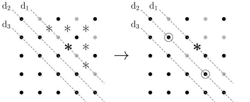
We find that the conserved quantities discussed above do not in themselves completely describe the dynamically connected sets of configurations. This can be seen by considering a “perfect” stripe configuration as shown in Fig. 1, where an alternating pattern of filled and empty sites does not leave a single flippable plaquette, making the configuration frozen under ring-exchange dynamics. By varying the widths and locations of the filled and empty stripes, we can create many similar frozen configurations. One may also naively expect that this restriction on the number of accessible configurations extends to the case where we do not have perfect stripes. To see this, we consider a configuration generated by interchanging the two neighboring diagonals on the edge between a filled and an empty region. This creates a diagonal made of flippable plaquettes, where the influence of this active region may be expected to only extend to a few lattice spacings around this diagonal. Note that similar arguments are expected to hold more general dynamics which conserve the dipole moment. To understand this intuitively, we can consider larger plaquette dynamics, for example 2$\times$1 or 2$\times$2 plaquettes; once again the perfect stripe configuration is frozen and spatial perturbations around it can be expected to at most soften the boundary dynamically, but still leave the stripes intact provided they are wide enough. A simple example of the effect of the 1$\times$1 plaquette dynamics on a boundary between a Néel like (highly active) and a fully filled (inactive) region is shown in Fig. 2. Here one can see that although it is easy to transfer a hole from diagonal $d_{1}$ to $d_{2}$, doing the same for $d_{3}$ would require holes at the circled locations, and thus it is not possible to propagate our excitation into the inactive region without sourcing another flippable plaquette from within the active region.

Figure 1: (a) The ring-exchange rule that is the only allowed dynamics in our system. (b) A perfect stripe configuration which is frozen under the dynamic rule above. (c) Initial configuration with mixed filled-staggered pattern on a $L=16$ sample used to seed Hilbert space fragment. The dynamics of the (d) overlap $O(t)$ and (e) Fourier ratio $R(t)$ with this initial state for both exact dynamics (ED) in the quantum case and stochastic classical automaton (SCA) dynamics, which quickly saturate to the exact values calculated from enumerating all connected configurations.

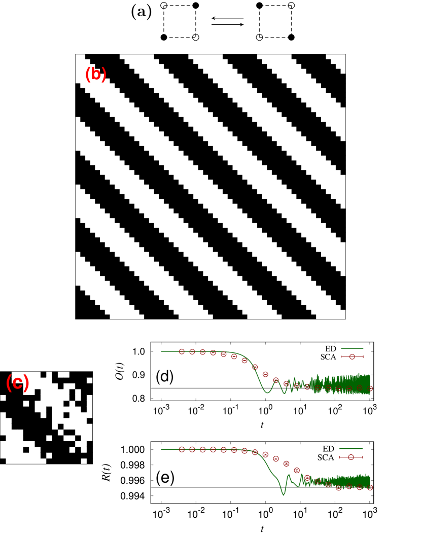
To test this intuition and illustrate this effect, we exactly enumerate all the configurations connected to an initial condition of the form described above (slight random perturbation to the perfect stripe configuration) for a $16\times 16$ lattice (shown in Fig. 1). We find that the total number of configurations, which we call $N_{c}$ which belong to this “fragment” is $27,990$. To show that they retain some structure of the representative which we have chosen, we compute an overlap as defined below,

$$\bar{O}=\frac{4}{N_{c}L^{2}}\sum_{c}\sum_{x,y}n^{\rm seed}_{x,y}n^{c}_{x,y}.$$ (1)

where $n_{x,y}^{c/{\rm seed}}=0,1$ is the number of bosons at site of coordinates $(x,y)$ in the ($c$-th/initial) configuration. If we use all possible configurations (in which case $N_{c}$ would be the total Hilbert space size), we would expect $\bar{O}=0$ due to the symmetry under $n\to 1-n$. For the restricted Hilbert space belonging to the fragment being considered we find $\bar{0}=0.844003...$, showing that for a dynamic simulation restricted to this sector, the initial and late time states would still retain significant overlap. To confirm this, we also run a stochastic classical automaton (SCA) simulation, where at each time step, we propose $L^{2}$ random plaquette flips, and if the chosen plaquette is flippable, we flip it with probability $1/2$. The resulting overlap with the initial state is shown in Fig. 1, and we see that it quickly approaches the value expected from exact enumeration, and retains it indefinitely. To study the accuracy with which the SCA reproduces the exact quantum dynamics, we also perform an exact diagonalization for this Hilbert space fragment, and compute $\braket{\psi(t)}{O}{\psi(t)}$ for $\ket{\psi(t)}=e^{-iHt}\ket{\psi_{0}}$ using $H=\sum_{x,y}b^{\dagger}_{x,y}b_{x+1,y}b_{x,y+1}b^{\dagger}_{x+1,y+1}+h.c.$, where the initial condition is the same occupation-basis state as we initialized the SCA with and $O$ now denotes an operator which is diagonal in the occupation-basis and measures the overlap with the initial state. This operator can be generated directly from the expression above for the classical case by promoting $n^{c}_{x,y}$ to the number operator, while retaining the integer status of $n^{\rm seed}_{x,y}$. As shown in Fig. 1, we find that the overlap in the quantum dynamics closely traces the SCA during the initial decay away from an overlap of $1$.

Figure 2: Illustration of the melting of a Néel-filled boundary: Asterisks mark flippable plaquettes, and the transformation from left to right takes place by an exchange around the plaquette marked by the asterisk in bold type. d_i mark diagonals around the domain boundary.

In the following sections, we quantify the relaxation to equilibrium using the Fourier transform $n_{k}(t)$ with frequency $k$ along the $\hat{x}+\hat{y}$ direction, at time $t$. To this end, we measure the Fourier ratio $R(t)=n_{k}(t)/n_{k}(0)$, and make a similar comparison as done for the spatial overlap above. This is presented in Fig. 1 as well, and once again we find a close agreement between the exact quantum dynamics and it’s classical equivalent in the way they approach the equilibrium value of $R(t)$ within the sector of interest. This result suggests that the quantum dynamics within sectors matches the classical automaton upon coarse graining past time scales of $O$(1), suggesting that quantum phases do not play a substantial role in the aspects of dynamics which we want to study, and that a classical automaton approach could be sufficient to study the effect of the kinetic constraints on large scale features.

Following the arguments above and noting that exact quantum dynamics for larger sizes is not possible with current computational capabilities, we directly study the long time behavior of our stochastic dynamics simulations to gather information about large system sizes in the following sections.

III Expected hydrodynamic description

Here we discuss the coarse grained description in continuous space, of the microscopic dynamics which we have introduced in the previous section. We begin by relaxing the hard-core constraint and considering the limit of average number of particles per site being $\gg 1$. This allows us to reduce the problem to non-interacting correlated random walkers, and leads to an analogue of the diffusion equation which encodes vanilla sub-diffusion. We show numerical evidence for the validity of the same. The expected continuum dynamical behavior of this type of ring-exchange in 2d was first presented in Ref. Iaconis et al. (2019), but we recall it for completeness as well as to understand how it should be perturbed to take into account the hard-core nature. Next we move to an equivalent model of a real-valued field on the lattice which makes the connection to the hydrodynamic limit more transparent, and we again provide support with numerical simulations.

Lastly, we return to the hard-core model presented in the previous section, and show that the continuum theory describing the model must include non-linear terms in addition to the sub-diffusive term, and we show the possibility for a quantitative change in the behavior of the system due to the non-linearities.

III.1 Large particle number limit

We relax the hard-core constraint of the stripe configurations described in the previous section and assume the pattern to exist over a featureless background of an average density of $n_{d}\gg 1$ particles per site. The dynamics can now be understood in terms of correlated random walkers in the following way. First, we label each particle in the system as an independent walker. A move is defined now as first picking a walker (called walker $a$) at random, picking one of its four next nearest neighboring sites with probability $1/4$, and moving one of the walkers on the chosen site (called walker $b$) in tandem with walker $a$ in a ring exchange type manner. Due to the large number of walkers per site, we expect to always be able to find walker $b$.

To write down the number of particles $n$ at a particular position $(x,y)$ at time $t+1$ as a function of the values at time $t$, we must consider all processes which can change $n_{x,y}$. These processes are (1) choosing a walker at $(x,y)$ and moving it away ($\propto n_{x,y}$); (2) choosing a walker at one of the four nearest neighbor sites and moving it or its partner to $(x,y)$ ($\propto 1/2(n_{x\pm 1,y})$ or $1/2(n_{x,y\pm 1})$); (3) choosing one of the walkers at one of the next nearest neighbors and moving it in tandem with a walker at $(x,y)$, thus reducing the number of walkers at $(x,y)$ by one ($\propto 1/4(n_{x\pm 1,y\pm 1})$). Putting these terms together, we can write the change in $n_{x,y}$, which is an whole number, from time $t$ to time $t+1$ as (note that all terms in the expression below are at time $t$, and we do not explicitly mention it for ease of representation)

$$\Delta_{t} n_{x,y}\propto-n_{x,y}$$

$$+\frac{1}{2}[n_{x+1,y}+n_{x-1,y}+n_{x,y+1}+n_{x,y-1}]$$

$$-\frac{1}{4}[n_{x+1,y+1}+n_{x+1,y-1}+n_{x-1,y+1}+n_{x-1,y-1}].$$ (2)

This equation was obtained using similar arguments in Ref. Iaconis et al. (2019). If the system is initialized over a background of $n_{d}$ particles per site using the stripe configuration described in the previous section (shown in Fig. 1), $n_{(x,y)}$ can be seen as a step function switching periodically between $n_{d}$ and $n_{d}+1$. We would naively expect that the correlated dynamics discussed above would quickly eliminate the sharp boundaries of the $n_{(x,y)}$ texture and lead to a smooth function once we average over many realizations of the stochastic dynamics.

For a function which varies slowly as a function of $(x,y)$ (note that this implies that the stripes in the initial condition should be wide compared to lattice spacing), we can perform a Taylor expansion of the expression above. We find that all terms to fourth order cancel, and the only term at fourth order yields

$${\partial_{t}}n_{(x,y)}=-c{\partial_{x}^{2}}{\partial_{y}^{2}}n_{(x,y)}$$ (3)

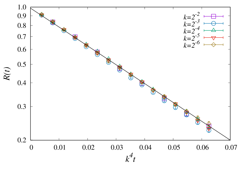
where $c=1$ if following the treatment above. For further convenient reporting of the wave-vector $k$ in units of $\pi$, and taking into account in addition a factor of $4$ coming from the acceptance probabilities in our numerical implementation, we consider instead a different normalization with $c=\pi^{4}/4$. Rescaling the x-axis as in Fig. 3, this allows to recover a match to $e^{-x}$ for the fit in Fig. 3. For the rest of this manuscript, we maintain this convention for $c$.

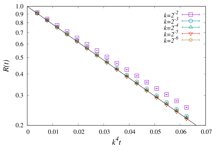
As the stripe initial condition is a periodic square wave in $(x+y)$, it is convenient to rewrite the above equation in the Fourier basis, and consider only the lowest harmonic (largest wavelength) of the square wave transform. This reduces the dynamical equation to ${\partial_{t}}n_{k_{x},k_{y}}=-ck_{x}^{2}k_{y}^{2}n_{k_{x},k_{y}}$. For diagonal stripes, $k_{x}=k_{y}=k$, and $n_{k}$ can be exactly reduced to $n_{k}(0)\exp{(-ck^{4}t)}$, where $n_{k}(0)$ is the value at $t=0$. We can now numerically verify this behavior by calculating the Fourier ratio $R_{k}(t)=n_{k}(t)/n_{k}(0)$, and looking for a data collapse onto a single exponential for various values of $k$. We find that $n_{d}=3$ provides a sufficiently large background for a good data collapse, and show the same for a $128\times 128$ lattice for various stripe widths (encoded in $k$) in Fig. 3 and averaged over $80$ realizations of the stochastic dynamics for each $k$. For smaller values of $n_{d}$, we find an increasing discrepancy between different values of $k$, with the divergence growing with decreasing $n_{d}$.

Figure 3: Dynamics of the ratio $R_{k}(t)=n_{k}(t)/n_{k}(0)$, against $k^{4}t$ for various values of $k$ and on a log-linear scale, for a $128\times 128$ system of correlated walkers, with a background base walker density per site $n_{d}=3$. The solid line is a fit to a single exponential.

III.2 Discretization of continuum equation

Here we study a discretization of Eq. (3) on the lattice by defining the real valued field $n_{x,y}$, and attempt to recover the limit of the hard-core model. From the analysis of the correlated random walkers above, we expect that a ring exchange dynamic on a plaquette should lead to the ${\partial_{x}^{2}}{\partial_{y}^{2}}$ form. To this end, we define the “activity” of a plaquette whose left bottom site is $(x,y)$ to be $a=[n_{x,y+1}-n_{x,y}]-[n_{x+1,y+1}+n_{x+1,y}]$. This is evaluated at time $t$, and the fields living on the plaquette are updated at time $t+1$ by adding $\epsilon a$ to sites $(x,y)$ and $(x+1,y+1)$ and subtracting $\epsilon a$ from the other two sites. The constant $\epsilon$ is included to ensure that the field remains $\in[-1,1]$, and plays only a quantitative role in the scaling study. To deduce the dynamic rule for the activity at a single lattice site, we must consider the four neighboring plaquettes around it which can affect the field on the chosen site via plaquette updates. By summing $a$ for the four plaquettes with equal weight, and carrying out a careful grouping of terms, we see that the equation reduces exactly to the dynamical equation discussed in the previous subsection. Using a Taylor series expansion once again leads to a dynamical equation of the form given in Eq. (3). We attempt a data collapse for the decay of $R(t)$ as defined in the previous subsection for stripe configurations using the dynamic rule mentioned above. As shown in Fig. 4, we once again find a satisfactory data collapse to a single exponential for a large range of $k$ values.

Before we turn to the case of the hard-core model, we must note that the dynamics described in this subsection differ in one crucial way from the hard-core model. We can see this by considering all the plaquette configurations which yield a non-zero value of $a$ (these are listed in Fig. 5), and observing that only the two completely “flippable” (or equivalently with the largest magnitude of $a$) contribute to dynamics in the hard-core case. This is not the case if one considers the dynamical rule used here and in the previous subsection (all plaquettes with all values of $a$ are updated). We argue in the next subsection that this leads to a strong violation of Eq. (3).

Figure 4: Dynamics of $R(t)$ for a $128\times 128$ system with continuum fields at each lattice site, against $k^{4}t$ for various values of $k$ and on a log-linear scale. The solid line is a fit to a single exponential.

III.3 Continuum theory under the hard-core constraint

Now we turn to the model described in the previous section, and restrict particle number to at most one per site, and dynamics only to proceed via exactly flippable plaquettes. Note that now we cannot define an updated state using just the definition of $a$ as in the previous subsection. We require a function which evaluates to unity only for the two flippable plaquette configurations and zero for all others. For the purpose of this subsection, it is more convenient to set $n_{(x,y)}=1$ for an occupied site and $-1$ for an unoccupied site. It is not apparent if there is a unique function which achieves this, and one of the simplest functions which we were able to find on the plaquette to satisfy these constraints is

$$h=\frac{1}{4}\big{[} (n_{x,y+1}-n_{x,y})-(n_{x+1,y+1}-n_{x+1,y})$$

$$-\frac{1}{4}(\Sigma_{p}n)(n_{x,y}n_{x+1,y}-n_{x+1,y+1}n_{x,y+1})$$

$$\ \ \ \ \ \ \ \times(n_{x,y}n_{x,y+1}-n_{x+1,y}n_{x+1,y+1})\big{]},$$ (4)

where $\Sigma_{p}n=n_{x,y}+n_{x,y+1}+n_{x+1,y+1}+n_{x+1,y}$ is the sum of all $n$ belonging to the plaquette. A careful consideration of the expression above reveals that it generates a value of $\pm 1$ for the flippable plaquettes shown in Fig. 5a, while returning zero for all other configurations (including those in Fig. 5b), thus satisfying our requirements for a hard-core ring exchange. The second term in the above expression is formed by noticing that the only configurations which violated the assignment of values we desired had a difference in the types of pair arrangements on opposite edges. Before performing approximations on this expression to derive a continuum theory, we find that it is convenient to expand the product of the last two bracketed terms discussed above as $(2n_{x+1,y}n_{x,y+1}-2n_{x,y}n_{x+1,y+1})$, where we have used $n_{x,y}^{2}=1$ for all $(x,y)$.

Figure 5: Plaquettes which have a non-zero contribution to dynamics in Sec. III.2. Plaquettes (a) are flippable, and (b) do not contribute under hard-core discrete dynamics of Sec. III.3. For (b), we did not include particle-hole symmetric partners (with black and white dots interchanged) for simplicity.

For the evolution $\Delta_{t}n_{x,y}$ of density of a single site, we must once again consider the four plaquettes in which it participates. The resulting expression has a term identical to the dynamic equation in the previous subsections, but has an important addition in the form of the sum of $\frac{1}{2}(\Sigma_{p}n)(n_{{x^{\prime}},y}n_{x,{y^{\prime}}}-n_{x,y}n_{{x^{\prime}},{y^{\prime}}})$ over the four plaquettes.

To get the continuum limit as done previously, we assume initial conditions with several flippable plaquettes and a smooth density profile which varies slowly spatially. An average over stochastic dynamics and initial conditions thus allows us to replace the terms linear in $n$ with the differential form $-{\partial_{x}^{2}}{\partial_{y}^{2}}g$, where $g$ is a real valued field living in continuous space-time aiming at replacing $n$ (we explicitly distinguish it from $n$ for this subsection due to the correlations possibly generated by the products of $n$).

To understand the behavior of the averaged value of terms such as $n_{x+1,y}n_{x,y+1}$, an important assumption about the correlations has to be made. In the following of this subsection, we work in a mean-field picture ignoring correlation effects and assume that such terms can be rewritten as the product of $g$ at the two points. In doing so, we will be able to derive the complete dynamics only in terms of the field $g$. This mean-field like assumption is true for the initial condition we work with, as it is drawn from an uncorrelated ensemble, but it is not a priori evident if the dynamics maintains this uncorrelated nature or rapidly builds up correlations. The non-linear term $f$ is expressed as

$$(\sum_{x,y}n)(n_{x+1,y}n_{x,y+1}-n_{x,y}n_{x+1,y+1})$$

$$+ (\sum_{x-1,y-1}n)(n_{x,y-1}n_{x-1,y}-n_{x-1,y-1}n_{x,y})$$

$$- (\sum_{x-1,y}n)(n_{x,y}n_{x-1,y+1}-n_{x-1,y}n_{x,y+1})$$

$$- (\sum_{x,y-1}n)(n_{x+1,y-1}n_{x,y}-n_{x,y-1}n_{x+1,y}),$$

where the subscript below the sum indicates the plaquette over which the sum is performed indexed by its left bottom site. Once again we expand the products and ensure that we replace all occurrences of $n_{x,y}^{2}$ with unity for all $(x,y)$. The equation above is thus reduced to a linear combination of single body and three body terms. This can be further reduced by performing the mean field decoupling $\braket{n_{x,y}n_{{x^{\prime}},{y^{\prime}}}n_{{x^{\prime\prime}},{y^{\prime\prime}}}}=\braket{n_{x,y}}\braket{n_{{x^{\prime}},{y^{\prime}}}}\braket{n_{{x^{\prime\prime}},{y^{\prime\prime}}}}=g_{x,y}g_{{x^{\prime}},{y^{\prime}}}g_{{x^{\prime\prime}},{y^{\prime\prime}}}$, followed by a Taylor expansion around the relevant site in the derivatives of $g$. As we began our analysis by considering a sum over the four plaquettes surrounding the site $(x,y)$, symmetry restrictions apply to the terms generated by the Taylor series, which require that only terms with non-zero coefficients have an even number of derivatives in $x$ and $y$, and are symmetric with respect to the $x\to y$ transformation. Using this constraint and after some algebra, we find that the only surviving terms arise at fourth order in the derivatives and that the complete dynamical equation reduces to the following expression (ignoring a global factor of $1/4$), given by

$$\partial_{t}g=-\Big{(}\frac{1}{2}-g^{2}\Big{)} {\partial_{x}^{2}}{\partial_{y}^{2}}g-{\partial_{y}^{2}}g({\partial_{x}}g)^{2}-{\partial_{x}^{2}}g({\partial_{y}}g)^{2}$$

$$-2({\partial_{x}}g)({\partial_{y}}g)({\partial_{x}}{\partial_{y}}g)-g{\partial_{x}^{2}}g{\partial_{y}^{2}}g.$$ (5)

The presence of non-linearities, derived even under a crude mean-field approximation, suggests that at leading order in the dynamics, the hard core constraint indeed plays an important role, and may invalidate the expectation that the coarse grained dynamics are equivalent to those of vanilla sub-diffusion.

IV Long time persistence and eventual melt of approximate stripe configurations

We have seen in the Sec. II that configurations which can be viewed as small perturbations around a perfect stripe configuration may maintain the memory of the initial state indefinitely. As these configurations are highly specific, it would seem unrealistic to choose one of these as the initial state for the dynamics of large systems. This motivated us to study “approximate” stripe patterns, which are chosen to be boson density waves with a wave-vector $\vec{k}=(k_{x},k_{y})$.

Figure 6: (a) A sample boson configuration created by annealing to the target function $f_{\vec{k}}$ Eq. 6 with $k_{x}^{t}=k_{y}^{t}=0.1875$ and $A=1.0$ for a $96\times 96$ lattice, along with (b) Fourier components of random initial states for larger sizes generated using the annealing method for $k_{x}^{t}=k_{y}^{t}=0.1875$, plotted against the nearest distance $k_{d}$, shows a clear peak for $k_{d}=0$.

IV.1 Initial state preparation

To prepare such configurations, we first generate a target distribution using the function

$$f_{\vec{k^{t}}}(\vec{r})=A\sin(\vec{k^{t}}\cdot\vec{r}),$$ (6)

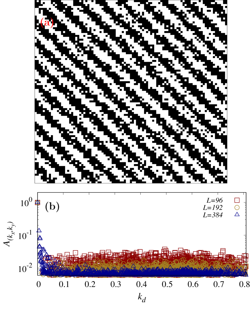
where $A$ takes continuous values between $0$ and $1$. We cannot generate a configuration which has exactly this pattern as a boson configuration can take only $\pm 1$ (filled/empty) at each site. Thus we perform a Monte Carlo simulated annealing starting from a charge-density wave state with $\vec{k^{t}}=k^{t}\hat{e}_{x}+k^{t}\hat{e}_{y}$ using an energy defined as $E=\sum_{l}(D_{l}-Lf_{\vec{k^{t}}}(\vec{r}))^{2}$, where the sum is over all diagonals and $D_{l}=\sum_{(i,j)\in l}\sigma_{i,j}$, is the occupancy in diagonal number $l$. This favors an exact match between the current and target configurations. By tuning the inverse temperature for the annealing from $\beta=0.01$ to $\beta=20.48$ in a geometric progression consisting of multiplying by $2$ every $10L^{2}$ steps, we achieve a stripe configuration which has a single Fourier component at the target $\vec{k^{t}}$. We ensure that the proposed configuration changes are long-ranged and respect the conservation laws discussed in the previous section, thus staying in the sector where every column and every row has exactly $L/2$ bosons. An example of a configuration created by this procedure is shown in Fig. 6a. To check the effectiveness of the annealing procedure, we record the final energy and find it to be $O(L)$, implying that each $D_{l}$ is within an $O(1)$ value of its target value, which is expected as $D_{l}$ is an integer and the target value is in general a real number, and not necessarily close to an integer value. We find that this procedure generates a sharp peak for the desired $\vec{k^{t}}$ amid a weak background which decays with increasing system size. This can be seen in Fig. 6b, where we plot the Fourier component as a function of the distance from the target peak location in Fourier space $k_{d}^{2}=(k_{x}-k^{t})^{2}+(k_{y}-k^{t})^{2}$ for various sizes. Due to the periodic boundary conditions in Fourier space, given by $(k_{x},k_{y})\leftrightarrow(1-k_{x},1-k_{y})$, we consider the shortest distance to the expected peak over the naive distance for open boundary conditions. Note that such a configuration still contains a large number of flippable plaquettes due to the smooth nature of the target pattern.

Figure 7: Plots for $A=0.7$ : (a) Comparison of average scaled profile $B_{x}(t)$ from microscopic hard-core dynamics compared to continuum expression (Eq. (III.3)) for wavelength $\lambda=16$ for $t_{0}=16$. (b) $R(t)=n_{k}(t)/n_{k}(0)$ against $k^{4}t$ on log-linear scale, with long times fit to a single exponential.

IV.2 Comparing with continuum field theory

In the context of the continuum field theory discussed in Sec.IIIC, the field $g$ at time zero would now simply be equal to $A\sin(\vec{k}\cdot\vec{r})$ with $\vec{k}=\vec{k^{t}}$. It is essential to numerically verify the validity of the assumption used in developing our continuum theory, namely that spatial correlations do not play a role in the initial dynamics.

Using this as the initial source field in Eq. (III.3), we find that ${\partial_{t}}g$ reduces to

$$Ak^{4}\sin(\vec{k}\cdot\vec{r})\Big{[}-\frac{1}{2}+4A^{2}\cos^{2}(\vec{k}\cdot\vec{r})-\frac{A^{2}}{2}\sin^{2}(\vec{k}\cdot\vec{r})\Big{]}.$$ (7)

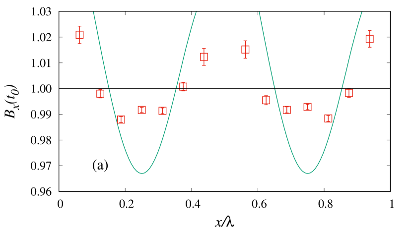
This immediately indicates that we have lost linearity (which would imply no dependence on amplitude other than a global proportionality), and that the theory is no longer exactly separable in Fourier space. Note here that the terms proportional to $A^{2}$ within the brackets oppose the decay generated by the simple sub-diffusion, leading to a possibility of further slowing down the dynamics. The above equation also suggests that for $A\ll 1$, we should expect to recover vanilla sub-diffusive dynamics. For $\vec{k}\cdot\vec{r}\in(0,\pi)$, the sign is controlled by the expression within the brackets, and we can see that a growth of the function can be achieved for $\sin(\vec{k}\cdot\vec{r})<((8A^{2}-1)/(9A^{2}))^{1/2}$, provided $8A^{2}>1$ (that is large enough amplitude). This condition is satisfied for $\vec{k}\cdot\vec{r}$ in the vicinity of $0$ and $\pi$. This effect is rather non-intuitive as it implies that the local density tends away (towards $\pm 1$) from its equilibrium value (0) under non-equilibrium dynamics for a tunable range of $\vec{r}$, leading to a local reduction of entropy as the number of states available locally reduces if we require their average to be closer to the most extreme values which it can take. To ascertain the extent to which our microscopic dynamics is consistent with the continuum field theory developed under the mean field assumption, we can now compare the averaged value of $n_{x,y}$ against a numerical evolution of Eq. (III.3). Looking specifically for the feature described above, we plot $B_{x}(t)=\langle n_{x,x}(t)\rangle/\langle n_{x,x}(0)\rangle$ in Fig. 7a as a function of $x$ for the minimal period. Our initial condition already sets $n_{x,x}(0)=A\sin(2kx)$. We see a qualitative match to the prediction from the continuum equation (in the sense of the sign of the difference to unity of the ratio is well captured), but a quantitative disagreement (in the amplitude of this difference) potentially due to the build up of correlation effects beyond mean-field.

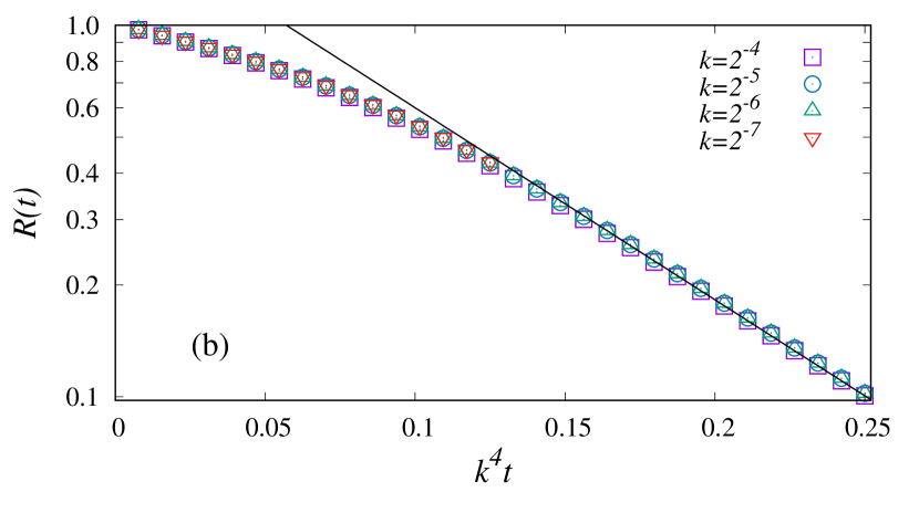
Before we move to the study of the microscopic dynamics, it is worth considering the time scales over which the initial pattern melts under the continuum dynamics, as done in Sec. II. We show in Fig. 7b that the dynamics is still consistent with a single scaling variable, given by $k^{4}t$, although the relaxation deviates from the single exponential seen in the simpler cases considered in Sec. II. This implies that the additional non-linear terms in the continuum dynamics do not alter the scaling of space-time, and this can be intuitively understood by observing that all non-linear terms have the same order in derivatives.

Figure 8: For “weak” amplitude $A=0.2$. (a) Dynamics of $R(t)$ as a function of $k^{4}t$, in a log-linear scale. (b) Zoom on initial dynamics, that shows a consistent scaling with $k^{4}t$ for sample initial conditions. We do not present an average over samples as it leads to large fluctuations over the time axis.

Figure 9: For “large” values of amplitude $A$ : (a) Slow initial behavior of $R(t)$ as a function of time, for $A=0.5$, $k=0.125$ and a $L=256$ sample. To detect the beginning of the melting process, we define a threshold of 0.99 (shown by dotted line), and define $t_{0}$ as the intercept. (b) Average melting starting time $t_{0}$ as a function of $1/k$, for different values of $A$. The log-log scale emphasizes the power-law dependence. The black solid line corresponds to a $1/k^{4}$ power-law.

IV.3 Exact numerical evolution: Beginning of melting

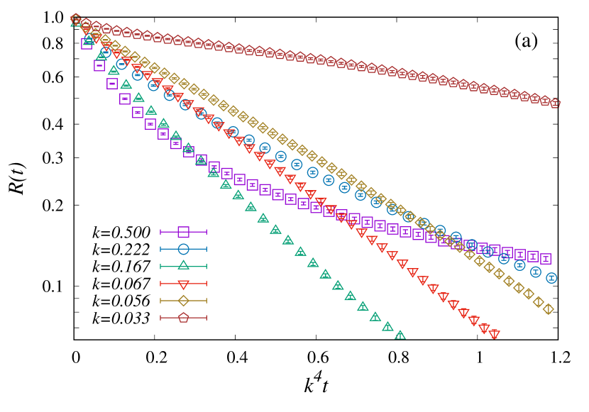
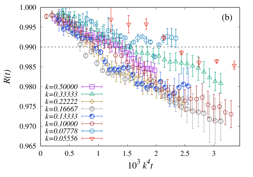
We now study the dynamical behavior starting from a configuration generated by the method discussed above. To carry out an analysis of the evolution of the coarse-grained structure of the initial configuration, we choose to study the decay of the dominant Fourier component via the already defined ratio $R(t)=\frac{n_{\vec{k}}(t)}{n_{\vec{k}}(0)}$. To get an intuition about the effect of lattice spacing, we first consider the decay of $R(t)$ over a range of decreasing values of $k$, starting from $k=1/2$. As shown in Fig. 8a, for $A=0.2$, there are clear deviations away from a single exponential for large values of $k$, whereas intermediate values of $k$ appear to agree partially, and for small values of $k$, we once again deviate from the expected $k^{-4}$ scaling. To study the initial stages of the decay of the wave pattern, we can look at $R(t)$ in the regime where it is close to unity. Here we find a collapse consistent with a time scaling with $k^{-4}$ for a large range of $k$, including large $k$ values (as shown in Fig. 8b). This is quite surprising, because the regime of short-time scales and large-wave vectors is not the one where we expect the hydrodynamic prediction of Sec. III to hold. We have no simple explanation for this observation.

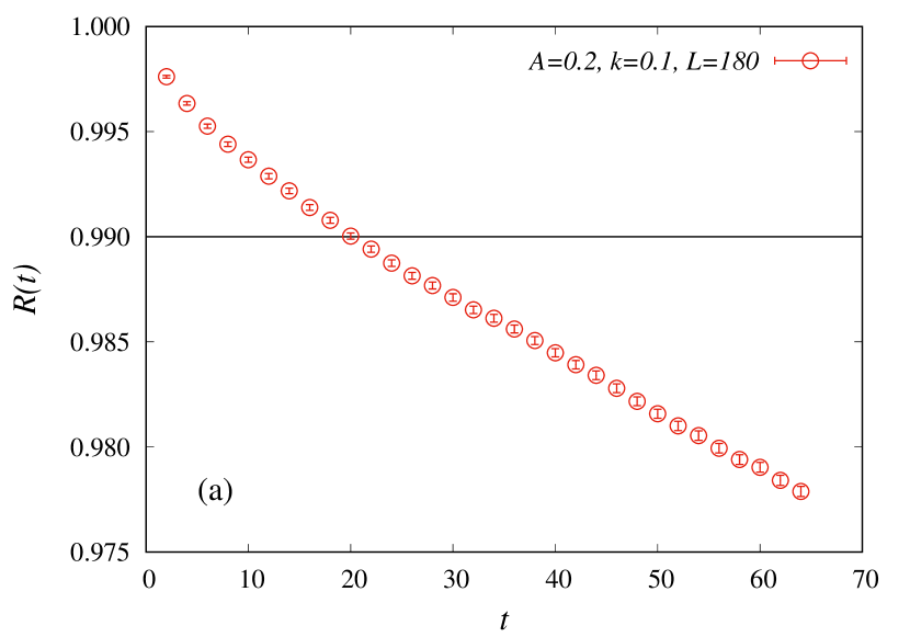
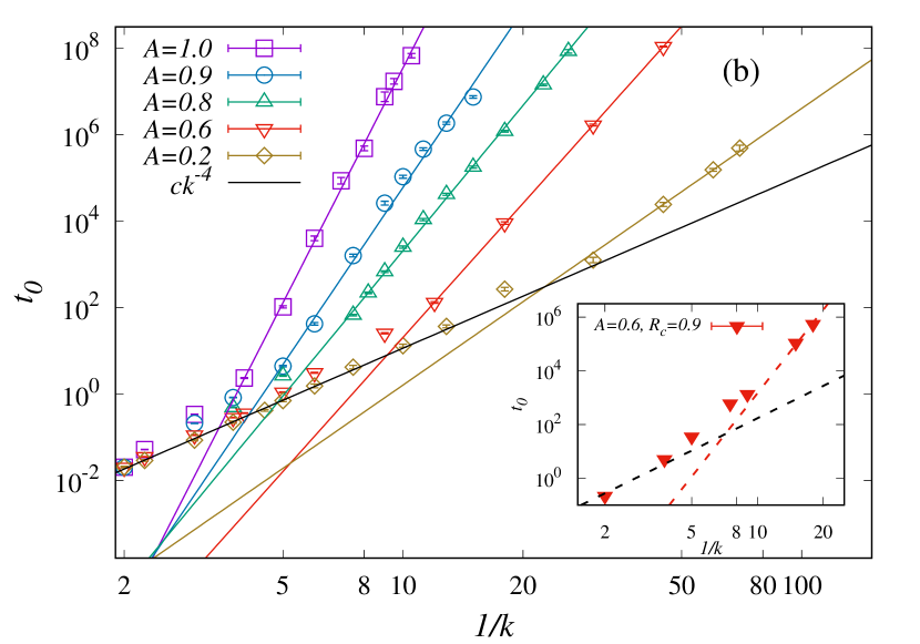
For larger values of $A$, we observe a completely different behavior. We find that $R(t)\approx 1$ for a non-trivial amount of time after the initialization of the dynamics, an illustration of this behavior of $R(t)$ is given in Fig. 9 for $A=0.5$. We define the beginning of the melting process by the first time $t_{0}$ at which $R(t)$ crosses $0.99$. This threshold is chosen arbitrarily and a different threshold does not change the result qualitatively (as shown using a threshold of $0.9$ in the inset of Fig. 9b). We study this for a few values of $k$, and for $20$ realizations of the initial condition for each $k$. In addition to this, for each realization, we run sufficient number of realization of the stochastic dynamics to ensure that we get a good estimate for $t_{0}$. We have taken systems of linear size in the range of $150-250$, as the property of self-averaging allows us to narrow the spread in the values of $t_{0}$. We find a strong dependence of the averaged $t_{0}$ on the inverse wave-vector $1/k$. A linear fit on a log-log scale of $t_{0}$ vs $1/k$ reveals various power law regimes (see Fig. 9b) that depend on the amplitude $A$, the most extreme of which is achieved for $A=1$, where the dependence is $t_{0}\sim(1/k)^{18.1(3)}$. Such a strong dependence on the initial pattern suggests that the mechanism for melting is initiated by a coordinated rearrangement of bosons which is favorable for dynamics. Note that for all values of $A$, there exists a window of $1/2>k>k^{0}(A)$, where we find good agreement with $(1/k)^{4}$, as predicted from the continuum theory, with $k^{0}(A)$ reducing with reducing $A$.

IV.4 Exact numerical evolution: Post-melt scaling

The continuum theory developed in Sec. III, which can be valid only for small wave-vectors and long times, cannot describe the results in Fig. 9b and the period for which we observed $R(t)\approx 1$, and this suggests that it is not the appropriate theory to understand this “prethermal” behavior.

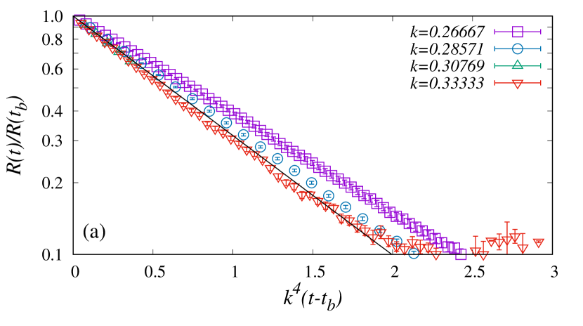
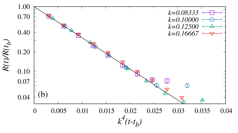
We can check however if the continuum prediction is upheld after the melting process with a simple scaling collapse. We first define a time ${t^{\prime}}=0$, which is taken to be the well after the beginning of the melting process, as the time at which $R(t)$ drops below a threshold of $0.01$ (chosen just for the convenience of analysis, once again we checked that this value only plays a quantitative role). We can now attempt a parameter free scaling collapse of $R({t^{\prime}})$ and would expect to get a linear profile on a log-linear plot for a range of $k$ by scaling the ${t^{\prime}}\to k^{4}{t^{\prime}}$. We present this analysis in Fig. 10 for $A=1.0$ and find a reasonable agreement with the expectation developed above, even if not entirely satisfactory. To further check the applicability of the continuum theory, we also consider ring exchange dynamics over $2\times 1$ plaquettes, which we expect to the same Eq. (3), but have much short pre-thermal times (as naturally be expected from a longer-range type of exchange). This allows to probe a larger range of wave-vectors $k$ values, as presented in Fig. 10 where the adherence to a $k^{4}{t^{\prime}}$ is clearly improved.

Figure 10: $R(t)$ scaled by the value closest to $0.01$ ($R(t_{b})$) in our dataset vs $k^{4}t^{\prime}$ where $t^{\prime}=t-t_{b}$ is the time shifted by the reference time $t_{b}$,for different values of $k$. A log-linear scale is chosen to emphasize the expected scaling in $k$ for different values of $k$. (a) : For the main ring-exchange model discussed in the manuscript. (b) Similar scaling for an extended model where we allow ring-exchanges models around $2\times 1$ and $1\times 2$ plaquettes.

V Pattern of dynamical activity in prethermal and melting process

Figure 11: (a) A sample initial configuration for an $80\times 80$ lattice with $k=0.05$ and $A=0.6$. Intersection of axes indicates origin. (b-d) Flippability correlator $C(x,y,t)$ for the same system size, averaged over $80$ initial conditions and $128$ realizations of the dynamics for each, at times (left to right) $t=2^{17},2^{19},2^{21}$.

The previous section shows that a mean field treatment is unable to recreate the slow dynamics seen numerically, thus hinting at the presence of correlations which are neglected at a mean field level. To understand the large-scale mechanisms involved in the prolongation of the prethermal lifetime and the onset of melting, we consider the build up and correlations of flippable plaquettes. This serves as a proxy for identifying dynamically active regions and their evolution. We study real-space flippability correlations through the normalized connected correlator

$$C(x,y,t)=\frac{\braket{P(0,0,t)P(x,y,t)}-\braket{P(0,0,t)}\braket{P(x,y,t)}}{\braket{P(t)}^{2}},$$

where $P(x,y,t)=1$ if the plaquette whose left bottom site is $(x,y)$ is flippable and zero otherwise, and $P(t)$ is the spatially averaged density of flippable plaquettes. Large (low) values of $C(x,y)$ at a given time will thus indicate strong (weak) correlations of flippability with the initial point. Recall that we have chosen starting configurations from annealing to a potential which is only a function of the tilted coordinate $x+y$. This means that we have a freedom of choosing the origin for our correlation function at any $x-y$ for fixed $x+y$. We take advantage of this symmetry by averaging over all equivalent positions of the origin. For the $x+y$ position of the origin we use our potential function as defined in Eq. (6) and set our origin to be the point satisfying $\vec{k}\cdot\vec{r}=\pi/4$. We make this choice as it lies at the threshold between highly active and inactive regions, defined by $\braket{n}=1/2$ (medium boson density, high density of flippable plaquettes) and $\braket{n}=1$ (high boson density, low density of flippable plaquettes).

Figure 12: (a) A sample filled-staggered-unfilled-staggered type initial configuration, as described in the main text, with $W=13$ consecutive diagonals filled. (b) $R(t)$ at the dominant wave-vector for various values of $W$, against rescaled time $k^{4}t$. (c) Flippability correlator $C(x,y,t)$ for configuration in (1) at $t=2^{23}$ (d) $C(x,y,t)$ for $W=27$ at $t=2^{21}$ with the same conditions. (e) Same as plot for $W=27$, scaled instead by $\langle P_{d_{i}}\rangle\langle P_{d_{j}}\rangle$.

V.1 Density wave patterns

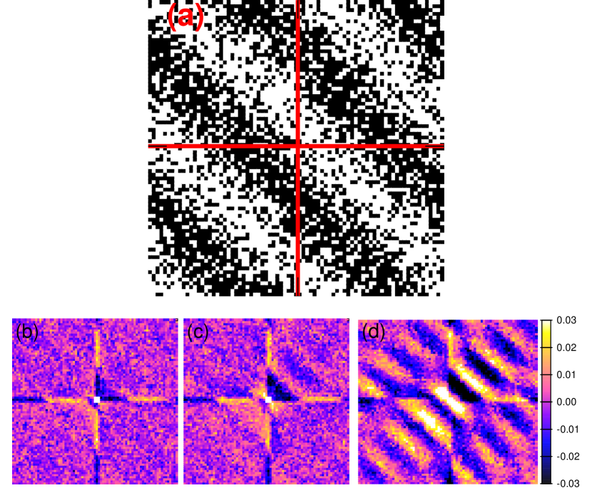
We begin by considering the initial conditions studied in the previous sections. To ensure that we are able to observe large scale (slowly varying spatial) features in the correlation function, we choose a system size of $80\times 80$ and $k=0.05$ at $A=0.6$ (a particular realization of this is shown in Fig. 11). To gather high quality statistics we average over 80 realizations for the initial condition and for each realization we run 128 realizations of the stochastic dynamics. The time $t_{0}$, which denotes the beginning of the melting process, is $\approx 10^{5}$ or $2^{17}$ for $k=0.05$, as seen in Fig. 9. We study $C(x,y,t)$ up to time scales of $2^{21}$ and find that strong anti-correlations develop at short range for the density of flippable plaquettes at early times, and sustain until the intermediate stages of melting. This is shown in Fig. 11, where snapshots of $C(x,y,t)$ at $t=2^{17}\to 2^{21}$ are presented.

This profile shows the development of active regions (bright) surrounded by inactive regions (dark), and suggests that a mechanism of excluded dynamical regions may be the source of dynamical slowing down. Note also that Fig. 11 suggests a bias of the dynamics towards the $x$ and $y$ axes, which may be expected from the continuum theory as well, due to the lack of radial symmetry. We see that even before the melting time, weak correlations are already built up along the $x$ and $y$ axes, but in a manner which is anti-correlated and modulated with the approximate stripe width. We find that this pattern begins to appear at times as short as $t=2^{4}=16$, but we present data at the last possible time value before melting which we have recorded as the pattern is visible with significantly more clarity.

Another important aspect of the correlation pattern to note here is the dependence on the $x-y$ coordinate (“perpendicular” to the initial wave-pattern), which is not built in in the initial condition as the energy used in the annealing process used to generate the configuration has no $x-y$ dependence. This behavior cannot also be expected from the continuum theory since we start of with a single wave like configuration with $k_{x}=k_{y}$.

We find that an important condition for the existence of such correlation patterns is that they are specific values of $A$ where the dynamics is not described by simple sub-diffusion. For example, we studied the case of $k=0.05$ at $A=0.2$, which shows conventional dynamics (as far as we can see from Fig. 9), and did not find any non-trivial correlations down to a precision of $10^{-4}$ in $C(x,y,t)$. This is as expected from a mean-field treatment, as it forbids correlations by definition.

The evolution of the correlation landscape for the duration of the melting process presented in Fig. 11 suggests that it proceeds through a merging of dynamically active regions. This will be discussed in more detail for step-like initial conditions, where a complete melting process can be observed with higher clarity and on longer times.

V.2 Maximally active square wave initial conditions

To gain a better understanding of the melting process, we begin with a more artificial initial condition chosen to have regions of flippable plaquettes with maximal and minimal density. We consider alternating patterns such as the one shown in Fig. 12, with $W$ (necessarily odd) consecutive diagonals filled, followed by $W+1$ in a perfect staggered (“Néel”) pattern, followed by $W$ empty diagonals, and finally by another $W+1$ in a Néel pattern to close out one period. These constraints are chosen to ensure that a filled region is bounded by empty diagonals and vice versa. The lattice size is then $N(2W+2(W+1))$, where $N$ is the number of periods. Although these configurations show melting times (quantified by the decay of the appropriate Fourier component) which are faster than those studied above, they show a scaling fore pre-melting which is slower than the conventional $k^{-4}$, as seen in Fig.11. We find that the flippability correlator $C(x,y,t)$ for these unconventional initial conditions shows an extension of the anti-correlated pattern in the $x-y$ direction with a periodic modulation across distances large compared to lattice spacing. This is seen clearly for $W=13$ with $N=2$ at time of $t=2^{23}=8\times 10^{6}$ in Fig. 12.

Figure 13: (a) $R(t)$ for $W=7$ and 2 stripes with vertical lines marking the times (b-f) $[4,6,8,11,14]\times 2^{20}$ for which $C(x,y,t)$ profiles are collected.

An important characteristic of the pattern described above is the value of the wave-vector associated to this pattern. We find that this is determined by the approximate stripe width, i.e. the wavelength $1/k$. Our data suggest that this occurs due to a development of the correlation along the $x$ and $y$ axes, which is limited by the size of active regions (high density of flippable plaquettes). Growth of correlation within an active region is mediated by alternating patterns of correlation and anti-correlation, which can be thought of as being generated by reflections off of the boundary between active and inactive regions, as shown in Fig. 12. Repeated reflections create the observed periodic pattern, thus linking the periodicity and the width of the initial stripes. This is clearly seen in the approximate periodicities of the pattern for $W=13$ and $27$ in Fig. 12 where the profiles look similar even though the stripe width is changed by a factor of 2. Strong signatures of the periodic pattern for stripe widths (or alternatively wavelengths) of $13$ and $27$ at approximately the same time indicates the emergence of this pattern at a time scale which only weakly depends on the wave-vector $k$, and that it develops at a time scale parametrically much smaller than the melting time. Note that an extrapolation based on Fig.11b indicates the beginning of melting to occur earliest at $t\approx 2^{27}$, assuming a lower bound of the scaling behavior as $k^{-4}$ (which is clearly slower than the scaling our numerics show in Fig.11b).

To develop an estimate of the relevance of this patterning to the process of melting, we first remove the normalization of $\braket{P(t)}$ which we have absorbed into the definition and instead look at $C(x,y,t)$ scaled by $\langle P_{d_{i}}(t)\rangle\langle P_{d_{j}}(t)\rangle$, where $\braket{P_{d_{i}}(t)}$ is the average number of flippable plaquettes in diagonal number $i$ at time $t$. This makes the correlation function effectively lie between $-1$ and $1$, with either limit describing a saturation to the largest (smallest) values. In particular, a value of $-1$ implies that the density of flippable plaquettes is zero, leading to a complete arrest of the dynamics. This version of $C(x,y,t)$ is plotted in Fig. 12e and we see clearly that close to the frontier of dynamical activity, we do get a complete anti-correlation around the reference region. This suggests that the dynamical activity is likely strongly controlled by the unconventional pattern in the $x-y$ direction.

Now we turn to an investigation of the role of the periodic patterns observed above in the melting process. We can study this by choosing a small enough $W$ so that the melting process is captured within the time scale of $10^{9}$ which we can simulate. We find that for $W=7$, the ratio $R(t)$ begins to deviate from unity at a time $t_{0}\sim 2^{21}=2\times 10^{6}$, and reaches a value of 0.01 by $t_{b}\sim 2^{24}=1.6\times 10^{7}$ (data plotted in Fig. 13). In this interval, we find at time $t=2^{20}$ a formation of stable periodic structures in the $x-y$ direction, and see a connection of the dynamically active regions for $t=2^{22}$. Finally by $t=2^{24}$, the correlation pattern has relaxed into a single wave in the $x+y$ direction, restoring the symmetry in the $x-y$ direction expected from the continuum prediction. The role of correlations is expected to be insignificant past this time point.

VI Summary and outlook

We studied a system of hard-core bosons on a square lattice evolving under classical stochastic dynamics using ring exchanges. We find that boson density waves motivated by the patterns present in the Hilbert space fragmentation of this model approach equilibrium on an extremely long time scale, which diverges with the inverse wave-vector as $k^{-\alpha}$ for small $k$, where $\alpha$ depends on the amplitude $A$ of the initial density wave configuration. For decreasing values of $A$, we find increasingly larger windows in the large $k$ regime where we observe a scaling of $k^{-4}$. Our numerical studies and mean-field treatments of simplified models show the emergence of sub-diffusion on the other-hand in the hydrodynamic low $k$ limit. For the hard-core case, we derive a dynamical equation using a mean-field like assumption which is able to capture partially the unconventional feature of an increase in slope around the nodes of the pattern driven by the non-linear terms in the dynamical equation but which also predicts a time scaling of $k^{-4}$. This leads us to the conclusion that the microscopic dynamics are controlled by strong correlations which are built up in the prethermal regime, which cannot be accounted for by this mean-field treatment.

To understand the mechanism driving the long prethermal regime, we study the correlation function of flippable plaquette density for different instances in time. We find that a strong anti-correlation is built up in the direction orthogonal to the modulation direction for the initial condition, even extending to the entire length of the diagonals for intermediate system sizes. We thus observe the formation of isolated dynamical puddles and find that the mechanism leading to the melting is characterized by a merger of these puddles, which relax into a profile which is consistent with what we expect from the continuum theory. Thus, we have found an example where correlations control crucial aspects of the dynamical behavior, and a simple mean-field like hydrodynamic description is insufficient. An important question remains: how generic are the long melting processes that we observe, in particular to which additional classes of initial conditions and types of dynamics do they apply? From the discussion of perfect stripe configurations presented in Sec. II, it is easy to see that similar results can also be expected for stripes which have a different tilt, as long as $k_{x},k_{y}\neq 0$. Regarding the possible set of dynamics which can be expected to engineer a similar phenomenology, we observe that a restricted spread of excitations similar to fractonic systems Nandkishore and Hermele (2019) may be at play here. For the specific model we study here this can be seen by considering the example discussed in Sec. II, where we see that the plaquette excitation is not able to move freely in the direction where there is a lack of similar excitations. More complex versions of this example can be generated by other spatially-larger dynamical terms conserving dipole moment, and can be expected to have a similar constraint when diffusing into spatial regions which lack dynamically active cells. This mechanism is nevertheless not as cleanly formulated and generic as the ones found in fractonic models Nandkishore and Hermele (2019); Chamon (2005); Pretko (2018). In particular it is still possible to define special particle configurations in our model, in which an active plaquette can move locally without restriction. However, our numerical results and the intuition developed in Sec. II suggest that for modulated structures which vary over large length scales, the phenomenology which we have discussed should hold for generic dipole moment conserving local dynamics.

We have shown that the decay of the overlap with the initial state with time shows a similar behavior upon comparing the exact quantum dynamics and our classical automaton for a small system size. This leads us to speculate that the behavior studied in the automaton language might inherit properties which can also be relevant for the exact quantum evolution for long times, as already seen for the study of sub-diffusive behavior in 1D Feldmeier et al. (2020). First of all, we expect that our hydrodynamic description might be equally valid also for the quantum dynamics, in case the quantum system exhibits a hydrodynamic long-time behavior. This would imply sub-diffusion also in the quantum case. Further, it might be possible that the onset of hydrodynamic behavior also in the quantum model might be delayed to very long times. This would have the consequence that a large intermediate time window exists with unconventionally slow dynamics. As this model is related to the quantum link model Karpov et al. (2021) via a relaxation of charge conservationKhudorozhkov et al. (2021), similar physics may be expected to emerge there in a more restricted setting. The category of initial conditions which we have studied may be seen as high energy states of a quantum XY model with ring exchange interactions Sandvik et al. (2002). We expect that an initial state with a fully staggered charge density pattern, located at low-energies for such a model with large ring-exchange, would relax extremely quickly as it has the maximal possible density of flippable plaquettes by the ring-exchange term.

Given that the stripe configurations we consider are qualitatively similar to domain walls in some ferromagnetic systems (such as found e.g. in Ising models Spirin et al. (2001)), it is important to note that the stability of domain walls in such cases is ensured by energetic reasons and is only expected at low temperature. In contrast, we do not have any such potential term which reinforces local correlations, and our long lived stripe structures are generated purely by the restricted dynamics available to the system.

The crossover between Hilbert space fragmentation, which dictates preservation of the memory of the initial state to arbitrarily long times, and the long prethermal plateaus we see here, is another promising direction in which investigations can be carried out to better our understanding of the processes involved. Although we do not find any exact conserved quantities which could explain the slow relaxation seen in our dipole conserving model, another interesting follow-up would be to try to build a theoretical framework in terms of statistically localized integrals of motion Rakovszky et al. (2020).

Finally, the rapid increase of the lifetime of the prethermal behavior with inverse wave-vector suggests that rare events, which create configurations allowing the applicability of the hydrodynamic theory, play a key role. An improved understanding of the potentially large deviations which lead to the above mentioned phenomenon would help greatly in developing a coarse-grained description of the dynamics at the threshold between the prethermal and equilibrium regimes.

Appendix A Low energy behavior of random configurations

Figure 14: $C(\vec{k},t)$ normalized by $C(\vec{0},t)$ for times $t=2^{12}$ (a) and $2^{16}$ (b).

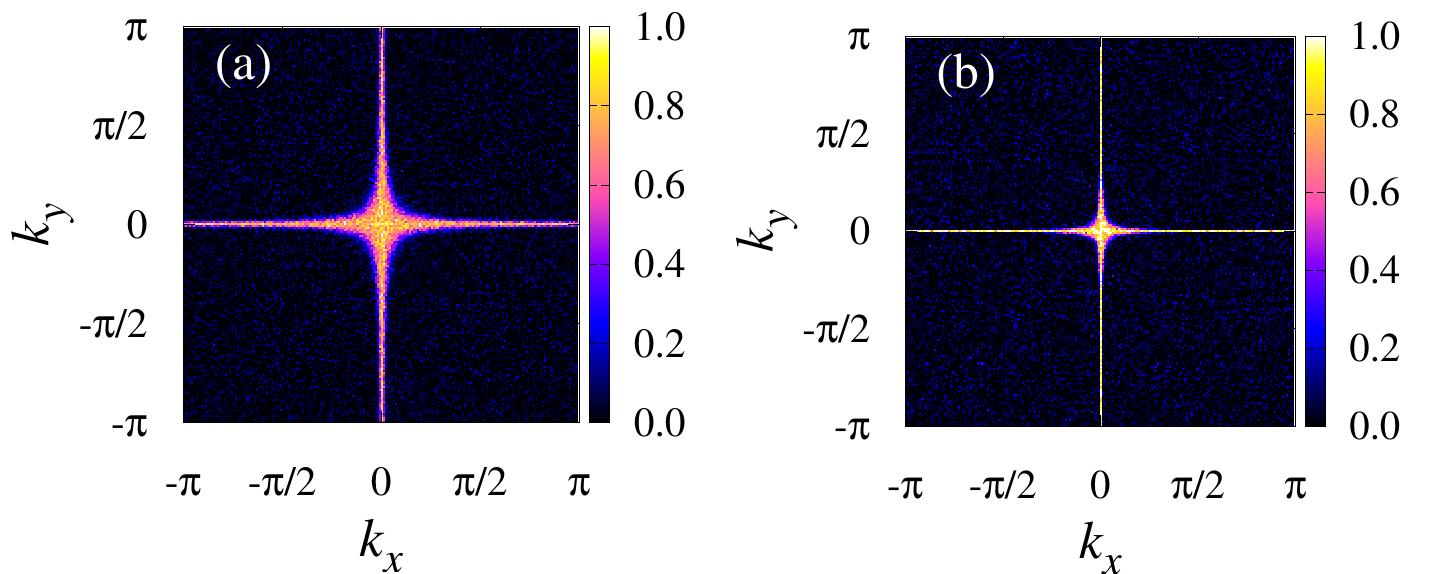
Here we follow the analysis developed in Ref. Sala et al. (2021) for a similar stochastic model. The authors consider a classical automaton on a square lattice which also conserves the dipole moment similar to the model we have considered. The microscopic dynamics is considered from the perspective of the long time correlation function, defined as $C(\vec{r},t)=\braket{n_{\vec{r}}(t)n_{0}(0)}$, where the expectation value is over random initial conditions and realizations of stochastic dynamics. The authors of Ref. Sala et al. (2021) estimate the correlation function in momentum space ($C(\vec{k},t)$) for a time much larger than the scale of the microscopic dynamics (using both automaton dynamics and an effective analytical ansatz) and find sub-diffusive features with “hidden” modulated symmetries corresponding to certain patterns in the Brillouin zone (see Fig.2b of Ref. Sala et al. (2021)).

In this appendix, we would like to check if this analysis can help identify the slow dynamics we observe for large scale modulated patterns. The energy spectrum as a function of $\vec{k}$ has already been identified in a mean-field framework by Paramekanti et al. in Ref. Paramekanti et al. (2002) for the form of ring-exchange used in our work, to be given by $E_{\vec{k}}\propto|\sin(k_{x}/2)\sin(k_{y}/2)|$. This trivially implies that the lines $k_{x}=0$ and $k_{y}=0$ host zero modes, and that this should be visible in $C(\vec{k},t)$ in the long time limit. Note that this profile does not explain the slow dynamics which we have explored in this work, as that would at the minimum require the presence of slow modes along tilted directions such as $k_{x}=k_{y}$. To check if this expectation is borne out by ring-exchange dynamics, we perform numerical evolutions of random configurations of a $200\times 200$ lattice for $t=2^{12}$ and $2^{16}$, shown in Fig. 14. We can clearly see that the profile is consistent with non-zero values being present only along the lines $k_{x}=0$ and $k_{y}=0$ at long times. This aspect of the dynamics is consistent with the mean-field treatment developed in the body of the manuscript. This is to be expected since random configurations correspond to the $A\to 0$ limit of our study of modulated patterns, which was shown to be well-described by the “vanilla” mean-field dynamics.

References

- Calabrese (2018) P. Calabrese, Physica A: Statistical Mechanics and its Applications 504, 31 (2018).
- Garrahan (2018) J. P. Garrahan, Physica A: Statistical Mechanics and its Applications 504, 130 (2018).
- Gogolin and Eisert (2016) C. Gogolin and J. Eisert, Reports on Progress in Physics 79, 056001 (2016).
- Browaeys and Lahaye (2020) A. Browaeys and T. Lahaye, Nature Physics 16, 132 (2020).
- Gross and Bloch (2017) C. Gross and I. Bloch, Science 357, 995 (2017).
- Abanin et al. (2019) D. A. Abanin, E. Altman, I. Bloch, and M. Serbyn, Rev. Mod. Phys. 91, 021001 (2019).
- Alet and Laflorencie (2018) F. Alet and N. Laflorencie, Comptes Rendus Physique 19, 498 (2018).
- Abanin and Papić (2017) D. A. Abanin and Z. Papić, Annalen der Physik 529, 1700169 (2017).
- Luitz et al. (2015) D. J. Luitz, N. Laflorencie, and F. Alet, Physical Review B 91, 081103(R) (2015).
- Sala et al. (2020) P. Sala, T. Rakovszky, R. Verresen, M. Knap, and F. Pollmann, Physical Review X 10, 011047 (2020).
- Khemani et al. (2020) V. Khemani, M. Hermele, and R. Nandkishore, Phys. Rev. B 101, 174204 (2020).
- Moudgalya et al. (2021) S. Moudgalya, B. A. Bernevig, and N. Regnault, arXiv preprint arXiv:2109.00548 (2021).
- Yang et al. (2020) Z.-C. Yang, F. Liu, A. V. Gorshkov, and T. Iadecola, Physical review letters 124, 207602 (2020).
- Mukherjee et al. (2021) B. Mukherjee, D. Banerjee, K. Sengupta, and A. Sen, Physical Review B 104, 155117 (2021).
- Karpov et al. (2021) P. Karpov, R. Verdel, Y.-P. Huang, M. Schmitt, and M. Heyl, Physical Review Letters 126, 130401 (2021).
- Zhang and Røising (2022) Z. Zhang and H. S. Røising, arXiv preprint arXiv:2206.01758 (2022).
- Sikora et al. (2011) O. Sikora, N. Shannon, F. Pollmann, K. Penc, and P. Fulde, Physical Review B 84, 115129 (2011).
- Ilievski et al. (2018) E. Ilievski, J. De Nardis, M. Medenjak, and T. Prosen, Physical review letters 121, 230602 (2018).
- McRoberts et al. (2022) A. J. McRoberts, T. Bilitewski, M. Haque, and R. Moessner, Physical Review B 105, L100403 (2022).
- Scheie et al. (2021) A. Scheie, N. Sherman, M. Dupont, S. Nagler, M. Stone, G. Granroth, J. Moore, and D. Tennant, Nature Physics 17, 726 (2021).
- Weiner et al. (2020) F. Weiner, P. Schmitteckert, S. Bera, and F. Evers, Physical Review B 101, 045115 (2020).
- Kardar et al. (1986) M. Kardar, G. Parisi, and Y.-C. Zhang, Physical Review Letters 56, 889 (1986).
- Iaconis et al. (2019) J. Iaconis, S. Vijay, and R. Nandkishore, Physical Review B 100, 214301 (2019).
- Feldmeier et al. (2020) J. Feldmeier, P. Sala, G. De Tomasi, F. Pollmann, and M. Knap, Physical Review Letters 125, 245303 (2020).
- Morningstar et al. (2020) A. Morningstar, V. Khemani, and D. A. Huse, Physical Review B 101, 214205 (2020).
- Iaconis et al. (2021) J. Iaconis, A. Lucas, and R. Nandkishore, Physical Review E 103, 022142 (2021).
- Richter and Pal (2022) J. Richter and A. Pal, Physical Review Research 4, L012003 (2022).
- Gromov et al. (2020) A. Gromov, A. Lucas, and R. M. Nandkishore, Physical Review Research 2, 033124 (2020).
- Nandkishore and Hermele (2019) R. M. Nandkishore and M. Hermele, Annual Review of Condensed Matter Physics 10, 295 (2019).
- Pretko et al. (2020) M. Pretko, X. Chen, and Y. You, International Journal of Modern Physics A 35, 2030003 (2020).
- Guardado-Sanchez et al. (2020) E. Guardado-Sanchez, A. Morningstar, B. M. Spar, P. T. Brown, D. A. Huse, and W. S. Bakr, Phys. Rev. X 10, 011042 (2020).
- Scherg et al. (2021) S. Scherg, T. Kohlert, P. Sala, F. Pollmann, B. Hebbe Madhusudhana, I. Bloch, and M. Aidelsburger, Nature Communications 12, 4490 (2021).
- Kohlert et al. (2021) T. Kohlert, S. Scherg, P. Sala, F. Pollmann, B. Hebbe Madhusudhana, I. Bloch, and M. Aidelsburger, arXiv e-prints , arXiv:2106.15586 (2021), arXiv:2106.15586 .
- Baiardi and Reiher (2019) A. Baiardi and M. Reiher, Journal of chemical theory and computation 15, 3481 (2019).
- Schmitt and Heyl (2020) M. Schmitt and M. Heyl, Physical Review Letters 125, 100503 (2020).
- Iadecola and Vijay (2020) T. Iadecola and S. Vijay, Physical Review B 102, 180302(R) (2020).
- Gopalakrishnan and Zakirov (2018) S. Gopalakrishnan and B. Zakirov, Quantum Science and Technology 3, 044004 (2018).
- Iaconis (2021) J. Iaconis, PRX Quantum 2, 010329 (2021).
- Nahum et al. (2017) A. Nahum, J. Ruhman, S. Vijay, and J. Haah, Phys. Rev. X 7, 031016 (2017).
- Gopalakrishnan (2018) S. Gopalakrishnan, Physical Review B 98, 060302(R) (2018).
- Castro-Alvaredo et al. (2016) O. A. Castro-Alvaredo, B. Doyon, and T. Yoshimura, Physical Review X 6, 041065 (2016).
- Bertini et al. (2016) B. Bertini, M. Collura, J. De Nardis, and M. Fagotti, Physical review letters 117, 207201 (2016).
- Klobas et al. (2021) K. Klobas, B. Bertini, and L. Piroli, Physical Review Letters 126, 160602 (2021).
- Alba et al. (2019) V. Alba, J. Dubail, and M. Medenjak, Physical review letters 122, 250603 (2019).
- Paramekanti et al. (2002) A. Paramekanti, L. Balents, and M. P. A. Fisher, Physical Review B 66, 054526 (2002).
- Rousseau et al. (2005) V. G. Rousseau, R. T. Scalettar, and G. G. Batrouni, Physical Review B 72, 054524 (2005).
- Schaffer et al. (2009) R. Schaffer, A. A. Burkov, and R. G. Melko, Physical Review B 80, 014503 (2009).
- Tay and Motrunich (2010) T. Tay and O. I. Motrunich, Physical review letters 105, 187202 (2010).
- Tay et al. (2011) T. Tay, O. I. Motrunich, et al., Physical Review B 83, 205107 (2011).
- Khudorozhkov et al. (2021) A. Khudorozhkov, A. Tiwari, C. Chamon, and T. Neupert, arXiv preprint arXiv:2107.09690 (2021).
- Sala et al. (2021) P. Sala, J. Lehmann, T. Rakovszky, and F. Pollmann, arXiv preprint arXiv:2110.08302 (2021).
- Canfield and McKay (2005) E. Canfield and B. McKay, Electronic Journal Of Combinatorics 12 (2005).
- Chamon (2005) C. Chamon, Physical review letters 94, 040402 (2005).
- Pretko (2018) M. Pretko, Physical Review B 98, 115134 (2018).
- Sandvik et al. (2002) A. W. Sandvik, S. Daul, R. R. P. Singh, and D. J. Scalapino, Physical review letters 89, 247201 (2002).
- Spirin et al. (2001) V. Spirin, P. L. Krapivsky, and S. Redner, Physical Review E 65, 016119 (2001).
- Rakovszky et al. (2020) T. Rakovszky, P. Sala, R. Verresen, M. Knap, and F. Pollmann, Physical Review B 101, 125126 (2020).