Robust and Fast Measure of Information via Low-rank Representation

Yuxin Dong1,2, Tieliang Gong1,2, Shujian Yu3, Hong Chen4,5, Chen Li1,2 Corresponding author.
Abstract

The matrix-based Rényi’s entropy allows us to directly quantify information measures from given data, without explicit estimation of the underlying probability distribution. This intriguing property makes it widely applied in statistical inference and machine learning tasks. However, this information theoretical quantity is not robust against noise in the data, and is computationally prohibitive in large-scale applications. To address these issues, we propose a novel measure of information, termed low-rank matrix-based Rényi’s entropy, based on low-rank representations of infinitely divisible kernel matrices. The proposed entropy functional inherits the specialty of of the original definition to directly quantify information from data, but enjoys additional advantages including robustness and effective calculation. Specifically, our low-rank variant is more sensitive to informative perturbations induced by changes in underlying distributions, while being insensitive to uninformative ones caused by noises. Moreover, low-rank Rényi’s entropy can be efficiently approximated by random projection and Lanczos iteration techniques, reducing the overall complexity from 𝒪(n3)𝒪superscript𝑛3\mathcal{O}(n^{3}) to 𝒪(n2s)𝒪superscript𝑛2𝑠\mathcal{O}(n^{2}s) or even 𝒪(ns2)𝒪𝑛superscript𝑠2\mathcal{O}(ns^{2}), where n𝑛n is the number of data samples and snmuch-less-than𝑠𝑛s\ll n. We conduct large-scale experiments to evaluate the effectiveness of this new information measure, demonstrating superior results compared to matrix-based Rényi’s entropy in terms of both performance and computational efficiency.

Introduction

The practical applications of traditional entropy measures e.g. Shannon’s entropy (Shannon 1948) and Rényi’s entropy (Rényi 1961) have long been hindered by their heavy reliance on the underlying data distributions, which are extremely hard to estimate or even intractable in high-dimensional spaces (Fan and Li 2006). Alternatively, the matrix-based Rényi’s entropy proposed by (Sanchez Giraldo, Rao, and Principe 2014) treats the entire eigenspectrum of a normalized kernel matrix as a probability distribution, thus allows direct quantification from given data samples by projecting them in reproducing kernel Hilbert spaces (RKHS) without the exhausting density estimation. This intriguing property makes matrix-based Rényi’s entropy and its multivariate extensions (Yu et al. 2019) successfully applied in various data science applications, ranging from classical dimensionality reduction and feature selection (Brockmeier et al. 2017; Álvarez-Meza et al. 2017) problems to advanced deep learning problems such as network pruning (Sarvani et al. 2021) and knowledge distillation (Miles, Rodríguez, and Mikolajczyk 2021).

Despite the empirical success of matrix-based Rényi’s entropy, it has been shown to be not robust against noises in the data (Yu et al. 2019), because it cannot distinguish them from linear combinations of informative features in high-dimensional scenarios. Moreover, the exact calculation requires 𝒪(n3)𝒪superscript𝑛3\mathcal{O}(n^{3}) time complexity with traditional eigenvalue decomposition techniques e.g. CUR decomposition and QR factorization (Mahoney and Drineas 2009; Watkins 2008), greatly hampering its application in large scale tasks due to the unacceptable computational cost.

Inspired by the success of min-entropy which uses the largest outcome solely as a measure of information (Wan et al. 2018; Konig, Renner, and Schaffner 2009), we seek for a robust information quantity by utilizing low-rank representations of kernel matrices. Our new definition, termed low-rank matrix-based Rényi’s entropy (abbreviated as low-rank Rényi’s entropy), fulfills the entire set of axioms provided by Rényi (Rényi 1961) that a function must satisfy to be considered a measure of information. Compared to the original matrix-based Rényi’s entropy, our low-rank variant is more sensitive to informative perturbations caused by variation of the underlying probability distribution, while being more robust to uninformative ones caused by noises in the data samples. Moreover, our low-rank Rényi’s entropy can be efficiently approximated by random projection and Lanczos iteration techniques, achieving substantially lower time complexity than the trivial eigenvalue decomposition approach. We theoretically analyze the quality of approximation results, and conduct large-scale experiments to evaluate the effectiveness of low-rank Rényi’s entropy as well as the approximation algorithms. The main contributions of this work are summarized as follows:

  • We extend Giraldo et al.’s definition and show that a measure of entropy can be built upon the low-rank representation of the kernel matrix. Our low-rank definition can be naturally extended to measure the interactions between multiple random variables, including joint entropy, conditional entropy, and mutual information.

  • Theoretically, we show that low-rank Rényi’s entropy is more insensitive to random perturbations of the data samples under mild assumptions. We also give empirical examples of low-rank Rényi’s entropy achieving higher discriminability for different eigenspectrum distributions through a proper choice of the hyper-parameter k𝑘k.

  • We develop efficient algorithms to approximate low-rank Rényi’s entropy through random projection and Lanczos iteration techniques, enabling fast and accurate estimations respectively. The overall complexity is reduced from 𝒪(n3)𝒪superscript𝑛3\mathcal{O}(n^{3}) to 𝒪(n2s)𝒪superscript𝑛2𝑠\mathcal{O}(n^{2}s) or even 𝒪(ns2)𝒪𝑛superscript𝑠2\mathcal{O}(ns^{2}) for some snmuch-less-than𝑠𝑛s\ll n, leading to a significant speedup compared to the original matrix-based Rényi’s entropy.

  • We evaluate the effectiveness of low-rank Rényi’s entropy on large-scale synthetic and real-world datasets, demonstrating superior performance compared to the original matrix-based Rényi’s entropy while bringing tremendous improvements in computational efficiency.

Related Work

Matrix-based Rényi’s Entropy

Given random variable 𝐗𝐗{\bf X} with probability density function (PDF) p(𝐱)𝑝𝐱p({\bf x}) defined in a finite set 𝒳𝒳\mathcal{X}, the α𝛼\alpha-order Rényi’s entropy (α>0,α1formulae-sequence𝛼0𝛼1\alpha>0,\alpha\neq 1) 𝐇α(𝐗)subscript𝐇𝛼𝐗{\bf H}_{\alpha}({\bf X}) is defined as

𝐇α(𝐗)=11αlog2𝒳pα(𝐱)d𝐱,subscript𝐇𝛼𝐗11𝛼subscript2subscript𝒳superscript𝑝𝛼𝐱differential-d𝐱\textstyle{\bf H}_{\alpha}({\bf X})=\frac{1}{1-\alpha}\log_{2}\int_{\mathcal{X}}p^{\alpha}({\bf x})\mathop{}\!\mathrm{d}{\bf x},

where the limit case α1𝛼1\alpha\rightarrow 1 yields the well-known Shannon’s entropy. It is easy to see that Rényi’s entropy relies heavily on the distribution of the underlying variable 𝐗𝐗{\bf X}, preventing its further adoption in data-driven science, especially for high-dimensional scenarios. To alleviate this issue, an alternative measure namely matrix-based Rényi’s entropy was proposed (Sanchez Giraldo, Rao, and Principe 2014):

Definition 1.

Let κ:𝒳×𝒳:𝜅maps-to𝒳𝒳\kappa:\mathcal{X}\times\mathcal{X}\mapsto\mathbb{R} be an infinitely divisible positive kernel (Bhatia 2006). Given {𝐱i}i=1n𝒳superscriptsubscriptsubscript𝐱𝑖𝑖1𝑛𝒳\{{\bf x}_{i}\}_{i=1}^{n}\subset\mathcal{X}, each 𝐱isubscript𝐱𝑖{\bf x}_{i} being a real-valued scalar or vector, and the Gram matrix K𝐾K obtained from Kij=κ(𝐱i,𝐱j)subscript𝐾𝑖𝑗𝜅subscript𝐱𝑖subscript𝐱𝑗K_{ij}=\kappa({\bf x}_{i},{\bf x}_{j}), a matrix-based analogue to Rényi’s α𝛼\alpha-entropy can be defined as:

𝐒α(𝐀)=11αlog2(i=1nλiα(𝐀)),subscript𝐒𝛼𝐀11𝛼subscript2superscriptsubscript𝑖1𝑛superscriptsubscript𝜆𝑖𝛼𝐀\textstyle{\bf S}_{\alpha}({\bf A})=\frac{1}{1-\alpha}\log_{2}\Big{(}\sum_{i=1}^{n}\lambda_{i}^{\alpha}({\bf A})\Big{)},

where 𝐀ij=1nKijKiiKjjsubscript𝐀𝑖𝑗1𝑛subscript𝐾𝑖𝑗subscript𝐾𝑖𝑖subscript𝐾𝑗𝑗{\bf A}_{ij}=\frac{1}{n}\frac{K_{ij}}{\sqrt{K_{ii}K_{jj}}} is a normalized kernel matrix and λi(𝐀)subscript𝜆𝑖𝐀\lambda_{i}({\bf A}) is the i𝑖i-th largest eigenvalue of 𝐀𝐀{\bf A}.

The kernel matrix 𝐀𝐀{\bf A} is positive semi-definite (PSD) and satisfies 𝐭𝐫(𝐀)=1𝐭𝐫𝐀1{\bf tr}({\bf A})=1, therefore λi[0,1]subscript𝜆𝑖01\lambda_{i}\in[0,1] for all i[1,n]𝑖1𝑛i\in[1,n]. With this setting, one can similarly define matrix notion of Rényi’s conditional entropy 𝐒α(𝐀|𝐁)subscript𝐒𝛼conditional𝐀𝐁{\bf S}_{\alpha}({\bf A}|{\bf B}), mutual information 𝐈α(𝐀;𝐁)subscript𝐈𝛼𝐀𝐁{\bf I}_{\alpha}({\bf A};{\bf B}), and their multivariate extensions (Yu et al. 2019).

Approximating Matrix-based Rényi’s Entropy

Exactly calculating 𝐒α(𝐀)subscript𝐒𝛼𝐀{\bf S}_{\alpha}({\bf A}) requires 𝒪(n3)𝒪superscript𝑛3\mathcal{O}(n^{3}) time complexity in general with traditional eigenvalue decomposition techniques. Recently, several attempts have been made towards accelerating the computation of 𝐒α(𝐀)subscript𝐒𝛼𝐀{\bf S}_{\alpha}({\bf A}) from the perspective of randomized numerical linear algebra (Gong et al. 2021; Dong et al. 2022). Although we also develop fast approximations, the motivation and technical solutions are totally different: we aim to propose a new measure of information that is robust to noise in data and also enjoys fast computation, whereas Gong and Dong et al. only accelerate the original matrix-based Rényi’s entropy. Moreover, in terms of adopted mathematical tools, we mainly focus on random projection and Lanczos iteration algorithms, rather than stochastic trace estimation and polynomial approximation techniques used in their works. As a result, the corresponding theoretical error bounds are also different.

A Low-rank Definition of Rényi’s Entropy

Our motivations root in two observations. Recall that the min-entropy (Konig, Renner, and Schaffner 2009), defined by 𝐇min(𝐗)=log2max𝐱𝒳p(𝐱)subscript𝐇min𝐗subscript2subscript𝐱𝒳𝑝𝐱{\bf H}_{\mathrm{min}}({\bf X})=-\log_{2}\max_{{\bf x}\in\mathcal{X}}p({\bf x}), measures the amount of information using solely the largest probability outcome. In terms of quantum statistical mechanics, it is the largest eigenvalue of the quantum state ρ𝜌\rho which is PSD and has unit trace (Ohya and Petz 2004). On the other hand, the eigenvalues with the maximum magnitude characterize the main properties of a PSD matrix. Inspired by these observations, we develop a robust information theoretical quantity by exploiting the low-rank representation:

Definition 2.

Let κ:𝒳×𝒳:𝜅maps-to𝒳𝒳\kappa:\mathcal{X}\times\mathcal{X}\mapsto\mathbb{R} be an infinitely divisible kernel. Given {𝐱i}i=1n𝒳superscriptsubscriptsubscript𝐱𝑖𝑖1𝑛𝒳\{{\bf x}_{i}\}_{i=1}^{n}\subset\mathcal{X} and integer k[1,n1]𝑘1𝑛1k\in[1,n-1], the low-rank Rényi’s α𝛼\alpha-order entropy is defined as:

𝐒αk(𝐀)=11αlog2(i=1kλiα(𝐀)+(nk)λrα(𝐀)),superscriptsubscript𝐒𝛼𝑘𝐀11𝛼subscript2superscriptsubscript𝑖1𝑘superscriptsubscript𝜆𝑖𝛼𝐀𝑛𝑘superscriptsubscript𝜆𝑟𝛼𝐀\textstyle{\bf S}_{\alpha}^{k}({\bf A})=\frac{1}{1-\alpha}\log_{2}\left\lparen\sum_{i=1}^{k}\lambda_{i}^{\alpha}({\bf A})+(n-k)\lambda_{r}^{\alpha}({\bf A})\right\rparen,

where 𝐀𝐀{\bf A} is the normalized kernel matrix constructed from {𝐱i}i=1nsuperscriptsubscriptsubscript𝐱𝑖𝑖1𝑛\{{\bf x}_{i}\}_{i=1}^{n} and κ𝜅\kappa, λi(𝐀)subscript𝜆𝑖𝐀\lambda_{i}({\bf A}) is the i𝑖i-th largest eigenvalues of 𝐀𝐀{\bf A} and λr(𝐀)=1nk(1i=1kλi(𝐀))subscript𝜆𝑟𝐀1𝑛𝑘1superscriptsubscript𝑖1𝑘subscript𝜆𝑖𝐀\lambda_{r}({\bf A})=\frac{1}{n-k}\big{(}1-\sum_{i=1}^{k}\lambda_{i}({\bf A})\big{)}.

Let 𝐀ksubscript𝐀𝑘{\bf A}_{k} be the best rank-k𝑘k approximation of 𝐀𝐀{\bf A} and Lk(𝐀)subscript𝐿𝑘𝐀L_{k}({\bf A}) be the matrix constructed by replacing the smaller nk𝑛𝑘n-k eigenvalues in 𝐀𝐀{\bf A} to λr(𝐀)subscript𝜆𝑟𝐀\lambda_{r}({\bf A}). It is easy to verify that 𝐒αk(𝐀)=𝐒αk(𝐀k)=𝐒αk(Lk(𝐀))=𝐒α(Lk(𝐀))superscriptsubscript𝐒𝛼𝑘𝐀superscriptsubscript𝐒𝛼𝑘subscript𝐀𝑘superscriptsubscript𝐒𝛼𝑘subscript𝐿𝑘𝐀subscript𝐒𝛼subscript𝐿𝑘𝐀{\bf S}_{\alpha}^{k}({\bf A})={\bf S}_{\alpha}^{k}({\bf A}_{k})={\bf S}_{\alpha}^{k}(L_{k}({\bf A}))={\bf S}_{\alpha}(L_{k}({\bf A})). Definition 2 complements the smaller eigenvalues through a uniform distribution, which is the unique method that fulfills all axioms below (the uniqueness is discussed in the appendix111https://github.com/Gamepiaynmo/LRMI).

Proposition 1.

Let 𝐀,𝐁n×n𝐀𝐁superscript𝑛𝑛{\bf A},{\bf B}\in\mathbb{R}^{n\times n} be arbitrary normalized kernel matrices, then

  1. (a)

    𝐒αk(𝐏𝐀𝐏)=𝐒αk(𝐀)superscriptsubscript𝐒𝛼𝑘superscript𝐏𝐀𝐏topsuperscriptsubscript𝐒𝛼𝑘𝐀{\bf S}_{\alpha}^{k}({\bf P}{\bf A}{\bf P}^{\top})={\bf S}_{\alpha}^{k}({\bf A}) for any orthogonal matrix 𝐏𝐏{\bf P}.

  2. (b)

    𝐒αk(p𝐀)superscriptsubscript𝐒𝛼𝑘𝑝𝐀{\bf S}_{\alpha}^{k}(p{\bf A}) is a continuous function for 0<p10𝑝10<p\leq 1.

  3. (c)

    0𝐒αk(𝐀)𝐒αk(1n𝐈)=log2(n)0superscriptsubscript𝐒𝛼𝑘𝐀superscriptsubscript𝐒𝛼𝑘1𝑛𝐈subscript2𝑛0\leq{\bf S}_{\alpha}^{k}({\bf A})\leq{\bf S}_{\alpha}^{k}(\frac{1}{n}{\bf I})=\log_{2}(n).

  4. (d)

    𝐒α2nkk2(Lk(𝐀)Lk(𝐁))=𝐒αk(𝐀)+𝐒αk(𝐁)superscriptsubscript𝐒𝛼2𝑛𝑘superscript𝑘2tensor-productsubscript𝐿𝑘𝐀subscript𝐿𝑘𝐁superscriptsubscript𝐒𝛼𝑘𝐀superscriptsubscript𝐒𝛼𝑘𝐁{\bf S}_{\alpha}^{2nk-k^{2}}\big{(}L_{k}({\bf A})\otimes L_{k}({\bf B})\big{)}={\bf S}_{\alpha}^{k}({\bf A})+{\bf S}_{\alpha}^{k}({\bf B}).

  5. (e)

    If 𝐀𝐁=𝐁𝐀=𝟎𝐀𝐁𝐁𝐀0{\bf A}{\bf B}={\bf B}{\bf A}=\mathbf{0} and 𝐭𝐫(𝐀k)=𝐭𝐫(𝐁k)=1𝐭𝐫subscript𝐀𝑘𝐭𝐫subscript𝐁𝑘1{\bf tr}({\bf A}_{k})={\bf tr}({\bf B}_{k})=1, then for g(x)=2(1α)x𝑔𝑥superscript21𝛼𝑥g(x)=2^{(1-\alpha)x} and t[0,1]𝑡01t\in[0,1], we have 𝐒α2k(t𝐀+(1t)𝐁)=g1(tg(𝐒αk(𝐀))+(1t)g(𝐒αk(𝐁)))superscriptsubscript𝐒𝛼2𝑘𝑡𝐀1𝑡𝐁superscript𝑔1𝑡𝑔superscriptsubscript𝐒𝛼𝑘𝐀1𝑡𝑔superscriptsubscript𝐒𝛼𝑘𝐁{\bf S}_{\alpha}^{2k}\big{(}t{\bf A}+(1-t){\bf B}\big{)}=g^{-1}\big{(}tg({\bf S}_{\alpha}^{k}({\bf A}))+(1-t)g({\bf S}_{\alpha}^{k}({\bf B}))\big{)}.

  6. (f)

    𝐒αk(𝐀𝐁𝐭𝐫(𝐀𝐁))max(𝐒αk(𝐀),𝐒αk(𝐁))superscriptsubscript𝐒𝛼𝑘𝐀𝐁𝐭𝐫𝐀𝐁superscriptsubscript𝐒𝛼𝑘𝐀superscriptsubscript𝐒𝛼𝑘𝐁{\bf S}_{\alpha}^{k}\left\lparen\frac{{\bf A}\circ{\bf B}}{{\bf tr}({\bf A}\circ{\bf B})}\right\rparen\geq\max\left\lparen{\bf S}_{\alpha}^{k}({\bf A}),{\bf S}_{\alpha}^{k}({\bf B})\right\rparen.

  7. (g)

    𝐒αk(𝐀𝐁𝐭𝐫(𝐀𝐁))𝐒αk(𝐀)+𝐒αk(𝐁)superscriptsubscript𝐒𝛼𝑘𝐀𝐁𝐭𝐫𝐀𝐁superscriptsubscript𝐒𝛼𝑘𝐀superscriptsubscript𝐒𝛼𝑘𝐁{\bf S}_{\alpha}^{k}\left\lparen\frac{{\bf A}\circ{\bf B}}{{\bf tr}({\bf A}\circ{\bf B})}\right\rparen\leq{\bf S}_{\alpha}^{k}({\bf A})+{\bf S}_{\alpha}^{k}({\bf B}).

Remark 1.

Proposition 1 characterizes the basic properties of low-rank Rényi’s entropy, in which (a)-(e) are the set of axioms provided by Rényi (Rényi 1961) that a function must satisfy to be a measure of information. Additionally, (f) and (g) together imply a definition of joint entropy which is also compatible with the individual entropy measures:

𝐒αk(𝐀,𝐁)=𝐒αk(𝐀𝐁𝐭𝐫(𝐀𝐁)).superscriptsubscript𝐒𝛼𝑘𝐀𝐁superscriptsubscript𝐒𝛼𝑘𝐀𝐁𝐭𝐫𝐀𝐁\textstyle{\bf S}_{\alpha}^{k}({\bf A},{\bf B})={\bf S}_{\alpha}^{k}\left\lparen\frac{{\bf A}\circ{\bf B}}{{\bf tr}({\bf A}\circ{\bf B})}\right\rparen.

This further allows us to define the low-rank conditional entropy 𝐒αk(𝐀|𝐁)superscriptsubscript𝐒𝛼𝑘conditional𝐀𝐁{\bf S}_{\alpha}^{k}({\bf A}|{\bf B}) and mutual information 𝐈αk(𝐀;𝐁)superscriptsubscript𝐈𝛼𝑘𝐀𝐁{\bf I}_{\alpha}^{k}({\bf A};{\bf B}), whose positiveness is guaranteed by (f) and (g) respectively:

𝐒αk(𝐀|𝐁)=𝐒αk(𝐀,𝐁)𝐒αk(𝐁),superscriptsubscript𝐒𝛼𝑘conditional𝐀𝐁superscriptsubscript𝐒𝛼𝑘𝐀𝐁superscriptsubscript𝐒𝛼𝑘𝐁\displaystyle{\bf S}_{\alpha}^{k}({\bf A}|{\bf B})={\bf S}_{\alpha}^{k}({\bf A},{\bf B})-{\bf S}_{\alpha}^{k}({\bf B}),
𝐈αk(𝐀;𝐁)=𝐒αk(𝐀)+𝐒αk(𝐁)𝐒αk(𝐀,𝐁).superscriptsubscript𝐈𝛼𝑘𝐀𝐁superscriptsubscript𝐒𝛼𝑘𝐀superscriptsubscript𝐒𝛼𝑘𝐁superscriptsubscript𝐒𝛼𝑘𝐀𝐁\displaystyle{\bf I}_{\alpha}^{k}({\bf A};{\bf B})={\bf S}_{\alpha}^{k}({\bf A})+{\bf S}_{\alpha}^{k}({\bf B})-{\bf S}_{\alpha}^{k}({\bf A},{\bf B}).

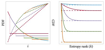
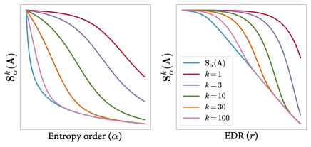
An intuitive overview of the comparative behavior between 𝐒α(𝐀)subscript𝐒𝛼𝐀{\bf S}_{\alpha}({\bf A}) and 𝐒αk(𝐀)superscriptsubscript𝐒𝛼𝑘𝐀{\bf S}_{\alpha}^{k}({\bf A}) for n=1000𝑛1000n=1000 is reported in Figure 1 and 2, where we evaluate the impact of k𝑘k, α𝛼\alpha and eigenspectrum decay rate (EDR) r𝑟r respectively. The eigenvalues are initialized by λi=eri/nsubscript𝜆𝑖superscript𝑒𝑟𝑖𝑛\lambda_{i}=e^{-ri/n} and then normalized. It can be observed from Figure 1 that 𝐒αk(𝐀)superscriptsubscript𝐒𝛼𝑘𝐀{\bf S}_{\alpha}^{k}({\bf A}) is always larger than 𝐒α(𝐀)subscript𝐒𝛼𝐀{\bf S}_{\alpha}({\bf A}) since the uncertainty of the latter nk𝑛𝑘n-k outcomes are maximized. Moreover, 𝐒αk(𝐀)superscriptsubscript𝐒𝛼𝑘𝐀{\bf S}_{\alpha}^{k}({\bf A}) quickly converges to 𝐒α(𝐀)subscript𝐒𝛼𝐀{\bf S}_{\alpha}({\bf A}) with the increase of k𝑘k, especially in extreme cases when the eigenspectrum of 𝐀𝐀{\bf A} is flat or steep. From Figure 2, we can see that for small k𝑘k, 𝐒αk(𝐀)superscriptsubscript𝐒𝛼𝑘𝐀{\bf S}_{\alpha}^{k}({\bf A}) decreases slow with the increase of α𝛼\alpha when α<1𝛼1\alpha<1 and fast otherwise. This behavior is the opposite when k𝑘k becomes large. Furthermore, we can see that EDR directly influences the value of entropy, as a flat eigenspectrum indicates higher uncertainty and steep the opposite. As can be seen, 𝐒αk(𝐀)superscriptsubscript𝐒𝛼𝑘𝐀{\bf S}_{\alpha}^{k}({\bf A}) monotonically decreases with the increase of r𝑟r, and decreases faster than 𝐒α(𝐀)subscript𝐒𝛼𝐀{\bf S}_{\alpha}({\bf A}) in a certain range which varies according to the choice of k𝑘k, indicating higher sensitivity to informative distribution changes when the hyper-parameter k𝑘k is selected properly.

Refer to caption
Figure 1: Left: PDF (solid) and CDF (dashed) of the altered eigenspectrum for different ranks k𝑘k. Right: The convergence behavior of 𝐒αk(𝐀)superscriptsubscript𝐒𝛼𝑘𝐀{\bf S}_{\alpha}^{k}({\bf A}) (solid) to 𝐒α(𝐀)subscript𝐒𝛼𝐀{\bf S}_{\alpha}({\bf A}) (dashed) with the increase of rank k𝑘k for different EDR (r𝑟r).

Moreover, consider the case that the data samples {𝐱i}i=1nsuperscriptsubscriptsubscript𝐱𝑖𝑖1𝑛\{{\bf x}_{i}\}_{i=1}^{n} are randomly perturbed, i.e. 𝐲i=𝐱i+ε𝐩isubscript𝐲𝑖subscript𝐱𝑖𝜀subscript𝐩𝑖{\bf y}_{i}={\bf x}_{i}+\varepsilon{\bf p}_{i}, where 𝐩isubscript𝐩𝑖{\bf p}_{i} are random vectors comprised of i.i.d. entries with zero expectation and unit variance. Let 𝐀𝐀{\bf A} and 𝐁𝐁{\bf B} be kernel matrices constructed from {𝐱i}i=1nsuperscriptsubscriptsubscript𝐱𝑖𝑖1𝑛\{{\bf x}_{i}\}_{i=1}^{n} and {𝐲i}i=1nsuperscriptsubscriptsubscript𝐲𝑖𝑖1𝑛\{{\bf y}_{i}\}_{i=1}^{n} respectively, and let {λi}i=1nsuperscriptsubscriptsubscript𝜆𝑖𝑖1𝑛\{\lambda_{i}\}_{i=1}^{n}, {μi}i=1nsuperscriptsubscriptsubscript𝜇𝑖𝑖1𝑛\{\mu_{i}\}_{i=1}^{n} be their eigenvalues. Then it satisfies that μiλi+𝐮i(𝐁𝐀)𝐮isubscript𝜇𝑖subscript𝜆𝑖superscriptsubscript𝐮𝑖top𝐁𝐀subscript𝐮𝑖\mu_{i}\approx\lambda_{i}+{\bf u}_{i}^{\top}({\bf B}-{\bf A}){\bf u}_{i} (Ngo 2005), where 𝐮isubscript𝐮𝑖{\bf u}_{i} is the corresponding eigenvector of λisubscript𝜆𝑖\lambda_{i}. When ε𝜀\varepsilon is small, the entries as well as the eigenvalues of 𝐀𝐀{\bf A} are nearly independently perturbed. The following theorem shows that 𝐒αk(𝐀)superscriptsubscript𝐒𝛼𝑘𝐀{\bf S}_{\alpha}^{k}({\bf A}) is more robust against small noises in data compared to 𝐒α(𝐀)subscript𝐒𝛼𝐀{\bf S}_{\alpha}({\bf A}):

Theorem 1.

Let {νi}i=1nsuperscriptsubscriptsubscript𝜈𝑖𝑖1𝑛\{\nu_{i}\}_{i=1}^{n} be independent random variables with zero mean and variance {σi2}i=1nsuperscriptsubscriptsuperscriptsubscript𝜎𝑖2𝑖1𝑛\{\sigma_{i}^{2}\}_{i=1}^{n}. Let 𝐀𝐀{\bf A} and 𝐁𝐁{\bf B} be PSD matrices with eigenvalues λisubscript𝜆𝑖\lambda_{i} and μi=λi+νisubscript𝜇𝑖subscript𝜆𝑖subscript𝜈𝑖\mu_{i}=\lambda_{i}+\nu_{i} respectively. If i=1kσi2i=k+1nσi2superscriptsubscript𝑖1𝑘superscriptsubscript𝜎𝑖2superscriptsubscript𝑖𝑘1𝑛superscriptsubscript𝜎𝑖2\sum_{i=1}^{k}\sigma_{i}^{2}\leq\sum_{i=k+1}^{n}\sigma_{i}^{2} or α>1𝛼1\alpha>1, there exists ϵ>0italic-ϵ0\epsilon>0 such that when all |νi|ϵsubscript𝜈𝑖italic-ϵ|\nu_{i}|\leq\epsilon, we have 𝐕𝐚𝐫[𝐈𝐏αk(𝐁)]𝐕𝐚𝐫[𝐈𝐏α(𝐁)]𝐕𝐚𝐫delimited-[]superscriptsubscript𝐈𝐏𝛼𝑘𝐁𝐕𝐚𝐫delimited-[]subscript𝐈𝐏𝛼𝐁{\bf Var}[{\bf IP}_{\alpha}^{k}({\bf B})]\leq{\bf Var}[{\bf IP}_{\alpha}({\bf B})], where 𝐈𝐏𝐈𝐏{\bf IP} is the information potential (Gokcay and Principe 2000) defined as 𝐈𝐏α(𝐁)=2(1α)𝐒α(𝐁)subscript𝐈𝐏𝛼𝐁superscript21𝛼subscript𝐒𝛼𝐁{\bf IP}_{\alpha}({\bf B})=2^{(1-\alpha){\bf S}_{\alpha}({\bf B})} and 𝐈𝐏αk(𝐁)=2(1α)𝐒αk(𝐁)superscriptsubscript𝐈𝐏𝛼𝑘𝐁superscript21𝛼superscriptsubscript𝐒𝛼𝑘𝐁{\bf IP}_{\alpha}^{k}({\bf B})=2^{(1-\alpha){\bf S}_{\alpha}^{k}({\bf B})}.

Remark 2.

Theorem 1 indicates that 𝐈𝐏αk(𝐁)superscriptsubscript𝐈𝐏𝛼𝑘𝐁{\bf IP}_{\alpha}^{k}({\bf B}) enables lower variance than 𝐈𝐏α(𝐁)subscript𝐈𝐏𝛼𝐁{\bf IP}_{\alpha}({\bf B}) against random perturbation of the eigenvalues under mild conditions, which is easy to be satisfied since in most cases we have knmuch-less-than𝑘𝑛k\ll n. Combining with our discussion above, the low-rank Rényi’s entropy is more sensitive to informative variations in probability distributions which will surely induce an increase or decrease in entropy, while being insensitive to uninformative perturbations caused by noises in the data samples.

Extending to Multivariate Scenarios

Following Definition 2 and Proposition 1, the low-rank variant of multivariate Rényi’s joint entropy, in virtue of the Venn diagram relation for Shannon’s entropy (Yeung 1991), could be naturally derived:

Definition 3.

Let {κi}i=1L:𝒳i×𝒳i:superscriptsubscriptsubscript𝜅𝑖𝑖1𝐿maps-tosuperscript𝒳𝑖superscript𝒳𝑖\{\kappa_{i}\}_{i=1}^{L}:\mathcal{X}^{i}\times\mathcal{X}^{i}\mapsto\mathbb{R} be positive infinitely divisible kernels and {𝐱i1,,𝐱iL}i=1n𝒳1××𝒳Lsuperscriptsubscriptsuperscriptsubscript𝐱𝑖1superscriptsubscript𝐱𝑖𝐿𝑖1𝑛superscript𝒳1superscript𝒳𝐿\{{\bf x}_{i}^{1},\cdots,{\bf x}_{i}^{L}\}_{i=1}^{n}\subset\mathcal{X}^{1}\times\cdots\times\mathcal{X}^{L}, the low-rank Rényi’s joint entropy is defined as:

𝐒αk(𝐀1,,𝐀L)=𝐒αk(𝐀1𝐀L𝐭𝐫(𝐀1𝐀L)),superscriptsubscript𝐒𝛼𝑘subscript𝐀1subscript𝐀𝐿superscriptsubscript𝐒𝛼𝑘subscript𝐀1subscript𝐀𝐿𝐭𝐫subscript𝐀1subscript𝐀𝐿\textstyle{\bf S}_{\alpha}^{k}({\bf A}_{1},\cdots,{\bf A}_{L})={\bf S}_{\alpha}^{k}\left\lparen\frac{{\bf A}_{1}\circ\cdots\circ{\bf A}_{L}}{\mathbf{tr}({\bf A}_{1}\circ\cdots\circ{\bf A}_{L})}\right\rparen,

where 𝐀1,,𝐀Lsubscript𝐀1subscript𝐀𝐿{\bf A}_{1},\cdots,{\bf A}_{L} are normalized kernel matrices constructed from {𝐱i1}i=1nsuperscriptsubscriptsuperscriptsubscript𝐱𝑖1𝑖1𝑛\{{\bf x}_{i}^{1}\}_{i=1}^{n}, \cdots, {𝐱iL}i=1nsuperscriptsubscriptsuperscriptsubscript𝐱𝑖𝐿𝑖1𝑛\{{\bf x}_{i}^{L}\}_{i=1}^{n} respectively and \circ denotes the Hadamard product.

Refer to caption
Figure 2: Left: The behavior of 𝐒αk(𝐀)superscriptsubscript𝐒𝛼𝑘𝐀{\bf S}_{\alpha}^{k}({\bf A}) when the entropy order α𝛼\alpha varies from 00 to 222. Right: The behavior of 𝐒αk(𝐀)superscriptsubscript𝐒𝛼𝑘𝐀{\bf S}_{\alpha}^{k}({\bf A}) when the EDR of 𝐀𝐀{\bf A} varies from flat to steep.

This joint entropy definition enables further extension to multivariate conditional entropy and mutual information:

𝐒αk(𝐀1,,𝐀k|𝐁)=𝐒αk(𝐀1,,𝐀k,𝐁)𝐒αk(𝐁),superscriptsubscript𝐒𝛼𝑘subscript𝐀1conditionalsubscript𝐀𝑘𝐁superscriptsubscript𝐒𝛼𝑘subscript𝐀1subscript𝐀𝑘𝐁superscriptsubscript𝐒𝛼𝑘𝐁\displaystyle{\bf S}_{\alpha}^{k}({\bf A}_{1},\cdots,{\bf A}_{k}|{\bf B})={\bf S}_{\alpha}^{k}({\bf A}_{1},\cdots,{\bf A}_{k},{\bf B})-{\bf S}_{\alpha}^{k}({\bf B}),
𝐈αk(𝐀1,,𝐀k;𝐁)=𝐒αk(𝐀1,,𝐀k)+𝐒αk(𝐁)𝐒αk(𝐀1,,𝐀k,𝐁),superscriptsubscript𝐈𝛼𝑘subscript𝐀1subscript𝐀𝑘𝐁absentsuperscriptsubscript𝐒𝛼𝑘subscript𝐀1subscript𝐀𝑘superscriptsubscript𝐒𝛼𝑘𝐁missing-subexpressionsuperscriptsubscript𝐒𝛼𝑘subscript𝐀1subscript𝐀𝑘𝐁\displaystyle\begin{aligned} {\bf I}_{\alpha}^{k}({\bf A}_{1},\cdots,{\bf A}_{k};{\bf B})=&\,{\bf S}_{\alpha}^{k}({\bf A}_{1},\cdots,{\bf A}_{k})+{\bf S}_{\alpha}^{k}({\bf B})\\ &-{\bf S}_{\alpha}^{k}({\bf A}_{1},\cdots,{\bf A}_{k},{\bf B}),\end{aligned}

where 𝐀1,,𝐀Lsubscript𝐀1subscript𝐀𝐿{\bf A}_{1},\cdots,{\bf A}_{L} and 𝐁𝐁{\bf B} are normalized kernel matrices constructed from the variables {𝐱i1}i=1nsuperscriptsubscriptsuperscriptsubscript𝐱𝑖1𝑖1𝑛\{{\bf x}_{i}^{1}\}_{i=1}^{n}, \cdots, {𝐱iL}i=1nsuperscriptsubscriptsuperscriptsubscript𝐱𝑖𝐿𝑖1𝑛\{{\bf x}_{i}^{L}\}_{i=1}^{n} and the target label {𝐲i}i=1nsuperscriptsubscriptsubscript𝐲𝑖𝑖1𝑛\{{\bf y}_{i}\}_{i=1}^{n} respectively. Their positiveness can be guaranteed through a reduction to axiom (f) and (g). These multivariate information quantities enable much more widespread applications e.g. feature selection, dimension reduction and information-based clustering.

Approximating Low-rank Rényi’s Entropy

Although only the largest eigenvalues are accessed by our entropy definition, one still needs to calculate the full eigenspectrum of the PSD matrix 𝐀𝐀{\bf A} through eigenvalue decomposition algorithms, resulting in 𝒪(n3)𝒪superscript𝑛3\mathcal{O}(n^{3}) overall time cost. To alleviate the computational burden, we design fast approximations by leveraging random projection and Lanczos iteration techniques for low-rank Rényi’s entropy.

Random Projection Approach

Random projection offers a natural way to approximate the low-rank representation of kernel matrices. The core idea is to project the n×n𝑛𝑛n\times n PSD matrix 𝐀𝐀{\bf A} into a n×s𝑛𝑠n\times s subspace, and then use the largest k𝑘k singular value of the projected matrix as approximations of the largest k𝑘k eigenvalues, as summarized in Algorithm 1. In this way, the main computation cost is reduced to 𝒪(n2s)𝒪superscript𝑛2𝑠\mathcal{O}(n^{2}s) or even 𝒪(ns2)𝒪𝑛superscript𝑠2\mathcal{O}(ns^{2}), (snmuch-less-than𝑠𝑛s\ll n), substantially lower than the original 𝒪(n3)𝒪superscript𝑛3\mathcal{O}(n^{3}) approach. Based on this fact, we develop efficient approximation algorithms by exploring different random projection techniques, in which the construction of 𝐏𝐏{\bf P} varies depending on the practical applications, ranging from simple but effective Gaussian distributions to advanced random orthogonal projections.

1:  Input: Integers n𝑛n, k[1,n/2],skformulae-sequence𝑘1𝑛2𝑠𝑘k\in[1,n/2],s\geq k, kernel matrix 𝐀n×n𝐀superscript𝑛𝑛{\bf A}\in\mathbb{R}^{n\times n}, order α>0𝛼0\alpha>0.
2:  Output: Approximation to 𝐒αk(𝐀)superscriptsubscript𝐒𝛼𝑘𝐀{\bf S}_{\alpha}^{k}({\bf A});
3:  Construct a random projection matrix 𝐏n×s𝐏superscript𝑛𝑠{\bf P}\in\mathbb{R}^{n\times s}.
4:  Calculate 𝐀^=𝐀𝐏n×s^𝐀𝐀𝐏superscript𝑛𝑠\hat{{\bf A}}={\bf A}{\bf P}\in\mathbb{R}^{n\times s}.
5:  Calculate the largest k𝑘k singular values λ^isubscript^𝜆𝑖\hat{\lambda}_{i}, i[1,k]𝑖1𝑘i\in[1,k] of 𝐀^^𝐀\hat{{\bf A}} through singular value decomposition.
6:  Calculate λ^r=1nk(1i=1kλ^i)subscript^𝜆𝑟1𝑛𝑘1superscriptsubscript𝑖1𝑘subscript^𝜆𝑖\hat{\lambda}_{r}=\frac{1}{n-k}\left\lparen 1-\sum_{i=1}^{k}\hat{\lambda}_{i}\right\rparen.
7:  Return: 𝐒^αk(𝐀)=11αlog2(i=1kλ^iα+(nk)λ^rα)superscriptsubscript^𝐒𝛼𝑘𝐀11𝛼subscript2superscriptsubscript𝑖1𝑘superscriptsubscript^𝜆𝑖𝛼𝑛𝑘superscriptsubscript^𝜆𝑟𝛼\hat{{\bf S}}_{\alpha}^{k}({\bf A})=\frac{1}{1-\alpha}\log_{2}\left\lparen\sum_{i=1}^{k}\hat{\lambda}_{i}^{\alpha}+(n-k)\hat{\lambda}_{r}^{\alpha}\right\rparen.
Algorithm 1 Approximation via Random Projection

Gaussian Random Projection

As one of the most widely used random projection techniques, Gaussian random projection (GRP) admits a simple but elegant solution for eigenvalue approximation:

𝐏=n/s𝐆,𝐏𝑛𝑠𝐆\textstyle{\bf P}=\sqrt{n/s}\cdot{\bf G},

where the columns of 𝐆n×s𝐆superscript𝑛𝑠{\bf G}\in\mathbb{R}^{n\times s} are initialized by i.i.d random standard Gaussian variables and then orthogonalized. The time complexity of GRP is 𝒪(n2s)𝒪superscript𝑛2𝑠\mathcal{O}(n^{2}s).

Subsampled Randomized Hadamard Transform

SRHT (Lu et al. 2012; Tropp 2011) is a simplification of the fast Johnson-Lindenstrauss transform (Ailon and Chazelle 2009) which preserves the geometry of an entire subspace of vectors compared to GRP. In our settings, the n×s𝑛𝑠n\times s SRHT matrix is constructed by

𝐏=1/s𝐃𝐇𝐒,𝐏1𝑠𝐃𝐇𝐒\textstyle{\bf P}=\sqrt{1/s}\cdot{\bf D}{\bf H}{\bf S},

where 𝐃n×n𝐃superscript𝑛𝑛{\bf D}\in\mathbb{R}^{n\times n} is a diagonal matrix with random {±1}plus-or-minus1\{\pm 1\} entries, 𝐇n×n𝐇superscript𝑛𝑛{\bf H}\in\mathbb{R}^{n\times n} is a Walsh-Hadamard matrix, 𝐒n×s𝐒superscript𝑛𝑠{\bf S}\in\mathbb{R}^{n\times s} is a subsampling matrix whose columns are a uniformly chosen subset of the standard basis of nsuperscript𝑛\mathbb{R}^{n}.

Two key ingredients make SRHT an efficient approximation strategy: first, it takes only 𝒪(n2min(log(n),s))𝒪superscript𝑛2𝑛𝑠\mathcal{O}(n^{2}\min(\log(n),s)) time complexity to calculate the projected matrix 𝐀^^𝐀\hat{{\bf A}}; second, the orthonormality between the columns of 𝐀𝐀{\bf A} can be preserved after projection, thus is more likely to achieve lower approximation error compared to GRP.

Input-Sparsity Transform

Similar to SRHT, input-sparsity transform (IST) (Mahoney 2011; Woodruff and Zandieh 2020) utilizes the fast John-Lindenstrauss transform to reduce time complexity for least-square regression and low-rank approximation:

𝐏=n/s𝐃𝐒,𝐏𝑛𝑠𝐃𝐒\textstyle{\bf P}=\sqrt{n/s}\cdot{\bf D}{\bf S},

where 𝐃𝐃{\bf D} and 𝐒𝐒{\bf S} are constructed in the same way as SRHT. The complexity of calculating 𝐀^^𝐀\hat{{\bf A}} using IST is 𝒪(nnz(𝐀))𝒪nnz𝐀\mathcal{O}(\textrm{nnz}({\bf A})), where nnz denotes the number of non-zero entries, resulting in a total complexity of 𝒪(min(nnz(𝐀),ns2))𝒪nnz𝐀𝑛superscript𝑠2\mathcal{O}(\min(\textrm{nnz}({\bf A}),ns^{2})).

Sparse Graph Sketching

The idea of using sparse graphs as sketching matrices is proposed in (Hu et al. 2021). It is shown that the generated bipartite graphs by uniformly adding edges enjoy elegant theoretical properties known as the Expander Graph or Magical Graph with high probability, and thus serve as an effective random projection strategy:

𝐏=1/p𝐆,𝐏1𝑝𝐆\textstyle{\bf P}=\sqrt{1/p}\cdot{\bf G},

where p𝑝p\in\mathbb{N} is the hyper-parameter that controls the sparsity, and each column 𝐠𝐠{\bf g} of 𝐆𝐆{\bf G} is constructed independently by uniformly sampling c[n]𝑐delimited-[]𝑛c\subset[n] with |c|=p𝑐𝑝|c|=p, and then setting 𝐠i={±1}subscript𝐠𝑖plus-or-minus1{\bf g}_{i}=\{\pm 1\} randomly for ic𝑖𝑐i\in c and 𝐠i=0subscript𝐠𝑖0{\bf g}_{i}=0 for ic𝑖𝑐i\notin c. Similar to IST, sparse graph sketching (SGS) also utilizes the sparsity of input matrices and achieves 𝒪(nnz(𝐀)p)𝒪nnz𝐀𝑝\mathcal{O}(\textrm{nnz}({\bf A})p) computational complexity to calculate the projected matrix.

Theoretical Results

Next, we provide the main theorem on characterizing the quality-of-approximation for low-rank Rényi’s entropy:

Theorem 2.

Let 𝐀𝐀{\bf A} be positive definite and

s={𝒪(k+log(1/δ)/ϵ02),for GRP𝒪((k+logn)logk/ϵ02),for SRHT𝒪(k2/ϵ02),for IST𝒪(klog(k/δϵ0)/ϵ02),for SGS𝑠cases𝒪𝑘1𝛿superscriptsubscriptitalic-ϵ02for GRP𝒪𝑘𝑛𝑘superscriptsubscriptitalic-ϵ02for SRHT𝒪superscript𝑘2superscriptsubscriptitalic-ϵ02for IST𝒪𝑘𝑘𝛿subscriptitalic-ϵ0superscriptsubscriptitalic-ϵ02for SGS\displaystyle s=\begin{cases}\mathcal{O}(k+\log(1/\delta)/\epsilon_{0}^{2}),&\textrm{for GRP}\\ \mathcal{O}((k+\log n)\log k/\epsilon_{0}^{2}),&\textrm{for SRHT}\\ \mathcal{O}(k^{2}/\epsilon_{0}^{2}),&\textrm{for IST}\\ \mathcal{O}(k\log(k/\delta\epsilon_{0})/\epsilon_{0}^{2}),&\textrm{for SGS}\end{cases}
p=𝒪(log(k/δϵ0)/ϵ0),for SGS𝑝𝒪𝑘𝛿subscriptitalic-ϵ0subscriptitalic-ϵ0for SGS\displaystyle p=\mathcal{O}(\log(k/\delta\epsilon_{0})/\epsilon_{0}),\qquad\textrm{for SGS}

where ϵ0=ϵλkλrsubscriptitalic-ϵ0italic-ϵsubscript𝜆𝑘subscript𝜆𝑟\epsilon_{0}=\epsilon\lambda_{k}\lambda_{r}, then for kn/2𝑘𝑛2k\leq n/2, with confidence at least 1δ1𝛿1-\delta, the output of Algorithm 1 satisfies

|λi2λ^i2|ϵsuperscriptsubscript𝜆𝑖2superscriptsubscript^𝜆𝑖2italic-ϵ|\lambda_{i}^{2}-\hat{\lambda}_{i}^{2}|\leq\epsilon

for all i[1,k]𝑖1𝑘i\in[1,k] eigenvalues of 𝐀𝐀{\bf A} and

|𝐒αk(𝐀)𝐒^αk(𝐀)||α1αlog2(1ϵ)|.superscriptsubscript𝐒𝛼𝑘𝐀superscriptsubscript^𝐒𝛼𝑘𝐀𝛼1𝛼subscript21italic-ϵ\textstyle|{\bf S}_{\alpha}^{k}({\bf A})-\hat{{\bf S}}_{\alpha}^{k}({\bf A})|\leq\lvert\frac{\alpha}{1-\alpha}\log_{2}\left\lparen 1-\epsilon\right\rparen\rvert.
Remark 3.

Theorem 2 provides the accuracy guarantees for low-rank Rényi’s entropy approximation via random projections. It can be observed that the approximation error grows with the increase of α𝛼\alpha when α𝛼\alpha is small. Note that although the error bound is additive in nature, it can be further reduced to a relative error bound under mild condition 𝐒αk(G)ϵsuperscriptsubscript𝐒𝛼𝑘𝐺italic-ϵ{\bf S}_{\alpha}^{k}(G)\geq\sqrt{\epsilon}. In general, Theorem 2 requires s=𝒪(k+1/ϵ2)𝑠𝒪𝑘1superscriptitalic-ϵ2s=\mathcal{O}(k+1/\epsilon^{2}) to achieve 1±ϵplus-or-minus1italic-ϵ1\pm\epsilon absolute accuracy, which is consistent with the complexity results of least squares and low rank approximations (Mahoney 2011).

Lanczos Iteration Approach

Besides random projection, the Lanczos algorithm is also widely adopted to find the k𝑘k extreme (largest or smallest in magnitude) eigenvalues and the corresponding eigenvectors of an n×n𝑛𝑛n\times n Hermitian matrix 𝐀𝐀{\bf A}. Given an initial vector 𝐪𝐪{\bf q}, the Lanczos algorithm utilizes the Krylov subspace spanned by {𝐪,𝐀𝐪,,𝐀s𝐪}𝐪𝐀𝐪superscript𝐀𝑠𝐪\{{\bf q},{\bf A}{\bf q},\cdots,{\bf A}^{s}{\bf q}\} to construct an tridiagonalization of 𝐀𝐀{\bf A} whose eigenvalues converge to those of 𝐀𝐀{\bf A} along with the increase of s𝑠s, and are satisfactorily accurate even for snmuch-less-than𝑠𝑛s\ll n. As shown in Algorithm 2, the main computation cost is the 𝒪(n2s)𝒪superscript𝑛2𝑠\mathcal{O}(n^{2}s) matrix-vector multiplications in the Lanczos process, which could be further reduced to 𝒪(nnz(𝐀)s)𝒪nnz𝐀𝑠\mathcal{O}(\mathrm{nnz}({\bf A})s) when 𝐀𝐀{\bf A} is sparse. The computational cost of reorthogonalization can be further alleviated by explicit or implicit restarting Lanczos methods. The following theorem establishes the accuracy guarantee of Algorithm 2:

Algorithm 2 Approximation via Lanczos Iteration
1:  Input: Integers n𝑛n, k[1,n/2],skformulae-sequence𝑘1𝑛2𝑠𝑘k\in[1,n/2],s\geq k, kernel matrix 𝐀n×n𝐀superscript𝑛𝑛{\bf A}\in\mathbb{R}^{n\times n}, order α>0𝛼0\alpha>0, initial vector 𝐪𝐪{\bf q}.
2:  Output: Approximation to 𝐒αk(G)superscriptsubscript𝐒𝛼𝑘𝐺{\bf S}_{\alpha}^{k}(G).
3:  Set 𝐪0=0,β0=0,𝐪1=𝐪/𝐪formulae-sequencesubscript𝐪00formulae-sequencesubscript𝛽00subscript𝐪1𝐪delimited-∥∥𝐪{\bf q}_{0}=0,\beta_{0}=0,{\bf q}_{1}={\bf q}/\lVert{\bf q}\rVert.
4:  for j=1,2,,s𝑗12𝑠j=1,2,\cdots,s do
5:     𝐪^j+1=𝐀𝐪jβj1𝐪j1subscript^𝐪𝑗1subscript𝐀𝐪𝑗subscript𝛽𝑗1subscript𝐪𝑗1\hat{{\bf q}}_{j+1}={\bf A}{\bf q}_{j}-\beta_{j-1}{\bf q}_{j-1}, γj=𝐪^j+1,𝐪jsubscript𝛾𝑗subscript^𝐪𝑗1subscript𝐪𝑗\gamma_{j}=\langle\hat{{\bf q}}_{j+1},{\bf q}_{j}\rangle.
6:     𝐪^j+1=𝐪^j+1γj𝐪jsubscript^𝐪𝑗1subscript^𝐪𝑗1subscript𝛾𝑗subscript𝐪𝑗\hat{{\bf q}}_{j+1}=\hat{{\bf q}}_{j+1}-\gamma_{j}{\bf q}_{j}.
7:     Orthogonalize 𝐪^j+1subscript^𝐪𝑗1\hat{{\bf q}}_{j+1} against 𝐪1,,𝐪j1subscript𝐪1subscript𝐪𝑗1{\bf q}_{1},\cdots,{\bf q}_{j-1}.
8:     βj=𝐪^j+1subscript𝛽𝑗delimited-∥∥subscript^𝐪𝑗1\beta_{j}=\lVert\hat{{\bf q}}_{j+1}\rVert, 𝐪j+1=𝐪^j+1/βjsubscript𝐪𝑗1subscript^𝐪𝑗1subscript𝛽𝑗{\bf q}_{j+1}=\hat{{\bf q}}_{j+1}/\beta_{j}.
9:  end for
10:  Calculate the largest k𝑘k eigenvalues λ^isubscript^𝜆𝑖\hat{\lambda}_{i}, i[1,k]𝑖1𝑘i\in[1,k] of 𝐓=[γ1β10β1γ2βs10βs1γs]𝐓matrixsubscript𝛾1subscript𝛽1missing-subexpression0subscript𝛽1subscript𝛾2missing-subexpressionmissing-subexpressionmissing-subexpressionmissing-subexpressionsubscript𝛽𝑠10missing-subexpressionsubscript𝛽𝑠1subscript𝛾𝑠\qquad{\bf T}=\begin{bmatrix}\gamma_{1}&\beta_{1}&&0\\ \beta_{1}&\gamma_{2}&&\\ &&\ddots&\beta_{s-1}\\ 0&&\beta_{s-1}&\gamma_{s}\\ \end{bmatrix}.
11:  Calculate λ^r=1nk(1i=1kλ^i)subscript^𝜆𝑟1𝑛𝑘1superscriptsubscript𝑖1𝑘subscript^𝜆𝑖\hat{\lambda}_{r}=\frac{1}{n-k}\left\lparen 1-\sum_{i=1}^{k}\hat{\lambda}_{i}\right\rparen.
12:  Return: 𝐒^αk(𝐀)=11αlog2(i=1kλ^iα+(nk)λ^rα)superscriptsubscript^𝐒𝛼𝑘𝐀11𝛼subscript2superscriptsubscript𝑖1𝑘superscriptsubscript^𝜆𝑖𝛼𝑛𝑘superscriptsubscript^𝜆𝑟𝛼\hat{{\bf S}}_{\alpha}^{k}({\bf A})=\frac{1}{1-\alpha}\log_{2}\left\lparen\sum_{i=1}^{k}\hat{\lambda}_{i}^{\alpha}+(n-k)\hat{\lambda}_{r}^{\alpha}\right\rparen.
Theorem 3.

Let 𝐀𝐀{\bf A} be positive definite, 𝐪𝐪{\bf q} be the initial vector, {ϕi}i=1ksuperscriptsubscriptsubscriptbold-ϕ𝑖𝑖1𝑘\{\bm{\phi}_{i}\}_{i=1}^{k} be the corresponding eigenvectors and

s=k+12logRlog(4θ2K2λ1ϵλr),𝑠𝑘12𝑅4superscript𝜃2superscript𝐾2subscript𝜆1italic-ϵsubscript𝜆𝑟\textstyle s=\left\lceil k+\frac{1}{2\log R}\log\left\lparen\frac{4\theta^{2}K^{2}\lambda_{1}}{\epsilon\lambda_{r}}\right\rparen\right\rceil,

where

R=γ+γ21,γ=1+2mini[1,k]λiλi+1λi+1λn,formulae-sequence𝑅𝛾superscript𝛾21𝛾12subscript𝑖1𝑘subscript𝜆𝑖subscript𝜆𝑖1subscript𝜆𝑖1subscript𝜆𝑛\displaystyle\textstyle R=\gamma+\sqrt{\gamma^{2}-1},\quad\gamma=1+2\min_{i\in[1,k]}\frac{\lambda_{i}-\lambda_{i+1}}{\lambda_{i+1}-\lambda_{n}},
θ=maxi[1,k]tanϕi,𝐪,K=j=1k1λ^jλnλ^jλk,formulae-sequence𝜃subscript𝑖1𝑘subscriptbold-italic-ϕ𝑖𝐪𝐾superscriptsubscriptproduct𝑗1𝑘1subscript^𝜆𝑗subscript𝜆𝑛subscript^𝜆𝑗subscript𝜆𝑘\displaystyle\textstyle\theta=\max_{i\in[1,k]}\tan\langle\bm{\phi}_{i},{\bf q}\rangle,\quad K=\prod_{j=1}^{k-1}\frac{\hat{\lambda}_{j}-\lambda_{n}}{\hat{\lambda}_{j}-\lambda_{k}},

then for kn/2𝑘𝑛2k\leq n/2, the output of Algorithm 2 satisfies

0λiλ^iϵλi0subscript𝜆𝑖subscript^𝜆𝑖italic-ϵsubscript𝜆𝑖\textstyle 0\leq\lambda_{i}-\hat{\lambda}_{i}\leq\epsilon\lambda_{i}

for all i[1,k]𝑖1𝑘i\in[1,k] eigenvalues of 𝐀𝐀{\bf A} and

|𝐒αk(𝐀)𝐒^αk(𝐀)||α1αlog2(1ϵ)|.superscriptsubscript𝐒𝛼𝑘𝐀superscriptsubscript^𝐒𝛼𝑘𝐀𝛼1𝛼subscript21italic-ϵ\textstyle|{\bf S}_{\alpha}^{k}({\bf A})-\hat{{\bf S}}_{\alpha}^{k}({\bf A})|\leq\lvert\frac{\alpha}{1-\alpha}\log_{2}\left\lparen 1-\epsilon\right\rparen\rvert.
Remark 4.

Theorem 3 provides the accuracy guarantee for the Lanczos algorithm. The relationship between approximation error and α𝛼\alpha is similar to those in Theorem 2. Algorithm 2 achieves a much faster convergence rate compared to Algorithm 1 while achieving the same level of absolute precision. When ϵitalic-ϵ\epsilon is small, R𝑅R, θ𝜃\theta and K𝐾K can be regarded as constants that depends only on the eigenspectrum of 𝐀𝐀{\bf A} and the initial vector 𝐪𝐪{\bf q}, so that s=𝒪(k+log(1/ϵ))𝑠𝒪𝑘1italic-ϵs=\mathcal{O}(k+\log(1/\epsilon)) is enough to guarantee a 1±ϵplus-or-minus1italic-ϵ1\pm\epsilon accuracy. In practice, 𝐪𝐪{\bf q} is suggested to be generated by random Gaussian in order to avoid a large θ𝜃\theta with high probability (Urschel 2021).

Experimental Results

In this section, we evaluate the proposed low-rank Rényi’s entropy and the approximation algorithms under large-scale experiments. Our experiments are conducted on an Intel i7-10700 (2.90GHz) CPU and an RTX 2080Ti GPU with 64GB of RAM. The algorithms are implemented in C++ with the Eigen library and in Python with the Pytorch library.

Simulation studies

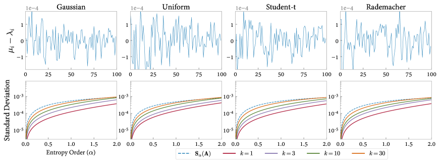
We first test the robustness of 𝐒αk(𝐀)superscriptsubscript𝐒𝛼𝑘𝐀{\bf S}_{\alpha}^{k}({\bf A}) against noises in the data. As indicated by Theorem 1, low-rank Rényi’s entropy achieves lower variance under mild conditions in terms of the information potential. We consider the case that the input data points are randomly perturbed, i.e. 𝐲i=𝐱i+ε𝐩isubscript𝐲𝑖subscript𝐱𝑖𝜀subscript𝐩𝑖{\bf y}_{i}={\bf x}_{i}+\varepsilon{\bf p}_{i} for i[1,n]𝑖1𝑛i\in[1,n], where 𝐩isubscript𝐩𝑖{\bf p}_{i} is comprised of i.i.d. random variables. Let {λi}i=1nsuperscriptsubscriptsubscript𝜆𝑖𝑖1𝑛\{\lambda_{i}\}_{i=1}^{n}, {μi}i=1nsuperscriptsubscriptsubscript𝜇𝑖𝑖1𝑛\{\mu_{i}\}_{i=1}^{n} denote the eigenvalues of normalized kernel matrices constructed from {𝐱i}i=1nsuperscriptsubscriptsubscript𝐱𝑖𝑖1𝑛\{{\bf x}_{i}\}_{i=1}^{n} and {𝐲i}i=1nsuperscriptsubscriptsubscript𝐲𝑖𝑖1𝑛\{{\bf y}_{i}\}_{i=1}^{n} respectively. We test the following noise distributions: Standard Gaussian N(0,1)𝑁01N(0,1), Uniform U(3,3)𝑈33U(-\sqrt{3},\sqrt{3}), Student-t t(3)/3𝑡33t(3)/\sqrt{3} and Rademacher {±1}plus-or-minus1\{\pm 1\} with n=100𝑛100n=100 (detailed settings are given in the appendix). The examples of variation in eigenvalues (μiλisubscript𝜇𝑖subscript𝜆𝑖\mu_{i}-\lambda_{i}) and the standard deviation (multiplied by n𝑛n) of entropy values after 100100100 trials are reported in Figure 3. It verifies our analysis that when ε𝜀\varepsilon is small, the eigenvalues μisubscript𝜇𝑖\mu_{i} are nearly independently perturbed. Moreover, our low-rank definition achieves lower variance than matrix-based Rényi’s entropy under different choices of α𝛼\alpha, in which smaller k𝑘k corresponds to higher robustness.

Refer to caption
Figure 3: Upper: perturbation of the eigenvalues, i.e. μiλisubscript𝜇𝑖subscript𝜆𝑖\mu_{i}-\lambda_{i}. Lower: standard deviation of matrix-based Rényi’s entropy and low-rank Rényi’s entropy against random perturbations of the data samples for different values of α𝛼\alpha.

Real Data Examples

In this section, we demonstrate the great potential of applying our low-rank Rényi’s entropy functional and its multivariate extensions in two representative real-world information-related applications, which utilize the mutual information (information bottleneck) and multivariate mutual information (feature selection) respectively.

Objective Accuracy (%) Training Time (minutes)
CE 92.64 ±plus-or-minus\pm 0.03 0- / 080
VIB 94.08 ±plus-or-minus\pm 0.02 04 / 084
NIB 94.01 ±plus-or-minus\pm 0.04 07 / 087
MRIB 94.13 ±plus-or-minus\pm 0.04 46 / 126
LRIB 94.16 ±plus-or-minus\pm 0.09 15 / 095
Table 1: Classification accuracy and training time of different IB objectives. Left is the time spent on IB calculation and right is the total training time.
Method Criterion Breast Semeion Madelon Krvskp Spambase Waveform Optdigits Statlog Average
MIFS 𝐈(𝐗il;𝐘)βj=1l1𝐈(𝐗il;𝐗ij)𝐈subscript𝐗subscript𝑖𝑙𝐘𝛽superscriptsubscript𝑗1𝑙1𝐈subscript𝐗subscript𝑖𝑙subscript𝐗subscript𝑖𝑗\scriptstyle{\bf I}({\bf X}_{i_{l}};{\bf Y})-\beta\sum_{j=1}^{l-1}{\bf I}({\bf X}_{i_{l}};{\bf X}_{i_{j}}) 4.8 2.5 6.6 3.8 7.3 6.4 4.5 3.8 4.96
FOU 𝐈(𝐗il;𝐘)j=1l1[𝐈(𝐗il;𝐗ij)𝐈(𝐗il;𝐗ij|𝐘)]𝐈subscript𝐗subscript𝑖𝑙𝐘superscriptsubscript𝑗1𝑙1delimited-[]𝐈subscript𝐗subscript𝑖𝑙subscript𝐗subscript𝑖𝑗𝐈subscript𝐗subscript𝑖𝑙conditionalsubscript𝐗subscript𝑖𝑗𝐘\scriptstyle{\bf I}({\bf X}_{i_{l}};{\bf Y})-\sum_{j=1}^{l-1}[{\bf I}({\bf X}_{i_{l}};{\bf X}_{i_{j}})-{\bf I}({\bf X}_{i_{l}};{\bf X}_{i_{j}}|{\bf Y})] 5.2 2.5 5.6 1.9 6.2 5.7 4.8 5.7 4.70
MRMR 𝐈(𝐗il;𝐘)1l1j=1l1𝐈(𝐗il;𝐗ij)𝐈subscript𝐗subscript𝑖𝑙𝐘1𝑙1superscriptsubscript𝑗1𝑙1𝐈subscript𝐗subscript𝑖𝑙subscript𝐗subscript𝑖𝑗\scriptstyle{\bf I}({\bf X}_{i_{l}};{\bf Y})-\frac{1}{l-1}\sum_{j=1}^{l-1}{\bf I}({\bf X}_{i_{l}};{\bf X}_{i_{j}}) 2.3 4.7 6.7 3.7 5.6 3.6 4.8 4.0 4.43
JMI j=1l1𝐈({𝐗il,𝐗ij};𝐘)superscriptsubscript𝑗1𝑙1𝐈subscript𝐗subscript𝑖𝑙subscript𝐗subscript𝑖𝑗𝐘\scriptstyle\sum_{j=1}^{l-1}{\bf I}(\{{\bf X}_{i_{l}},{\bf X}_{i_{j}}\};{\bf Y}) 5.1 5.2 3.0 3.7 4.2 2.3 3.8 3.5 3.85
CMIM minj=1l1𝐈(𝐗il;𝐘|𝐗ij)superscriptsubscript𝑗1𝑙1𝐈subscript𝐗subscript𝑖𝑙conditional𝐘subscript𝐗subscript𝑖𝑗\scriptstyle\min_{j=1}^{l-1}{\bf I}({\bf X}_{i_{l}};{\bf Y}|{\bf X}_{i_{j}}) 3.0 2.7 4.5 3.6 3.2 4.7 2.6 5.6 3.74
DISR j=1l1𝐈({𝐗il,𝐗ij};𝐘)/𝐇(𝐗il,𝐗ij,𝐘)superscriptsubscript𝑗1𝑙1𝐈subscript𝐗subscript𝑖𝑙subscript𝐗subscript𝑖𝑗𝐘𝐇subscript𝐗subscript𝑖𝑙subscript𝐗subscript𝑖𝑗𝐘\scriptstyle\sum_{j=1}^{l-1}{\bf I}(\{{\bf X}_{i_{l}},{\bf X}_{i_{j}}\};{\bf Y})/{\bf H}({\bf X}_{i_{l}},{\bf X}_{i_{j}},{\bf Y}) 7.3 5.7 4.0 3.2 3.9 2.3 6.9 5.8 4.89
MRMI 𝐈α({𝐗i1,𝐗i2,,𝐗il};𝐘)subscript𝐈𝛼subscript𝐗subscript𝑖1subscript𝐗subscript𝑖2subscript𝐗subscript𝑖𝑙𝐘\scriptstyle{\bf I}_{\alpha}(\{{\bf X}_{i_{1}},{\bf X}_{i_{2}},\cdots,{\bf X}_{i_{l}}\};{\bf Y}) 2.6 1.8 1.2 1.7 1.5 1.8 1.3 2.0 1.74
LRMI 𝐈αk({𝐗i1,𝐗i2,,𝐗il};𝐘)superscriptsubscript𝐈𝛼𝑘subscript𝐗subscript𝑖1subscript𝐗subscript𝑖2subscript𝐗subscript𝑖𝑙𝐘\scriptstyle{\bf I}_{\alpha}^{k}(\{{\bf X}_{i_{1}},{\bf X}_{i_{2}},\cdots,{\bf X}_{i_{l}}\};{\bf Y}) 2.6 1.4 1.1 1.6 1.5 1.5 1.3 2.1 1.64
Table 2: Information theoretic feature selection methods and their average rank over different number of features in each dataset. The first and second best performances are marked as bold and underlined respectively.

Application to Information Bottleneck

The Information Bottleneck (IB) methods recently achieve great success in compressing redundant or irrelevant information in the inputs and preventing overfitting in deep neural networks. Formally, given network input 𝐗𝐗{\bf X} and target label 𝐘𝐘{\bf Y}, the IB approach tries to extract a compressed intermediate representation 𝐙𝐙{\bf Z} from 𝐗𝐗{\bf X} that maintains minimal yet meaningful information to predict the task 𝐘𝐘{\bf Y} by optimizing the following IB Lagrangian:

IB=𝐈(𝐘,𝐙)β𝐈(𝐗,𝐙),subscriptIB𝐈𝐘𝐙𝛽𝐈𝐗𝐙\mathcal{L}_{\textrm{IB}}={\bf I}({\bf Y},{\bf Z})-\beta\cdot{\bf I}({\bf X},{\bf Z}),

where β𝛽\beta is the hyper-parameter that balances the trade-off between sufficiency (predictive performance of 𝐙𝐙{\bf Z} on task 𝐘𝐘{\bf Y}, quantified by 𝐈(𝐘,𝐙)𝐈𝐘𝐙{\bf I}({\bf Y},{\bf Z})) and minimality (the complexity of 𝐙𝐙{\bf Z}, quantified by 𝐈(𝐗,𝐙)𝐈𝐗𝐙{\bf I}({\bf X},{\bf Z})). In practice, optimizing 𝐈(𝐘,𝐙)𝐈𝐘𝐙{\bf I}({\bf Y},{\bf Z}) is equivalent to the cross-entropy (CE) loss for classification tasks, so our target remains to optimize the latter term 𝐈(𝐗,𝐙)𝐈𝐗𝐙{\bf I}({\bf X},{\bf Z}). However, mutual information estimation is extremely hard or even intractable for high-dimension distributions, which is usually the case in deep learning. To address this issue, there have been efforts on using variational approximations to optimize a lower bound of 𝐈(𝐗,𝐙)𝐈𝐗𝐙{\bf I}({\bf X},{\bf Z}), e.g. Variational IB (VIB) (Alemi et al. 2017) and Nonlinear IB (NIB) (Kolchinsky, Tracey, and Wolpert 2019). We show that with low-rank Rényi’s entropy, 𝐈(𝐗,𝐙)𝐈𝐗𝐙{\bf I}({\bf X},{\bf Z}) can be directly optimized by approximating the largest k𝑘k eigenvalues of the kernel matrix 𝐀𝐀{\bf A} constructed by 𝐗𝐗{\bf X} and 𝐙𝐙{\bf Z}. Recall that the Lanczos method constructs an approximation 𝐀𝐐𝐓𝐐𝐀superscript𝐐𝐓𝐐top{\bf A}\approx{\bf Q}{\bf T}{\bf Q}^{\top}, where 𝐐n×s𝐐superscript𝑛𝑠{\bf Q}\in\mathbb{R}^{n\times s} has orthogonal columns and 𝐓s×s𝐓superscript𝑠𝑠{\bf T}\in\mathbb{R}^{s\times s} is tridiagonal, we have λ^i=λi(𝐐𝐀𝐐)subscript^𝜆𝑖subscript𝜆𝑖superscript𝐐top𝐀𝐐\hat{\lambda}_{i}=\lambda_{i}({\bf Q}^{\top}{\bf A}{\bf Q}) for all i[1,s]𝑖1𝑠i\in[1,s]. Let i=1sλ^i𝐮i𝐮isuperscriptsubscript𝑖1𝑠subscript^𝜆𝑖subscript𝐮𝑖superscriptsubscript𝐮𝑖top\sum_{i=1}^{s}\hat{\lambda}_{i}{\bf u}_{i}{\bf u}_{i}^{\top} be the eigenvalue decomposition of 𝐐𝐀𝐐superscript𝐐top𝐀𝐐{\bf Q}^{\top}{\bf A}{\bf Q}, we can approximate the gradient of 𝐒αk(𝐀)superscriptsubscript𝐒𝛼𝑘𝐀{\bf S}_{\alpha}^{k}({\bf A}) as:

𝐒αk(𝐀)𝐀i=1k𝐒^αk(𝐀)λ^i𝐐𝐮i𝐮i𝐐.superscriptsubscript𝐒𝛼𝑘𝐀𝐀superscriptsubscript𝑖1𝑘superscriptsubscript^𝐒𝛼𝑘𝐀subscript^𝜆𝑖subscript𝐐𝐮𝑖superscriptsubscript𝐮𝑖topsuperscript𝐐top\frac{\partial{\bf S}_{\alpha}^{k}({\bf A})}{\partial{\bf A}}\approx\sum_{i=1}^{k}\frac{\partial\hat{{\bf S}}_{\alpha}^{k}({\bf A})}{\partial\hat{\lambda}_{i}}\cdot{\bf Q}{\bf u}_{i}{\bf u}_{i}^{\top}{\bf Q}^{\top}.

In this experiment, we test the performance of matrix-based Rényi’s IB (MRIB) (Yu, Yu, and Principe 2021) and our low-rank variant (LRIB) with variational approximation-based objectives using VGG16 as the backbone and CIFAR10 as the classification task. All models are trained for 300300300 epochs with 100100100 batch size and 0.10.10.1 initial learning rate which is divided by 101010 every 100100100 epochs. Following the settings in (Yu, Yu, and Principe 2021), we select α=1.01𝛼1.01\alpha=1.01, β=0.01𝛽0.01\beta=0.01, k=10𝑘10k=10 and s=20𝑠20s=20. The final results are reported in Table 1. It can be seen that the matrix-based approaches MRIB and LRIB outperform other methods, while our LRIB achieves the highest performance with significantly less training time.

Application to Feature Selection

In practical regression or classification machine learning tasks, many features can be completely irrelevant to the learning target or redundant in the context of others. Given a set of features 𝐒={𝐗1,,𝐗L}𝐒subscript𝐗1subscript𝐗𝐿{\bf S}=\{{\bf X}_{1},\cdots,{\bf X}_{L}\} and the target label 𝐘𝐘{\bf Y}, we aim to find a subset 𝐒sub𝐒subscript𝐒𝑠𝑢𝑏𝐒{\bf S}_{sub}\subset{\bf S} which leverage the expressiveness and the complexity simultaneously. In the field of information theoretic learning, this target is equivalent to maximizing the multivariate mutual information 𝐈(𝐒sub;𝐘)𝐈subscript𝐒𝑠𝑢𝑏𝐘{\bf I}({\bf S}_{sub};{\bf Y}), which is computationally prohibitive due to the curse of high dimensionality. As a result, there have been tremendous efforts on approximation techniques that retain only the first or second order interactions and build mutual information estimators upon low-dimensional probability distributions, including Mutual Information-based Feature Selection (MIFS) (R. Battiti 1994), First-Order Utility (FOU) (Brown 2009), Maximum-Relevance Minimum-Redundancy (MRMR) (Peng, Long, and Ding 2005), Joint Mutual Information (JMI) (Yang and Moody 1999), Conditional Mutual Information Maximization (CMIM) (Fleuret 2004) and Double Input Symmetrical Relevance (DISR) (Meyer and Bontempi 2006) which achieve state-of-the-art performance in information-based feature selection tasks.

We evaluate the performance of matrix-based Rényi’s mutual information (MRMI) and our low-rank variant (LRMI) with these methods on 888 widely-used classification datasets as shown in Table 3, which is chosen to cover a broad variety of instance-feature ratios, number of classes and discreteness. Notice that non-Rényi methods can only handle discrete features, so we discretize them into 555 bins under equal-width criterion as adopted in (Brown et al. 2012). In this experiment, we choose the Support Vector Machine (SVM) algorithm with RBF kernel (σ=1𝜎1\sigma=1) as the classifier for continuous datasets and a 3-NN classifier for discrete datasets. Following the settings of (Yu et al. 2019), we select α{0.6,1.01,2}𝛼0.61.012\alpha\in\{0.6,1.01,2\}, k{100,200,400}𝑘100200400k\in\{100,200,400\} via cross-validation, s=k+50𝑠𝑘50s=k+50 and use the Gaussian kernel of width σ=1𝜎1\sigma=1 for matrix-based entropy measures. Considering that it is NP-hard to evaluate each subset of 𝐒𝐒{\bf S}, we adopt a greedy strategy to incrementally select 101010 features that maximize our target 𝐈(𝐒sub;𝐘)𝐈subscript𝐒𝑠𝑢𝑏𝐘{\bf I}({\bf S}_{sub};{\bf Y}). That is, in each step, we fix the current subset 𝐒sub={𝐗i1,,𝐗il1}subscript𝐒𝑠𝑢𝑏subscript𝐗subscript𝑖1subscript𝐗subscript𝑖𝑙1{\bf S}_{sub}=\{{\bf X}_{i_{1}},\cdots,{\bf X}_{i_{l-1}}\} and add a new feature 𝐗il𝐒/𝐒subsubscript𝐗subscript𝑖𝑙𝐒subscript𝐒𝑠𝑢𝑏{\bf X}_{i_{l}}\in{\bf S}/{\bf S}_{sub} to 𝐒subsubscript𝐒𝑠𝑢𝑏{\bf S}_{sub}. The average rank of each method across different number of features and the running time of MRMI and LRMI are reported in Table 2 and Table 3.

Dataset #I #F #C Discrete Time Speedup
Breast 569 30 2 No 0.31  / 0.25 1.2
Semeion 1593 256 10 Yes 56  / 44 1.3
Madelon 2600 500 2 Yes 570  / 39 14.4
Krvskp 3196 36 2 Yes 71  / 11 6.6
Spambase 4601 56 2 No 353  / 13 27.2
Waveform 5000 40 3 No 318  / 14 22.5
Optdigits 5620 64 10 Yes 750  / 41 18.4
Statlog 6435 36 6 Yes 600  / 23 25.7
Table 3: Number of instances (#I), features (#F), classes (#C) and discreteness of classification datasets used in feature selection experiments, running time comparison (minutes) of MRMI (left) and LRMI (right), and speedup ratios.

As we can see, both MRMI and LRMI significantly outperform other Shannon entropy based methods. Compared to MRMI, LRMI achieves 666 to 272727 times speedup, 151515 times on average via Lanczos approximation. Furthermore, LRMI outperforms MRMI on 444 datasets in our test benchmark, which verifies our theoretical analysis that low-rank Rényi’s entropy enables higher robustness against noises in the data. This demonstrates the great potential of our low-rank Rényi’s entropy on information-related tasks.

Conclusion

In this paper, we investigate an alternative entropy measure built upon the largest k𝑘k eigenvalues of the data kernel matrix. Compared to the original matrix-based Rényi’s entropy, our definition enables higher robustness to noises in the data and sensitivity to informative changes in eigenspectrum distribution with a proper choice of hyper-parameter k𝑘k. Moreover, low-rank Rényi’s entropy can be efficiently approximated with 𝒪(ns2)𝒪𝑛superscript𝑠2\mathcal{O}(ns^{2}) random projection and 𝒪(n2s)𝒪superscript𝑛2𝑠\mathcal{O}(n^{2}s) Lanczos iteration techniques, substantially lower than the 𝒪(n3)𝒪superscript𝑛3\mathcal{O}(n^{3}) complexity required to compute matrix-based Rényi’s entropy. We conduct large-scale simulation and real-world experiments on information bottleneck and feature selection tasks to validate the effectiveness of low-rank Rényi’s entropy, demonstrating elegant performance with significant improvements in computational efficiency.

Acknowledgments

This work was supported by National Key Research and Development Program of China (2021ZD0110700), National Natural Science Foundation of China (62106191, 12071166, 62192781, 61721002), the Research Council of Norway (RCN) under grant 309439, Innovation Research Team of Ministry of Education (IRT_17R86), Project of China Knowledge Centre for Engineering Science and Technology and Project of Chinese Academy of Engineering (The Online and Offline Mixed Educational Service System for The Belt and Road Training in MOOC China).

Supplementary Experimental Results

Parameter Settings of Robustness Experiment

In the first simulation study, we set n=100𝑛100n=100, d=400𝑑400d=400, ε=1/n=0.01𝜀1𝑛0.01\varepsilon=1/n=0.01 and use the linear kernel κ(𝐱i,𝐱j)=𝐱i𝐱j𝜅subscript𝐱𝑖subscript𝐱𝑗superscriptsubscript𝐱𝑖topsubscript𝐱𝑗\kappa({\bf x}_{i},{\bf x}_{j})={\bf x}_{i}^{\top}{\bf x}_{j} to generate the kernel matrices. The data samples {𝐱i}i=1nsuperscriptsubscriptsubscript𝐱𝑖𝑖1𝑛\{{\bf x}_{i}\}_{i=1}^{n} are generated by i.i.d Gaussian distribution N(0,0.12)𝑁0superscript0.12N(0,0.1^{2}). The noise distributions \mathcal{E} are selected following the criterion that 𝐄[]=0𝐄delimited-[]0{\bf E}[\mathcal{E}]=0 and 𝐕𝐚𝐫[]=1𝐕𝐚𝐫delimited-[]1{\bf Var}[\mathcal{E}]=1. It can be seen that we get similar results under different noise settings, which further verifies our analysis that when ε𝜀\varepsilon is small, the variance of 𝐒αk(𝐀)superscriptsubscript𝐒𝛼𝑘𝐀{\bf S}_{\alpha}^{k}({\bf A}) mainly depends on the variance of random perturbations of data samples.

Additional Results of Approximation Algorithms

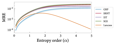
Additionally, we evaluate the impact of α𝛼\alpha and c𝑐c on approximation accuracy. We keep the previous n=8192𝑛8192n=8192 parameter settings and set k=64𝑘64k=64. The results of MRE curves with c=1.0𝑐1.0c=1.0 and varying α𝛼\alpha are reported in Figure 4. For SGS, we set the sparsity hyper-parameter p=2𝑝2p=2. For Lanczos, we randomly select the initial vector 𝐪𝐪{\bf q} from standard Gaussian. It can be seen that GRP achieves the lowest MRE amongst all random projection algorithms. When α𝛼\alpha is small, all MRE curves exhibit similar behavior and grow with the increase of α𝛼\alpha. This behavior starts to differ when α𝛼\alpha gets larger. For random projection algorithms, MRE keeps at the same level; for Lanczos algorithm, MRE starts to decrease when α>2𝛼2\alpha>2. Recall that the larger eigenvalues of 𝐀𝐀{\bf A} take the main role in the calculation of 𝐒αk(𝐀)superscriptsubscript𝐒𝛼𝑘𝐀{\bf S}_{\alpha}^{k}({\bf A}) for large α𝛼\alpha, this phenomenon indicates that Lanczos algorithm achieves higher precision for larger eigenvalues than smaller ones (as shown in our proof, it requires only 𝒪(i+log(1/ϵ))𝒪𝑖1italic-ϵ\mathcal{O}(i+\log(1/\epsilon)) steps to approximate λisubscript𝜆𝑖\lambda_{i} to relative error 1±ϵplus-or-minus1italic-ϵ1\pm\epsilon), while random projection achieves similar level of precision for all of the k𝑘k eigenvalues.

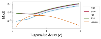
We then evaluate the impact of EDR (c) on approximation accuracy. In Figure 5, we report the MRE curves for α=2𝛼2\alpha=2 while c𝑐c varies from 00 (flat) to 222 (steep). It is interesting that the behavior of the two types of methods is entirely different. For random projections, the MRE curves grow slowly (GRP) or keep unchanged (SRHT, IST and SGS) when c𝑐c is small, and start to increase at a constant rate when c𝑐c gets large. This is because 𝐒αk(𝐀)superscriptsubscript𝐒𝛼𝑘𝐀{\bf S}_{\alpha}^{k}({\bf A}) is decreasing along with the increase of c𝑐c, whose slope is low at first and high when c𝑐c gets large (see Figure 2). This results in the slow to fast increasing behavior in relative error since the absolute error is upper bounded (Theorem 2). For Lanczos method, the ratio λ1/λrsubscript𝜆1subscript𝜆𝑟\lambda_{1}/\lambda_{r} in Theorem 3 increases fast when c𝑐c is small, resulting in the increase of MRE. When c𝑐c gets large, λ1subscript𝜆1\lambda_{1} gradually reaches its upper bound λ11subscript𝜆11\lambda_{1}\leq 1, while the intervals between adjacent eigenvalues also increase and result in a higher R𝑅R (Theorem 3). Moreover, recall that Lanczos algorithm approximates larger eigenvalues to higher precision, these reasons together explain the increase and then decrease MRE of the Lanczos approach.

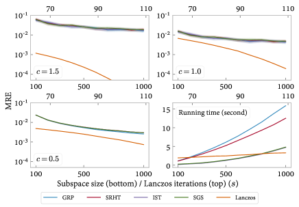
Next, we conduct large-scale experiments to evaluate the approximation algorithms. The kernel matrices are generated by 𝐀=𝚽𝚺𝚽𝐀𝚽𝚺superscript𝚽top{\bf A}=\bm{\Phi}\bm{\Sigma}\bm{\Phi}^{\top}, where 𝚽n×n𝚽superscript𝑛𝑛\bm{\Phi}\in\mathbb{R}^{n\times n} is a random orthogonal matrix, 𝚺n×n𝚺superscript𝑛𝑛\bm{\Sigma}\in\mathbb{R}^{n\times n} is a diagonal matrix such that 𝚺ii=icsubscript𝚺𝑖𝑖superscript𝑖𝑐\bm{\Sigma}_{ii}=i^{-c} for i[1,n]𝑖1𝑛i\in[1,n], and c𝑐c is a constant that controls the EDR. We set size of the kernel matrix n=8192𝑛8192n=8192. For random projection methods, we make s𝑠s vary from 100100100 to 100010001000; while for Lanczos algorithm, s𝑠s varies from 646464 to 110110110. The mean relative error (MRE) and ±14plus-or-minus14\pm\frac{1}{4} standard deviation (SD) are reported in Figure 6 for each test after 100100100 trials with α=1.5𝛼1.5\alpha=1.5 and c{1.5,1.0,0.5}𝑐1.51.00.5c\in\{1.5,1.0,0.5\}, which correspond to high, medium and low EDR respectively. For comparison, the trivial eigenvalue decomposition approach requires 134134134 seconds. It can be seen that all random projection methods yield similar approximation accuracy, in which GRP achieves slightly lower MRE when c=0.5𝑐0.5c=0.5 while IST & SGS bring the highest speedup. The Lanczos method achieves the highest accuracy with significantly lower s𝑠s values but requires longer running time. Generally, we recommend IST or SGS for medium precision approximation, and Lanczos when high precision is required. These methods achieve more than 252525 times speedup compared to the trivial approach for an 8192×8192819281928192\times 8192 kernel matrix.

Additional Results of Feature Selection

The hyper-parameter selection result of α𝛼\alpha and k𝑘k for matrix-based Rényi’s entropy and low-rank Rényi’s entropy in feature selection experiment via cross-validation are shown in Table 4. As can be seen, k=100𝑘100k=100 is already suitable for most circumstances. We perform a Nemenyi’s post-hoc test (Demvsar 2006) to give the significant level, in which the confidence that method i𝑖i significantly outperforms method j𝑗j is calculated as:

pij=𝚽((RjRi)/M(M+1)6N),p_{ij}=\bm{\Phi}\left\lparen\left.(R_{j}-R_{i})\middle/\sqrt{\frac{M(M+1)}{6N}}\right.\right\rparen,

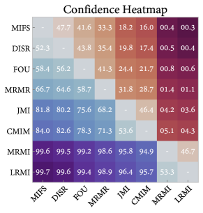
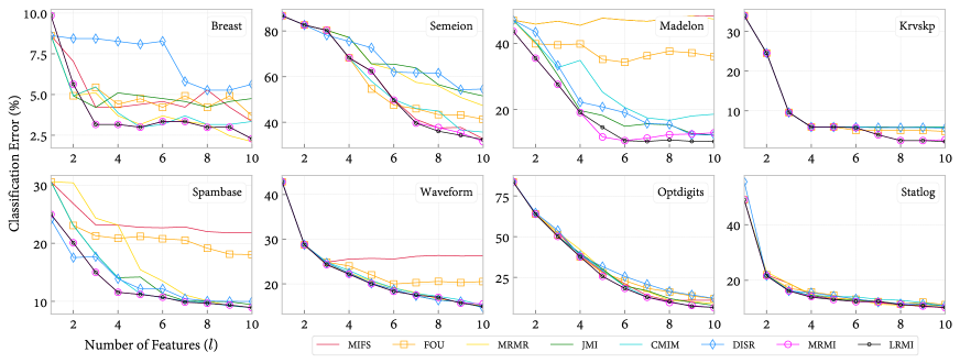
where 𝚽𝚽\bm{\Phi} is the CDF of standard normal distribution, Risubscript𝑅𝑖R_{i} is the average rank of method i𝑖i, M𝑀M is the number of methods and N𝑁N is the number of datasets. For our case, we have M=8𝑀8M=8, N=8𝑁8N=8 and the value of Risubscript𝑅𝑖R_{i} are given in the last column of table 2. The confidence level of different methods is shown in Figure 7. It can be seen that under significance level p=0.05𝑝0.05p=0.05, LRMI significantly outperforms all Shannon’s entropy-based methods, while the confidence of MRMI outperforming CMIM is not significant enough. In Figure 8, we report the classification accuracy achieved by different feature selection methods for the first 101010 features. It can be seen that classification error tends to stabilize after selecting the 101010 most informative features.

Refer to caption
Figure 4: α𝛼\alpha versus MRE curves for entropy approximation.
Refer to caption
Figure 5: c𝑐c versus MRE curves for entropy approximation.
Refer to caption
Figure 6: s𝑠s versus MRE curves for entropy approximation. The first three sub-figure correspond to different c𝑐c values, while the last sub-figure show the running time.
Dataset α𝛼\alpha k𝑘k
Breast 2.0 100
Semeion 1.01 400
Madelon 2.0 100
Krvskp 1.01 200
Spambase 2.0 100
Waveform 2.0 100
Optdigits 1.01 200
Statlog 0.6 100
Table 4: Hyper-parameter selection results of α𝛼\alpha and k𝑘k in feature selection experiment.
Refer to caption
Figure 7: Confidence of significant outperforming (%) for different feature selection methods.
Refer to caption
Figure 8: Number of Features (l𝑙l) versus Classification Error (%) curves for different feature selection methods.

Proof of Main Results

Proof of Proposition 1

Proof.

For (a): Let 𝐀=𝐔𝚲𝐔𝐀𝐔𝚲superscript𝐔top{\bf A}={\bf U}\bm{\Lambda}{\bf U}^{\top} be the eigenvalue decomposition of 𝐀𝐀{\bf A}, then 𝐏𝐔𝐏𝐔{\bf P}{\bf U} is a unitary matrix and λi(𝐀)=λi(𝐏𝐀𝐏)subscript𝜆𝑖𝐀subscript𝜆𝑖superscript𝐏𝐀𝐏top\lambda_{i}({\bf A})=\lambda_{i}({\bf P}{\bf A}{\bf P}^{\top}) for all i[1,k]𝑖1𝑘i\in[1,k].

For (b): When p>0𝑝0p>0, 𝐭𝐫((pLk(𝐀))α)=pα𝐭𝐫(Lkα(𝐀))>0𝐭𝐫superscript𝑝subscript𝐿𝑘𝐀𝛼superscript𝑝𝛼𝐭𝐫superscriptsubscript𝐿𝑘𝛼𝐀0{\bf tr}\left\lparen(pL_{k}({\bf A}))^{\alpha}\right\rparen=p^{\alpha}\cdot{\bf tr}(L_{k}^{\alpha}({\bf A}))>0, then (b) follows by the continuity of the logarithm function.

For (c): Notice that 𝐒αk(𝐀)=𝐒α(Lk(𝐀))superscriptsubscript𝐒𝛼𝑘𝐀subscript𝐒𝛼subscript𝐿𝑘𝐀{\bf S}_{\alpha}^{k}({\bf A})={\bf S}_{\alpha}(L_{k}({\bf A})), where 𝐭𝐫(Lk(𝐀))=1𝐭𝐫subscript𝐿𝑘𝐀1{\bf tr}(L_{k}({\bf A}))=1 and λi(Lk(𝐀))[0,1]subscript𝜆𝑖subscript𝐿𝑘𝐀01\lambda_{i}(L_{k}({\bf A}))\in[0,1] for all i[1,n]𝑖1𝑛i\in[1,n]. Then we have 𝐭𝐫(Lkα(𝐀))1𝐭𝐫superscriptsubscript𝐿𝑘𝛼𝐀1{\bf tr}(L_{k}^{\alpha}({\bf A}))\geq 1 when α(0,1)𝛼01\alpha\in(0,1) and 𝐭𝐫(Lkα(𝐀))1𝐭𝐫superscriptsubscript𝐿𝑘𝛼𝐀1{\bf tr}(L_{k}^{\alpha}({\bf A}))\leq 1 when α>1𝛼1\alpha>1, which further implies that 𝐒αk(𝐀)0superscriptsubscript𝐒𝛼𝑘𝐀0{\bf S}_{\alpha}^{k}({\bf A})\geq 0.

Let f(x)=xα𝑓𝑥superscript𝑥𝛼f(x)=x^{\alpha}, it is obvious that f𝑓f is concave when α(0,1)𝛼01\alpha\in(0,1) and convex when α>1𝛼1\alpha>1. Then by Jensen’s inequality, 𝐭𝐫(f(Lk(𝐀)))𝐭𝐫(f(1nI))𝐭𝐫𝑓subscript𝐿𝑘𝐀𝐭𝐫𝑓1𝑛𝐼{\bf tr}(f(L_{k}({\bf A})))\leq{\bf tr}(f(\frac{1}{n}I)) when α(0,1)𝛼01\alpha\in(0,1) and otherwise the opposite, which further implies that 𝐒αk(𝐀)𝐒αk(1nI)superscriptsubscript𝐒𝛼𝑘𝐀superscriptsubscript𝐒𝛼𝑘1𝑛𝐼{\bf S}_{\alpha}^{k}({\bf A})\leq{\bf S}_{\alpha}^{k}(\frac{1}{n}I).

Moreover, it is straightforward to show that 𝐒αk(1nI)=𝐒α(1nI)=log2(n)superscriptsubscript𝐒𝛼𝑘1𝑛𝐼subscript𝐒𝛼1𝑛𝐼subscript2𝑛{\bf S}_{\alpha}^{k}(\frac{1}{n}I)={\bf S}_{\alpha}(\frac{1}{n}I)=\log_{2}(n).

For (d): From Proposition 4.1 in (Sanchez Giraldo, Rao, and Principe 2014) we have that 𝐒α(𝐀𝐁)=𝐒α(𝐀)+𝐒α(𝐁)subscript𝐒𝛼tensor-product𝐀𝐁subscript𝐒𝛼𝐀subscript𝐒𝛼𝐁{\bf S}_{\alpha}({\bf A}\otimes{\bf B})={\bf S}_{\alpha}({\bf A})+{\bf S}_{\alpha}({\bf B}), therefore 𝐒α(Lk(𝐀)Lk(𝐁))=𝐒α(Lk(𝐀))+𝐒α(Lk(𝐁))subscript𝐒𝛼tensor-productsubscript𝐿𝑘𝐀subscript𝐿𝑘𝐁subscript𝐒𝛼subscript𝐿𝑘𝐀subscript𝐒𝛼subscript𝐿𝑘𝐁{\bf S}_{\alpha}(L_{k}({\bf A})\otimes L_{k}({\bf B}))={\bf S}_{\alpha}(L_{k}({\bf A}))+{\bf S}_{\alpha}(L_{k}({\bf B})). Notice that the smaller (nk)2superscript𝑛𝑘2(n-k)^{2} eigenvalues of Lk(𝐀)Lk(𝐁)tensor-productsubscript𝐿𝑘𝐀subscript𝐿𝑘𝐁L_{k}({\bf A})\otimes L_{k}({\bf B}) are equal to λr(𝐀)λr(𝐁)subscript𝜆𝑟𝐀subscript𝜆𝑟𝐁\lambda_{r}({\bf A})\lambda_{r}({\bf B}), we have 𝐒αn2(nk)2(Lk(𝐀)Lk(𝐁))=𝐒αk(Lk(𝐀))+𝐒αk(Lk(𝐁))superscriptsubscript𝐒𝛼superscript𝑛2superscript𝑛𝑘2tensor-productsubscript𝐿𝑘𝐀subscript𝐿𝑘𝐁superscriptsubscript𝐒𝛼𝑘subscript𝐿𝑘𝐀superscriptsubscript𝐒𝛼𝑘subscript𝐿𝑘𝐁{\bf S}_{\alpha}^{n^{2}-(n-k)^{2}}(L_{k}({\bf A})\otimes L_{k}({\bf B}))={\bf S}_{\alpha}^{k}(L_{k}({\bf A}))+{\bf S}_{\alpha}^{k}(L_{k}({\bf B})).

For (e): From Proposition 4.1 in (Sanchez Giraldo, Rao, and Principe 2014) we have that 𝐒α(t𝐀k+(1t)𝐁k)=g1(tg(𝐒α(𝐀))+(1t)g(𝐒α(𝐁)))subscript𝐒𝛼𝑡subscript𝐀𝑘1𝑡subscript𝐁𝑘superscript𝑔1𝑡𝑔subscript𝐒𝛼𝐀1𝑡𝑔subscript𝐒𝛼𝐁{\bf S}_{\alpha}(t{\bf A}_{k}+(1-t){\bf B}_{k})=g^{-1}\big{(}tg({\bf S}_{\alpha}({\bf A}))+(1-t)g({\bf S}_{\alpha}({\bf B}))\big{)}. Notice that 𝐀k=𝐀subscript𝐀𝑘𝐀{\bf A}_{k}={\bf A} when 𝐭𝐫(𝐀k)=1𝐭𝐫subscript𝐀𝑘1{\bf tr}({\bf A}_{k})=1, we have 𝐒αk(t𝐀+(1t)𝐁)=g1(tg(𝐒αk(𝐀))+(1t)g(𝐒αk(𝐁)))superscriptsubscript𝐒𝛼𝑘𝑡𝐀1𝑡𝐁superscript𝑔1𝑡𝑔superscriptsubscript𝐒𝛼𝑘𝐀1𝑡𝑔superscriptsubscript𝐒𝛼𝑘𝐁{\bf S}_{\alpha}^{k}(t{\bf A}+(1-t){\bf B})=g^{-1}\big{(}tg({\bf S}_{\alpha}^{k}({\bf A}))+(1-t)g({\bf S}_{\alpha}^{k}({\bf B}))\big{)}.

For (f): From the proof of Proposition 4.1 in (Sanchez Giraldo, Rao, and Principe 2014) we have that

i=1tλi(𝐀𝐁)1ni=1tλi(𝐁),superscriptsubscript𝑖1𝑡subscript𝜆𝑖𝐀𝐁1𝑛superscriptsubscript𝑖1𝑡subscript𝜆𝑖𝐁\sum_{i=1}^{t}\lambda_{i}({\bf A}\circ{\bf B})\leq\frac{1}{n}\sum_{i=1}^{t}\lambda_{i}({\bf B}),

where t𝑡t is any integer in [1,n]1𝑛[1,n]. Therefore

i=1tλi(Lk(𝐀𝐁))superscriptsubscript𝑖1𝑡subscript𝜆𝑖subscript𝐿𝑘𝐀𝐁\displaystyle\sum_{i=1}^{t}\lambda_{i}(L_{k}({\bf A}\circ{\bf B})) 1ni=1tλi(Lk(𝐁)),t[1,k],formulae-sequenceabsent1𝑛superscriptsubscript𝑖1𝑡subscript𝜆𝑖subscript𝐿𝑘𝐁for-all𝑡1𝑘\displaystyle\leq\frac{1}{n}\sum_{i=1}^{t}\lambda_{i}(L_{k}({\bf B})),\quad\forall t\in[1,k],
i=1nλi(Lk(𝐀𝐁))superscriptsubscript𝑖1𝑛subscript𝜆𝑖subscript𝐿𝑘𝐀𝐁\displaystyle\sum_{i=1}^{n}\lambda_{i}(L_{k}({\bf A}\circ{\bf B})) =1ni=1nλi(Lk(𝐁))=1n,absent1𝑛superscriptsubscript𝑖1𝑛subscript𝜆𝑖subscript𝐿𝑘𝐁1𝑛\displaystyle=\frac{1}{n}\sum_{i=1}^{n}\lambda_{i}(L_{k}({\bf B}))=\frac{1}{n},

From the case t=k𝑡𝑘t=k we know that λr(𝐀𝐁)λr(𝐁)/nsubscript𝜆𝑟𝐀𝐁subscript𝜆𝑟𝐁𝑛\lambda_{r}({\bf A}\circ{\bf B})\geq\lambda_{r}({\bf B})/n, therefore for any t[k+1,n]𝑡𝑘1𝑛t\in[k+1,n], we have

i=1tλi(Lk(𝐀𝐁))superscriptsubscript𝑖1𝑡subscript𝜆𝑖subscript𝐿𝑘𝐀𝐁\displaystyle\sum_{i=1}^{t}\lambda_{i}(L_{k}({\bf A}\circ{\bf B})) =1n(nt)λr(𝐀𝐁)absent1𝑛𝑛𝑡subscript𝜆𝑟𝐀𝐁\displaystyle=\frac{1}{n}-(n-t)\lambda_{r}({\bf A}\circ{\bf B})
1nntnλr(𝐁)absent1𝑛𝑛𝑡𝑛subscript𝜆𝑟𝐁\displaystyle\leq\frac{1}{n}-\frac{n-t}{n}\lambda_{r}({\bf B})
=1ni=1tλi(Lk(𝐁)).absent1𝑛superscriptsubscript𝑖1𝑡subscript𝜆𝑖subscript𝐿𝑘𝐁\displaystyle=\frac{1}{n}\sum_{i=1}^{t}\lambda_{i}(L_{k}({\bf B})).

Then we can prove that

𝐒αk(𝐀𝐁𝐭𝐫(𝐀𝐁))superscriptsubscript𝐒𝛼𝑘𝐀𝐁𝐭𝐫𝐀𝐁\displaystyle{\bf S}_{\alpha}^{k}\left\lparen\frac{{\bf A}\circ{\bf B}}{{\bf tr}({\bf A}\circ{\bf B})}\right\rparen =𝐒α(Lk(𝐀𝐁𝐭𝐫(𝐀𝐁)))absentsubscript𝐒𝛼subscript𝐿𝑘𝐀𝐁𝐭𝐫𝐀𝐁\displaystyle={\bf S}_{\alpha}\left\lparen L_{k}\left\lparen\frac{{\bf A}\circ{\bf B}}{{\bf tr}({\bf A}\circ{\bf B})}\right\rparen\right\rparen
𝐒α(Lk(𝐁))=𝐒αk(𝐁)absentsubscript𝐒𝛼subscript𝐿𝑘𝐁superscriptsubscript𝐒𝛼𝑘𝐁\displaystyle\geq{\bf S}_{\alpha}(L_{k}({\bf B}))={\bf S}_{\alpha}^{k}({\bf B})

following the proof in (Sanchez Giraldo, Rao, and Principe 2014).

For (g): From the proof of Proposition 4.1 in (Sanchez Giraldo, Rao, and Principe 2014), when 𝐀=1n𝟏𝟏𝐀1𝑛superscript11top{\bf A}=\frac{1}{n}\mathbf{1}\mathbf{1}^{\top} and 𝐀=1nI𝐀1𝑛𝐼{\bf A}=\frac{1}{n}I, we have

i=1tλi(𝐀𝐁)superscriptsubscript𝑖1𝑡subscript𝜆𝑖𝐀𝐁\displaystyle\sum_{i=1}^{t}\lambda_{i}({\bf A}\circ{\bf B}) 1ni=1tλi(𝐁)andabsent1𝑛superscriptsubscript𝑖1𝑡subscript𝜆𝑖𝐁and\displaystyle\leq\frac{1}{n}\sum_{i=1}^{t}\lambda_{i}({\bf B})\quad\mathrm{and}
1ni=1tλi(𝐀𝐁)1𝑛superscriptsubscript𝑖1𝑡subscript𝜆𝑖𝐀𝐁\displaystyle\frac{1}{n}\sum_{i=1}^{t}\lambda_{i}({\bf A}\circ{\bf B}) 1ni=1tλi(𝐁)absent1𝑛superscriptsubscript𝑖1𝑡subscript𝜆𝑖𝐁\displaystyle\leq\frac{1}{n}\sum_{i=1}^{t}\lambda_{i}({\bf B})

respectively, where t𝑡t is any integer in [1,n]1𝑛[1,n]. Similar with the proof of (f), for these two extreme cases we can prove that

i=1tλi(Lk(𝐀𝐁))superscriptsubscript𝑖1𝑡subscript𝜆𝑖subscript𝐿𝑘𝐀𝐁\displaystyle\sum_{i=1}^{t}\lambda_{i}(L_{k}({\bf A}\circ{\bf B})) 1ni=1tλi(Lk(𝐁))andabsent1𝑛superscriptsubscript𝑖1𝑡subscript𝜆𝑖subscript𝐿𝑘𝐁and\displaystyle\leq\frac{1}{n}\sum_{i=1}^{t}\lambda_{i}(L_{k}({\bf B}))\quad\mathrm{and}
1ni=1tλi(Lk(𝐀𝐁))1𝑛superscriptsubscript𝑖1𝑡subscript𝜆𝑖subscript𝐿𝑘𝐀𝐁\displaystyle\frac{1}{n}\sum_{i=1}^{t}\lambda_{i}(L_{k}({\bf A}\circ{\bf B})) 1ni=1tλi(Lk(𝐁))absent1𝑛superscriptsubscript𝑖1𝑡subscript𝜆𝑖subscript𝐿𝑘𝐁\displaystyle\leq\frac{1}{n}\sum_{i=1}^{t}\lambda_{i}(L_{k}({\bf B}))

respectively. These inequalities imply that

𝐒α(Lk(𝐀𝐁𝐭𝐫(𝐀𝐁)))𝐒α(Lk(𝐀))+𝐒α(Lk(𝐁))subscript𝐒𝛼subscript𝐿𝑘𝐀𝐁𝐭𝐫𝐀𝐁subscript𝐒𝛼subscript𝐿𝑘𝐀subscript𝐒𝛼subscript𝐿𝑘𝐁{\bf S}_{\alpha}\left\lparen L_{k}\left\lparen\frac{{\bf A}\circ{\bf B}}{{\bf tr}({\bf A}\circ{\bf B})}\right\rparen\right\rparen\leq{\bf S}_{\alpha}(L_{k}({\bf A}))+{\bf S}_{\alpha}(L_{k}({\bf B}))

following the proof in (Sanchez Giraldo, Rao, and Principe 2014). ∎

Proof of Theorem 1

Proof.

Without loss of generality, we assume μ1μ2μnsubscript𝜇1subscript𝜇2subscript𝜇𝑛\mu_{1}\geq\mu_{2}\geq\cdots\geq\mu_{n}. Note that λisubscript𝜆𝑖\lambda_{i}, i[1,n]𝑖1𝑛i\in[1,n] may not be monotonically decreasing. By the definition of information potential, we have

𝐈𝐏α(𝐁)=i=1nμiα,subscript𝐈𝐏𝛼𝐁superscriptsubscript𝑖1𝑛superscriptsubscript𝜇𝑖𝛼\displaystyle{\bf IP}_{\alpha}({\bf B})=\sum_{i=1}^{n}\mu_{i}^{\alpha},
𝐈𝐏αk(𝐁)=i=1kμiα+(nk)μrα,superscriptsubscript𝐈𝐏𝛼𝑘𝐁superscriptsubscript𝑖1𝑘superscriptsubscript𝜇𝑖𝛼𝑛𝑘superscriptsubscript𝜇𝑟𝛼\displaystyle{\bf IP}_{\alpha}^{k}({\bf B})=\sum_{i=1}^{k}\mu_{i}^{\alpha}+(n-k)\mu_{r}^{\alpha},
μr=1nk(1i=1kμi).subscript𝜇𝑟1𝑛𝑘1superscriptsubscript𝑖1𝑘subscript𝜇𝑖\displaystyle\mu_{r}=\frac{1}{n-k}\left\lparen 1-\sum_{i=1}^{k}\mu_{i}\right\rparen.

When νisubscript𝜈𝑖\nu_{i} is small, we have the following first-order approximation:

μiαsuperscriptsubscript𝜇𝑖𝛼\displaystyle\mu_{i}^{\alpha} =(λi+νi)αabsentsuperscriptsubscript𝜆𝑖subscript𝜈𝑖𝛼\displaystyle=(\lambda_{i}+\nu_{i})^{\alpha}
=λiα+αλiα1νi+α(α1)2λiα2νi2+absentsuperscriptsubscript𝜆𝑖𝛼𝛼superscriptsubscript𝜆𝑖𝛼1subscript𝜈𝑖𝛼𝛼12superscriptsubscript𝜆𝑖𝛼2superscriptsubscript𝜈𝑖2\displaystyle=\lambda_{i}^{\alpha}+\alpha\lambda_{i}^{\alpha-1}\nu_{i}+\frac{\alpha(\alpha-1)}{2}\lambda_{i}^{\alpha-2}\nu_{i}^{2}+\cdots
=λiα+αλiα1νi+o(νi).absentsuperscriptsubscript𝜆𝑖𝛼𝛼superscriptsubscript𝜆𝑖𝛼1subscript𝜈𝑖𝑜subscript𝜈𝑖\displaystyle=\lambda_{i}^{\alpha}+\alpha\lambda_{i}^{\alpha-1}\nu_{i}+o(\nu_{i}).

Therefore

𝐕𝐚𝐫[𝐈𝐏α(𝐁)]𝐕𝐚𝐫delimited-[]subscript𝐈𝐏𝛼𝐁\displaystyle{\bf Var}[{\bf IP}_{\alpha}({\bf B})] =𝐕𝐚𝐫[𝐈𝐏α(𝐁)𝐈𝐏α(𝐀)]absent𝐕𝐚𝐫delimited-[]subscript𝐈𝐏𝛼𝐁subscript𝐈𝐏𝛼𝐀\displaystyle={\bf Var}[{\bf IP}_{\alpha}({\bf B})-{\bf IP}_{\alpha}({\bf A})]
=𝐕𝐚𝐫[i=1nμiαλiα]absent𝐕𝐚𝐫delimited-[]superscriptsubscript𝑖1𝑛superscriptsubscript𝜇𝑖𝛼superscriptsubscript𝜆𝑖𝛼\displaystyle={\bf Var}\left[\sum_{i=1}^{n}\mu_{i}^{\alpha}-\lambda_{i}^{\alpha}\right]
=𝐕𝐚𝐫[i=1nαλiα1νi+o(νi)]absent𝐕𝐚𝐫delimited-[]superscriptsubscript𝑖1𝑛𝛼superscriptsubscript𝜆𝑖𝛼1subscript𝜈𝑖𝑜subscript𝜈𝑖\displaystyle={\bf Var}\left[\sum_{i=1}^{n}\alpha\lambda_{i}^{\alpha-1}\nu_{i}+o(\nu_{i})\right]
α2i=1n𝐕𝐚𝐫[λiα1νi]absentsuperscript𝛼2superscriptsubscript𝑖1𝑛𝐕𝐚𝐫delimited-[]superscriptsubscript𝜆𝑖𝛼1subscript𝜈𝑖\displaystyle\approx\alpha^{2}\sum_{i=1}^{n}{\bf Var}\left[\lambda_{i}^{\alpha-1}\nu_{i}\right]
=α2i=1nσi2λi2(α1).absentsuperscript𝛼2superscriptsubscript𝑖1𝑛superscriptsubscript𝜎𝑖2superscriptsubscript𝜆𝑖2𝛼1\displaystyle=\alpha^{2}\sum_{i=1}^{n}\sigma_{i}^{2}\lambda_{i}^{2(\alpha-1)}.

Similarly, we have

𝐕𝐚𝐫[𝐈𝐏αk(𝐁)]𝐕𝐚𝐫delimited-[]superscriptsubscript𝐈𝐏𝛼𝑘𝐁\displaystyle{\bf Var}[{\bf IP}_{\alpha}^{k}({\bf B})] =𝐕𝐚𝐫[𝐈𝐏αk(𝐁)𝐈𝐏αk(𝐀)]absent𝐕𝐚𝐫delimited-[]superscriptsubscript𝐈𝐏𝛼𝑘𝐁superscriptsubscript𝐈𝐏𝛼𝑘𝐀\displaystyle={\bf Var}[{\bf IP}_{\alpha}^{k}({\bf B})-{\bf IP}_{\alpha}^{k}({\bf A})]
=𝐕𝐚𝐫[i=1k(μiαλiα)+(nk)(μrαλrα)]absent𝐕𝐚𝐫delimited-[]superscriptsubscript𝑖1𝑘superscriptsubscript𝜇𝑖𝛼superscriptsubscript𝜆𝑖𝛼𝑛𝑘superscriptsubscript𝜇𝑟𝛼superscriptsubscript𝜆𝑟𝛼\displaystyle={\bf Var}\left[\sum_{i=1}^{k}\left\lparen\mu_{i}^{\alpha}-\lambda_{i}^{\alpha}\right\rparen+(n-k)(\mu_{r}^{\alpha}-\lambda_{r}^{\alpha})\right]
=𝐕𝐚𝐫[i=1k(αλiα1νi+o(νi))\displaystyle={\bf Var}\Bigg{[}\sum_{i=1}^{k}\left\lparen\alpha\lambda_{i}^{\alpha-1}\nu_{i}+o(\nu_{i})\right\rparen
α(nk)λrα11nki=1kνi].\displaystyle\qquad-\alpha(n-k)\lambda_{r}^{\alpha-1}\cdot\frac{1}{n-k}\sum_{i=1}^{k}\nu_{i}\Bigg{]}.

When α(0,1)𝛼01\alpha\in(0,1), i.e. α1<0𝛼10\alpha-1<0, we have λrα1λiα1superscriptsubscript𝜆𝑟𝛼1superscriptsubscript𝜆𝑖𝛼1\lambda_{r}^{\alpha-1}\geq\lambda_{i}^{\alpha-1} for i[1,k]𝑖1𝑘i\in[1,k]. Therefore

𝐕𝐚𝐫[𝐈𝐏αk(𝐁)]𝐕𝐚𝐫delimited-[]superscriptsubscript𝐈𝐏𝛼𝑘𝐁\displaystyle{\bf Var}[{\bf IP}_{\alpha}^{k}({\bf B})] 𝐕𝐚𝐫[αλrα1i=1kνi]absent𝐕𝐚𝐫delimited-[]𝛼superscriptsubscript𝜆𝑟𝛼1superscriptsubscript𝑖1𝑘subscript𝜈𝑖\displaystyle\leq{\bf Var}\left[\alpha\lambda_{r}^{\alpha-1}\sum_{i=1}^{k}\nu_{i}\right]
=α2λr2(α1)i=1kσi2absentsuperscript𝛼2superscriptsubscript𝜆𝑟2𝛼1superscriptsubscript𝑖1𝑘superscriptsubscript𝜎𝑖2\displaystyle=\alpha^{2}\lambda_{r}^{2(\alpha-1)}\sum_{i=1}^{k}\sigma_{i}^{2}
α2i=k+1nσi2λi2(α1)i=1kσi2i=k+1nσi2absentsuperscript𝛼2superscriptsubscript𝑖𝑘1𝑛superscriptsubscript𝜎𝑖2superscriptsubscript𝜆𝑖2𝛼1superscriptsubscript𝑖1𝑘superscriptsubscript𝜎𝑖2superscriptsubscript𝑖𝑘1𝑛superscriptsubscript𝜎𝑖2\displaystyle\leq\alpha^{2}\sum_{i=k+1}^{n}\sigma_{i}^{2}\lambda_{i}^{2(\alpha-1)}\frac{\sum_{i=1}^{k}\sigma_{i}^{2}}{\sum_{i=k+1}^{n}\sigma_{i}^{2}} (1)
𝐕𝐚𝐫[𝐈𝐏α(𝐁)].absent𝐕𝐚𝐫delimited-[]subscript𝐈𝐏𝛼𝐁\displaystyle\leq{\bf Var}[{\bf IP}_{\alpha}({\bf B})].

(1) follows by Jensen’s inequality using the fact that λr=1nki=k+1nλisubscript𝜆𝑟1𝑛𝑘superscriptsubscript𝑖𝑘1𝑛subscript𝜆𝑖\lambda_{r}=\frac{1}{n-k}\sum_{i=k+1}^{n}\lambda_{i} and σisubscript𝜎𝑖\sigma_{i} are non-negative, since the function f(x)=x2(α1)𝑓𝑥superscript𝑥2𝛼1f(x)=x^{2(\alpha-1)} is convex.

Otherwise when α>1𝛼1\alpha>1, we have λrα1λiα1superscriptsubscript𝜆𝑟𝛼1superscriptsubscript𝜆𝑖𝛼1\lambda_{r}^{\alpha-1}\leq\lambda_{i}^{\alpha-1} for i[1,k]𝑖1𝑘i\in[1,k]. Therefore

𝐕𝐚𝐫[𝐈𝐏αk(𝐁)]𝐕𝐚𝐫delimited-[]superscriptsubscript𝐈𝐏𝛼𝑘𝐁\displaystyle{\bf Var}[{\bf IP}_{\alpha}^{k}({\bf B})] 𝐕𝐚𝐫[αi=1kλiα1νi]absent𝐕𝐚𝐫delimited-[]𝛼superscriptsubscript𝑖1𝑘superscriptsubscript𝜆𝑖𝛼1subscript𝜈𝑖\displaystyle\leq{\bf Var}\left[\alpha\sum_{i=1}^{k}\lambda_{i}^{\alpha-1}\nu_{i}\right]
=α2i=1kσi2λi2(α1)absentsuperscript𝛼2superscriptsubscript𝑖1𝑘superscriptsubscript𝜎𝑖2superscriptsubscript𝜆𝑖2𝛼1\displaystyle=\alpha^{2}\sum_{i=1}^{k}\sigma_{i}^{2}\lambda_{i}^{2(\alpha-1)}
𝐕𝐚𝐫[𝐈𝐏α(𝐁)].absent𝐕𝐚𝐫delimited-[]subscript𝐈𝐏𝛼𝐁\displaystyle\leq{\bf Var}[{\bf IP}_{\alpha}({\bf B})].

This completes the proof. ∎

Uniqueness of Low-rank Rényi’s Entropy

Let 𝐒αk(𝐀)superscriptsubscript𝐒𝛼𝑘𝐀{\bf S}_{\alpha}^{k}({\bf A}) be a measure of entropy defined on the largest k𝑘k eigenvalues of 𝐀𝐀{\bf A}. Then 𝐒αk(𝐀)superscriptsubscript𝐒𝛼𝑘𝐀{\bf S}_{\alpha}^{k}({\bf A}) must adopt some strategy to build a probability distribution upon known eigenvalues, i.e. let the summation of all eigenvalues be exactly 111, otherwise 𝐒αk(𝐀)superscriptsubscript𝐒𝛼𝑘𝐀{\bf S}_{\alpha}^{k}({\bf A}) will not be continuous at α=1𝛼1\alpha=1. One choice is to adopt some strategy to complement the missing eigenvalues. Let Lk(𝐀)subscript𝐿𝑘𝐀L_{k}({\bf A}) be the complemented matrix, we have λi(Lk(𝐀))=λi(𝐀),i[1,k]formulae-sequencesubscript𝜆𝑖subscript𝐿𝑘𝐀subscript𝜆𝑖𝐀for-all𝑖1𝑘\lambda_{i}(L_{k}({\bf A}))=\lambda_{i}({\bf A}),\forall i\in[1,k], λn(Lk(𝐀))λk+1(Lk(𝐀))λk(𝐀)subscript𝜆𝑛subscript𝐿𝑘𝐀subscript𝜆𝑘1subscript𝐿𝑘𝐀subscript𝜆𝑘𝐀\lambda_{n}(L_{k}({\bf A}))\leq\cdots\leq\lambda_{k+1}(L_{k}({\bf A}))\leq\lambda_{k}({\bf A}) and 𝐭𝐫(Lk(𝐀))=1𝐭𝐫subscript𝐿𝑘𝐀1{\bf tr}(L_{k}({\bf A}))=1.

Let F𝐀(t)subscript𝐹𝐀𝑡F_{\bf A}(t) be the CDF of 𝐀𝐀{\bf A}: F𝐀(t)=i=1tλi(𝐀)subscript𝐹𝐀𝑡superscriptsubscript𝑖1𝑡subscript𝜆𝑖𝐀F_{\bf A}(t)=\sum_{i=1}^{t}\lambda_{i}({\bf A}), and let λr(𝐀)=1nk(1i=1kλi(𝐀))subscript𝜆𝑟𝐀1𝑛𝑘1superscriptsubscript𝑖1𝑘subscript𝜆𝑖𝐀\lambda_{r}({\bf A})=\frac{1}{n-k}(1-\sum_{i=1}^{k}\lambda_{i}({\bf A})). Then we have

FLk(𝐀)(t)i=1kλi(𝐀)+(tk)λr(𝐀)subscript𝐹subscript𝐿𝑘𝐀𝑡superscriptsubscript𝑖1𝑘subscript𝜆𝑖𝐀𝑡𝑘subscript𝜆𝑟𝐀F_{L_{k}({\bf A})}(t)\geq\sum_{i=1}^{k}\lambda_{i}({\bf A})+(t-k)\lambda_{r}({\bf A}) (2)

for all t[k+1,n]𝑡𝑘1𝑛t\in[k+1,n] since the function F𝐀subscript𝐹𝐀F_{\bf A} is always concave. Let 𝐁n×n𝐁superscript𝑛𝑛{\bf B}\in\mathbb{R}^{n\times n} be a PSD matrix satisfying

i=1tλi(𝐀)i=1tλi(𝐁)superscriptsubscript𝑖1𝑡subscript𝜆𝑖𝐀superscriptsubscript𝑖1𝑡subscript𝜆𝑖𝐁\sum_{i=1}^{t}\lambda_{i}({\bf A})\leq\sum_{i=1}^{t}\lambda_{i}({\bf B})

for all t[1,n]𝑡1𝑛t\in[1,n], then in order to maintain the triangle inequality (axiom (f) and (g)), The function F𝐀subscript𝐹𝐀F_{\bf A} must satisfy FLk(𝐀)(t)FLk(𝐁)(t)subscript𝐹subscript𝐿𝑘𝐀𝑡subscript𝐹subscript𝐿𝑘𝐁𝑡F_{L_{k}({\bf A})}(t)\leq F_{L_{k}({\bf B})}(t), t[k+1,n]for-all𝑡𝑘1𝑛\forall t\in[k+1,n]. Construct 𝐁𝐁{\bf B} by letting λ1(𝐁)=1(n1)λr(𝐀)subscript𝜆1𝐁1𝑛1subscript𝜆𝑟𝐀\lambda_{1}({\bf B})=1-(n-1)\lambda_{r}({\bf A}) and λ2(𝐁)==λn(𝐁)=λr(𝐀)subscript𝜆2𝐁subscript𝜆𝑛𝐁subscript𝜆𝑟𝐀\lambda_{2}({\bf B})=\cdots=\lambda_{n}({\bf B})=\lambda_{r}({\bf A}), then combining with the fact that λi(Lk(𝐁))λk(𝐁)subscript𝜆𝑖subscript𝐿𝑘𝐁subscript𝜆𝑘𝐁\lambda_{i}(L_{k}({\bf B}))\leq\lambda_{k}({\bf B}), i[k+1,n]for-all𝑖𝑘1𝑛\forall i\in[k+1,n], we have

FLk(𝐀)(t)FLk(𝐁)(t)=i=1kλi(𝐀)+(tk)λr(𝐀).subscript𝐹subscript𝐿𝑘𝐀𝑡subscript𝐹subscript𝐿𝑘𝐁𝑡superscriptsubscript𝑖1𝑘subscript𝜆𝑖𝐀𝑡𝑘subscript𝜆𝑟𝐀F_{L_{k}({\bf A})}(t)\leq F_{L_{k}({\bf B})}(t)=\sum_{i=1}^{k}\lambda_{i}({\bf A})+(t-k)\lambda_{r}({\bf A}). (3)

Eq. (2) and (3) together imply that taking λi(Lk(𝐀))=λr(𝐀)subscript𝜆𝑖subscript𝐿𝑘𝐀subscript𝜆𝑟𝐀\lambda_{i}(L_{k}({\bf A}))=\lambda_{r}({\bf A}) for all i[k+1,n]𝑖𝑘1𝑛i\in[k+1,n] is the only choice that fulfills all axioms in Proposition 1.

Another reasonable choice to normalize the probability distribution is to scale the known largest k𝑘k eigenvalues:

𝐒αk(𝐀)=11αlog2(i=1k(λi(𝐀)i=1nλi(𝐀))α),superscriptsubscript𝐒𝛼𝑘𝐀11𝛼subscript2superscriptsubscript𝑖1𝑘superscriptsubscript𝜆𝑖𝐀superscriptsubscript𝑖1𝑛subscript𝜆𝑖𝐀𝛼{\bf S}_{\alpha}^{k}({\bf A})=\frac{1}{1-\alpha}\log_{2}\left\lparen\sum_{i=1}^{k}\left\lparen\frac{\lambda_{i}({\bf A})}{\sum_{i=1}^{n}\lambda_{i}({\bf A})}\right\rparen^{\alpha}\right\rparen,

or

𝐒αk(𝐀)=11αlog2(i=1kλiα(𝐀)i=1nλi(𝐀)).superscriptsubscript𝐒𝛼𝑘𝐀11𝛼subscript2superscriptsubscript𝑖1𝑘superscriptsubscript𝜆𝑖𝛼𝐀superscriptsubscript𝑖1𝑛subscript𝜆𝑖𝐀{\bf S}_{\alpha}^{k}({\bf A})=\frac{1}{1-\alpha}\log_{2}\left\lparen\frac{\sum_{i=1}^{k}\lambda_{i}^{\alpha}({\bf A})}{\sum_{i=1}^{n}\lambda_{i}({\bf A})}\right\rparen.

However, these methods do not fulfill the triangle inequality, i.e. we cannot infer 𝐒αk(𝐀)𝐒αk(𝐁)superscriptsubscript𝐒𝛼𝑘𝐀superscriptsubscript𝐒𝛼𝑘𝐁{\bf S}_{\alpha}^{k}({\bf A})\geq{\bf S}_{\alpha}^{k}({\bf B}) from the condition that F𝐀(t)F𝐁(t)subscript𝐹𝐀𝑡subscript𝐹𝐁𝑡F_{{\bf A}}(t)\leq F_{{\bf B}}(t), t[1,k]for-all𝑡1𝑘\forall t\in[1,k]. This results in violations of axioms (f) and (g).

Proof of Theorem 2

We first present the 2subscript2\ell_{2} embedding results for RGP, SRHT, IST and SGS in Lemma 1, 2, 3 and 4 respectively, where the dimension of embedding subspace is given to guarantee the ϵitalic-ϵ\epsilon error. Lemma 5 presents the permutation bound for symmetric positive definite matrix. All these theoretical results are helpful to our proof.

Lemma 1.

(Foucart and Rauhut 2013) Let 𝐔n×k𝐔superscript𝑛𝑘{\bf U}\in\mathbb{R}^{n\times k} such that 𝐔𝐔=𝐈ksuperscript𝐔top𝐔subscript𝐈𝑘{\bf U}^{\top}{\bf U}={\bf I}_{k} and 𝐏n×s𝐏superscript𝑛𝑠{\bf P}\in\mathbb{R}^{n\times s} constructed by GRP. Then, with probability at least 1δ1𝛿1-\delta,

𝐔𝐏𝐏𝐔𝐈k2ϵ,subscriptnormsuperscript𝐔topsuperscript𝐏𝐏top𝐔subscript𝐈𝑘2italic-ϵ\left\|{\bf U}^{\top}{\bf P}{\bf P}^{\top}{\bf U}-{\bf I}_{k}\right\|_{2}\leq\epsilon,

by setting s=𝒪(k+log(1/δ)/ϵ2)𝑠𝒪𝑘1𝛿superscriptitalic-ϵ2s=\mathcal{O}\left(k+\log(1/\delta)/\epsilon^{2}\right).

Lemma 2.

(Drineas et al. 2012) Let 𝐔n×k𝐔superscript𝑛𝑘{\bf U}\in\mathbb{R}^{n\times k} such that 𝐔𝐔=𝐈ksuperscript𝐔top𝐔subscript𝐈𝑘{\bf U}^{\top}{\bf U}={\bf I}_{k} and 𝐏n×s𝐏superscript𝑛𝑠{\bf P}\in\mathbb{R}^{n\times s} constructed by SRHT. Then, with probability at least 0.9,

nk𝐔𝐏𝐏𝐔𝐈k2ϵ,subscriptnorm𝑛𝑘superscript𝐔topsuperscript𝐏𝐏top𝐔subscript𝐈𝑘2italic-ϵ\left\|\frac{n}{k}{\bf U}^{\top}{\bf P}{\bf P}^{\top}{\bf U}-{\bf I}_{k}\right\|_{2}\leq\epsilon,

by setting s=𝒪((k+logn)logkϵ2)𝑠𝒪𝑘𝑛𝑘superscriptitalic-ϵ2s=\mathcal{O}\left((k+\log n)\frac{\log k}{\epsilon^{2}}\right).

Lemma 3.

(Woodruff 2014) Let 𝐔n×k𝐔superscript𝑛𝑘{\bf U}\in\mathbb{R}^{n\times k} such that 𝐔𝐔=𝐈ksuperscript𝐔top𝐔subscript𝐈𝑘{\bf U}^{\top}{\bf U}={\bf I}_{k} and 𝐏n×s𝐏superscript𝑛𝑠{\bf P}\in\mathbb{R}^{n\times s} constructed by IST. Then, with probability at least 0.9,

𝐔𝐏𝐏𝐔𝐈k2ϵ,subscriptnormsuperscript𝐔topsuperscript𝐏𝐏top𝐔subscript𝐈𝑘2italic-ϵ\left\|{\bf U}^{\top}{\bf P}{\bf P}^{\top}{\bf U}-{\bf I}_{k}\right\|_{2}\leq\epsilon,

by setting s=𝒪(k2/ϵ2)𝑠𝒪superscript𝑘2superscriptitalic-ϵ2s=\mathcal{O}\left(k^{2}/\epsilon^{2}\right).

Lemma 4.

(Hu et al. 2021) Let 𝐔n×k𝐔superscript𝑛𝑘{\bf U}\in\mathbb{R}^{n\times k} such that 𝐔𝐔=𝐈ksuperscript𝐔top𝐔subscript𝐈𝑘{\bf U}^{\top}{\bf U}={\bf I}_{k} and 𝐏n×s𝐏superscript𝑛𝑠{\bf P}\in\mathbb{R}^{n\times s} constructed by SGS. Then, with probability at least 1δ1𝛿1-\delta,

𝐔𝐏𝐏𝐔𝐈k2ϵ,subscriptnormsuperscript𝐔topsuperscript𝐏𝐏top𝐔subscript𝐈𝑘2italic-ϵ\left\|{\bf U}^{\top}{\bf P}{\bf P}^{\top}{\bf U}-{\bf I}_{k}\right\|_{2}\leq\epsilon,

by setting

s𝑠\displaystyle s =𝒪(klog(k/δϵ)/ϵ2),absent𝒪𝑘𝑘𝛿italic-ϵsuperscriptitalic-ϵ2\displaystyle=\mathcal{O}\left(k\log(k/\delta\epsilon)/\epsilon^{2}\right),
p𝑝\displaystyle p =𝒪(log(k/δϵ)/ϵ).absent𝒪𝑘𝛿italic-ϵitalic-ϵ\displaystyle=\mathcal{O}\left(\log(k/\delta\epsilon)/\epsilon\right).
Lemma 5.

(Demmel and Veselić 1992) Let 𝐃𝐆𝐃𝐃𝐆𝐃{\bf D}{\bf G}{\bf D} be a symmetric positive definite matrix such that 𝐃𝐃{\bf D} is a diagonal matrix and 𝐆ii=1subscript𝐆𝑖𝑖1{\bf G}_{ii}=1 for all i𝑖i. Let 𝐃𝐄𝐃𝐃𝐄𝐃{\bf D}{\bf E}{\bf D} be a permutation matrix such that 𝐄2<λmin(𝐆)subscriptnorm𝐄2subscript𝜆𝐆\|{\bf E}\|_{2}<\lambda_{\min}({\bf G}). Let λisubscript𝜆𝑖\lambda_{i} be the i𝑖i-th eigenvalue of 𝐃𝐆𝐃𝐃𝐆𝐃{\bf D}{\bf G}{\bf D} and λ^isubscript^𝜆𝑖\hat{\lambda}_{i} be the i𝑖i-th eigenvalue of 𝐃(𝐆+𝐄)𝐃𝐃𝐆𝐄𝐃{\bf D}({\bf G}+{\bf E}){\bf D}. Then, for all i𝑖i,

|λiλ^i|𝐄2λmin(𝐆).subscript𝜆𝑖subscript^𝜆𝑖subscriptnorm𝐄2subscript𝜆𝐆|\lambda_{i}-\hat{\lambda}_{i}|\leq\frac{\|{\bf E}\|_{2}}{\lambda_{\min}({\bf G})}.

The following proposition shows that if we can bound each eigenvalue of 𝐀𝐀{\bf A} to absolute error ϵitalic-ϵ\epsilon, we have an absolute bound for 𝐒α(𝐀)subscript𝐒𝛼𝐀{\bf S}_{\alpha}({\bf A}).

Proposition 2.

Let 𝐀𝐀{\bf A} and 𝐀^^𝐀\hat{{\bf A}} be positive definite matrices with eigenvalues λisubscript𝜆𝑖\lambda_{i} and λ^isubscript^𝜆𝑖\hat{\lambda}_{i}, i[1,n]𝑖1𝑛i\in[1,n] respectively, such that for each i[1,n]𝑖1𝑛i\in[1,n], |λiλ^i|ϵsubscript𝜆𝑖subscript^𝜆𝑖italic-ϵ\lvert\lambda_{i}-\hat{\lambda}_{i}\rvert\leq\epsilon, then

|𝐒α(𝐀)𝐒α(𝐀^)||α1αlog2(1ϵλn)|.subscript𝐒𝛼𝐀subscript𝐒𝛼^𝐀𝛼1𝛼subscript21italic-ϵsubscript𝜆𝑛\lvert{\bf S}_{\alpha}({\bf A})-{\bf S}_{\alpha}(\hat{{\bf A}})\rvert\leq\left\lvert\frac{\alpha}{1-\alpha}\log_{2}\left\lparen 1-\frac{\epsilon}{\lambda_{n}}\right\rparen\right\rvert.
Proof.

Let λn>0subscript𝜆𝑛0\lambda_{n}>0 be the smallest eigenvalue of 𝐀𝐀{\bf A} and let ϵ0=ϵ/λnsubscriptitalic-ϵ0italic-ϵsubscript𝜆𝑛\epsilon_{0}=\epsilon/\lambda_{n}, then we have |λiλ^i|ϵ0λisubscript𝜆𝑖subscript^𝜆𝑖subscriptitalic-ϵ0subscript𝜆𝑖\lvert\lambda_{i}-\hat{\lambda}_{i}\rvert\leq\epsilon_{0}\lambda_{i} for each i[1,n]𝑖1𝑛i\in[1,n]. Observe that when α<1𝛼1\alpha<1,

𝐒α(𝐀^)subscript𝐒𝛼^𝐀\displaystyle{\bf S}_{\alpha}(\hat{{\bf A}}) =11αlog2(i=1nλ^iα)absent11𝛼subscript2superscriptsubscript𝑖1𝑛superscriptsubscript^𝜆𝑖𝛼\displaystyle=\frac{1}{1-\alpha}\log_{2}\left\lparen\sum_{i=1}^{n}\hat{\lambda}_{i}^{\alpha}\right\rparen
11αlog2((1ϵ0)αi=1nλiα)absent11𝛼subscript2superscript1subscriptitalic-ϵ0𝛼superscriptsubscript𝑖1𝑛superscriptsubscript𝜆𝑖𝛼\displaystyle\geq\frac{1}{1-\alpha}\log_{2}\left\lparen(1-\epsilon_{0})^{\alpha}\sum_{i=1}^{n}\lambda_{i}^{\alpha}\right\rparen
=11αlog2(i=1nλiα)+α1αlog2(1ϵ0)absent11𝛼subscript2superscriptsubscript𝑖1𝑛superscriptsubscript𝜆𝑖𝛼𝛼1𝛼subscript21subscriptitalic-ϵ0\displaystyle=\frac{1}{1-\alpha}\log_{2}\left\lparen\sum_{i=1}^{n}\lambda_{i}^{\alpha}\right\rparen+\frac{\alpha}{1-\alpha}\log_{2}(1-\epsilon_{0})
=𝐒α(𝐀)+α1αlog2(1ϵ0).absentsubscript𝐒𝛼𝐀𝛼1𝛼subscript21subscriptitalic-ϵ0\displaystyle={\bf S}_{\alpha}({\bf A})+\frac{\alpha}{1-\alpha}\log_{2}(1-\epsilon_{0}).

Similarly, we have

𝐒α(𝐀^)subscript𝐒𝛼^𝐀\displaystyle{\bf S}_{\alpha}(\hat{{\bf A}}) =11αlog2(i=1nλ^iα)absent11𝛼subscript2superscriptsubscript𝑖1𝑛superscriptsubscript^𝜆𝑖𝛼\displaystyle=\frac{1}{1-\alpha}\log_{2}\left\lparen\sum_{i=1}^{n}\hat{\lambda}_{i}^{\alpha}\right\rparen
11αlog2((1+ϵ0)αi=1nλiα)absent11𝛼subscript2superscript1subscriptitalic-ϵ0𝛼superscriptsubscript𝑖1𝑛superscriptsubscript𝜆𝑖𝛼\displaystyle\leq\frac{1}{1-\alpha}\log_{2}\left\lparen(1+\epsilon_{0})^{\alpha}\sum_{i=1}^{n}\lambda_{i}^{\alpha}\right\rparen
=11αlog2(i=1nλiα)+α1αlog2(1+ϵ0)absent11𝛼subscript2superscriptsubscript𝑖1𝑛superscriptsubscript𝜆𝑖𝛼𝛼1𝛼subscript21subscriptitalic-ϵ0\displaystyle=\frac{1}{1-\alpha}\log_{2}\left\lparen\sum_{i=1}^{n}\lambda_{i}^{\alpha}\right\rparen+\frac{\alpha}{1-\alpha}\log_{2}(1+\epsilon_{0})
=𝐒α(𝐀)+α1αlog2(1+ϵ0).absentsubscript𝐒𝛼𝐀𝛼1𝛼subscript21subscriptitalic-ϵ0\displaystyle={\bf S}_{\alpha}({\bf A})+\frac{\alpha}{1-\alpha}\log_{2}(1+\epsilon_{0}).

We can get the same results for the other case when α>1𝛼1\alpha>1, which finishes the proof. ∎

Proof of Theorem 2.

Note that λmin(𝐆)subscript𝜆𝐆\lambda_{\min}({\bf G}) in the Lemma 5 is a real, strictly positive number since 𝐆𝐆{\bf G} is positive definite and the fact 0E2λmin(𝐆)0subscriptnorm𝐸2subscript𝜆𝐆0\leq\|E\|_{2}\lambda_{\min}({\bf G}). Now consider the matrix 𝐀𝐏𝐏𝐀superscript𝐀𝐏𝐏topsuperscript𝐀top{\bf A}{\bf P}{\bf P}^{\top}{\bf A}^{\top}, we will show that the singular values of 𝐀𝐏𝐏𝐀superscript𝐀𝐏𝐏top𝐀{\bf A}{\bf P}{\bf P}^{\top}{\bf A} are sufficient approximation to that of 𝐀𝐀superscript𝐀𝐀top{\bf A}{\bf A}^{\top} by the permutation theory presented in Lemma 5.

Let λisubscript𝜆𝑖\lambda_{i}, i[1,n]𝑖1𝑛i\in[1,n] be the eigenvalues of the positive definite kernel matrix 𝐀𝐀{\bf A}, λ^isubscript^𝜆𝑖\hat{\lambda}_{i} be their approximations and 𝐀=𝚽𝚺𝚽𝐀𝚽𝚺superscript𝚽top{\bf A}=\bm{\Phi}\bm{\Sigma}\bm{\Phi}^{\top} be the eigenvalue decomposition 𝐀𝐀{\bf A}. Since 𝚽𝚽\bm{\Phi} is an orthogonal matrix, we have that the eigenvalues of 𝚽𝚺𝚽𝐏𝐏𝚽𝚺𝚽𝚽𝚺superscript𝚽topsuperscript𝐏𝐏top𝚽𝚺superscript𝚽top\bm{\Phi}\bm{\Sigma}\bm{\Phi}^{\top}{\bf P}{\bf P}^{\top}\bm{\Phi}\bm{\Sigma}\bm{\Phi}^{\top} are equal to the eigenvalues of 𝚺𝚽𝐏𝐏𝚽𝚺𝚺superscript𝚽topsuperscript𝐏𝐏top𝚽𝚺\bm{\Sigma}\bm{\Phi}^{\top}{\bf P}{\bf P}^{\top}\bm{\Phi}\bm{\Sigma}. Let 𝚺ksubscript𝚺𝑘\bm{\Sigma}_{k} be the k×k𝑘𝑘k\times k diagonal matrix containing the k𝑘k largest eigenvalues of 𝐀𝐀{\bf A} and 𝚽ksubscript𝚽𝑘\bm{\Phi}_{k} be the matrix containing the corresponding eigenvectors, then λi2superscriptsubscript𝜆𝑖2\lambda_{i}^{2}, i[1,k]𝑖1𝑘i\in[1,k] are the eigenvalues of matrix 𝚺k𝐈k𝚺ksubscript𝚺𝑘subscript𝐈𝑘subscript𝚺𝑘\bm{\Sigma}_{k}{\bf I}_{k}\bm{\Sigma}_{k}, and λ^i2superscriptsubscript^𝜆𝑖2\hat{\lambda}_{i}^{2}, i[1,k]𝑖1𝑘i\in[1,k] are the eigenvalues of matrix 𝚺k𝚽k𝐏𝐏𝚽k𝚺ksubscript𝚺𝑘superscriptsubscript𝚽𝑘topsuperscript𝐏𝐏topsubscript𝚽𝑘subscript𝚺𝑘\bm{\Sigma}_{k}\bm{\Phi}_{k}^{\top}{\bf P}{\bf P}^{\top}\bm{\Phi}_{k}\bm{\Sigma}_{k} (since the first k𝑘k singular values of 𝚺k𝚽k𝐏subscript𝚺𝑘superscriptsubscript𝚽𝑘top𝐏\bm{\Sigma}_{k}\bm{\Phi}_{k}^{\top}{\bf P} are equal to those of 𝚽𝚺𝚽𝐏=𝐀𝐏𝚽𝚺superscript𝚽top𝐏𝐀𝐏\bm{\Phi}\bm{\Sigma}\bm{\Phi}^{\top}{\bf P}={\bf A}{\bf P}). Let 𝐄=𝚽k𝐏𝐏𝚽k𝐈k𝐄superscriptsubscript𝚽𝑘topsuperscript𝐏𝐏topsubscript𝚽𝑘subscript𝐈𝑘{\bf E}=\bm{\Phi}_{k}^{\top}{\bf P}{\bf P}^{\top}\bm{\Phi}_{k}-{\bf I}_{k}, we know from Lemma 1 (or Lemma 2, 3 and 4) that 𝐄2ϵ0subscriptnorm𝐄2subscriptitalic-ϵ0\|{\bf E}\|_{2}\leq\epsilon_{0} with high probability. It meets the condition of Lemma 5 since λmin(𝐈k)=1subscript𝜆subscript𝐈𝑘1\lambda_{\min}({\bf I}_{k})=1. Hence, we have

|λi2λ^i2|ϵ0,i[1,k],formulae-sequencesuperscriptsubscript𝜆𝑖2superscriptsubscript^𝜆𝑖2subscriptitalic-ϵ0for-all𝑖1𝑘|\lambda_{i}^{2}-\hat{\lambda}_{i}^{2}|\leq\epsilon_{0},\quad\forall i\in[1,k],

which then implies that

λiλi2ϵ0|λ^iλi|λi2+ϵ0λi.subscript𝜆𝑖superscriptsubscript𝜆𝑖2subscriptitalic-ϵ0subscript^𝜆𝑖subscript𝜆𝑖superscriptsubscript𝜆𝑖2subscriptitalic-ϵ0subscript𝜆𝑖\lambda_{i}-\sqrt{\lambda_{i}^{2}-\epsilon_{0}}\leq\lvert\hat{\lambda}_{i}-\lambda_{i}\rvert\leq\sqrt{\lambda_{i}^{2}+\epsilon_{0}}-\lambda_{i}.

Since λksubscript𝜆𝑘\lambda_{k} is the smallest eigenvalue amongst λisubscript𝜆𝑖\lambda_{i}, i[1,k]𝑖1𝑘i\in[1,k], we have

|λ^iλi|subscript^𝜆𝑖subscript𝜆𝑖\displaystyle\lvert\hat{\lambda}_{i}-\lambda_{i}\rvert λkλk2ϵ0absentsubscript𝜆𝑘superscriptsubscript𝜆𝑘2subscriptitalic-ϵ0\displaystyle\leq\lambda_{k}-\sqrt{\lambda_{k}^{2}-\epsilon_{0}}
=λk(11ϵ0λk2)absentsubscript𝜆𝑘11subscriptitalic-ϵ0superscriptsubscript𝜆𝑘2\displaystyle=\lambda_{k}\left\lparen 1-\sqrt{1-\frac{\epsilon_{0}}{\lambda_{k}^{2}}}\right\rparen
λkϵ0λk2=ϵ0λk.absentsubscript𝜆𝑘subscriptitalic-ϵ0superscriptsubscript𝜆𝑘2subscriptitalic-ϵ0subscript𝜆𝑘\displaystyle\leq\lambda_{k}\frac{\epsilon_{0}}{\lambda_{k}^{2}}=\frac{\epsilon_{0}}{\lambda_{k}}.

Combining with kn/2𝑘𝑛2k\leq n/2, we have

|λ^rλr|subscript^𝜆𝑟subscript𝜆𝑟\displaystyle\lvert\hat{\lambda}_{r}-\lambda_{r}\rvert =|i=1kλ^ii=1kλi|/(nk)\displaystyle=\left.\left\lvert\sum_{i=1}^{k}\hat{\lambda}_{i}-\sum_{i=1}^{k}\lambda_{i}\right\rvert\middle/(n-k)\right.
ϵ0λkknkϵ0λk.absentsubscriptitalic-ϵ0subscript𝜆𝑘𝑘𝑛𝑘subscriptitalic-ϵ0subscript𝜆𝑘\displaystyle\leq\frac{\epsilon_{0}}{\lambda_{k}}\cdot\frac{k}{n-k}\leq\frac{\epsilon_{0}}{\lambda_{k}}.

Let ϵ0=ϵλkλrsubscriptitalic-ϵ0italic-ϵsubscript𝜆𝑘subscript𝜆𝑟\epsilon_{0}=\epsilon\lambda_{k}\lambda_{r} and 𝐁𝐁{\bf B} be a positive definite matrix with the first k𝑘k eigenvalues equal to λ^isubscript^𝜆𝑖\hat{\lambda}_{i}, i[1,k]𝑖1𝑘i\in[1,k] and the other nk𝑛𝑘n-k eigenvalues equal to λ^rsubscript^𝜆𝑟\hat{\lambda}_{r}. Recall that λrsubscript𝜆𝑟\lambda_{r} is the smallest eigenvalue of Lk(𝐀)subscript𝐿𝑘𝐀L_{k}({\bf A}), by applying Proposition 2, we have

|𝐒αk(𝐀)𝐒^αk(𝐀)|superscriptsubscript𝐒𝛼𝑘𝐀superscriptsubscript^𝐒𝛼𝑘𝐀\displaystyle\lvert{\bf S}_{\alpha}^{k}({\bf A})-\hat{{\bf S}}_{\alpha}^{k}({\bf A})\rvert =|𝐒α(Lk(𝐀))𝐒α(𝐁)|absentsubscript𝐒𝛼subscript𝐿𝑘𝐀subscript𝐒𝛼𝐁\displaystyle=\lvert{\bf S}_{\alpha}(L_{k}({\bf A}))-{\bf S}_{\alpha}({\bf B})\rvert
|α1αlog2(1ϵ)|.absent𝛼1𝛼subscript21italic-ϵ\displaystyle\leq\left\lvert\frac{\alpha}{1-\alpha}\log_{2}\left\lparen 1-\epsilon\right\rparen\right\rvert.

A Potential Improvement

The upper bound of s𝑠s in Theorem 2 relies on λrsubscript𝜆𝑟\lambda_{r}, which grows large if the kernel matrix 𝐀𝐀{\bf A} is ill-posed and λrsubscript𝜆𝑟\lambda_{r} is small. Alternatively, we derive an upper bound for s𝑠s in terms of n𝑛n and 𝐭𝐫(𝐀α)𝐭𝐫superscript𝐀𝛼{\bf tr}({\bf A}^{\alpha}), which is tighter for such kernel matrices.

Proposition 3.

Under the same conditions as Proposition 2, we have

|𝐒α(𝐀)𝐒α(𝐀^)|{|11αlog(1nαϵ1+nϵ)|if α>1,|11αlog(1nϵαtr(Aα))|if α<1.subscript𝐒𝛼𝐀subscript𝐒𝛼^𝐀cases11𝛼1𝑛𝛼italic-ϵ1𝑛italic-ϵif 𝛼111𝛼1𝑛superscriptitalic-ϵ𝛼𝑡𝑟superscript𝐴𝛼if 𝛼1\lvert{\bf S}_{\alpha}({\bf A})-{\bf S}_{\alpha}(\hat{{\bf A}})\rvert\leq\begin{cases}\left\lvert\frac{1}{1-\alpha}\log\left\lparen 1-\frac{n\alpha\epsilon}{1+n\epsilon}\right\rparen\right\rvert&\textrm{if }\alpha>1,\\ \left\lvert\frac{1}{1-\alpha}\log\left\lparen 1-\frac{n\epsilon^{\alpha}}{tr(A^{\alpha})}\right\rparen\right\rvert&\textrm{if }\alpha<1.\end{cases}
Proof.
Sα(𝐀~)Sα(𝐀)subscript𝑆𝛼~𝐀subscript𝑆𝛼𝐀\displaystyle S_{\alpha}(\tilde{{\bf A}})-S_{\alpha}({\bf A}) =|11αlog(1i=1nλ^iαi=1nλiαi=1nλ^iα)|absent11𝛼1superscriptsubscript𝑖1𝑛superscriptsubscript^𝜆𝑖𝛼superscriptsubscript𝑖1𝑛superscriptsubscript𝜆𝑖𝛼superscriptsubscript𝑖1𝑛superscriptsubscript^𝜆𝑖𝛼\displaystyle=\left\lvert\frac{1}{1-\alpha}\log\left\lparen 1-\frac{\sum_{i=1}^{n}\hat{\lambda}_{i}^{\alpha}-\sum_{i=1}^{n}\lambda_{i}^{\alpha}}{\sum_{i=1}^{n}\hat{\lambda}_{i}^{\alpha}}\right\rparen\right\rvert
|11αlog(1β)|,absent11𝛼1𝛽\displaystyle\leq\left\lvert\frac{1}{1-\alpha}\log\left\lparen 1-\beta\right\rparen\right\rvert,

where

β𝛽\displaystyle\beta =|i=1n(λi+ϵ)αi=1nλiαi=1n(λi+ϵ)α|absentsuperscriptsubscript𝑖1𝑛superscriptsubscript𝜆𝑖italic-ϵ𝛼superscriptsubscript𝑖1𝑛superscriptsubscript𝜆𝑖𝛼superscriptsubscript𝑖1𝑛superscriptsubscript𝜆𝑖italic-ϵ𝛼\displaystyle=\left\lvert\frac{\sum_{i=1}^{n}(\lambda_{i}+\epsilon)^{\alpha}-\sum_{i=1}^{n}\lambda_{i}^{\alpha}}{\sum_{i=1}^{n}(\lambda_{i}+\epsilon)^{\alpha}}\right\rvert
|i=1n(λi+ϵ)αi=1nλiαi=1nλiα|.absentsuperscriptsubscript𝑖1𝑛superscriptsubscript𝜆𝑖italic-ϵ𝛼superscriptsubscript𝑖1𝑛superscriptsubscript𝜆𝑖𝛼superscriptsubscript𝑖1𝑛superscriptsubscript𝜆𝑖𝛼\displaystyle\leq\left\lvert\frac{\sum_{i=1}^{n}(\lambda_{i}+\epsilon)^{\alpha}-\sum_{i=1}^{n}\lambda_{i}^{\alpha}}{\sum_{i=1}^{n}\lambda_{i}^{\alpha}}\right\rvert.

When α>1𝛼1\alpha>1, we have

βαϵ|i=1n(λi+ϵ)α1i=1n(λi+ϵ)α|nαϵ1+nϵ,𝛽𝛼italic-ϵsuperscriptsubscript𝑖1𝑛superscriptsubscript𝜆𝑖italic-ϵ𝛼1superscriptsubscript𝑖1𝑛superscriptsubscript𝜆𝑖italic-ϵ𝛼𝑛𝛼italic-ϵ1𝑛italic-ϵ\beta\leq\alpha\epsilon\left\lvert\frac{\sum_{i=1}^{n}(\lambda_{i}+\epsilon)^{\alpha-1}}{\sum_{i=1}^{n}(\lambda_{i}+\epsilon)^{\alpha}}\right\rvert\leq\frac{n\alpha\epsilon}{1+n\epsilon},

where the last step takes equality if and only if λ1==λn=1nsubscript𝜆1subscript𝜆𝑛1𝑛\lambda_{1}=\cdots=\lambda_{n}=\frac{1}{n}. Otherwise when α<1𝛼1\alpha<1,

β|i=1nϵαi=1nλiα|=nϵαtr(Aα).𝛽superscriptsubscript𝑖1𝑛superscriptitalic-ϵ𝛼superscriptsubscript𝑖1𝑛superscriptsubscript𝜆𝑖𝛼𝑛superscriptitalic-ϵ𝛼𝑡𝑟superscript𝐴𝛼\beta\leq\left\lvert\frac{\sum_{i=1}^{n}\epsilon^{\alpha}}{\sum_{i=1}^{n}\lambda_{i}^{\alpha}}\right\rvert=\frac{n\epsilon^{\alpha}}{tr(A^{\alpha})}.

One can upper bound Sα(A)Sα(A~)subscript𝑆𝛼𝐴subscript𝑆𝛼~𝐴S_{\alpha}(A)-S_{\alpha}(\tilde{A}) through the same strategy, which finishes the proof. ∎

Proof of Theorem 3

The following lemma gives the convergence rate of the Lanczos algorithm:

Lemma 6.

(Saad 1980) Let 𝐪𝐪{\bf q} be the initial vector, λisubscript𝜆𝑖\lambda_{i} be the i𝑖i-th largest eigenvalue of 𝐀𝐀{\bf A} with associated eigenvector ϕisubscriptbold-ϕ𝑖\bm{\phi}_{i} such that ϕi,𝐪0subscriptbold-ϕ𝑖𝐪0\langle\bm{\phi}_{i},{\bf q}\rangle\neq 0, λ^isubscript^𝜆𝑖\hat{\lambda}_{i} be the corresponding approximation of λisubscript𝜆𝑖\lambda_{i} after s𝑠s steps of Lanczos iteration, and assume that λ^i1>λisubscript^𝜆𝑖1subscript𝜆𝑖\hat{\lambda}_{i-1}>\lambda_{i}. Let

γisubscript𝛾𝑖\displaystyle\gamma_{i} =1+2λiλi+1λi+1λn,absent12subscript𝜆𝑖subscript𝜆𝑖1subscript𝜆𝑖1subscript𝜆𝑛\displaystyle=1+2\frac{\lambda_{i}-\lambda_{i+1}}{\lambda_{i+1}-\lambda_{n}},
Kisubscript𝐾𝑖\displaystyle K_{i} ={j=1i1λ^jλnλ^jλi,i>11,i=1,absentcasessuperscriptsubscriptproduct𝑗1𝑖1subscript^𝜆𝑗subscript𝜆𝑛subscript^𝜆𝑗subscript𝜆𝑖𝑖11𝑖1\displaystyle=\begin{cases}\prod_{j=1}^{i-1}\frac{\hat{\lambda}_{j}-\lambda_{n}}{\hat{\lambda}_{j}-\lambda_{i}},&i>1\\ 1,&i=1\end{cases},

then

0λiλ^i(λiλn)(KiTsi(γi)tanϕi,𝐪)2,0subscript𝜆𝑖subscript^𝜆𝑖subscript𝜆𝑖subscript𝜆𝑛superscriptsubscript𝐾𝑖subscript𝑇𝑠𝑖subscript𝛾𝑖subscriptbold-italic-ϕ𝑖𝐪20\leq\lambda_{i}-\hat{\lambda}_{i}\leq(\lambda_{i}-\lambda_{n})\cdot\left\lparen\frac{K_{i}}{T_{s-i}(\gamma_{i})}\tan\langle\bm{\phi}_{i},{\bf q}\rangle\right\rparen^{2},

where Ti(x)=12[(x+x21)i+(xx21)i]subscript𝑇𝑖𝑥12delimited-[]superscript𝑥superscript𝑥21𝑖superscript𝑥superscript𝑥21𝑖T_{i}(x)=\frac{1}{2}\left[(x+\sqrt{x^{2}-1})^{i}+(x-\sqrt{x^{2}-1})^{i}\right] is the Chebyshev polynomial of the first kind of degree i𝑖i.

Proof of Theorem 3.

It is easy to see that Kisubscript𝐾𝑖K_{i} is monotonically increasing with the increase of i𝑖i. Let

γ𝛾\displaystyle\gamma =mini[1,k]γi,absentsubscript𝑖1𝑘subscript𝛾𝑖\displaystyle=\min_{i\in[1,k]}\gamma_{i},
θ𝜃\displaystyle\theta =maxi[1,k]tanϕi,𝐪,absentsubscript𝑖1𝑘subscriptbold-italic-ϕ𝑖𝐪\displaystyle=\max_{i\in[1,k]}\tan\langle\bm{\phi}_{i},{\bf q}\rangle,
R𝑅\displaystyle R =γ+γ21,absent𝛾superscript𝛾21\displaystyle=\gamma+\sqrt{\gamma^{2}-1},

then i[1,k]for-all𝑖1𝑘\forall i\in[1,k],

λiλ^isubscript𝜆𝑖subscript^𝜆𝑖\displaystyle\lambda_{i}-\hat{\lambda}_{i} λi(2θKiRsi+R(si))2absentsubscript𝜆𝑖superscript2𝜃subscript𝐾𝑖superscript𝑅𝑠𝑖superscript𝑅𝑠𝑖2\displaystyle\leq\lambda_{i}\cdot\left\lparen\frac{2\theta K_{i}}{R^{s-i}+R^{-(s-i)}}\right\rparen^{2}
λi4θ2Ki2R2(si)absentsubscript𝜆𝑖4superscript𝜃2superscriptsubscript𝐾𝑖2superscript𝑅2𝑠𝑖\displaystyle\leq\lambda_{i}\cdot 4\theta^{2}K_{i}^{2}R^{-2(s-i)}
λi4θ2Kk2R2(sk).absentsubscript𝜆𝑖4superscript𝜃2superscriptsubscript𝐾𝑘2superscript𝑅2𝑠𝑘\displaystyle\leq\lambda_{i}\cdot 4\theta^{2}K_{k}^{2}R^{-2(s-k)}.

By selecting s=k+log(4θ2Kk2/ϵ0)2logR𝑠𝑘4superscript𝜃2superscriptsubscript𝐾𝑘2subscriptitalic-ϵ02𝑅s=\left\lceil k+\frac{\log\left\lparen 4\theta^{2}K_{k}^{2}/\epsilon_{0}\right\rparen}{2\log R}\right\rceil, we have that i[1,k]for-all𝑖1𝑘\forall i\in[1,k],

|λiλ^i|ϵ0λi.subscript𝜆𝑖subscript^𝜆𝑖subscriptitalic-ϵ0subscript𝜆𝑖\lvert\lambda_{i}-\hat{\lambda}_{i}\rvert\leq\epsilon_{0}\lambda_{i}.

Similarly, by combining with kn/2𝑘𝑛2k\leq n/2 we have

|λ^rλr|ϵ0λ1.subscript^𝜆𝑟subscript𝜆𝑟subscriptitalic-ϵ0subscript𝜆1\lvert\hat{\lambda}_{r}-\lambda_{r}\rvert\leq\epsilon_{0}\lambda_{1}.

Let ϵ0=ϵλr/λ1subscriptitalic-ϵ0italic-ϵsubscript𝜆𝑟subscript𝜆1\epsilon_{0}=\epsilon\lambda_{r}/\lambda_{1}, by applying Proposition 2, we have

|𝐒αk(𝐀)𝐒^αk(𝐀)||α1αlog2(1ϵ)|.superscriptsubscript𝐒𝛼𝑘𝐀superscriptsubscript^𝐒𝛼𝑘𝐀𝛼1𝛼subscript21italic-ϵ\lvert{\bf S}_{\alpha}^{k}({\bf A})-\hat{{\bf S}}_{\alpha}^{k}({\bf A})\rvert\leq\left\lvert\frac{\alpha}{1-\alpha}\log_{2}\left\lparen 1-\epsilon\right\rparen\right\rvert.

References

  • Ailon and Chazelle (2009) Ailon, N.; and Chazelle, B. 2009. The fast Johnson–Lindenstrauss transform and approximate nearest neighbors. SIAM Journal on computing, 39(1): 302–322.
  • Alemi et al. (2017) Alemi, A. A.; Fischer, I.; Dillon, J. V.; and Murphy, K. 2017. Deep variational information bottleneck. ICLR, 1–19.
  • Álvarez-Meza et al. (2017) Álvarez-Meza, A. M.; Lee, J. A.; Verleysen, M.; and Castellanos-Dominguez, G. 2017. Kernel-based dimensionality reduction using Rényi’s α𝛼\alpha-entropy measures of similarity. Neurocomputing, 222: 36–46.
  • Bhatia (2006) Bhatia, R. 2006. Infinitely divisible matrices. The American Mathematical Monthly, 113(3): 221–235.
  • Brockmeier et al. (2017) Brockmeier, A. J.; Mu, T.; Ananiadou, S.; and Goulermas, J. Y. 2017. Quantifying the informativeness of similarity measurements. JMLR, 18: 1–61.
  • Brown (2009) Brown, G. 2009. A new perspective for information theoretic feature selection. Journal of Machine Learning Research, 5(1): 49–56.
  • Brown et al. (2012) Brown, G.; Pocock, A.; Zhao, M.-J.; and Luján, M. 2012. Conditional likelihood maximisation: a unifying framework for information theoretic feature selection. JMLR, 13: 27–66.
  • Demmel and Veselić (1992) Demmel, J.; and Veselić, K. 1992. Jacobi’s method is more accurate than QR. SIAM Journal on Matrix Analysis and Applications, 13(4): 1204–1245.
  • Demvsar (2006) Demvsar, J. 2006. Statistical comparisons of classifiers over multiple data sets. The Journal of Machine learning research, 7: 1–30.
  • Dong et al. (2022) Dong, Y.; Gong, T.; Yu, S.; and Li, C. 2022. Optimal Randomized Approximations for Matrix based Renyi’s Entropy. arXiv preprint arXiv:2205.07426.
  • Drineas et al. (2012) Drineas, P.; Magdon-Ismail, M.; Mahoney, M. W.; and Woodruff, D. P. 2012. Fast approximation of matrix coherence and statistical leverage. The Journal of Machine Learning Research, 13(1): 3475–3506.
  • Fan and Li (2006) Fan, J.; and Li, R. 2006. Statistical challenges with high dimensionality. In Proceedings of the international Congress of Mathematicians.
  • Fleuret (2004) Fleuret, F. 2004. Fast binary feature selection with conditional mutual information. Journal of Machine learning research, 5(9).
  • Foucart and Rauhut (2013) Foucart, S.; and Rauhut, H. 2013. A Mathematical Introduction to Compressive Sensing. Birkhäuser Basel.
  • Gokcay and Principe (2000) Gokcay, E.; and Principe, J. C. 2000. A new clustering evaluation function using Renyi’s information potential. In 2000 IEEE International Conference on Acoustics, Speech, and Signal Processing. Proceedings (Cat. No. 00CH37100), volume 6, 3490–3493. IEEE.
  • Gong et al. (2021) Gong, T.; Dong, Y.; Yu, S.; Chen, H.; Dong, B.; Li, C.; and Zheng, Q. 2021. Computationally Efficient Approximations for Matrix-based Renyi’s Entropy. arXiv preprint arXiv:2112.13720.
  • Hu et al. (2021) Hu, D.; Ubaru, S.; Gittens, A.; Clarkson, K. L.; Horesh, L.; and Kalantzis, V. 2021. Sparse graph based sketching for fast numerical linear algebra. In ICASSP 2021-2021 IEEE International Conference on Acoustics, Speech and Signal Processing (ICASSP), 3255–3259. IEEE.
  • Kolchinsky, Tracey, and Wolpert (2019) Kolchinsky, A.; Tracey, B. D.; and Wolpert, D. H. 2019. Nonlinear information bottleneck. Entropy, 21(12): 1181.
  • Konig, Renner, and Schaffner (2009) Konig, R.; Renner, R.; and Schaffner, C. 2009. The operational meaning of min-and max-entropy. IEEE Transactions on Information theory, 55(9): 4337–4347.
  • Lu et al. (2012) Lu, Y.; Dhillon, P. S.; Foster, D. P.; et al. 2012. Faster Ridge Regression via the Subsampled Randomized Hadamard Transform. In NIPS.
  • Mahoney (2011) Mahoney, M. W. 2011. Randomized algorithms for matrices and data. Foundations and Trends in Machine Learning, 3(2).
  • Mahoney and Drineas (2009) Mahoney, M. W.; and Drineas, P. 2009. CUR matrix decompositions for improved data analysis. Proceedings of the National Academy of Sciences, 106(3): 697–702.
  • Meyer and Bontempi (2006) Meyer, P. E.; and Bontempi, G. 2006. On the use of variable complementarity for feature selection in cancer classification. In Workshops on applications of evolutionary computation, 91–102. Springer.
  • Miles, Rodríguez, and Mikolajczyk (2021) Miles, R.; Rodríguez, A. L.; and Mikolajczyk, K. 2021. Information Theoretic Representation Distillation. arXiv preprint arXiv:2112.00459.
  • Ngo (2005) Ngo, K. V. 2005. An approach of eigenvalue perturbation theory. Applied Numerical Analysis & Computational Mathematics, 2(1): 108–125.
  • Ohya and Petz (2004) Ohya, M.; and Petz, D. 2004. Quantum entropy and its use. Springer Science & Business Media.
  • Peng, Long, and Ding (2005) Peng, H.; Long, F.; and Ding, C. 2005. Feature selection based on mutual information criteria of max-dependency, max-relevance, and min-redundancy. IEEE Transactions on pattern analysis and machine intelligence, 27(8): 1226–1238.
  • R. Battiti (1994) R. Battiti. 1994. Using mutual information for selecting features in supervised neural net learning. IEEE Transactions on Neural Networks, 5(4)(4): 537–550.
  • Rényi (1961) Rényi, A. 1961. On measures of entropy and information. In Proceedings of the Fourth Berkeley Symposium on Mathematical Statistics and Probability, Volume 1: Contributions to the Theory of Statistics, 547–561. University of California Press.
  • Saad (1980) Saad, Y. 1980. On the rates of convergence of the Lanczos and the block-Lanczos methods. SIAM Journal on Numerical Analysis, 17(5): 687–706.
  • Sanchez Giraldo, Rao, and Principe (2014) Sanchez Giraldo, L. G.; Rao, M.; and Principe, J. C. 2014. Measures of entropy from data using infinitely divisible kernels. IEEE TIT, 61(1): 535–548.
  • Sarvani et al. (2021) Sarvani, C.; Ghorai, M.; Dubey, S. R.; and Basha, S. S. 2021. HRel: Filter pruning based on high relevance between activation maps and class labels. Neural Networks.
  • Shannon (1948) Shannon, C. E. 1948. A mathematical theory of communication. The Bell system technical journal, 27(3): 379–423.
  • Tropp (2011) Tropp, J. A. 2011. Improved analysis of the subsampled randomized Hadamard transform. Advances in Adaptive Data Analysis, 3(01n02): 115–126.
  • Urschel (2021) Urschel, J. C. 2021. Uniform error estimates for the Lanczos method. SIAM Journal on Matrix Analysis and Applications, 42(3): 1423–1450.
  • Wan et al. (2018) Wan, F.; Wei, P.; Jiao, J.; Han, Z.; and Ye, Q. 2018. Min-entropy latent model for weakly supervised object detection. In Proceedings of the IEEE Conference on Computer Vision and Pattern Recognition, 1297–1306.
  • Watkins (2008) Watkins, D. S. 2008. The QR algorithm revisited. SIAM review, 50(1): 133–145.
  • Woodruff and Zandieh (2020) Woodruff, D.; and Zandieh, A. 2020. Near input sparsity time kernel embeddings via adaptive sampling. In ICML, 10324–10333.
  • Woodruff (2014) Woodruff, D. P. 2014. Sketching as a Tool for Numerical Linear Algebra. Foundations and Trends in Theoretical Computer Science, 10(1-2): 1–157.
  • Yang and Moody (1999) Yang, H.; and Moody, J. 1999. Data visualization and feature selection: New algorithms for nongaussian data. Advances in neural information processing systems, 12.
  • Yeung (1991) Yeung, R. W. 1991. A new outlook on Shannon’s information measures. IEEE transactions on information theory, 37(3): 466–474.
  • Yu et al. (2019) Yu, S.; Sanchez Giraldo, L. G.; Jenssen, R.; and Principe, J. C. 2019. Multivariate Extension of Matrix-Based Rényi alpha-Order Entropy Functional. IEEE TPAMI, 42(11): 2960–2966.
  • Yu, Yu, and Principe (2021) Yu, X.; Yu, S.; and Principe, J. C. 2021. Deep Deterministic Information Bottleneck with Matrix-Based Entropy Functional. ICASSP, 3160–3164.