Continual Learning with Optimal Transport based Mixture Model

Abstract

Online Class Incremental learning (CIL) is a challenging setting in Continual Learning (CL), wherein data of new tasks arrive in incoming streams and online learning models need to handle incoming data streams without revisiting previous ones. Existing works used a single centroid adapted with incoming data streams to characterize a class. This approach possibly exposes limitations when the incoming data stream of a class is naturally multimodal. To address this issue, in this work, we first propose an online mixture model learning approach based on nice properties of the mature optimal transport theory (OT-MM). Specifically, the centroids and covariance matrices of the mixture model are adapted incrementally according to incoming data streams. The advantages are two-fold: (i) we can characterize more accurately complex data streams and (ii) by using centroids for each class produced by OT-MM, we can estimate the similarity of an unseen example to each class more reasonably when doing inference. Moreover, to combat the catastrophic forgetting in the CIL scenario, we further propose Dynamic Preservation. Particularly, after performing the dynamic preservation technique across data streams, the latent representations of the classes in the old and new tasks become more condensed themselves and more separate from each other. Together with a contraction feature extractor, this technique facilitates the model in mitigating the catastrophic forgetting. The experimental results on real-world datasets show that our proposed method can significantly outperform the current state-of-the-art baselines.

1 Introduction

Figure 1: The intuitions and motivations of our CLOT. Dynamic preservation inspires the classes in the old and new tasks to be more condensed themselves via minimizing $L_{2}(\boldsymbol{\theta})$ and more separate to each other via minimizing $L_{1}(\boldsymbol{\theta},\boldsymbol{w})$. This encourages the feature extractor $f_{\boldsymbol{\theta}}$ to have a contraction behaviour, which helps to reduce the discrepancy in the latent representations of the replay memory and the entire old-task data. Subsequently, we employ our OT-MM to characterize each class with a mixture model and multiple centroids.

Artificial neural networks have created a revolution in solving many real-world problems, especially in the field of computer vision [48, 13, 30, 10]. Along with the development of advanced artificial neural networks, many intelligent systems have been widely applied to reality and in return posed many more challenging problems. Additionally, many real-world problems, typically autonomous vehicles [21, 46], sensory robot data [23, 26], and video streaming [39, 43] require the intelligent systems to continuously interact, learn, and adapt to the dynamic changes in learning environments. To further address this desideratum, Continual Learning has been introduced and investigated to tackle the dynamic changes in learning environments.

In continual learning (CL), our learning system sequentially receives incoming data streams and need to adapt continuously to the dynamic changes in the learning environments. Currently, most of works in CL focuses on three main scenarios: (i) TIL where the task boundary is known during learning and task id is available during inference [33, 16, 38, 12], (ii) DIL where there is only a change in the distribution of tasks in the data stream [47, 2, 24], and (iii) CIL where the system receives infinite incoming data streams only once without revisiting previous ones [22, 44, 14]. Among these three, CIL is possibly the most realistic scenario because it does not require the task id and and allows not only data distribution but also labels being dynamically changed. Therefore, in this work, we propose a novel method to tackle the CIL setting.

One of the crucial problems in continual learning is the catastrophic forgetting (CF), indicating the phenomenon where neural networks tend to forget how to perform old tasks when learning new tasks. This even becomes more serious in the CIL scenario. The reason is we use only a single classifier to predict classes seen so far and the classifier tends to bias the classes in the recent and new tasks, known as the bias phenomenon.

To address the catastrophic forgetting, most of the previous works [7] only focused on avoiding forgetting for the backbone and ignored the important classification head, hence compromising the predictive performance. Additionally, some recent works [14, 44, 52] have investigated bias correction, but this is a way to solve the situation without looking at the big picture in combination with features extractor. Some others [20, 45] used tricks on the task id of the test set when predicting, which seems to violate the rule of CIL regarding no task id available. Another recent work [8] proposed CoPE to learn a single centroid for each class and used the class centroids for prediction. Although achieving impressive performance, using a single centroid for a class might not be sufficient to characterize the complexity of the incoming data stream of this class, since practical data often exhibit multimodality. Moreover, there always exists a gap between train and test latent representations, hence single class centroid tailored to the train set might highly mismatch the test set.

In this work, to tackle the complexity of the data stream of a class in the OCL scenario, we propose the novel optimal transport based mixture model (OT-MM) for modelling incoming streaming data of each class. This is realized by leveraging the rich theoretical body of optimal transport or Wasserstein (WS) distance [40, 34] and mixture models [31] in the context of OCL. Interestingly, by using the entropic dual form of optimal transport [9] and Gumbel softmax distribution [15], we reach an appealing formulation in the expectation form for the WS distance of interest, making it ready for the OCL setting where the update is performed on the basis of incoming data batches.

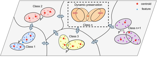
As a result, we can learn the multiple centroids and covariance matrices incrementally for each class. As shown in Figure 1, by using multiple centroids characterizing each class to do inference, we can mitigate the negative effect to the predictive performance caused by the shift between train and test latent representations for further improving the predictive performance.

Another complementary component of our proposed approach is the dynamic preservation, performed dynamically across incoming data streams. This component is designed to make latent representations of data in the classes of both old and new tasks more condensed themselves and more separate to increase the class discrimination ability. More interestingly, this makes the feature extractor a contraction behavior, which helps reduce the discrepancy in the latent representations of the replay memory and the entire old data (cf. Figure 1) for mitigating the catastrophic forgetting.

Finally, we name our proposed approach Class Increamental Learning with Optimal Transport based Mixture Model (CLOT) and conduct comprehensive experiments on the real-world datasets to compare our CLOT with state-of-the-art baselines. The experimental results show that CLOT significantly outperforms state-of-the-art baselines.

To sum up, our work has the following contributions:

• This is the first work that leverages with the rich theoretical body of optimal transport to propose a novel OT-MM for tacking the multimodality of incoming data streams in the OCL scenario.

• Our proposed Dynamic Preservation component that strengthens the class discrimination ability and reduces the gap between train and test latent representations for relieving the catastrophic forgetting. This component is complimentary to OT-MM for devising our CLOT.

• We conduct extensive experiments on the real-world datasets to show that our proposed method performs significantly better than other existing methods.

2 Related work

Figure 2: $t$-SNE visualization on MNIST: Motivation of OT-MM. Left: the test latent representation of CoPE [8] with one centroid (i.e., visualized by digits) per class. Right: the test latent representation of our CLOT with four centroids per class (i.e., visualized by digits). We observe that there exists a shift between the test and train representations. Therefore, centroids learned on the training set might mismatch the testing set. However, using more centroids per class as in our CLOT can relieve this mismatch.

Previous works attempt to tackle the problem of catastrophic forgetting by efficiently designing the training process in a number of ways. Memory-based approaches utilize episodic memory to store past data [32, 4, 5, 33] or employ deep generative models [37, 19] to produce pseudo samples from the previous history. Architecture-based methods dynamically allocate a separate subnetwork for each task [27, 42] to maintain the knowledge of old tasks. Regularization-based approaches encourage important parameters of old tasks to lie in their close vicinity [17, 51, 49] by penalizing their changes. Among these three main lines of work, our method falls into the memory-based approach category, which utilizes the advantages of buffer memory to preserve the discriminative characteristics of data.

Current CL algorithms are often assessed in an incremental classification scenario, where tasks or classes arrive at different timestamps. We here consider the online class-incremental (OCL) setting, which is more realistic but also more challenging. In particular, in comparison to task-incremental learning, the data stream is no longer divided into tasks with clear boundaries. We also have to deal with catastrophic forgetting without any information about the task id that the data come from at both training and inference time. The recent work in OCL usually focuses on: either (i) how to choose meaningful, diverse samples to store [6, 35], also how to select old samples to replay [29], or (ii) how to learn representation effectively [11, 3] , mostly inspired by contrastive learning, (iii) how to solve bias problem for single categorical head [14, 44, 52]. In this work, we present a memory-based learning strategy, also inspired by contrastive learning. However, not only that, we bring a breeze when introducing the theory of optimal transport into continuous learning for the first time. Specifically, an optimal transport-based mixing model will be applied in the online scenario to learn the multiple centroids that characterize each class. Then these centroids will be used to make more accurate predictions and improve episodic memory.

3 Preliminaries

In what follows, we present the background of Wasserstein (WS) distance and optimal transport theory that is necessary for the development of our proposed method.

3.1 Optimal transport and Wasserstein distance

Consider two distributions $\mathbb{P}$ and $\mathbb{Q}$ which operate on the domain $\Omega\subseteq\mathbb{R}^{d}$, let $d\left(\boldsymbol{x},\boldsymbol{y}\right)$ be a non-negative and continuous cost function or metric. Wasserstein distance [34, 40] between $\mathbb{P}$ and $\mathbb{Q}$ w.r.t the metric $d$ is defined as

$$\mathcal{W}_{d}\left(\mathbb{Q},\mathbb{P}\right):=\min_{\gamma\in\Gamma\left(\mathbb{Q},\mathbb{P}\right)}\mathbb{E}_{\left(\boldsymbol{x},\boldsymbol{y}\right)\sim\gamma}\left[d\left(\boldsymbol{x},\boldsymbol{y}\right)\right],$$ (1)

where $\gamma$ is a coupling that admits $\mathbb{Q},\mathbb{P}$ as its marginals.

3.2 Entropic dual-form for OT and WS distance

To enable the application of optimal transport in machine learning and deep learning, [9] developed an entropic regularized dual form. First, they proposed to add an entropic regularization term to primal form (1)

$$\mathcal{W}_{d}^{\varepsilon}\left(\mathbb{Q},\mathbb{P}\right) :=$$

$$\min_{\gamma\in\Gamma\left(\mathbb{Q},\mathbb{P}\right)} \left\{\mathbb{E}_{\left(\boldsymbol{x},\boldsymbol{y}\right)\sim\gamma}\left[d\left(\boldsymbol{x},\boldsymbol{y}\right)\right]+\varepsilon D_{KL}\left(\gamma\|\mathbb{Q}\otimes\mathbb{P}\right)\right\},$$ (2)

where $\varepsilon$ is the regularization rate, $D_{KL}\left(\cdot\|\cdot\right)$ is the Kullback-Leibler (KL) divergence, and $\mathbb{Q}\otimes\mathbb{P}$ represents the specific coupling in which $\mathbb{Q}$ and $\mathbb{P}$ are independent.

Using Fenchel-Rockafellar theorem, they obtained the following entropic regularized dual form of (2)

$$\mathcal{W}_{d}^{\varepsilon}\left(\mathbb{Q},\mathbb{P}\right) =\max_{\phi}\left\{\int\tilde{\phi}\left(\boldsymbol{x}\right)\mathrm{d}\mathbb{Q}\left(\boldsymbol{x}\right)+\int\phi\left(\boldsymbol{y}\right)\mathrm{d}\mathbb{P}\left(\boldsymbol{y}\right)\right\}$$

$$=\max_{\phi}\left\{\mathbb{E}_{\mathbb{Q}}\left[\tilde{\phi}\left(\boldsymbol{x}\right)\right]+\mathbb{E}_{\mathbb{P}}\left[\phi\left(\boldsymbol{y}\right)\right]\right\},$$ (3)

where $\tilde{\phi}\left(\boldsymbol{x}\right):=-\varepsilon\log\left(\mathbb{E}_{\mathbb{P}}\left[\exp\left\{\frac{-d\left(\boldsymbol{x},\boldsymbol{y}\right)+\phi\left(\boldsymbol{y}\right)}{\varepsilon}\right\}\right]\right)$.

4 Our Proposed Method

In this section, we present the details of our proposed method. We start with the general framework and our motivations, followed by the technical details of online mixture model based on optimal transport theory and the simple yet but effective dynamic preservation technique that assists the model in maintaining the performance on the old tasks.

4.1 General Framework and Motivations

In the context of the online class incremental learning, at a time step, our system receives a batch of data examples $X=[X^{c}]_{c\in\mathcal{C}_{new}}$ from a new task, where $\mathcal{C}_{new}$ represents the classes in the new task and $X^{c}$ is the batch data for the class $c$. To mitigate catastrophic forgetting, we also maintain a replay memory $\mathcal{M}$ of the old tasks. We sample a batch of data examples from the replay memory $\bar{X}=[\bar{X}^{c}]_{c\in\mathcal{C}_{old}}$, where $\mathcal{C}_{old}$ represents the classes in the old tasks and $\bar{X}^{c}$ is the batch data for the class $c$ in the replay memory.

We feed $X$ and $\bar{X}$ to the feature extractor $f_{\boldsymbol{\theta}}$ to obtain the batches of latent representations $Z=f_{\boldsymbol{\theta}}(X)$ and $\bar{Z}=f_{\boldsymbol{\theta}}(\bar{X})$ for new and old tasks respectively. For the batches of $X$ and $\bar{X}$, we first perform dynamic preservation to make the classes in the old and new tasks to become more condensed themselves and more separate to each other. By doing this, we hope to strengthen the class discrimination ability for both old and new classes, hence maximally preserving the performance on the old tasks. Subsequently, given the separation of the classes in the old and new tasks, we perform OT-MM which incrementally estimates a mixture model, using optimal transport, for each class to tackle the complexity of incoming data streams.

Algorithm 1 summarizes the main steps of our method which is Class Increamental Learning with Optimal Transport based Mixture Model (CLOT). Additionally, the key motivations of our approach are presented in Figure 1. In what follows, we present and discuss the technicality of dynamic preservation and OT-MM.

Algorithm 1 CLOT

Input: The batches $X=[X^{c}]_{c\in\mathcal{C}_{new}}$ and $\bar{X}=[\bar{X}^{c}]_{c\in\mathcal{C}_{old}}$.
Output: Feature extractor $f_{\boldsymbol{\theta}}$, the centroids/ covariance matrices $[\boldsymbol{\mu}^{c}_{k},\Sigma^{c}_{k}]_{k=1}^{K}$ for each class $c$

1:  Initialize replay memory $\mathcal{M}$

2:  for each batch $(X,\bar{X})$ do

3:     Step 1. Perform dynamic preservation

4:     Step 2. Perform OT-MM

5:     Step 3. Update the replay memory $\mathcal{M}$

6:  end for

4.2 Dynamic Preservation

For each class $c\in\mathcal{C}=\mathcal{C}_{new}\cup\mathcal{C}_{old}$, we maintain an aligned prototype $\boldsymbol{w}^{c}$ to provide the logit to the class $c$ for $\boldsymbol{z}=f_{\boldsymbol{\theta}}(\boldsymbol{x})$ as $\langle\boldsymbol{w}^{c},\boldsymbol{z}\rangle$. To strengthen the separation of the classes in the old and new tasks, we update the feature extractor $f_{\boldsymbol{\theta}}$ and aligned prototypes $\boldsymbol{w}^{c}$ by minimizing the following cross-entropy loss over $X=[X^{c}]_{c\in\mathcal{C}_{new}}$ and $\bar{X}=[\bar{X}^{c}]_{c\in\mathcal{C}_{old}}$:

$$\small{}L_{1}(\boldsymbol{\theta},\boldsymbol{w})=\sum_{c\in\mathcal{C}}\mathbb{E}_{\boldsymbol{x}^{c}\sim X^{c}\text{ or}\,\bar{X}^{c}}\left[-\log\frac{\exp\left\langle\boldsymbol{w}^{c},f_{\boldsymbol{\theta}}\left(\boldsymbol{x}^{c}\right)\right\rangle}{\sum_{c^{\prime}}\exp\left\langle\boldsymbol{w}^{c^{\prime}},f_{\boldsymbol{\theta}}\left(\boldsymbol{x}^{c}\right)\right\rangle}\right].$$ (4)

After solving the above optimization problem (4), the representation of the classes become more separating. We then compute the mean prototypes $\boldsymbol{p}^{c}$ for each class $c$ as the average of the latent representations, i.e.,

$$\boldsymbol{p}^{c}=\begin{cases}\frac{1}{|X^{c}|}\sum_{\boldsymbol{x}^{c}\in X^{c}}f_{\boldsymbol{\theta}}\left(\boldsymbol{x}^{c}\right)&c\in\mathcal{C}_{new}\\ \frac{1}{|\bar{X}^{c}|}\sum_{\boldsymbol{x}^{c}\in\bar{X}^{c}}f_{\boldsymbol{\theta}}\left(\boldsymbol{x}^{c}\right)&c\in\mathcal{C}_{old}\end{cases},$$ (5)

where $|\cdot|$ returns the cardinality of a set.

To encourage the representations of the class $c$ to be pulling around its mean prototype and the representations of other classes $c^{\prime}\neq c$ to be pushing away the mean prototype $\boldsymbol{p}^{c}$, we propose to minimize the following loss function:

$$\small{}L_{2}(\boldsymbol{\theta})=\sum_{c\in\mathcal{C}}\mathbb{E}_{\boldsymbol{x}^{c}\sim X^{c}\text{ or}\,\bar{X}^{c}}\left[-\log\frac{\exp\left\{-\|f_{\boldsymbol{\theta}}\left(\boldsymbol{x}^{c}\right)-\boldsymbol{p}^{c}\|_{2}^{2}\right\}}{\sum_{c^{\prime}}\exp\left\{-\|f_{\boldsymbol{\theta}}\left(\boldsymbol{x}^{c}\right)-\boldsymbol{p}^{c^{\prime}}\|_{2}^{2}\right\}}\right]$$ (6)

After performing the dynamic preservation, the latent representations of the classes in the old and new tasks become more condensed themselves and more separate from each other. Resultantly, we increase the class discrimination ability for those in the old and new tasks. Additionally, the feature extractor $f_{\boldsymbol{\theta}}$ has a contraction behavior which helps reduce the shift in the latent representations of the data examples in the old tasks and those in the replay memory. Summarily, we expect that the increasing class discrimination ability and the contracting feature extractor aid CLOT to mitigate the catastrophic forgetting (cf. Figure 1). The key steps of the dynamic preservation is summarized in Algorithm 2.

Algorithm 2 Dynamic preservation

Input:The batches $X=[X^{c}]_{c\in\mathcal{C}_{new}}$ and $\bar{X}=[\bar{X}^{c}]_{c\in\mathcal{C}_{old}}$
Output:The feature extractor $f_{\boldsymbol{\theta}}$

1:  Update $\boldsymbol{w}^{c\in\mathcal{C}},\boldsymbol{\theta}$ by minimizing (4).

2:  Compute the mean prototypes using (5).

3:  Update $\boldsymbol{\theta}$ by minimizing (6).

We observe that though becoming more condensed and separate, the latent representations of data streams in the new task and replay memory are still sufficiently complex with multi-modality. Therefore, we propose an online OT-based mixture model (OT-MM) approach to incrementally learn the mixture model for each class.

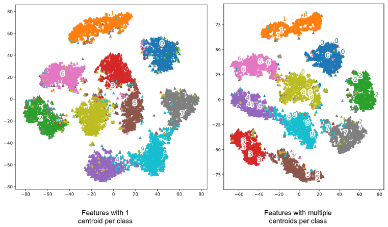
Mixture models enable our OT-MM to use multiple centroids to characterize a class in the online learning manner. Figure 2 demonstrates the advantages of using multiple centroids to characterize a class. Specifically, we use t-SNE to visualize the test latent representations of CoPE [8] using one centroid per class and our CLOT using four centroids per class. We observe that there exists a shift between test and train representations. Hence, the centroids tailored to the train set might mismatch the test set. However, it can be seen that using more centroids per class as in our CLOT can mitigate this mismatch. Together with the possibly complex distribution of incoming data streams, this is another motivation for our OT-MM.

Figure 3: Average Accuracy by different number of centroids per class (CIFAR10).

Figure 4: Average accuracy through tasks.

4.3 Optimal transport based mixture model

4.3.1 The Derivation of OT-MM

OT-MM is one important building-block of our framework. Given a class $c\in\mathcal{C}$ of an old or a new task, we aim to use the mature theoretical body of OT to develop the online OT-MM for data in this class in the sense that the centroids and covariance matrices of the mixture model are incrementally updated according to incoming data streams.

Given the latent representations or feature vectors of the class $c$: $D_{c}=\left\{\boldsymbol{z}_{1}^{c},...,\boldsymbol{z}^{c}_{N_{c}}\right\}$, wherein each $\boldsymbol{z}_{i}^{c}=f_{\boldsymbol{\theta}}(\boldsymbol{x}_{i}^{c})$ is the latent representation or feature vector of data example $\boldsymbol{x}_{i}^{c}$ via the feature extractor $f_{\boldsymbol{\theta}}$. We denote $\mathbb{P}_{c}:=\frac{1}{N_{c}}\sum_{i=1}^{N_{c}}\delta_{\boldsymbol{z}_{i}^{c}}$ as the empirical data distribution over all data of the class $c$ appearing in all data streams on the latent space. When data are arriving in streams, we need to learn a Gaussian mixture model (GMM) that approximates the data distribution $\mathbb{P}_{c}$. Consider the following GMM

$$\mathbb{Q}_{c}:=\sum_{k=1}^{K}\pi_{k,c}\mathcal{N}\left(\boldsymbol{\mu}_{k,c},\text{diag}\left(\mathbf{\sigma}_{k,c}^{2}\right)\right),$$

where $\boldsymbol{\pi}^{c}=\left[\pi_{k,c}\right]_{k=1}^{K}$ represents mixing proportions and $\boldsymbol{\mu}_{k,c},\text{diag}\left(\mathbf{\sigma}_{k,c}^{2}\right)$ are the mean vector and covariance matrix of the $k$-th Gaussian. To learn this GMM, we propose minimizing a WS distance between $\mathbb{P}_{c}$ and $\mathbb{Q}_{c}$ as

$$\min_{\boldsymbol{\pi}^{c},\boldsymbol{\mu}^{c},\Sigma^{c}}\mathcal{W}_{d}\left(\mathbb{P}_{c},\sum_{k=1}^{K}\pi_{k,c}\mathcal{N}\left(\boldsymbol{\mu}_{k,c},\text{diag}\left(\mathbf{\sigma}_{k,c}^{2}\right)\right)\right),$$

where $\boldsymbol{\pi}^{c}=\left[\pi_{k,c}\right]_{k=1}^{K}$, $\boldsymbol{\mu}^{c}=\left[\boldsymbol{\mu}_{k,c}\right]_{k=1}^{K}$, $\Sigma^{c}=\left[\text{diag}\left(\mathbf{\sigma}_{k,c}\right)\right]_{k=1}^{K}$, and $d$ is a distance on the latent space.

To handle the above WS distance, we need the parameterized samples $\tilde{\boldsymbol{z}}^{c}$ from the GMM or $\tilde{\boldsymbol{z}}^{c}\sim\mathbb{Q}_{c}=\sum_{k=1}^{K}\pi_{k,c}\mathcal{N}\left(\boldsymbol{\mu}_{k,c},\text{diag}\left(\mathbf{\sigma}_{k,c}^{2}\right)\right)$. To this end, we first sample $\tilde{\boldsymbol{z}}_{k}^{c}\sim\mathcal{N}\left(\boldsymbol{\mu}_{k,c},\text{diag}\left(\mathbf{\sigma}_{k,c}^{2}\right)\right)$ by using the reparameterization trick

$$\tilde{\boldsymbol{z}}_{k}^{c}=\boldsymbol{\mu}_{k,c}+\boldsymbol{\epsilon}_{k}\text{diag}\left(\mathbf{\sigma}_{k,c}\right),$$

where the source of randomness $\boldsymbol{\epsilon}_{k}\sim\mathcal{N}\left(\mathbf{0},\mathbb{I}\right)$. We then sample the one-hot vector $\boldsymbol{y}\sim\text{Cat}\left(\boldsymbol{\pi}^{c}\right)$ and compute

$$\tilde{\boldsymbol{z}}^{c}=\sum_{k=1}^{K}y_{k}\tilde{\boldsymbol{z}}_{k}^{c}=\sum_{k=1}^{K}y_{k}\left(\boldsymbol{\mu}_{k,c}+\boldsymbol{\epsilon}_{k}\text{diag}\left(\mathbf{\sigma}_{k,c}\right)\right).$$

To do a continuous relaxation [15] of $\boldsymbol{y}$ for enabling learning $\boldsymbol{\pi}^{c}$, we parameterize $\boldsymbol{\pi}^{c}=\text{softmax}\left(\boldsymbol{\alpha}^{c}\right)$ and compute

$$y_{k} =\frac{\exp\left\{\left(\log\pi_{k,c}+G_{k}\right)/\tau\right\}}{\sum_{j=1}^{K}\exp\left\{\left(\log\pi_{j,c}+G_{j}\right)/\tau\right\}},k=1,...,K$$

$$\tilde{\boldsymbol{z}}^{c} =\sum_{k=1}^{K}y_{k}\tilde{\boldsymbol{z}}_{k}^{c}=\sum_{k=1}^{K}y_{k}\left(\boldsymbol{\mu}_{k,c}+\boldsymbol{\epsilon}_{k}\text{diag}\left(\mathbf{\sigma}_{k,c}\right)\right),$$

where $\tau>0$ is a temperature parameter and random noises $G_{k}$ are i.i.d. sampled from Gumbel distribution (i.e., $G_{k}=-\log\left(-\log u_{k}\right)$ for $u_{k}\sim\text{Uniform}(0;1)$).

To train the WS distance of interest, we use the $\varepsilon$-entropic dual-form [9] (cf. Section 3.2) as

$$\mathcal{W}^{\varepsilon}_{d}\left(\mathbb{P}_{c},\sum_{k=1}^{K}\pi_{k,c}\mathcal{N}\left(\boldsymbol{\mu}_{k,c},\text{diag}\left(\mathbf{\sigma}_{k,c}^{2}\right)\right)\right)$$

$$=\max_{\phi}\left\{\mathbb{E}_{\mathbb{P}_{c}}\left[\phi\left(\boldsymbol{z}^{c}\right)\right]+\mathbb{E}_{\mathbb{Q}_{c}}\left[\tilde{\phi}\left(\tilde{\boldsymbol{z}}^{c}\right)\right]\right\},$$ (7)

where $\varepsilon>0$ is a small number, $\phi$ is the Kantorovich network, $\tilde{\boldsymbol{z}}^{c}=\sum_{k=1}^{K}y_{k}\left(\boldsymbol{\mu}_{k,c}+\boldsymbol{\epsilon}_{k}\text{diag}\left(\mathbf{\sigma}_{k,c}\right)\right)$, and

$$\tilde{\phi}\left(\tilde{\boldsymbol{z}}^{c}\right)=-\varepsilon\log\left(\mathbb{E}_{\mathbb{P}_{c}}\left[\exp\left\{\frac{-d\left(\boldsymbol{z}^{c},\tilde{\boldsymbol{z}}^{c}\right)+\phi\left(\boldsymbol{z}^{c}\right)}{\varepsilon}\right\}\right]\right).$$

4.3.2 OT-MM in Online Continual learning Scenario

We now present how to perform our OT-MM in the online continual learning scenario when we need to update the set of centroids and covariance matrices for a class $c\in\mathcal{C}$ based on the batch $X^{c}$ or $\bar{X}^{c}$. Looking into Eq. (7), this objective function is in the form of expectation, hence perfectly fitting for online learning. Specifically, we use the current batch $X^{c}$ or $\bar{X}^{c}$ for each class $c$ to solve

$$\min_{\boldsymbol{\pi}^{c},\boldsymbol{\mu}^{c},\Sigma^{c}}\max_{\phi}\left\{\mathbb{E}_{X^{c}\,or\,\bar{X}^{c}}\left[\phi\left(f_{\boldsymbol{\theta}}(\boldsymbol{x}^{c})\right)\right]+\mathbb{E}_{\mathbb{Q}_{c}}\left[\tilde{\phi}\left(\tilde{\boldsymbol{z}}^{c}\right)\right]\right\}.$$ (8)

To solve the optimization problem (8), we update the Kantorovich network $\phi$ several times and then update the mixing propotions $\boldsymbol{\pi}^{c}$, the set of centroids $\boldsymbol{\mu}^{c}$, and the set of covariance matrices $\Sigma^{c}$ for class $c$ in several times.

The key steps of OT-MM is summarized in Algorithm 3. Eventually, we harvest the centroids $[\boldsymbol{\pi}^{c}]_{c\in\mathcal{C}}$ and covariance matrices $[\Sigma^{c}]_{c\in\mathcal{C}}$ to select diverge replay memory for a task and do inference in the testing phase (cf. Section 4.4).

Algorithm 3 OT-GMM in the OCL scenario

Input:The batches $X=[X^{c}]_{c\in\mathcal{C}_{new}}$ and $\bar{X}=[\bar{X}^{c}]_{c\in\mathcal{C}_{old}}$
Output:$[\boldsymbol{\pi}^{c},\boldsymbol{\mu}^{c},\Sigma^{c}]_{c\in\mathcal{C}}$

1:  for  each $c\in\mathcal{C}$ do

2:     Update $\phi$ according to (8).

3:     Update $[\boldsymbol{\pi}^{c},\boldsymbol{\mu}^{c},\Sigma^{c}]$ according to (8).

4:  end for

Method	M = 1k	M = 3k	M = 5k	M = 0.2k	M = 0.5k	M = 1k	M = 0.1k	M = 0.5k	M = 1.5k
iid-offline	$50.28\pm 0.66$	$50.28\pm 0.66$	$50.28\pm 0.66$	$83.02\pm 0.60$	$83.02\pm 0.60$	$83.02\pm 0.60$	$98.44\pm 0.02$	$98.44\pm 0.02$	$98.44\pm 0.02$
iid-online	$20.10\pm 0.90$	$20.10\pm 0.90$	$20.1\pm 0.90$	$62.31\pm 1.67$	$62.31\pm 1.67$	$62.31\pm 1.67$	$96.57\pm 0.14$	$96.57\pm 0.14$	$96.57\pm 0.14$
DVC [11]	$\mathbf{10.93\pm 0.49}$	$14.49\pm 0.90$	$20.83\pm 0.89$	$28.56\pm 2.10$	$34.92\pm 2.27$	$45.02\pm 2.72$	_	_	_
OCD [18]	$3.71\pm 0.5$	$9.2\pm 0.21$	$11.56\pm 0.32$	$15.83\pm 2.30$	$21.02\pm 5.24$	$26.45\pm 2.40$	_	_	_
MIR [1]	$8.20\pm 0.72$	$14.9\pm 0.40$	$20.00\pm 0.57$	$24.3\pm 2.01$	$35.6\pm 2.56$	$42.80\pm 2.22$	$73.6\pm 0.50$	$86.5\pm 0.22$	$91.2\pm 0.36$
OCS [50]	$8.50\pm 0.35$	$13.76\pm 0.70$	$19.98\pm 0.65$	_	_	_	_	_	_
ASER [36]	$9.60\pm 0.88$	$13.08\pm 0.87$	$15.00\pm 0.64$	$22.38\pm 2.94$	$26.42\pm 4.80$	$30.67\pm 3.10$	$58.02\pm 0.07$	$75.47\pm 0.04$	$85.68\pm 0.03$
Reservoir [41]	$8.60\pm 1.58$	$13.5\pm 2.61$	$19.60\pm 0.53$	$25.96\pm 1.41$	$33.85\pm 1.76$	$40.531\pm 5.30$	$69.22\pm 1.15$	$86.50\pm 1.04$	$91.27\pm 0.96$
GDUMB [28]	$8.48\pm 0.26$	$11.24\pm 0.56$	$15.63\pm 0.60$	$24.60\pm 1.50$	$28.70\pm 0.63$	$33.24\pm 2.10$	$73.5\pm 0.12$	$86.16\pm 0.01$	$92.07\pm 0.01$
CoPE [8]	$9.22\pm 0.55$	$15.15\pm 0.50$	$19.56\pm 1.22$	$37.20\pm 1.80$	$42.22\pm 0.54$	$47.98\pm 2.62$	$72.57\pm 2.10$	$88.92\pm 0.99$	$92.50\pm 0.33$
CLOT (Ours)	$10.62\pm 0.45$	$\mathbf{15.80\pm 0.55}$	$\mathbf{22.35\pm 0.40}$	$\mathbf{42.28\pm 0.50}$	$\mathbf{50.08\pm 1.00}$	$\mathbf{54.45\pm 1.20}$	$\mathbf{77.40\pm 0.21}$	$\mathbf{90.98\pm 0.35}$	$\mathbf{93.71\pm 0.05}$
	a) CIFAR-100			b) CIFAR-10			c) MNIST

Table 1: Average Accuracy (higher is better), M denotes the memory buffer size. All numbers are the average of 5 runs. The data in the table represents Average Accuracy ± standard deviation.

4.4 Replay memory selection and inference process

We now present how to utilize the output of the OT-MM for selecting the replay memory of the new task and how to do inference.

Replay memory selection:

After processing each batch $(X,\bar{X})$, as shown in Step 3 (Line 5) in Algorithm 1, we select some more data points to supplement the replay memory of the new task as follows:

• For a centroid of a class, we choose some closest data points of this class in the current batch to add to the replay memory.

• If the replay memory is full, we randomly pick some data points in the current replay memory to replace by the fresh-new ones.

Doing inference:

Given an unseen data point $\boldsymbol{x}$, we compute the distance of $\boldsymbol{x}$ to each class $c$ and classify $\boldsymbol{x}$ to the closest class as follows:

$$\hat{y}=\arg\min_{c\in\mathcal{C}}d\left(\boldsymbol{x},c\right)\text{ where }d\left(\boldsymbol{x},c\right)=\min_{k\leq K}d(f_{\boldsymbol{\theta}}\left(\boldsymbol{x}\right),\boldsymbol{\mu}_{k,c})$$

5 Experiments

In this section, we review the experimental settings including datasets, baselines, and metrics used to compare our method against other state-of-the-art models. We then report and analyse the results to validate the effectiveness of our approach.

5.1 Experimental setup

Datasets: We use three benchmark datasets including:

• Split-MNIST is constructed by splitting the MNIST dataset (with 60k training samples) into 5 disjoint subsets, corresponding to 5 tasks, each of which consists of 2 classes.

• Split-CIFAR10 is constructed by splitting CIFAR10 dataset into 5 disjoint tasks, hence each task has 2 different classes.

• Split-CIFAR100 is a variant CL dataset constructed from CIFAR100 where 50k training samples of 100 classes is divided into 20 tasks of 5 classes.

Architectures: For the experiments on Split-MNIST dataset, we use a simple MLP neural network with 2 hidden layers of 400 units. While a slim-version of ResNet-18 will be used to evaluate on Split-CIFAR10 and Split-CIFAR100.

Baselines: We use several state-of-the-art methods in Continual learning, specifically in Online Continual Learning (OCL), to compare with our proposed method.

• iid-online and iid-offline: give the performance when ignoring the challenges of non-stationary data stream in OCL scenarios. Both of them train a model from i.i.d. sampled mini-batches (i.e. there is no change of the distribution of data in the learning process). While iid-online only allows learning once over data, iid-offline allows a model to be trained from multiple epochs.

• Regarding the recent methods for OCL, the chosen baselines can divided into 2 main groups. The first group focuses on improving the quality of replay memory: Reservoir, OCS (ICRL2022), MIR (NeurIPS2019) are well-known techniques to build memory buffer, GDumb (ECCV2020) is interested in the way to retrieve data more effectively, while ASER (AAAI2021) consider both updating and retrieving data from memory. The second group includes the methods that help improve a model mainly through more effective representation learning: DVC (CVPR2022), OCD (IJICAI2022), CoPE (ICCV2021).

5.2 Performance comparison

Figure 5: Features on latent space of our method (a and b) and CoPE (c). It can be observed that 4 centroids is better than 1 centroid. CLOT 1-centroid is better than CoPE 1-centroid due to the effect of the dynamic preservation for learning better latent representations.

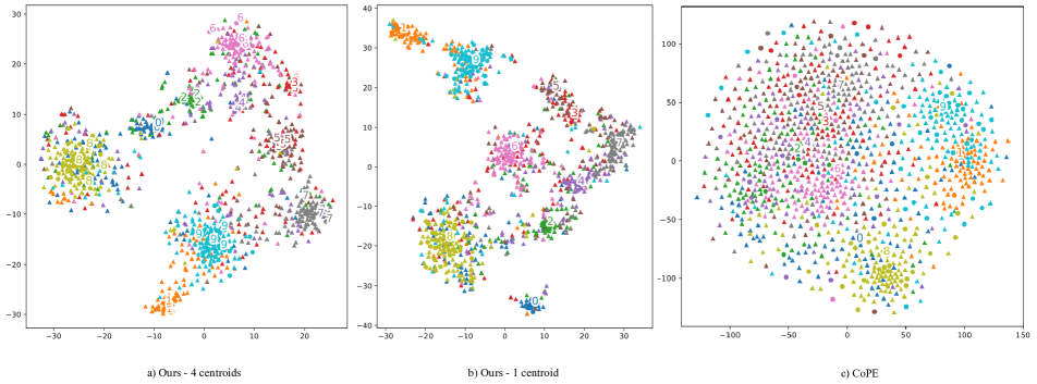
Table 1 summarizes the experimental results on three datasets with various memory sizes. On MNIST, we compare our method with five baselines and achieve better results. Especially when memory sizes are small (0.1k), we exceed the strongest baseline (MIR) by roughly 4%. On CIFAR10, CLOT again outperforms the SOTA baselines. The largest gap between CLOT and the best baseline is around 8%. On CIFAR100, the memory size for each class and the batch size in each learning step both are very small, making this the most challenging dataset to learn. The results show that with a sufficient large memory size (3k, 5k), our CLOT surpasses the baselines, while with a too-small memory size, our CLOT is the runner-up method.

Among three datasets, the superiority of CLOT is most apparent in CIFAR10. This because that MNIST is a fairy easy dataset, especially when the memory is large enough to get the representational diversity of the old samples. Thus, for the results on MNIST with memory size 1.5K, the methods do not show clear performance differences. As for CIFAR100, we can see that our method needs a sufficient amount of data to show its strengths in learning representation. Because with too small memory size and batch size, some samples from all classes are not always available.

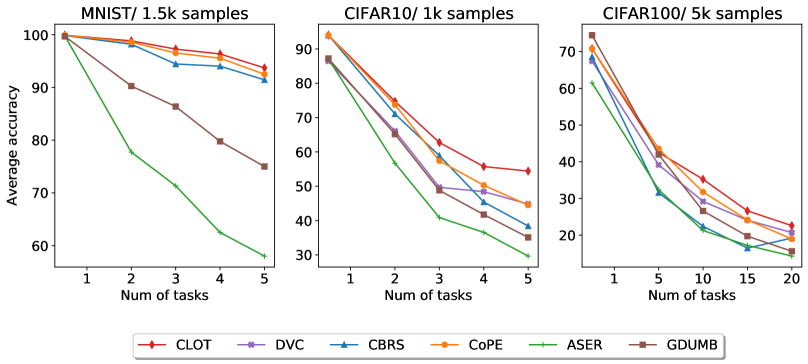
Figure 4 shows the visual results about the average accuracy on observed tasks of the different methods with the large enough memory size on each dataset. It is easy to see that our method outperforms the other baselines, especially as the number of tasks increases. This is most evident in CIFAR10, consistent with the reasons discussed earlier.

5.3 Ablation study

In what follows, we present additional experimental results to analyse the effectiveness of components in CLOT.

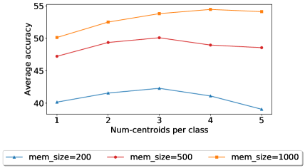
The role of using multiple centroids in general: For our OT-MM, we examine the influence of number of centroids per class. Figure 3 depicts the curves of average accuracies on CIFAR10 when Num-centroids varies. We observe that in all cases, the performance improves when we increase the number of centroids per class from 1 to a certain threshold. The bigger the memory size is, the bigger the threshold is. Moreover, if these thresholds are exceeded, the model performance depends on the support level of replay memory: the smaller memory size leads to the lower the representation learning quality, and higher prediction error. When memory size = 0.2K, if the number of centroids is bigger than 3, the model performance degrades most. On the other hand, with a larger memory size (e.g., memory size = 1K), the ideal number of centroids is 4, and when increasing the number of centroids to 5, the model quality does not degrade significantly. Therefore, it can be seen that our prediction method using many centroids would achieve the best results when there is a harmonious combination with the representation learning quality.

The role of centroids in improving replay buffer: In our framework, we leverage centroids learned from OT-MM to improve the quality of the memory buffer. Table 2 is an ablation study on the effect of using or not using centroids to select samples for the replay buffer. It can be observed that in all cases, using centroids to select samples consistently offers better results than not using centroids. Regardless that the sample selection based on centroids is quite simple, the results support our intuition that centroids help effectively characterize data and improve the diversity in the episode memory.

	Num of centroids
	1	2	3	4	5	8
Use centroids	50.1	52.5	53.8	54.5	54.1	54
w/o centroids	50.1	52.11	53.2	54.0	53.6	53.3

Table 2: Effect of using centroids on replay memory selection. We compare the performance when using centroids to select samples (Use centroids) and when selecting samples at random for the replay memory (w/o centroids).

The role of centroids in prediction: To verify the role of using multiple centroids when making decisions, we present $t$-SNE visualization (Figure 5) of the feature space of a setting on CIFAR10. Figures 5a and 5b illustrate our approach when using multiple centroids and only 1 centroid when predicting. We can see that, in the real scenario, the features of the classes are usually distributed with multi-modality. Therefore, using more centroids helps to characterize more accurately multi-modal distributions, thus generally giving better prediction than using only 1 centroid.

Furthermore, Figure 5c illustrates the corresponding results on latent space using CoPE where the features of different classes are not well separated and each class has only one centroid for prediction. When comparing 5c with 5a and 5b, we again emphasize the effectiveness of our framework in improving the quality of representation learning via dynamic preservation, along with making decisions based on multiple centroids produced by OT-MM.

6 Conclusion

In this work, we have proposed a novel method for Online CIL scenarios, which is for the first time that OT theory has been leveraged with Continual learning. We have introduced a new perspective that helps the network to make predictions based on many centroids for each class of data to tackle more efficiently their multi-modality. In addition, we have further proposed a strategy of remembering old knowledge flexibly, called Dynamic Preservation, which complements to the prediction mechanism above. Furthermore, the extensive experiments on three commonly used benchmark datasets demonstrate the effectiveness of our method.

7 Supplementary Material

7.1 Implementation Detail

We implement our proposed method and baselines on the same code base, based on the learner-evaluator framework proposed in [8]. Our code is available at https://github.com/tranquyenbk173/Streaming_WSD_GGM

7.1.1 Hyperparameters configuration

We shared the same replay memory size (total samples of all classes) per dataset for each method, and set the batch size for all methods to 10, the size of the retrieved batch is the same as the batch size from data stream. The optimizers are all SGD, the learning rate and other hyperparameters were trying to adjust to get the best results for each method. In addition to that, for a fair comparison, the classes in each task and the order of tasks are fixed in all experiments of the same kind. Table 3 presents the setting.

Hyper-params	Split	Split	Split
	CIFAR100	CIFAR10	MNIST
batch_size	10	10	10
memory size	[ 1k, 3k, 5k ]	[ 0.2k, 0.5k, 1k ]	[ 0.1k, 0.5k, 1.5k ]

Table 3: Shared Hyperparameter configurations among our method and baselines for three datasets.

7.1.2 Evaluation and metrics

In all experiments, we use a single-head architecture, where the final classifier layer is shared across all the tasks (except for CLOT and CoPE, only features extractor is available), and the task identity is not provided during inference.

Following the CL literature [4, 25], we used the following metrics to evaluate:

• Average accuracy ($\mathcal{A}_{T}$): Averaged test accuracy of all tasks after completing learning T task.

  $$\mathcal{A}_{t}=\frac{1}{T}\sum_{j=1}^{T}a_{T,j},$$

  where $a_{i,j}$ is the performance of the model on the held-out testing set of task $j$ after the model is trained from task $1$ to $i$.

• Average forgetting ($\mathcal{F}_{T}$): The averaged gap between the highest recorded and final task accuracy at the end of continual learning on $T$ tasks.

  $$\mathcal{F}_{T}=\frac{1}{T-1}\sum_{j=1}^{T-1}f_{T,j},$$

  where $f_{i,j}=\max_{l\in\{1,...,i-1\}}a_{l,j}-a_{i,j}$

7.2 Additional Experiments

7.2.1 Average forgetting

Table 4 shows the average forgetting at the end of data stream of methods on 3 datasets. Our CLOT is the method with the lowest average forgetting in most cases. The most enormous difference is shown on the MNIST dataset, with a gap of about 6 % from the most robust baseline (MIR). On the CIFAR10, CLOT avoids forgetting better than the best method by more than 2.6%. With the most challenging dataset - CIFAR100, our method also shows an advantage over other methods.

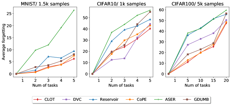
On the other hand, Figure 6 depicts the average accuracy of methods through tasks. We can see that, in general, CLOT is the method with the lowest forgetting rate (on the MNIST and CIFAR100 datasets) / or in the group with the least forgetting rate (on the CIFAR10 set) during the continual learning process. At the end of the data stream, our proposed method shows a clear difference in avoiding catastrophic forgetting compared to the baselines on the two datasets: MNIST and CIFAR10.

These evidences once again confirm the effectiveness of our framework in online continual learning scenario.

Figure 6: Average forgetting through tasks. Lower is better.

Method	M = 1k	M = 3k	M = 5k	M = 0.2k	M = 0.5k	M = 1k	M = 0.1k	M = 0.5k	M = 1.5k
DVC [11]	$\mathbf{52.25\pm 0.41}$	$51.69\pm 0.34$	$50.36\pm 0.46$	$60.15\pm 5.5$	$55.2\pm 5.99$	$44.37\pm 1.21$	_	_	_
OCD [18]	$68.55\pm 1.5$	$65.33\pm 0.78$	$64.1\pm 0.57$	$68.48\pm 4.41$	$62.34\pm 7.59$	$51.09\pm 1.62$	_	_	_
MiR [1]	$58.862\pm 0.97$	$56.56\pm 0.81$	$54.55\pm 0.72$	$58.23\pm 4.3$	$56.65\pm 1.6$	$46.34\pm 3.2$	$33.2\pm 2.59$	$16.01\pm 1.51$	$8.87\pm 1.8$
OCS [50]	$60.01\pm 1.81$	$57.22\pm 0.55$	$56.88\pm 0.6$	_	_	_	_	_	_
ASER [36]	$58.71\pm 0.84$	$59.44\pm 0.92$	$59.67\pm 0.79$	$62.05\pm 3.2$	$60.01\pm 1.73$	$56.67\pm 3.27$	$40.55\pm 3.12$	$20.53\pm 2.52$	$25.4\pm 0.25$
Reservoir [41]	$58.91\pm 1.7$	$56.70\pm 0.5$	$55.88\pm 0.87$	$57.62\pm 2.45$	$52.25\pm 1.41$	$48.53\pm 2.3$	$35.58\pm 2.5$	$15.69\pm 2.1$	$9.48\pm 1.13$
GDUMB [28]	$59.11\pm 1.17$	$57.83\pm 0.82$	$56.55\pm 0.66$	$57.88\pm 1.89$	$57.15\pm 2.1$	$55.16\pm 1.55$	$33.5\pm 2.89$	$12.66\pm 0.2$	$8.12\pm 0.93$
CoPE [8]	$55.17\pm 0.3$	$54.65\pm 0.45$	$48.47\pm 0.99$	$52.35\pm 2.15$	$49.76\pm 2.39$	$42.99\pm 2.87$	$34.49\pm 3.62$	$12.915\pm 1.8$	$7.53\pm 1.2$
CLOT (Ours)	$53.21\pm 0.51$	$\mathbf{51.01\pm 0.55}$	$\mathbf{47.59\pm 0.57}$	$\mathbf{51.32\pm 2.3}$	$\mathbf{47.08\pm 3.1}$	$\mathbf{40.25\pm 1.1}$	$\mathbf{27.46\pm 3.17}$	$\mathbf{10.74\pm 0.21}$	$\mathbf{6.27\pm 0.28}$
	a) CIFAR-100			b) CIFAR-10			c) MNIST

Table 4: Average Forgetting (lower is better), M denotes the memory buffer size. All numbers are the average of 5 runs. The data in the table represents Average Forgetting ± standard deviation.

7.2.2 Additional technicalities

Clip grad proportion of prototypes

	Clip grad proportion
	0.0	0.001	0.05	0.08	0.1	0.15	0.5
MNIST	93.22	93.46	93.50	93.58	93.71	93.20	92.80
CIFAR10	53.23	53.55	54.41	54.45	52.40	49.12	46.55

Table 5: Average Accuracy by different clip grad proportion

In the Dynamic Preservation phrase, when solving the problem (4):

$$\small{}L_{1}(\boldsymbol{\theta},\boldsymbol{w})=\sum_{c\in\mathcal{C}}\mathbb{E}_{\boldsymbol{x}^{c}\sim X^{c}\text{ or}\,\bar{X}^{c}}\left[-\log\frac{\exp\left\langle\boldsymbol{w}^{c},f_{\boldsymbol{\theta}}\left(\boldsymbol{x}^{c}\right)\right\rangle}{\sum_{c^{\prime}}\exp\left\langle\boldsymbol{w}^{c^{\prime}},f_{\boldsymbol{\theta}}\left(\boldsymbol{x}^{c}\right)\right\rangle}\right],$$ (4)

we use a secondary technique to control the updating of the prototypes as follows:

• Compute gradient of $L_{1}$ w.r.t prototypes:

  $$g_{\boldsymbol{p}}=\nabla_{\boldsymbol{p}}L_{1}$$

• Adjust the gradient for prototypes: new prototypes are allowed to learn more than old prototypes. With clip grad proportion $\alpha\in\left(0,1\right)$, we update:

  $$\boldsymbol{p^{c}}=\left\{\begin{matrix}\boldsymbol{p}^{c}-\eta*\alpha*g_{\boldsymbol{p}}&c\in\mathcal{C}_{old},\\ \boldsymbol{p}^{c}-\eta*g_{\boldsymbol{p}}&c\in\mathcal{C}_{new}\end{matrix}\right.$$

Clip grad proportion $\alpha$ is a hyperparameter that tells us how much portability we allow for prototypes. Table 5 shows the results when changing the value of clip grad proportion. The experiments on MNIST give the best results with $alpha=0.001$, and the ideal value is $0.08$ on CIFAR10.

In continual learning, the representation of features often shift too much, especially at transition times between tasks. If we learn prototypes arbitrarily without control (especially when the old data reviewed are very limited), they then move to unfavorable locations, making the features of different classes to be unseparated well, on both the training and testing sets. The table also shows that, on all 3 datasets, if the clip grad proportion is too high, the average accuracy is highly reduced. While, if it is too small, the model performance is greatly stable. That is, the features of the old classes are fixedly distributed in some places that is only good for the old tasks, and the new tasks does not have much space to place the new features.

Prototype adjustment

Figure 7: $t$-SNE visualization of learned features and prototypes. The features of different classes are assigned different colors. The prototypes are located in the position of the red ”X” signs.

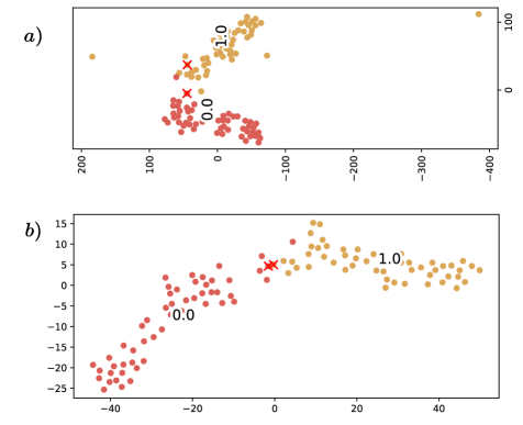
In this section, we conduct additional experiments and explanations regarding why we need to adjust the aligned prototypes to the mean prototypes (a.k.a. the prototype adjustment) when compressing the feature vectors in the dynamic preservation.

Our practical observations show that the aligned prototypes (used to learn feature extractor by some objective functions like Cross Entropy loss) do not often locate at the centre of each class and also very close to each other (Figure 7). This seems to be detrimental. Additionally, in the next update step (6), we immobilize the prototypes to learn the feature extractor so that the features will move to the corresponding prototypes. Therefore, if we use the aligned prototypes directly for (6), the clusters of features (of different classes) will be overlapped. Consequently, the predictive efficiency may be degraded. Moreover, after performing (4), the features of different classes are quite separable. Hinted by this observation, we compute mean prototypes in (5) and use them to solve the optimization problem in (6) for compressing the feature vectors around the corresponding mean prototypes.

Figure 8: Performance of CLOT when adjusting prototypes (Adjust proto) and not (Not adjust proto), according to (5)

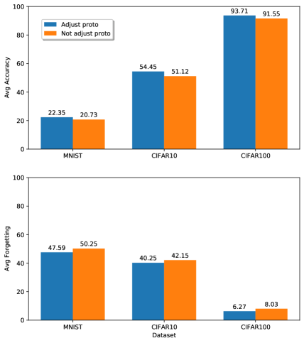
Figure 8 shows the effect of prototype adjustment in (5). We can see this change helps to solve the issue mentioned above and improve the performance. On all 3 datasets, when adjusting the prototypes according to (5), we obtain higher average accuracies and lower average forgetting scores.

References

- [1] Rahaf Aljundi, Eugene Belilovsky, Tinne Tuytelaars, Laurent Charlin, Massimo Caccia, Min Lin, and Lucas Page-Caccia. Online continual learning with maximal interfered retrieval. In H. Wallach, H. Larochelle, A. Beygelzimer, F. d'Alché-Buc, E. Fox, and R. Garnett, editors, Advances in Neural Information Processing Systems 32, pages 11849–11860. Curran Associates, Inc., 2019.
- [2] Adrian Bulat, Jean Kossaifi, Georgios Tzimiropoulos, and Maja Pantic. Incremental multi-domain learning with network latent tensor factorization. In The Thirty-Fourth AAAI Conference on Artificial Intelligence, AAAI 2020, The Thirty-Second Innovative Applications of Artificial Intelligence Conference, IAAI 2020, The Tenth AAAI Symposium on Educational Advances in Artificial Intelligence, EAAI 2020, New York, NY, USA, February 7-12, 2020, pages 10470–10477. AAAI Press, 2020.
- [3] Lucas Caccia, Rahaf Aljundi, Nader Asadi, Tinne Tuytelaars, Joelle Pineau, and Eugene Belilovsky. New insights on reducing abrupt representation change in online continual learning. In The Tenth International Conference on Learning Representations, ICLR 2022, Virtual Event, April 25-29, 2022. OpenReview.net, 2022.
- [4] Arslan Chaudhry, Marc’Aurelio Ranzato, Marcus Rohrbach, and Mohamed Elhoseiny. Efficient lifelong learning with a-GEM. In International Conference on Learning Representations, 2019.
- [5] Arslan Chaudhry, Marcus Rohrbach, Mohamed Elhoseiny, Thalaiyasingam Ajanthan, Puneet K Dokania, Philip HS Torr, and M Ranzato. Continual learning with tiny episodic memories. 2019.
- [6] Aristotelis Chrysakis and Marie-Francine Moens. Online continual learning from imbalanced data. In Proceedings of the 37th International Conference on Machine Learning, ICML 2020, 13-18 July 2020, Virtual Event, volume 119 of Proceedings of Machine Learning Research, pages 1952–1961. PMLR, 2020.
- [7] Matthias De Lange, Rahaf Aljundi, Marc Masana, Sarah Parisot, Xu Jia, Aleš Leonardis, Gregory Slabaugh, and Tinne Tuytelaars. A continual learning survey: Defying forgetting in classification tasks. IEEE Transactions on Pattern Analysis and Machine Intelligence, 44(7):3366–3385, 2021.
- [8] Matthias De Lange and Tinne Tuytelaars. Continual prototype evolution: Learning online from non-stationary data streams. In Proceedings of the IEEE/CVF International Conference on Computer Vision (ICCV), pages 8250–8259, October 2021.
- [9] Aude Genevay, Marco Cuturi, Gabriel Peyré, and Francis Bach. Stochastic optimization for large-scale optimal transport. Advances in neural information processing systems, 29, 2016.
- [10] Ian J. Goodfellow, Jean Pouget-Abadie, Mehdi Mirza, Bing Xu, David Warde-Farley, Sherjil Ozair, Aaron C. Courville, and Yoshua Bengio. Generative adversarial nets. In Zoubin Ghahramani, Max Welling, Corinna Cortes, Neil D. Lawrence, and Kilian Q. Weinberger, editors, Advances in Neural Information Processing Systems 27: Annual Conference on Neural Information Processing Systems 2014, December 8-13 2014, Montreal, Quebec, Canada, pages 2672–2680, 2014.
- [11] Yanan Gu, Xu Yang, Kun Wei, and Cheng Deng. Not just selection, but exploration: Online class-incremental continual learning via dual view consistency. In Proceedings of the IEEE/CVF Conference on Computer Vision and Pattern Recognition (CVPR), pages 7442–7451, June 2022.
- [12] Yunhui Guo, Mingrui Liu, Tianbao Yang, and Tajana Rosing. Improved schemes for episodic memory-based lifelong learning. Advances in Neural Information Processing Systems, 33, 2020.
- [13] Kaiming He, Xiangyu Zhang, Shaoqing Ren, and Jian Sun. Deep residual learning for image recognition. In 2016 IEEE Conference on Computer Vision and Pattern Recognition, CVPR 2016, Las Vegas, NV, USA, June 27-30, 2016, pages 770–778. IEEE Computer Society, 2016.
- [14] Saihui Hou, Xinyu Pan, Chen Change Loy, Zilei Wang, and Dahua Lin. Learning a unified classifier incrementally via rebalancing. In The IEEE Conference on Computer Vision and Pattern Recognition (CVPR), June 2019.
- [15] Eric Jang, Shixiang Gu, and Ben Poole. Categorical reparameterization with gumbel-softmax. arXiv preprint arXiv:1611.01144, 2016.
- [16] Zixuan Ke, Bing Liu, and Xingchang Huang. Continual learning of a mixed sequence of similar and dissimilar tasks. 33, 2020.
- [17] James Kirkpatrick, Razvan Pascanu, Neil Rabinowitz, Joel Veness, Guillaume Desjardins, Andrei A Rusu, Kieran Milan, John Quan, Tiago Ramalho, Agnieszka Grabska-Barwinska, et al. Overcoming catastrophic forgetting in neural networks. Proceedings of the national academy of sciences, 114(13):3521–3526, 2017.
- [18] Jin Li, Zhong Ji, Gang Wang, Qiang Wang, and Feng Gao. Learning from students: Online contrastive distillation network for general continual learning. In Proceedings of the International Joint Conference on Artificial Intelligence, 2022.
- [19] Zhizhong Li and Derek Hoiem. Learning without forgetting. IEEE transactions on pattern analysis and machine intelligence, 40(12):2935–2947, 2017.
- [20] Zheda Mai, Ruiwen Li, Hyunwoo Kim, and Scott Sanner. Supervised contrastive replay: Revisiting the nearest class mean classifier in online class-incremental continual learning. In Proceedings of the IEEE/CVF Conference on Computer Vision and Pattern Recognition, pages 3589–3599, 2021.
- [21] Margarita Martínez-Díaz and Francesc Soriguera. Autonomous vehicles: theoretical and practical challenges. Transportation Research Procedia, 33:275–282, 2018.
- [22] Marc Masana, Xialei Liu, Bartlomiej Twardowski, Mikel Menta, Andrew D Bagdanov, and Joost van de Weijer. Class-incremental learning: survey and performance evaluation on image classification. IEEE Transactions on Pattern Analysis and Machine Intelligence, 2022.
- [23] Heinrich Mellmann, Marcus Scheunemann, and Oliver Stadie. Adaptive grasping for a small humanoid robot utilizing force- and electric current sensors. volume 1032, 09 2013.
- [24] Muhammad Jehanzeb Mirza, Marc Masana, Horst Possegger, and Horst Bischof. An efficient domain-incremental learning approach to drive in all weather conditions. In IEEE/CVF Conference on Computer Vision and Pattern Recognition Workshops, CVPR Workshops 2022, New Orleans, LA, USA, June 19-20, 2022, pages 3000–3010. IEEE, 2022.
- [25] Seyed-Iman Mirzadeh, Mehrdad Farajtabar, Dilan Görür, Razvan Pascanu, and Hassan Ghasemzadeh. Linear mode connectivity in multitask and continual learning. In 9th International Conference on Learning Representations, ICLR 2021, Virtual Event, Austria, May 3-7, 2021. OpenReview.net, 2021.
- [26] L. Olsson, C.L. Nehaniv, and D. Polani. Sensor adaptation and development in robots by entropy maximization of sensory data. In 2005 International Symposium on Computational Intelligence in Robotics and Automation, pages 587–592, 2005.
- [27] Oleksiy Ostapenko, Mihai Puscas, Tassilo Klein, Patrick Jahnichen, and Moin Nabi. Learning to remember: A synaptic plasticity driven framework for continual learning. In Proceedings of the IEEE/CVF conference on computer vision and pattern recognition, pages 11321–11329, 2019.
- [28] Ameya Prabhu, Philip Torr, and Puneet Dokania. Gdumb: A simple approach that questions our progress in continual learning. In The European Conference on Computer Vision (ECCV), August 2020.
- [29] Ameya Prabhu, Philip H. S. Torr, and Puneet K. Dokania. Gdumb: A simple approach that questions our progress in continual learning. In Andrea Vedaldi, Horst Bischof, Thomas Brox, and Jan-Michael Frahm, editors, Computer Vision - ECCV 2020 - 16th European Conference, Glasgow, UK, August 23-28, 2020, Proceedings, Part II, volume 12347 of Lecture Notes in Computer Science, pages 524–540. Springer, 2020.
- [30] Joseph Redmon, Santosh Kumar Divvala, Ross B. Girshick, and Ali Farhadi. You only look once: Unified, real-time object detection. In 2016 IEEE Conference on Computer Vision and Pattern Recognition, CVPR 2016, Las Vegas, NV, USA, June 27-30, 2016, pages 779–788. IEEE Computer Society, 2016.
- [31] Douglas A Reynolds. Gaussian mixture models. Encyclopedia of biometrics, 741(659-663), 2009.
- [32] Anthony Robins. Catastrophic forgetting, rehearsal and pseudorehearsal. Connection Science, 7(2):123–146, 1995.
- [33] Gobinda Saha, Isha Garg, and Kaushik Roy. Gradient projection memory for continual learning. In International Conference on Learning Representations, 2021.
- [34] F. Santambrogio. Optimal transport for applied mathematicians. Birkäuser, 2015.
- [35] Dongsub Shim, Zheda Mai, Jihwan Jeong, Scott Sanner, Hyunwoo Kim, and Jongseong Jang. Online class-incremental continual learning with adversarial shapley value. In Thirty-Fifth AAAI Conference on Artificial Intelligence, AAAI 2021, Thirty-Third Conference on Innovative Applications of Artificial Intelligence, IAAI 2021, The Eleventh Symposium on Educational Advances in Artificial Intelligence, EAAI 2021, Virtual Event, February 2-9, 2021, pages 9630–9638. AAAI Press, 2021.
- [36] Dongsub Shim, Zheda Mai, Jihwan Jeong, Scott Sanner, Hyunwoo Kim, and Jongseong Jang. Online class-incremental continual learning with adversarial shapley value. In Proceedings of the AAAI Conference on Artificial Intelligence, volume 35, pages 9630–9638, 2021.
- [37] Hanul Shin, Jung Kwon Lee, Jaehong Kim, and Jiwon Kim. Continual learning with deep generative replay. Advances in neural information processing systems, 30, 2017.
- [38] Siddharth Swaroop, Cuong V. Nguyen, Thang D. Bui, and Richard E. Turner. Improving and understanding variational continual learning. arXiv:1905.02099 [cs, stat], 2019.
- [39] Rahamathunnisa Usuff and Saravanan Ramakrishnan. A survey on video streaming over multimedia networks using tcp. Journal of Theoretical and Applied Information Technology, 53:205–209, 07 2013.
- [40] Cédric Villani. Optimal transport: old and new, volume 338. Springer, 2009.
- [41] Jeffrey Scott Vitter. Random sampling with a reservoir. ACM Trans. Math. Softw., 11(1):37–57, 1985.
- [42] Johannes Von Oswald, Christian Henning, João Sacramento, and Benjamin F Grewe. Continual learning with hypernetworks. arXiv preprint arXiv:1906.00695, 2019.
- [43] Jiushuang Wang, Weizhang Xu, and Jian Wang. A study of live video streaming system for mobile devices. In 2016 First IEEE International Conference on Computer Communication and the Internet (ICCCI), pages 157–160, 2016.
- [44] Yue Wu, Yinpeng Chen, Lijuan Wang, Yuancheng Ye, Zicheng Liu, Yandong Guo, and Yun Fu. Large scale incremental learning. In IEEE Conference on Computer Vision and Pattern Recognition, CVPR 2019, Long Beach, CA, USA, June 16-20, 2019, pages 374–382. Computer Vision Foundation / IEEE, 2019.
- [45] Yongqin Xian, Christoph H. Lampert, Bernt Schiele, and Zeynep Akata. Zero-shot learning - A comprehensive evaluation of the good, the bad and the ugly. IEEE Trans. Pattern Anal. Mach. Intell., 41(9):2251–2265, 2019.
- [46] Yi Xiao, Felipe Codevilla, Akhil Gurram, Onay Urfalioglu, and Antonio M. López. Multimodal end-to-end autonomous driving. IEEE Trans. Intell. Transp. Syst., 23(1):537–547, 2022.
- [47] Jiangwei Xie, Shipeng Yan, and Xuming He. General incremental learning with domain-aware categorical representations. In IEEE/CVF Conference on Computer Vision and Pattern Recognition, CVPR 2022, New Orleans, LA, USA, June 18-24, 2022, pages 14331–14340. IEEE, 2022.
- [48] Jiacong Xu, Zixiang Xiong, and Shankar P. Bhattacharyya. Pidnet: A real-time semantic segmentation network inspired from pid controller, 2022.
- [49] Dong Yin, Mehrdad Farajtabar, and Ang Li. Sola: continual learning with second-order loss approximation. 2020.
- [50] Jaehong Yoon, Divyam Madaan, Eunho Yang, and Sung Ju Hwang. Online coreset selection for rehearsal-based continual learning. In International Conference on Learning Representations, 2022.
- [51] Friedemann Zenke, Ben Poole, and Surya Ganguli. Continual learning through synaptic intelligence. In International Conference on Machine Learning, pages 3987–3995. PMLR, 2017.
- [52] Bowen Zhao, Xi Xiao, Guojun Gan, Bin Zhang, and Shu-Tao Xia. Maintaining discrimination and fairness in class incremental learning. In 2020 IEEE/CVF Conference on Computer Vision and Pattern Recognition, CVPR 2020, Seattle, WA, USA, June 13-19, 2020, pages 13205–13214. Computer Vision Foundation / IEEE, 2020.