From Coarse to Fine: Hierarchical Pixel Integration for Lightweight Image Super-Resolution

Abstract

Image super-resolution (SR) serves as a fundamental tool for the processing and transmission of multimedia data. Recently, Transformer-based models have achieved competitive performances in image SR. They divide images into fixed-size patches and apply self-attention on these patches to model long-range dependencies among pixels. However, this architecture design is originated for high-level vision tasks, which lacks design guideline from SR knowledge. In this paper, we aim to design a new attention block whose insights are from the interpretation of Local Attribution Map (LAM) for SR networks. Specifically, LAM presents a hierarchical importance map where the most important pixels are located in a fine area of a patch and some less important pixels are spread in a coarse area of the whole image. To access pixels in the coarse area, instead of using a very large patch size, we propose a lightweight Global Pixel Access (GPA) module that applies cross-attention with the most similar patch in an image. In the fine area, we use an Intra-Patch Self-Attention (IPSA) module to model long-range pixel dependencies in a local patch, and then a $3\times 3$ convolution is applied to process the finest details. In addition, a Cascaded Patch Division (CPD) strategy is proposed to enhance perceptual quality of recovered images. Extensive experiments suggest that our method outperforms state-of-the-art lightweight SR methods by a large margin. Code is available at https://github.com/passerer/HPINet.

Introduction

Single-Image Super-Resolution (SISR) aims to recover a visually pleasing high-Resolution (HR) image from its Low-Resolution (LR) counterpart. SISR is widely used in many multimedia applications such as facial recognition on low-resolution images and server costs reduction for media transmission. With the success of Convolutional Neural Networks (CNNs), CNN-based models (Zhang, Zeng, and Zhang 2021; Dong, Loy, and Tang 2016; Tai et al. 2017; Zhang, Zuo, and Zhang 2018; Li et al. 2019; Lim et al. 2017; Zhang et al. 2018c) have become the mainstream of SISR due to the natural local processing ability of convolution kernels.

Figure 1: PSNR v.s. model size for $\times 4$ SR on Set5. We compare our HPINet-S/M/L with other lightweight SR models of various sizes, including MAFFSRN (Muqeet et al. 2020), RFDN (Liu, Tang, and Wu 2020), LAPAR-A (Li et al. 2020), IMDN (Hui et al. 2019), LatticeNet (Luo et al. 2020), SwinIR-light (Liang et al. 2021), A²F-L (Wang et al. 2020) and A-cubeNet (Hang et al. 2020).

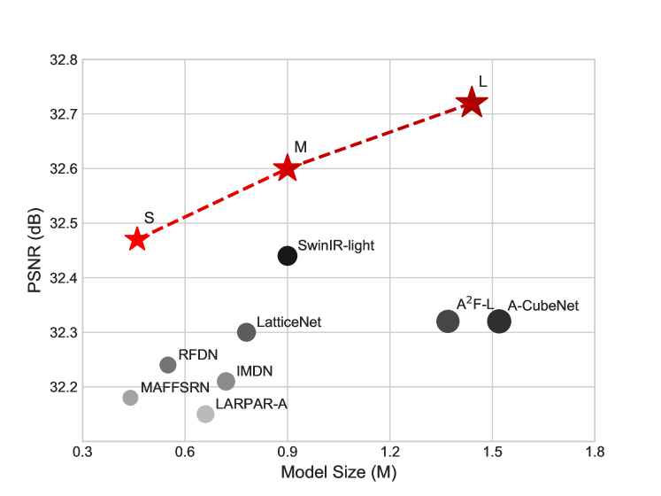
Though CNN-based models have achieved significant improvement compared with traditional methods, they suffer from some inherent problems brought by the local processing principle of convolution kernels. Recent study (Gu and Dong 2021) shows that SR networks with a wide range of involved input pixels could achieve better performance. However, most of the CNN-based models adopt a small convolution kernel (e.g. $3\times 3$) where only a limited range of pixels are aggregated. Alternatively, the self-attention mechanism in Transformer (Dosovitskiy et al. 2020) models can model long-range dependencies of input pixels and several attempts have already made in the task of SISR. In this paper, we also focus on the self-attention mechanism for aggregating pixels in a wide range of input pixels.

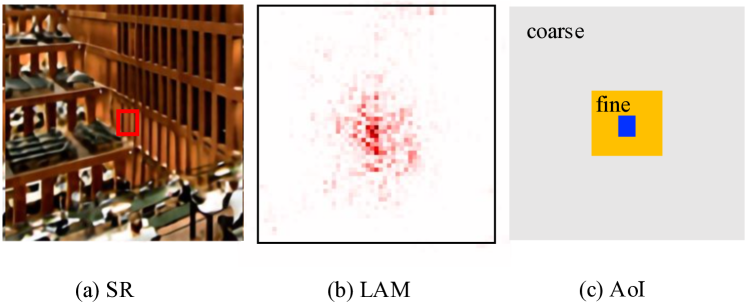
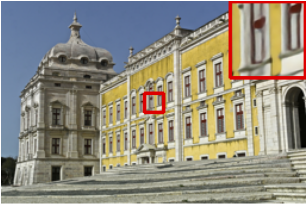
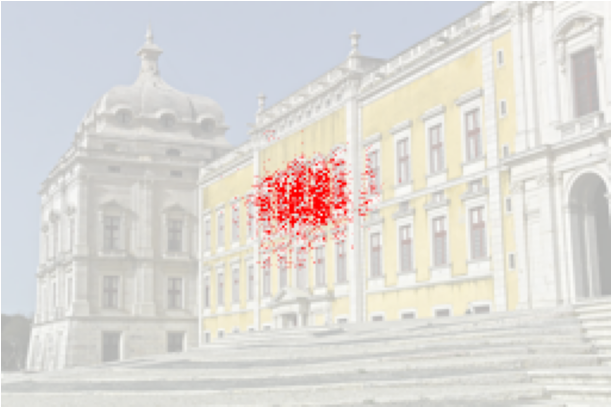
The pioneering vision Transformer (Dosovitskiy et al. 2020) adopts a redundant attention manner, whose computation complexity is quadratic to the image size. The large computation complexity makes it difficult to be applied for high-resolution predictions in SISR task. Some recent proposals apply self-attention within a small spatial region (Chen et al. 2021; Liang et al. 2021; Wang et al. 2021) to alleviate this issue. However, these methods lack direct interaction between distant pixels, which is critical for achieving good performance (Gu and Dong 2021). In (Gu and Dong 2021), a Local Attribution Map (LAM) is proposed to give a deep understanding of SR networks. As shown in Fig. 2b, the LAM map represents the importance of each pixel in the input LR image with respect to the SR of the patch marked with a red box (Fig. 2a). Based on the LAM map, we define a Area of Interest (AoI) map in Fig. 2c. The AoI map presents a hierarchical manner that the most important pixels are located in a fine area (yellow area in Fig. 2c) of a patch and some less important pixels are spread in a coarse area (gray area in Fig. 2c) of the whole image. Further, we use a blue box in Fig. 2c to represent the area with highest interest. In this paper, we use the terms coarse and fine to describe the density of important pixels and the granularity of operations interchangeably. According to this hierarchical partition, we believe that a well-designed SR network should (1) have the ability to focus on processing the finest detail in very local area (e.g., the blue area); (2) be capable of modeling long-range dependencies in a certain area (e.g., the yellow area) to utilize the surrounding context for better reconstruction; (3) have a mechanism to access important pixels in a coarse area (e.g., the gray area) of an input image.

Figure 2: (a) SR result of RNAN (Zhang et al. 2019). (b) Local Attribution Map (LAM) (Gu and Dong 2021). (c) Area of Interest (AoI). The AoI is defined according to the coarse-to-fine hierarchy of important pixels in LAM.

Based on these observations, we propose a novel Hierarchical Pixel Integration (HPI) block that consists of three main parts: a Global Pixel Access (GPA) module, an Intra-Patch Self-Attention (IPSA) module, and a $3\times 3$ convolution. The GPA module is responsible for pixel access in coarse area. Specifically, a similarity map between each pair of image patches is calculated and the most similar patch is selected to conduct cross-attention with current patch. In this way, important pixels in the coarse area can be integrated into current patch efficiently. After fusing pixels from coarse area, we apply the standard self-attention to model long-range dependencies in the fine area of a patch. Finally, a $3\times 3$ convolution is adopted to refine local details in the finest area. Besides, we found in experiments that the vanilla patch division hinders the perceptual quality of recovered images. To tackle this issue, we propose to use a Cascaded Patch Division (CPD) that gradually enlarges the patch window in different blocks.

In summary, our main contributions are as follows:

• We introduce a hierarchical interpretation of the Local Attention Map (LAM) (Gu and Dong 2021) and devise a new attention block for image SR.

• Instead of the vanilla patch division method that fixes the patch size throughout the network, a Cascaded Patch Division (CPD) strategy is applied for better perceptual quality in terms of LPIPS.

• We propose a lightweight Hierarchical Pixel Access Network (HPINet) that outperforms existing lightweight SR methods by a large margin. Most notably, our HPINet achieves results that match state-of-the-art large (around 15M) SR models using less than 1.5M parameters.

RELATED WORK

Deep Neural Networks for SR

Deep neural networks have become the most popular methodology for image SR in the past several years thanks to their great representation power. Since (Dong et al. 2014) first uses three convolution layers to map the low-resolution images to high-resolution images, various CNN-based networks have further enhanced the state-of-the-art performance via better architecture design, such as residual connections (Kim, Lee, and Lee 2016a, b; Liu, Tang, and Wu 2020; Liu et al. 2020; Wang et al. 2018), U-shape architecture (Cheng et al. 2019; Mao, Shen, and Yang 2016; Liu et al. 2018) and attention mechanisms (Hui et al. 2019; Zhang et al. 2018b; Zhao et al. 2020; Niu et al. 2020; Wu et al. 2020).

In addition to improving accuracy, some CNN-based works pursue a lightweight and economical structure. Specifically, IDN (Hui, Wang, and Gao 2018) stacks multiple information distillation blocks to extract more useful information. Each block divides feature maps into two parts. One part is reserved and the other is further enhanced by several convolutions. After that two kinds of features are combined for more abundant information. Based on information distillation block, IMDN (Hui et al. 2019) utilizes information multi-distillation block, which retains and process partial feature maps step-by-step, and aggregates them by contrast-aware channel attention mechanism. Furthermore, RFDN (Liu, Tang, and Wu 2020) applies intensive residual learning to distill more efficient feature representations.

While CNN-based methods have dominated this field for a long time, recent works introduce Transformer (Dosovitskiy et al. 2020) and make impressive progress. IPT (Chen et al. 2021) is one of the first methods use Transformer in image SR. However, IPT contains a massive amount of parameters and requires large-scale datasets for training, which limits its practice in real applications. Modified from Swin Transformer (Liu et al. 2021), SwinIR (Liang et al. 2021) limits the attention region in fixed-size windows and uses shift operation to exchange information through nearby windows. As such, it achieves a better trade-off between PSNR and the number of parameters than prevalent CNN-based models. Despite the success, SwinIR set the window size as $8\times 8$, which is larger than a regular convolution (often $3\times 3$ or $5\times 5$) but much smaller than the conventional Transformer (i.e., the entire image), thereby requiring stacking a great number of blocks to achieve sufficiently large receptive fields. In contrast, our HPINet is able to exploit global context even in the first block, which is beneficial for integrating important pixels with fine detail in the early stage.

Figure 3: Overall network architecture of HPINet. The upsampling operation on skip connection between $I_{LR}$ and $I_{SR}$ is omitted for clarity.

(a)

(b)

(c)

Figure 4: Different strategies of patch division. Areas of different colors represent patches in different network layers. The white point represents the sampled pixel whose blind spot is covered with white shadows. (a) vanilla patch division; (b) shift-based patch division; (c) cascaded patch division (ours).

Method

Network Architecture

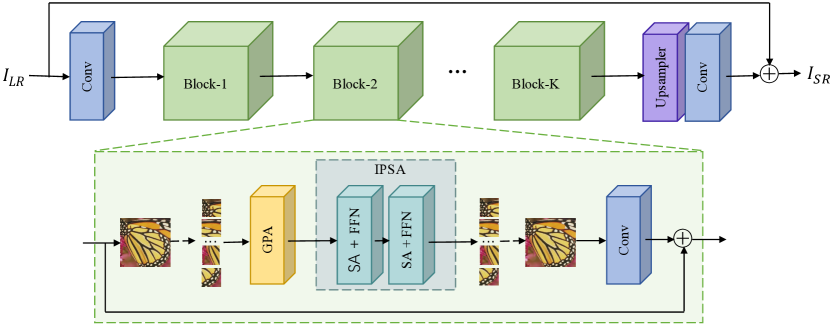
As shown in Fig. 3, the proposed HPINet consists of three components: encoder, Hierarchical Pixel Integration (HPI) block, and decoder. Encoder is a $3\times 3$ convolutional layer which serves to map the input image space to a higher dimensional feature space. Let $I_{\text{LR}}$ and $I_{\text{SR}}$ denote the low resolution input image and the super-resolved image, respectively. We first get shallow feature $x_{0}$ by

$$x_{0}=f_{\text{Encoder}}(I_{\text{LR}}),$$ (1)

where $f_{\text{Encoder}}$ denotes the function of the encoder. Then deeper features are extracted by $K$ sequential HPI blocks. The HPI block consists of five parts: Cascaded Patch Division (CPD), Global Pixel Access (GPA), Intra-Patch Self-Attention (IPSA), Patch Aggregation (PA), and $3\times 3$ Convolution (Conv). The input feature is divided into patches by the CPD module and finally aggregated together via patch aggregation. Formally, in the $i_{\text{th}}$ block, the output feature $x_{i}$ is obtained by

$$x_{i}=x_{i-1}+f_{\text{Conv}}(f_{\text{PA}}(f_{\text{IPSA}}(f_{\text{GPA}}(f_{\text{CPD}}(x_{i-1}))))),$$ (2)

where $f(\cdot)$ denotes the function of each individual component. As with existing works, residual learning is used to assist the training process.

Finally, decoder with pixel-shuffle operations (Shi et al. 2016) is adopted to get the global residual information, which is added to $I_{\text{LR}}$ for restoring the high-resolution output

$$I_{\text{SR}}=I_{\text{LR}}+f_{\text{Decoder}}(x_{K}).$$ (3)

Figure 5: Illustration of Global Pixel Access (GPA) module. * denotes that diagonal elements of the similarity map are set to zero.

Cascaded Patch Division

In order to reduce the computational complexity for lightweight image SR, we split the input feature map into a collection of equal-sized patches and process each patch independently. Specifically, given an input $\mathbf{X}$ of size $H\times W\times C$, we split it into a set of square patches, i.e., $\mathbf{X}=\{\mathbf{X}_{i}\in\mathbb{R}^{P^{2}\times C}\>|\>i=1,\cdots,N\}$, where $P$ is the patch size and $N$ stands for the total number of patches. Each patch must satisfy

$$u\>\%\>P =0\quad\text{or}\quad u=H-P\;$$ (4)

$$v\>\%\>P =0\quad\text{or}\quad v=W-P\;$$ (5)

where $(u,v)$ denotes the coordinate of pixel in the top-left corner. All patches can be processed in parallel, after which the outputs are pasted to their original location in patch aggregation module. It is worthwhile to note that such cropping strategy is adaptive to arbitrary input size, which means no padding pixels are needed.

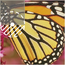
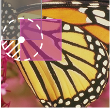
Though this vanilla division greatly reduces computational cost, it limits the receptive field of boundary pixels. Unlike pixels around the center of a patch, border pixels can not directly interact with neighboring pixels that are out of the patch (see Fig. 4a), which may deteriorate the visual quality of reproduced images. In practice, patch overlapping is useful but not effective enough. Other attempts like (Liang et al. 2021) use shift operations to re-divide patches, but there are still pixels that fail to reach their neighbors directly (see Fig. 4b). Inspired by the idea of progressive learning, we just assign different patch size $P$ to different blocks in a cascaded manner. In other words, we enlarge $P$ progressively in the network. As a result, the border pixels of a block could be in the center of later blocks. Therefore, there exist non-persistent boundaries (see Fig. 4c). It also comes with the added bonus that a smaller receptive filed in the shallow layers helps stabilize the training process, while a larger receptive field in deep layers enables smoother pixel integration. Experiments indicate that the Cascaded Patch Division (CPD) strategy is fairly simple yet effective.

Intra-Patch Self-Attention

Before the introduction of our GPA module, we first describe the detail of Intra-Patch Self-Attention (IPSA) for a better understanding. IPSA follows the standard self-attention paradigm (Dosovitskiy et al. 2020), whereas there are two changes. Firstly, IPSA is performed at patch level instead of image level. Secondly, positional embedding is removed because of the introduce of the convolutional layer, which can learn positional relations implicitly and make the network more concise and efficient. IPSA is responsible for modeling long-range dependencies in a patch so that the context information could be fully utilized.

More specifically, for a patch feature $\mathbf{X}\in\mathbb{R}^{P^{2}\times C}$, the query, key and value matrices $\mathbf{Q}\in\mathbb{R}^{P^{2}\times d}$, $\mathbf{K}\in\mathbb{R}^{P^{2}\times d}$, $\mathbf{V}\in\mathbb{R}^{P^{2}\times C}$ are computed as

$$\mathbf{Q}=\mathbf{XW}_{Q},\quad\mathbf{K}=\mathbf{XW}_{K},\quad\mathbf{V}=\mathbf{XW}_{V},$$ (6)

where $\mathbf{W}_{Q}$, $\mathbf{W}_{K}$ and $\mathbf{W}_{V}$ are weight matrices that are shared across patches. By comparing the similarity between $\mathbf{Q}$ and $\mathbf{K}$, we obtain a attention map of size $\mathbb{R}^{P^{2}\times P^{2}}$ and multiply it with $\mathbf{V}$. Overall, the calculation of Self-Attention (SA) can be formulated as

$$SA(\mathbf{X})=\text{softmax}(\mathbf{QK}^{T}/\sqrt{d})\mathbf{V}.$$ (7)

Here $\sqrt{d}$ is used to control the magnitude of $\mathbf{QK}^{T}$ before applying the softmax function.

Similar to the conventional Transformer layer (Dosovitskiy et al. 2020), the Feed Forward Network (FFN) is employed after SA module to further transform features. FFN contains two fully-connected layers, and one GELU non-linearity is applied after the first linear layer. Besides, layer normalization is added before SA module and FFN module, and residual shortcuts after both modules are added as well.

Global Pixel Access

In this part, we aim to integrate important pixels belonging to the coarse area of a LAM map (see Fig. 2). SR Networks with a wider range of effective receptive field have been proven to achieve better performance (Gu and Dong 2021). The problem is how to make the network be capable of modeling global connectivity while maintaining computational efficiency. Since the partition of patch is fixed for a layer, there is no direct connection across patches. A straightforward way is to mix the information of every patch pair exhaustively. However, it is unnecessary and inefficient given the fact that many patches are irrelevant and uninformative. Moreover, redundant interaction may introduce extra noise that hinders the model performance.

Based on these observations, we propose an innovative Global Pixel Access (GPA) module, in which each patch performs adaptive pixel integration with the most correlative counterpart (see Fig. 5). To be specific, firstly, all patches are spatially pooled into one-dimensional tokens. These tokens encode the characteristic of the patches, which are later used for similarity calculation and patch matching. This process can be expressed as

$$\overline{\mathbf{X}}_{i}=\mathop{\arg\max}\limits_{\mathbf{X}_{j}}\;L(\mathbf{X}_{i})^{T}L(\mathbf{X}_{j}),\quad j\neq i,$$ (8)

where $\overline{\mathbf{X}}_{i}$ is the best-matching patch with $X_{i}$, and $L(\cdot)$ is the average pooling function along spatial dimension followed by flatten operation and layer normalization. Since the $argmax$ opration is non-differentiable, we replace it with Gumbel-Softmax opration (Jang, Gu, and Poole 2016) during training so as to make it possible to train end-to-end. After that, pixel information of $\overline{\mathbf{X}}_{i}$ are fused into $\mathbf{X}_{i}$ via Cross-Attention (CA)

$$\mathbf{X}_{i}=\text{CA}(\mathbf{X}_{i},\overline{\mathbf{X}}_{i}).$$ (9)

As illustrated in Fig. 5, CA works in a similar way to the standard self-attention (Dosovitskiy et al. 2020), but the key and value are calculated using $\overline{\mathbf{X}}_{i}$ in Equation (Eq. 6). As a result, GPA can enable global pixel integration while introducing little computational overhead.

Local $3\times 3$ Convolution

The aforementioned GPA and IPSA can integrate information from a wide range of pixels. However, as indicates by the LAM map in Fig. 2b, the most import pixels usually locate in a local area of a patch. Therefore, we need a more local operation to process local detail in a fine-grained manner. We found that a simple $3\times 3$ convolution is efficient and effective for this task due to the local processing principle of convolution kernel.

Experiments

Datasets and Evaluation Metrics

The model is trained with a high-quality dataset DIV2K (Agustsson and Timofte 2017), which is widely used for image SR task. It includes 800 training images together with 100 validation images. Besides, we evaluate our model on five public SR benchmark datasets: Set5 (Bevilacqua et al. 2012), Set14 (Zeyde, Elad, and Protter 2010), B100 (Martin et al. 2001), Urban100 (Huang, Singh, and Ahuja 2015) and Manga109 (Matsui et al. 2017).

We use objective criteria, i.e., peak signal-to-noise ratio (PSNR), structural similarity index (SSIM) to evaluate our model performance. As adopted in the previous work, the two metrics are both calculated on the Y channel after converting to YCbCr space. Besides, we report total number of parameters to compare the complexity of different models.

Implementation Details

Motivated by (Zamir et al. 2021), we adopt progressive learning during training process. The cropped HR image size is initialized as 196$\times$196 and increases to 896$\times$896 epoch by epoch, and batch size is set as 6. Training images are augmented by random flipping and rotation. All models are trained using Adam algorithm with L1 loss. The learning rate is initialized as $3\times 10^{-4}$ and halved per 200 epochs. For the proposed HPINet, the number of blocks is set as 8 and the corresponding patch size is set as $\left\{12,16,20,24,12,16,20,24\right\}$. The whole process is implemented by Pytorch on NVIDIA Tesla V100 GPUs. More specific details will be explained in the respective subsection.

Figure 6: Visual comparison with state-of-the-art lightweight SR methods on Urban100, including IDN (Hui, Wang, and Gao 2018), CARN (Ahn, Kang, and Sohn 2018), IMDN (Hui et al. 2019), A²F-L (Wang et al. 2020), and SwinIR-light (Liang et al. 2021).

Table 1: Quantitative Comparisons of HPINet with Existing Lightweight SR Models on Benchmark Datasets. Our Models are Marked in Bold. Best and Second Best Performance are Highlighted in Red and Blue Colors, Respectively. “Param” Is the Number of Parameters

Scale	Model	Param	Set5 PSNR/SSIM	Set14 PSNR/SSIM	B100 PSNR/SSIM	Urban100 PSNR/SSIM	Manga109 PSNR/SSIM
$\times 2$	FALSR-C	0.41M	37.66/0.9586	33.26/0.9140	31.96/0.8965	31.24/0.9187	-
	DRRN	0.30M	37.74/0.9591	33.23/0.9136	32.05/0.8973	31.23/0.9188	37.92/0.9760
	CARN	1.59M	37.76/0.9590	33.52/0.9166	32.09/0.8978	31.92/0.9256	38.36/0.9765
	FALSR-A	1.02M	37.82/0.9595	33.55/0.9168	32.12/0.8987	31.93/0.9256	-
	IDN	0.55M	37.83/0.9600	33.30/0.9148	32.08/0.8985	31.27/0.9196	38.88/0.9774
	A2F-SD	0.31M	37.91/0.9602	33.45/0.9164	32.08/0.8986	31.79/0.9246	38.52/0.9767
	MAFFSRN	0.40M	37.97/0.9603	33.49/0.9170	32.14/0.8994	31.96/0.9268	-
	PAN	0.26M	38.00/0.9605	33.59/0.9181	32.18/0.8997	32.01/0.9273	38.70/0.9773
	IMDN	0.69M	38.00/0.9605	33.63/0.9177	32.19/0.8999	32.17/0.9283	38.01/0.9749
	LAPAR-A	0.55M	38.01/0.9605	33.62/0.9183	32.19/0.8999	32.10/0.9283	38.67/0.9772
	RFDN	0.53M	38.05/0.9606	33.68/0.9184	32.16/0.8994	32.12/0.9278	38.88/0.9773
	A2F-L	1.36M	38.09/0.9607	33.78/0.9192	32.23/0.9002	32.46/0.9313	38.95/0.9772
	A-CubeNet	1.38M	38.12/0.9609	33.73/0.9191	32.26/0.9007	32.39/0.9308	38.88/0.9776
	LatticeNet	0.76M	38.15/0.9610	33.78/0.9193	32.25/0.9005	32.43/0.9302	-
	SwinIR-light	0.88M	38.14/0.9611	33.86/0.9206	32.31/0.9012	32.76/0.9340	39.12/0.9783
	HPINet (Ours)	0.78M	38.12/0.9605	33.94/0.9209	32.31/0.9013	32.85/0.9346	39.08/0.9771
$\times 3$	DRRN	0.30M	34.03/0.9244	29.96/0.8349	28.95/0.8004	27.53/0.8378	32.74/0.9390
	IDN	0.55M	34.11/0.9253	29.99/0.8354	28.95/0.8013	27.42/0.8359	32.71/0.9381
	A2F-SD	0.32M	34.23/0.9259	30.22/0.8395	29.01/0.8028	27.91/0.8465	33.29/0.9424
	CARN	1.59M	34.29/0.9255	30.29/0.8407	29.06/0.8034	28.06/0.8493	33.50/0.9440
	MAFFSRN	0.42M	34.32/0.9269	30.35/0.8429	29.09/0.8052	28.13/0.8521	-
	IMDN	0.70M	34.36/0.9270	30.32/0.8417	29.09/0.8046	28.17/0.8519	33.61/0.9445
	LAPAR-A	0.59M	34.36/0.9267	30.34/0.8421	29.11/0.8054	28.15/0.8523	33.51/0.9441
	PAN	0.26M	34.40/0.9272	30.36/0.8422	29.11/0.8049	28.11/0.8511+	33.61/0.9448
	RFDN	0.54M	34.41/0.9273	30.34/0.8420	29.09/0.8050	28.21/0.8525	33.67/0.9449
	LatticeNet	0.77M	34.53/0.9281	30.39/0.8424	29.15/0.8059	28.33/0.8538	-
	A-CubeNet	1.56M	34.53/0.9281	30.45/0.8441	29.17/0.8068	28.38/0.8568	33.90/0.9466
	A2F-L	1.37M	34.54/0.9283	30.41/0.8436	29.14/0.8062	28.40/0.8574	33.83/0.9463
	SwinIR-light	0.89M	34.62/0.9289	30.54/0.8463	29.20/0.8082	28.66/0.8624	33.98/0.9478
	HPINet (Ours)	0.92M	34.70/0.9289	30.63/0.8480	29.26/0.8104	28.93/0.8675	34.31/0.9487
$\times 4$	DRRN	0.30M	31.68/0.8888	28.21/0.7720	27.38/0.7284	25.44/0.7638	29.46/0.8960
	IDN	0.55M	31.82/0.8903	28.25/0.7730	27.41/0.7297	25.41/0.7632	29.41/0.8942
	A2F-SD	0.32M	32.06/0.8928	28.47/0.7790	27.48/0.7373	25.80/0.7767	30.16/0.9038
	CARN	1.59M	32.13/0.8937	28.60/0.7806	27.58/0.7349	26.07/0.7837	30.47/0.9084
	PAN	0.27M	32.13/0.8948	28.61/0.7822	27.59/0.7363	26.11/0.7854	30.51/0.9095
	LAPAR-A	0.66M	32.15/0.8944	28.61/0.7818	27.61/0.7366	26.14/0.7871	30.42/0.9074
	MAFFSRN	0.44M	32.18/0.8948	28.58/0.7812	27.57/0.7361	26.04/0.7848	-
	IMDN	0.72M	32.21/0.8948	28.58/0.7811	27.56/0.7353	26.04/0.7838	30.45/0.9075
	RFDN	0.55M	32.24/0.8952	28.61/0.7819	27.57/0.7360	26.11/0.7858	30.58/0.9089
	LatticeNet	0.78M	32.30/0.8962	28.68/0.7830	27.62/0.7367	26.25/0.7873	-
	A2F-L	1.37M	32.32/0.8964	28.67/0.7839	27.62/0.7379	26.32/0.7931	30.72/0.9115
	A-CubeNet	1.52M	32.32/0.8969	28.72/0.7847	27.65/0.7382	26.27/0.7913	30.81/0.9114
	SwinIR-light	0.90M	32.44/0.8976	28.77/0.7858	27.69/0.7406	26.47/0.7980	30.92/0.9151
	HPINet (Ours)	0.90M	32.60/0.8986	28.87/0.7874	27.73/0.7419	26.71/0.8043	31.19/0.9161

Table 2: Ablation Study on the Cascaded Patch Division (CPD) and Global Pixel Access (GPA). Metrics (PSNR$\uparrow$/SSIM$\uparrow$/LPIPS$\downarrow$) Are Calculated on Benchmark Datasets with a Scale Factor of 4, Where “$\uparrow$” Indicates Higher Is Better and “$\downarrow$” Means Lower Is Better. Best and Second Best Result Are in Red and Blue Colors, Respectively

Model	CPD	GPA	Param	Multi-Adds	Set5 PSNR$\uparrow$/SSIM$\uparrow$/LPIPS$\downarrow$	Set14 PSNR$\uparrow$/SSIM$\uparrow$/LPIPS$\downarrow$	B100 PSNR$\uparrow$/SSIM$\uparrow$/LPIPS$\downarrow$	Urban100 PSNR$\uparrow$/SSIM$\uparrow$/LPIPS$\downarrow$	Manga109 PSNR$\uparrow$/SSIM$\uparrow$/LPIPS$\downarrow$
①	✗	✗	895K	121.7G	32.46/0.8974/0.1760	28.83/0.7859/0.2844	27.70/0.7400/0.3444	26.57/0.7995/0.2125	31.00/0.9144/0.1149
②	✓	✗	895K	123.9G	32.50/0.8979/0.1735	28.83/0.7869/0.2817	27.71/0.7416/0.3421	26.63/0.8018/0.2094	31.04/0.9151/0.1139
③	✗	✓	896K	121.8G	32.50/0.8977/0.1757	28.86/0.7865/0.2868	27.72/0.7408/0.3476	26.63/0.8006/0.2163	31.08/0.9150/0.1155
④	✓	✓	896K	124.0G	32.60/0.8986/0.1729	28.87/0.7874/0.2826	27.73/0.7419/0.3433	26.71/0.8043/0.2100	31.19/0.9161/0.1127

Comparisons with the state-of-the-arts

We compare the proposed HPINet with commonly used lightweight SR models for upscaling factor $\times$2, $\times$3, and $\times$4, including FALSR (Chu et al. 2021), DRRN (Tai, Yang, and Liu 2017), A²F (Wang et al. 2020), MAFFSRN (Muqeet et al. 2020), PAN (Zhao et al. 2020), IDN (Hui, Wang, and Gao 2018), IMDN (Hui et al. 2019), LAPAR (Li et al. 2020), RFDN (Liu, Tang, and Wu 2020), SwinIR (Liang et al. 2021), CARN (Ahn, Kang, and Sohn 2018), LatticeNet (Luo et al. 2020) and A-CubeNet (Hang et al. 2020). The comparison results are classified into several groups according to the upscaling factor.

Quantitative Comparison

Table 1 shows quantitative results in terms of PSNR and SSIM on five benchmark datasets obtained by different algorithms. As shown in Table 1, our HPINet achieves the best performance for $\times 3$ and $\times 4$ SR. For $\times 2$ SR, we also achieve superior results than the state-of-the-art SwinIR-light model on Set14, B100 and Urban100 datasets with 0.1M fewer parameters. It is notable that our HPINet outperforms SwinIR-light by a maximum PSNR of 0.27dB, which is a significant improvement for image SR.

Qualitative Comparison

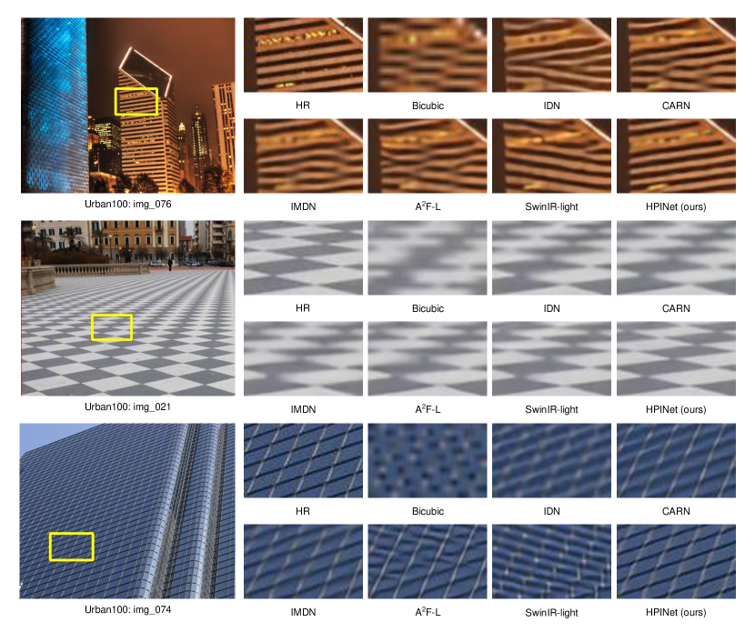
We further show visual examples of different methods under scaling factor $\times 4$. As shown in Fig. 6, our HPINet can recover more details than IDN, CARN, IMDN, A²F-L and SwinIR-light, which indicates the superiority of our method.

(a) w/ GPA

(b) w/o GPA

Figure 7: LAM (Gu and Dong 2021) comparison between the full HPINet (w/ GPA) and the variant without GPA (w/o GPA) for $\times 4$ SR. The first row shows input along with the predicted result, and the second row shows the effective receptive field. Zoom in for better view.

Figure 8: Visualization of patch pairs that best match. Patches with different size come from different blocks in the network.

Ablation Analysis

In this section, we conduct ablation experiments to study the effect of Cascaded Patch Division (CPD) and Global Pixel Access (GPA). Evaluations are performed on Set5 (Bevilacqua et al. 2012), set14 (Zeyde, Elad, and Protter 2010), B100 (Martin et al. 2001), Urban100 (Huang, Singh, and Ahuja 2015) and Manga109 (Matsui et al. 2017) datasets. Besides PSNR and SSIM, LPIPS (Zhang et al. 2018a) is adopted to evaluate the perceptual quality of recovered images as well. It can provide better judgment of image quality when two models have similar performances in terms of PSNR and SSIM. We also adopt multiply-accumulate operations (Multi-Adds) on a $1280\times 720$ query image to evaluate computational complexity.

We start with a naive baseline by removing both components (model ①). Then we add CPD (model ②) and GPA (model ③) to the baseline, respectively. At last, both components are employed to compose our final version of method (model ④). The results are reported in Table 2.

Effectiveness of CPD

To show the effect of CPD, we instantiate model ③ where all blocks share the same patch size for comparison. The patch size is fixed as 18 to maintain similar Multi-Adds. As shown in Table 2, model ④ improves the performance of model ③ on all metrics. The same phenomena can also be observed by comparing model ② and model ①, where the LPIPS gets substantially improvement by adding CPD. It is notable that the model with CPD turns out to achieve better SSIM and LPIPS, even when its PSNR results are indistinguishable. These results validate that CPD can provide not only higher image similarity but also better perceptual quality.

Effectiveness of GPA

A core feature of our HPINet is its ability to access global pixel effectively. To highlight the contribution of global modeling, we drop GPA in model ② for comparison, meanwhile expanding IPSA modules to keep similar parameter budget. Recall that IPSA only integrates pixels within a patch. Comparing model ② and model ④, we can observe that with the help of GPA, the PSNR and SSIM get consistent improvements on all five datasets. Specifically, the PSNR increases by a maximum of 0.15dB, which is a notable boost in lightweight image SR. Interestingly, the LPIPS on several benchmark datasets gets worse after adding GPA to the baseline model, and we guess it is caused by the introduction of noisy pixels. This problem can be greatly reduced by using the proposed CPD module, which can be observed by comparing model ③ with model ④.

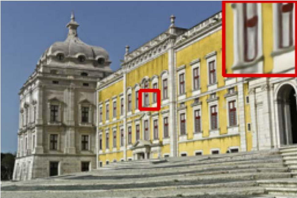
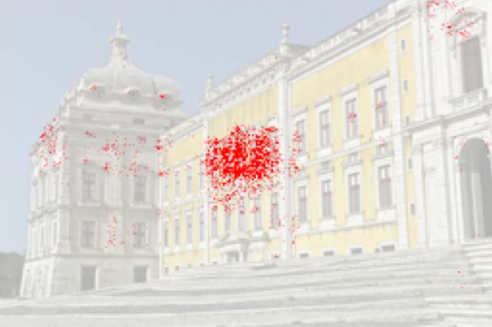
To better understand the main reason of the improvement brought by GPA, we utilize LAM (Gu and Dong 2021) to visualize the effective receptive field of a input patch. As shown in Fig. 7, the patch benefits from a global range of useful pixels by using GPA. In Fig. 8, we further present examples of patch pairs that matched and selected by GPA in different blocks. It can be found that each patch pair share some visual similarities, which could facilitate restoring more details. All results indicate the effectiveness of the proposed GPA in improving PSNR and SSIM performances.

Table 3: Parameter, Running Time and PSNR Comparison for Scale Factor $\times 4$

Model	Param(M)	Set5 PSNR(dB)/Time(ms)	Set14 PSNR(dB)/Time(ms)	B100 PSNR(dB)/Time(ms)	Urban100 PSNR(dB)/Time(ms)	Manga109 PSNR(dB)/Time(ms)
RCAN (Zhang et al. 2018b)	15.6	32.63/56	28.87/65	27.77/61	26.82/119	31.22/157
SAN (Dai et al. 2019)	15.9	32.64/68	28.92/127	27.78/58	26.79/997	31.18/1771
SwinIR (Liang et al. 2021)	11.9	32.72/65	28.94/117	27.83/75	27.07/401	31.67/521
SwinIR-light (Liang et al. 2021)	0.90	32.44/47	28.77/59	27.69/48	26.47/158	30.92/198
HPINet-L	1.44	32.72/39	28.97/51	27.79/40	26.95/144	31.47/220
HPINet-M	0.90	32.60/38	28.87/49	27.73/39	26.71/137	31.19/194
HPINet-S	0.46	32.47/34	28.80/48	27.69/36	26.59/131	30.92/160

Table 4: Ablation Study on IPSA and $3\times 3$ Conv. The PSNR Results on Five Benchmark Datasets Are Included

Model	Set5	Set14	B100	Urban100	Manga109
w/o IPSA	32.26	28.66	27.60	26.30	30.66
w/o $3\times 3$ conv	32.09	28.63	27.57	26.17	30.55
HPINet (full)	32.60	28.87	27.73	26.71	31.19

Effectiveness of IPSA

The IPSA module can model long-range dependencies in a patch. To prove the effectiveness of this module, we remove IPSA from all the attention blocks and replace it with depth-wise convolutions to maintain a similar number of parameters. As shown in the first row of Table 4, the model “w/o IPSA” behaves much worse than the full HPINet model, which indicates the importance of IPSA in improving the SR performance. Compared with conventional convolutions, the IPSA can benefit from a wider range of surrounding pixels and thus achieves much higher PSNR values.

Effectiveness of $3\times 3$ Conv

The HPI attention block is designed in a hierarchical manner that the tail $3\times 3$ convolution is responsible for processing the finest local details. As shown in the second row of Table 4, the model “w/o $3\times 3$ Conv” achieves much lower PSNR values than the full model, which meets the expectation. It indicates convolution plays a basic role even in Transformer-like models, which is in line with conclusions from other vision task (Wu et al. 2021; Guo et al. 2022; Yuan et al. 2021). It is worth emphasizing that convolution is indispensable but not competitive enough. For example, with the equipment of IPSA and GPA, our proposed HPINet surpasses the pure convolution-based model RCAN (Zhang et al. 2018b) in all datasets with $10\times$ fewer parameters (See Table 3). Thus it is hard to replace IPSA and GPA with convolution while maintaining similar performance. Together with the aforementioned results, the observation proves effectiveness of our hierarchical design.

Model Size and and Running Time Analyses

To demonstrate the effectiveness and efficiency of HPINet, we design three variants with different model size (S/M/L) and evaluate their PSNR results and speed on five datasets. For simplicity, All variants only differ in number of channels.

Model Size

The curve of PSNR v.s. model size is depicted in Fig. 1 and the detailed complexity of the three models are included in Table 3. We compare our HPINet with other lightweight SR models of various sizes, including MAFFSRN (Muqeet et al. 2020), RFDN (Liu, Tang, and Wu 2020), LAPAR-A (Li et al. 2020), IMDN (Hui et al. 2019), LatticeNet (Luo et al. 2020), SwinIR-light (Liang et al. 2021), A²F-L (Wang et al. 2020) and A-cubeNet (Hang et al. 2020). Our HPINet-S/M/L achieves much higher PSNR than all other lightweight models at each size. Specially, HPINet-L outperforms RCAN (15.6M) and SAN (15.9M) with less than 1.5M parameters.

Running Time

To reduce the accidental error, we run each model for 10 times on one GPU and calculate the average time as the final running time. We also compare them with other advanced models, including RCAN (Zhang et al. 2018b), SAN (Dai et al. 2019) and SwinIR (Liang et al. 2021). RCAN (Zhang et al. 2018b) is a classic CNN-based model and SAN (Dai et al. 2019) is a often-cited model equipped with non-local modules. SwinIR (Liang et al. 2021) is a state-of-the-art Transformer-based model. According to Table 3, several observations can be summarized as follows: (1) With the same (i.e., HPINet-M) or fewer parameters (i.e., HPINet-S), our model runs faster than SwinIR-light whiling maintaining higher PSNR values. (2) When using a slightly larger model, i.e., HPINet-L, we can even achieve superior or comparable PSNR values with very large models including RCAN, SAN and SiwnIR. (3) Our HPINet runs faster than all other models on Set5, Set14 and B100 datasets. As the image resolution increases on Urban100 and Manga109 datasets, HPINet is slightly slower than RCAN but much faster than SAN and SwinIR. Overall, the proposed HPINet has a better trade-off between model complexity and PSNR.

Conclusion

In this paper, we proposed a lightweight single-image super-resolution network called HPINet which sequentially stacks a series of Hierarchical Pixel Integration (HPI) blocks. The HPI block is designed according to the hierarchical interpretation of a LAM map. Specifically, each block consists of three main components: a Global Pixel Access (GPA) module, an Intra-Patch Self-Attention (IPSA) module and a $3\times 3$ convolutional layer. They are responsible for processing input images from coarse to fine. Besides, a Cascaded Patch Division (CPD) strategy is also proposed for better perceptual quality. Benefiting from these components, HPINet can effectively capture the global, long-range and local relations in an efficient manner. Quantitative and qualitative experimental results demonstrate the superior performance of HPINet over previous state-of-the-art SR models on benchmark datasets. In the future, we will try to improve the perceptual quality of GPA and investigate the potential of HPINet in other low-level tasks.

References

- Agustsson and Timofte (2017) Agustsson, E.; and Timofte, R. 2017. Ntire 2017 challenge on single image super-resolution: Dataset and study. In Proceedings of the IEEE conference on computer vision and pattern recognition workshops, 126–135.
- Ahn, Kang, and Sohn (2018) Ahn, N.; Kang, B.; and Sohn, K.-A. 2018. Fast, accurate, and lightweight super-resolution with cascading residual network. In Proceedings of the European conference on computer vision (ECCV), 252–268.
- Bevilacqua et al. (2012) Bevilacqua, M.; Roumy, A.; Guillemot, C.; and Morel, M.-L. A. 2012. Low-Complexity Single-Image Super-Resolution based on Nonnegative Neighbor Embedding. In British Machine Vision Conference (BMVC), 1–10.
- Chen et al. (2021) Chen, H.; Wang, Y.; Guo, T.; Xu, C.; Deng, Y.; Liu, Z.; Ma, S.; Xu, C.; Xu, C.; and Gao, W. 2021. Pre-trained image processing transformer. In Proceedings of the IEEE/CVF Conference on Computer Vision and Pattern Recognition, 12299–12310.
- Cheng et al. (2019) Cheng, G.; Matsune, A.; Li, Q.; Zhu, L.; Zang, H.; and Zhan, S. 2019. Encoder-decoder residual network for real super-resolution. In Proceedings of the IEEE/CVF Conference on Computer Vision and Pattern Recognition Workshops, 0–0.
- Chu et al. (2021) Chu, X.; Zhang, B.; Ma, H.; Xu, R.; and Li, Q. 2021. Fast, accurate and lightweight super-resolution with neural architecture search. In 2020 25th International Conference on Pattern Recognition (ICPR), 59–64.
- Dai et al. (2019) Dai, T.; Cai, J.; Zhang, Y.; Xia, S.-T.; and Zhang, L. 2019. Second-order attention network for single image super-resolution. In Proceedings of the IEEE/CVF conference on computer vision and pattern recognition, 11065–11074.
- Dong et al. (2014) Dong, C.; Loy, C. C.; He, K.; and Tang, X. 2014. Learning a deep convolutional network for image super-resolution. In European conference on computer vision, 184–199.
- Dong, Loy, and Tang (2016) Dong, C.; Loy, C. C.; and Tang, X. 2016. Accelerating the super-resolution convolutional neural network. In European conference on computer vision, 391–407.
- Dosovitskiy et al. (2020) Dosovitskiy, A.; Beyer, L.; Kolesnikov, A.; Weissenborn, D.; Zhai, X.; Unterthiner, T.; Dehghani, M.; Minderer, M.; Heigold, G.; Gelly, S.; et al. 2020. An image is worth 16x16 words: Transformers for image recognition at scale. arXiv preprint arXiv:2010.11929.
- Gu and Dong (2021) Gu, J.; and Dong, C. 2021. Interpreting super-resolution networks with local attribution maps. In Proceedings of the IEEE/CVF Conference on Computer Vision and Pattern Recognition, 9199–9208.
- Guo et al. (2022) Guo, J.; Han, K.; Wu, H.; Tang, Y.; Chen, X.; Wang, Y.; and Xu, C. 2022. Cmt: Convolutional neural networks meet vision transformers. In Proceedings of the IEEE/CVF Conference on Computer Vision and Pattern Recognition, 12175–12185.
- Hang et al. (2020) Hang, Y.; Liao, Q.; Yang, W.; Chen, Y.; and Zhou, J. 2020. Attention cube network for image restoration. In Proceedings of the 28th ACM International Conference on Multimedia, 2562–2570.
- Huang, Singh, and Ahuja (2015) Huang, J.-B.; Singh, A.; and Ahuja, N. 2015. Single image super-resolution from transformed self-exemplars. In Proceedings of the IEEE conference on computer vision and pattern recognition, 5197–5206.
- Hui et al. (2019) Hui, Z.; Gao, X.; Yang, Y.; and Wang, X. 2019. Lightweight image super-resolution with information multi-distillation network. In Proceedings of the 27th acm international conference on multimedia, 2024–2032.
- Hui, Wang, and Gao (2018) Hui, Z.; Wang, X.; and Gao, X. 2018. Fast and accurate single image super-resolution via information distillation network. In Proceedings of the IEEE conference on computer vision and pattern recognition, 723–731.
- Jang, Gu, and Poole (2016) Jang, E.; Gu, S.; and Poole, B. 2016. Categorical reparameterization with gumbel-softmax. arXiv preprint arXiv:1611.01144.
- Kim, Lee, and Lee (2016a) Kim, J.; Lee, J. K.; and Lee, K. M. 2016a. Accurate image super-resolution using very deep convolutional networks. In Proceedings of the IEEE conference on computer vision and pattern recognition, 1646–1654.
- Kim, Lee, and Lee (2016b) Kim, J.; Lee, J. K.; and Lee, K. M. 2016b. Deeply-recursive convolutional network for image super-resolution. In Proceedings of the IEEE conference on computer vision and pattern recognition, 1637–1645.
- Li et al. (2020) Li, W.; Zhou, K.; Qi, L.; Jiang, N.; Lu, J.; and Jia, J. 2020. Lapar: Linearly-assembled pixel-adaptive regression network for single image super-resolution and beyond. Advances in Neural Information Processing Systems, 33: 20343–20355.
- Li et al. (2019) Li, Z.; Yang, J.; Liu, Z.; Yang, X.; Jeon, G.; and Wu, W. 2019. Feedback network for image super-resolution. In Proceedings of the IEEE/CVF conference on computer vision and pattern recognition, 3867–3876.
- Liang et al. (2021) Liang, J.; Cao, J.; Sun, G.; Zhang, K.; Van Gool, L.; and Timofte, R. 2021. Swinir: Image restoration using swin transformer. In Proceedings of the IEEE/CVF International Conference on Computer Vision, 1833–1844.
- Lim et al. (2017) Lim, B.; Son, S.; Kim, H.; Nah, S.; and Mu Lee, K. 2017. Enhanced deep residual networks for single image super-resolution. In Proceedings of the IEEE conference on computer vision and pattern recognition workshops, 136–144.
- Liu, Tang, and Wu (2020) Liu, J.; Tang, J.; and Wu, G. 2020. Residual feature distillation network for lightweight image super-resolution. In European Conference on Computer Vision, 41–55.
- Liu et al. (2020) Liu, J.; Zhang, W.; Tang, Y.; Tang, J.; and Wu, G. 2020. Residual feature aggregation network for image super-resolution. In Proceedings of the IEEE/CVF conference on computer vision and pattern recognition, 2359–2368.
- Liu et al. (2018) Liu, P.; Zhang, H.; Zhang, K.; Lin, L.; and Zuo, W. 2018. Multi-level wavelet-CNN for image restoration. In Proceedings of the IEEE conference on computer vision and pattern recognition workshops, 773–782.
- Liu et al. (2021) Liu, Z.; Lin, Y.; Cao, Y.; Hu, H.; Wei, Y.; Zhang, Z.; Lin, S.; and Guo, B. 2021. Swin transformer: Hierarchical vision transformer using shifted windows. In Proceedings of the IEEE/CVF International Conference on Computer Vision, 10012–10022.
- Luo et al. (2020) Luo, X.; Xie, Y.; Zhang, Y.; Qu, Y.; Li, C.; and Fu, Y. 2020. Latticenet: Towards lightweight image super-resolution with lattice block. In European Conference on Computer Vision, 272–289. Springer.
- Mao, Shen, and Yang (2016) Mao, X.; Shen, C.; and Yang, Y.-B. 2016. Image restoration using very deep convolutional encoder-decoder networks with symmetric skip connections. Advances in neural information processing systems, 29: 2802–2810.
- Martin et al. (2001) Martin, D.; Fowlkes, C.; Tal, D.; and Malik, J. 2001. A database of human segmented natural images and its application to evaluating segmentation algorithms and measuring ecological statistics. In Proceedings Eighth IEEE International Conference on Computer Vision. ICCV 2001, volume 2, 416–425.
- Matsui et al. (2017) Matsui, Y.; Ito, K.; Aramaki, Y.; Fujimoto, A.; Ogawa, T.; Yamasaki, T.; and Aizawa, K. 2017. Sketch-based manga retrieval using manga109 dataset. Multimedia Tools and Applications, 76(20): 21811–21838.
- Muqeet et al. (2020) Muqeet, A.; Hwang, J.; Yang, S.; Kang, J.; Kim, Y.; and Bae, S.-H. 2020. Multi-attention based ultra lightweight image super-resolution. In European Conference on Computer Vision, 103–118.
- Niu et al. (2020) Niu, B.; Wen, W.; Ren, W.; Zhang, X.; Yang, L.; Wang, S.; Zhang, K.; Cao, X.; and Shen, H. 2020. Single image super-resolution via a holistic attention network. In European conference on computer vision, 191–207.
- Shi et al. (2016) Shi, W.; Caballero, J.; Huszár, F.; Totz, J.; Aitken, A. P.; Bishop, R.; Rueckert, D.; and Wang, Z. 2016. Real-time single image and video super-resolution using an efficient sub-pixel convolutional neural network. In Proceedings of the IEEE conference on computer vision and pattern recognition, 1874–1883.
- Tai, Yang, and Liu (2017) Tai, Y.; Yang, J.; and Liu, X. 2017. Image super-resolution via deep recursive residual network. In Proceedings of the IEEE conference on computer vision and pattern recognition, 3147–3155.
- Tai et al. (2017) Tai, Y.; Yang, J.; Liu, X.; and Xu, C. 2017. Memnet: A persistent memory network for image restoration. In Proceedings of the IEEE international conference on computer vision, 4539–4547.
- Wang et al. (2020) Wang, X.; Wang, Q.; Zhao, Y.; Yan, J.; Fan, L.; and Chen, L. 2020. Lightweight single-image super-resolution network with attentive auxiliary feature learning. In Proceedings of the Asian conference on computer vision, volume 12623, 268–285.
- Wang et al. (2018) Wang, X.; Yu, K.; Wu, S.; Gu, J.; Liu, Y.; Dong, C.; Qiao, Y.; and Change Loy, C. 2018. Esrgan: Enhanced super-resolution generative adversarial networks. In Proceedings of the European conference on computer vision (ECCV) workshops, 0–0.
- Wang et al. (2021) Wang, Z.; Cun, X.; Bao, J.; and Liu, J. 2021. Uformer: A general u-shaped transformer for image restoration. arXiv preprint arXiv:2106.03106.
- Wu et al. (2021) Wu, H.; Xiao, B.; Codella, N.; Liu, M.; Dai, X.; Yuan, L.; and Zhang, L. 2021. Cvt: Introducing convolutions to vision transformers. In Proceedings of the IEEE/CVF International Conference on Computer Vision, 22–31.
- Wu et al. (2020) Wu, H.; Zou, Z.; Gui, J.; Zeng, W.-J.; Ye, J.; Zhang, J.; Liu, H.; and Wei, Z. 2020. Multi-grained attention networks for single image super-resolution. IEEE Transactions on Circuits and Systems for Video Technology, 31(2): 512–522.
- Yuan et al. (2021) Yuan, K.; Guo, S.; Liu, Z.; Zhou, A.; Yu, F.; and Wu, W. 2021. Incorporating convolution designs into visual transformers. In Proceedings of the IEEE/CVF International Conference on Computer Vision, 579–588.
- Zamir et al. (2021) Zamir, S. W.; Arora, A.; Khan, S.; Hayat, M.; Khan, F. S.; and Yang, M.-H. 2021. Restormer: Efficient Transformer for High-Resolution Image Restoration. arXiv preprint arXiv:2111.09881.
- Zeyde, Elad, and Protter (2010) Zeyde, R.; Elad, M.; and Protter, M. 2010. On single image scale-up using sparse-representations. In International conference on curves and surfaces, 711–730.
- Zhang, Zuo, and Zhang (2018) Zhang, K.; Zuo, W.; and Zhang, L. 2018. Learning a single convolutional super-resolution network for multiple degradations. In Proceedings of the IEEE conference on computer vision and pattern recognition, 3262–3271.
- Zhang et al. (2018a) Zhang, R.; Isola, P.; Efros, A. A.; Shechtman, E.; and Wang, O. 2018a. The unreasonable effectiveness of deep features as a perceptual metric. In Proceedings of the IEEE conference on computer vision and pattern recognition, 586–595.
- Zhang, Zeng, and Zhang (2021) Zhang, X.; Zeng, H.; and Zhang, L. 2021. Edge-oriented convolution block for real-time super resolution on mobile devices. In Proceedings of the 29th ACM International Conference on Multimedia, 4034–4043.
- Zhang et al. (2018b) Zhang, Y.; Li, K.; Li, K.; Wang, L.; Zhong, B.; and Fu, Y. 2018b. Image super-resolution using very deep residual channel attention networks. In Proceedings of the European conference on computer vision (ECCV), 286–301.
- Zhang et al. (2019) Zhang, Y.; Li, K.; Li, K.; Zhong, B.; and Fu, Y. 2019. Residual non-local attention networks for image restoration. arXiv preprint arXiv:1903.10082.
- Zhang et al. (2018c) Zhang, Y.; Tian, Y.; Kong, Y.; Zhong, B.; and Fu, Y. 2018c. Residual dense network for image super-resolution. In Proceedings of the IEEE conference on computer vision and pattern recognition, 2472–2481.
- Zhao et al. (2020) Zhao, H.; Kong, X.; He, J.; Qiao, Y.; and Dong, C. 2020. Efficient image super-resolution using pixel attention. In European Conference on Computer Vision, 56–72.