GeoUDF: Surface Reconstruction from 3D Point Clouds via Geometry-guided Distance Representation

Abstract

We present a learning-based method, namely GeoUDF, to tackle the long-standing and challenging problem of reconstructing a discrete surface from a sparse point cloud. To be specific, we propose a geometry-guided learning method for UDF and its gradient estimation that explicitly formulates the unsigned distance of a query point as the learnable affine averaging of its distances to the tangent planes of neighboring points on the surface. Besides, we model the local geometric structure of the input point clouds by explicitly learning a quadratic polynomial for each point. This not only facilitates upsampling the input sparse point cloud but also naturally induces unoriented normal, which further augments UDF estimation. Finally, to extract triangle meshes from the predicted UDF we propose a customized edge-based marching cube module. We conduct extensive experiments and ablation studies to demonstrate the significant advantages of our method over state-of-the-art methods in terms of reconstruction accuracy, efficiency, and generality. The source code is publicly available at https://github.com/rsy6318/GeoUDF.

1 Introduction

Surface reconstruction from point clouds is a fundamental and challenging problem in 3D vision, graphics and robotics [17, 26, 9]. Traditional approaches, such as Poisson surface reconstruction [18], compute an occupancy or signed distance field (SDF) by solving Poisson’s equation, resulting in a sparse line system. Then they utilize the Marching Cubes (MC) [22] algorithm to extract iso-surfaces as the reconstructed meshes. These methods are computationally efficient, scalable, resilient to noise and tolerant to registration artifacts. However, they work only for oriented point samples. Recent developments in deep learning have demonstrated that implicit fields, such as binary occupancy fields (BOFs) and signed distance fields (SDFs), can be learned directly from raw point clouds, making them a promising tool for reconstructing surfaces from unoriented point samples.

Although BOFs and SDFS are effective at reconstructing watertight and manifold surfaces, they have limitations when it comes to representing more general types of surfaces, such as those with open boundaries or interior structures. In contrast, the unsigned distance field (UDF) is more powerful in terms of representation ability, and can overcome the above-mentioned limitations of BOFs and SDFs. The existing deep UDF-based methods, such as [11, 38, 16], employ neural networks to regress UDFs from input point clouds. Due to their reliance on the training data, these methods have limited generalizability and cannot deal with unseen objects well. Another technical challenge diminishing UDFs’ practical usage is that one cannot use the conventional MC to extract iso-surfaces directly because UDFs do not have zero-crossings and thus do not provide the required sign-change information of inside or outside. Some methods [16, 40] locally convert a UDF to an SDF in a cubic cell and then apply MC to extract the surface. However, they often fail at corners or edges. Recently, GIFS [38] modifies MC by predicting whether the surface interacts with each cube edge via a neural network.

In this paper, we propose GeoUDF, a new learning-based framework reconstructing the underlying surface of a sparse point cloud. We particularly aim at addressing two fundamental issues of UDFs, namely, (1) how to predict an accurate UDF and its gradients for arbitrary 3D inputs? and (2) how to extract triangle meshes, given a UDF? More importantly, the constructed methods should be well generalized to unseen data. To solve the first issue, we propose a geometry-guided learning module, adaptively approximating the UDF and its gradient of a point cloud by leveraging its local geometry in a decoupled manner. As for the second issue, we propose an edge-based MC algorithm, extracting triangle mesh from any UDF according to the intersection relationship between the surface and the connections of any two vertices of the cubes. In addition, we propose to enhance input point cloud quality by explicitly and concisely modeling its local geometry structure, which is beneficial for surface reconstruction. The elegant formulations distinguish our GeoUDF from existing methods, making it more lightweight, efficient, and accurate and better generalizability. Besides, the proposed modules contained in GeoUDF can be independently used as a general method in its own right. Extensive experiments on various datasets show the significant superiority of our method over state-of-the-art methods.

In summary, the main contributions of this paper are three-fold:

• novel accurate, compact, efficient, and explainable learning-based UDF and its gradient estimation methods that are decoupled;

• a concise yet effective learning-based point cloud upsampling and representation method; and

• a general method for extracting triangle meshes from any unsigned distance field.

2 Related Work

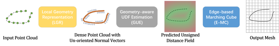
Figure 1: The pipeline of GeoUDF, a lightweight, explainable, and efficient learning-based surface reconstruction framework that produces 3D meshes with high accuracy and strong generalizability.

Learning Implicit Surface Representation. With the development of deep learning, many advances have been made in the implicit representation of 3D shapes in recent years. For example, Binary Occupancy Field (BOF) casts the problem into binary classification, i.e., any point in the 3D space can be classified as inside or outside of a closed shape. ONet [25] uses a latent vector to represent the whole input, then uses a decoder to get the occupancy of a query point. Subsequently, IF-NET [10] and CONet [29] adopt convolutions on voxelized features, which increase the reconstruction accuracy. Referring to SPSR [18], SAP [28] introduces a differentiable formulation of SPSR and then incorporates it into a neural network to reconstruct the surfaces from point clouds. Recently, POCO [5] designs an attention-based convolution and further improves the reconstruction quality. SDFs, distinguishing interior and exterior by assigning a sign to the distance, are a more accurate representation. DeepSDF [27] uses an auto-decoder to optimize the latent vector in order to refine the SDF. Based on DeepSDF, DeepLS [7] uses a grid to store the independent latent codes, each only responsible for a local area. Neural-Pull [1] and OSP [23] concentrate on the differential property and use the gradient of the SDF to pull the point onto the surface, where they estimate and refine the SDF. Some traditional methods can also be adapted through neural networks, such as DeepIMLS [21] and DOG [34], which incorporate implicit moving least-squares (IMLS) [19] into neural networks to estimate the SDF of a point cloud.

BOF and SDF can only deal with watertight shapes because they assume a surface that partitions the whole space inside and outside, making it impossible to represent general shapes, such as those with open surfaces with boundaries or non-manifold surfaces. UDF can represent general shapes since it represents the (unsigned) distance from a query point to the surface. NDF [11] and GIFS [38] use 3D convolution to regress the UDF from the voxelized point cloud. CAP-UDF [40] employs a field consistency constraint to get consistency-aware UDF. To our best knowledge, there are no methods of learning a UDF from geometric information explicitly.

Surface Extraction from Implicit Fields. After learning implicit fields, such as BOFs or SDFs, the MC algorithm [22] is commonly used to obtain a triangle mesh. However, MC cannot be applied to UDFs because there is no inside/outside information. NDF [11] uses the gradient of the UDF to generate a much denser point cloud and then uses a ball-pivoting algorithm [3] to extract the triangle mesh, which is inefficient with poor surface quality. GIFS [38] not only predicts the UDF, but also determines whether any two vertices of the cubes are separated by the surface, which may be regarded as a binary classification. Then it modifies the MC to extract a triangle mesh from the UDF. Note that the Marching Cubes method modified by GIFS cannot be applied to any UDF because it needs an extra network to achieve the binary classification on each edge of the cube. MeshUDF [16] uses one vertex of the cube as a reference and computes the inner product of the gradients of UDF with the other seven points, thus converting UDF to SDF in this cube according to the sign of the inner product. But such a criterion is not robust enough and often predicts wrong faces at the edges or corners.

Learning-based Point Cloud Upsampling. Point cloud upsampling (PU) aims to densify sparse point clouds to recover more geometry details, which will be beneficial to downstream surface reconstruction. As the first learning-based method for point cloud upsampling, PU-Net [39] employs PointNet++ [30] to extract features and then expands the features through multi-branch MLPs to achieve the upsampling. Furthermore, the generative adversarial network-based PU-GAN [20] achieves impressive results on non-uniform data, but the network is difficult to train. PU-GCN [31], a graph convolutional network-based approach, introduces the NodeShuffle module into the existing upsampling pipeline. The first geometry-centric method PUGeo-Net [32] links deep learning with differentiable geometry to learn the local geometry structure of point clouds. MPU [36] appends a 1D code $\{-1,~{}1\}$ to separate replicated the point-wise features. Built upon the linear approximation theorem, MAFU [33] adaptively learns the interpolation weights in a flexible manner, as well as high-order approximation errors. Alternatively, PU-Flow [24] conducts learnable interpolation in feature space regularized by normalizing flows. Recently, NP [15] adopts a neural network to represent the local geometric shape in a continuous manner, embedding more shape information.

3 Proposed Method

Overview. Our GeoUDF consists of three modules: local geometry representation (LGR), geometry-guided UDF estimation (GUE), and edge-based marching cube (E-MC), as shown in Fig. 1. Specifically, given a sparse 3D point cloud, we first model its local geometry through LGR, producing a dense point cloud associated with un-oriented normal vectors. Then, we predict the unsigned distance field of the resulting dense point cloud via GUE from which we customize an E-MC module to extract the triangle mesh for the zero-level set. Note that our GeoUDF works for both watertight and open surfaces with interior structures. Besides, each of the three modules can be independently used as a general method in its own right. In what follows, we will detail each module.

3.1 Local Geometry Representation

Problem formulation. Let $\mathcal{P}=\{\mathbf{p}_{i}|\mathbf{p}_{i}\in\mathbb{R}^{3}\}_{i=1}^{N}$ be an input sparse point cloud of $N$ points sampled from a surface $\mathcal{S}$ to be reconstructed. The local theory of surfaces in differential geometry [14] shows that the local geometry of any point of a regular surface is uniquely determined by the first and second fundamental forms up to rigid motion, and can be expressed as a quadratic function. Therefore we use a polynomial to approximate the local patch centered at each point:

$$f_{i}(\mathbf{u})=\mathbf{p}_{i}+\mathbf{A}_{i}\texttt{E}(\mathbf{u}),\vspace{-0.15cm}$$ (1)

where $\mathbf{u}=[u_{1},u_{2}]^{\mathsf{T}}\in\mathbb{R}^{2}$ is the coordinate in the 2D local parameter domain, $\texttt{E}(\mathbf{u}):=[1\ u_{1}\ u_{2}\ u_{1}^{2}\ u_{1}u_{2}\ u_{2}^{2}]^{\mathsf{T}}\in\mathbb{R}^{6}$, and $\mathbf{A}_{i}\in\mathbb{R}^{3\times 6}$ is the coefficient matrix.

With this representation, we can perform the following two operations, which will bring benefits to the subsequent module. (1) Densifying $\mathcal{P}$. For each point $\mathbf{p}_{i}\in\mathcal{P}$, we can uniformly sample $M$ 2D coordinates from a pre-defined local parameterization $\mathcal{D}=[-\delta,\delta]^{2}\subset\mathbb{R}^{2}$, which are then substituted into Eq. (1) to generate additional $M$ 3D points around $\mathbf{p}_{i}$, producing a dense point cloud $\mathcal{P}_{M}=\{\mathbf{p}_{j}|\mathbf{p}_{j}\in\mathbb{R}^{3}\}_{j=1}^{NM}$. (2) Inducing un-oriented normal vectors of $\mathcal{P}_{M}$. From the explicit parameterization function in Eq. (1), we can calculate the un-oriented normal vector for each point of $\mathcal{P}_{M}$, denoted as $\mathcal{N}_{M}=\{\mathbf{n}_{j}|\mathbf{n}_{j}\in\mathbb{R}^{3},\|\mathbf{n}_{j}\|=1\}$, based on the differential geometry property [2].

Learning-based implementation. As depicted in Fig. 2, we design a sub-network to realize this representation process in a data-driven manner, which is boiled down to predicting the coefficient matrix $\{\mathbf{A}_{i}\}_{i=1}^{N}$. Specifically, we adopt 3-layer EdgeConvs [35], which can capture structural information of point cloud data, to embed $\mathcal{P}$ into a high-dimensional feature space, generating point-wise features $\{\mathbf{c}^{(l)}_{i}\in\mathbb{R}^{d_{1}}\}_{i=1}^{N}$ at the $l$-th layer. Then, we concatenate the features of three layers and feed them into an MLP to predict 18-dimension vectors, which are further reshaped into $\{\mathbf{A}_{i}\}_{i=1}^{N}$. Besides, in Sec. 4.3, we experimentally demonstrate the advantages of this concise operation over state-of-the-art point cloud upsampling methods.

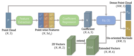
Figure 2: Flowchart of the LGR module. Note that the 2D coordinates are randomly sampled from $\mathcal{D}$ via PDS [6] at each iteration. We refer readers to the supplementary material for the detailed network architecture.

3.2 Geometry-guided UDF Estimation

This module aims to estimate the unsigned distance field of $\mathcal{P}_{M}$, where the iso-surface with the value of zero indicates the surface. As aforementioned, existing learning-based UDF estimation methods, such as NDF [11] and GIFS [38], utilize a neural network to implicitly regress the UDFs from point clouds, thus limiting their accuracy. Besides, the trained models often yield poor results on unseen data. In sharp contrast to the regression-based methods, GUE leverages the inherent geometric property of input point clouds, leading to a more accurate UDF estimation method with better generalizability.

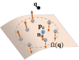
(a)

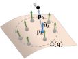
(b)

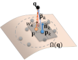
(c)

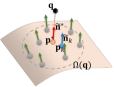
(d)

Figure 3: Illustration of the UDF and its gradient estimation processes. (a) Un-oriented normal vectors. (b) Aligned normal vectors. (c) UDF estimation. (d) UDF gradient estimation.

Formulation of UDF and its gradient estimation. Given a query point $\mathbf{q}\in\mathbb{R}^{3}$, we can find its $K$ nearest points from $\mathcal{P}_{M}$ in a Euclidean distance sense, denoted as $\Omega(\mathbf{q})=\{\mathbf{p}_{k}|\mathbf{p}_{k}\in\mathcal{P}_{R}\}_{k=1}^{K}$. Denote by $\mathbf{n}_{k}$ the un-oriented normal of $\mathbf{p}_{k}$. Before calculating the UDF, as shown in Fig. 3(b), we first align $\{\mathbf{n}_{k}\}_{k=1}^{K}$ with reference to $\mathbf{q}$ via

$$\mathbf{\tilde{n}}_{k}(\mathbf{q})=\texttt{sgn}\left(\langle\mathbf{n}_{k},\mathbf{\tilde{p}}_{k}\rangle\right)\mathbf{n}_{k},\vspace{-0.15cm}$$ (2)

where $\mathbf{\tilde{p}}_{k}:=\mathbf{q}-\mathbf{p}_{k}$, $\langle\cdot,\cdot\rangle$ computes the inner product of two vectors, and $\texttt{sgn}(\cdot)$ extracts the sign of the input. Eq. (2) makes $\mathbf{\tilde{n}}_{k}$ align with $\mathbf{\tilde{p}}_{k}$, i.e., $\langle\mathbf{\tilde{n}}_{k},\mathbf{\tilde{p}}_{k}\rangle>0$.

Denote by $\mathbf{p}^{*}$ the point on surface $\mathcal{S}$ closest to $\mathbf{q}$, and $\mathbf{\tilde{n}}^{*}$ its aligned normal vector. As $\Omega(\mathbf{q})$ generally covers a small region/area shown in Fig. 3(c), we could simply adopt the weighted average of the Euclidean distances between $\mathbf{q}$ and each of $\{\mathbf{p}_{k}\}$, namely point-to-point (P2P) distance, to approximate $\mathbf{q}$’s UDF:

$$\texttt{U}(\mathbf{q})\approx\sum_{\mathbf{p}_{k}\in\Omega(\mathbf{q})}w_{1}(\mathbf{q},\mathbf{p}_{k})\cdot\|\mathbf{\tilde{p}}_{k}\|_{2},\vspace{-0.2cm}$$ (3)

where the weights $\{w_{1}(\mathbf{q},\mathbf{p}_{k})\}_{k=1}^{K}$ are non-negative and satisfying $\sum_{k=1}^{K}w_{1}(\mathbf{q},\mathbf{p}_{k})=1$. However, despite upsampling, $\Omega(\mathbf{q})$ may still be sparse, and the distance of $\mathbf{q}$ to each $\mathbf{p}_{k}$ is much larger than its unsigned distance value, as shown in Fig. 4(a), resulting in a large approximation error.

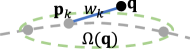
(a)

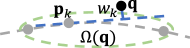
(b)

Figure 4: Visual illustration of the difference between (a) P2P and (b) P2T distances when $\Omega(\mathbf{q})$ is sparse. We also refer readers to Table 5 for the quantitative comparisons.

Instead, we propose to approximate $\texttt{U}(\mathbf{q})$ through the weighted average of the Euclidean distances from $\mathbf{q}$ to the tangent planes of each of $\{\mathbf{p}_{k}\}$, namely point-to-tangent plane (P2T) distance :

$$\texttt{U}(\mathbf{q})\approx\Phi(\mathbf{q}):=\sum_{\mathbf{p}_{k}\in\Omega(\mathbf{q})}w_{1}(\mathbf{q},\mathbf{p}_{k})\cdot\langle\mathbf{\tilde{n}}_{k},\mathbf{\tilde{p}}_{k}\rangle.\vspace{-0.2cm}$$ (4)

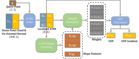
Figure 5: Flowchart of the GUE module. We refer readers to the supplementary material for the detailed network architecture.

Similarly, we propose to approximate the gradient of $\texttt{U}(\mathbf{q})$, denoted as $\nabla\texttt{U}(\mathbf{q})$, using the continuity property of the normal vectors of a surface and the fact $\nabla\texttt{U}(\mathbf{q})=\mathbf{\tilde{n}}^{*}$. See Fig. 3(d). We use $\mathbf{\tilde{n}}_{k}$, each of which is around $\mathbf{\tilde{n}}^{*}$, to approximate $\nabla\texttt{U}(\mathbf{q})$ as

$$\nabla\texttt{U}(\mathbf{q})\approx\Theta(\mathbf{q}):=\frac{\sum_{\mathbf{p}_{k}\in\Omega(\mathbf{q})}w_{2}(\mathbf{q},\mathbf{p}_{k})\cdot\tilde{\mathbf{n}}_{k}}{\|\sum_{\mathbf{p}_{k}\in\Omega(\mathbf{q})}w_{2}(\mathbf{q},\mathbf{p}_{k})\cdot\tilde{\mathbf{n}}_{k}\|},\vspace{-0.15cm}$$ (5)

where the weights $\{w_{2}(\mathbf{q},\mathbf{p}_{k})\}_{k=1}^{K}$ are non-negative and satisfy $\sum_{k=1}^{K}w_{2}(\mathbf{q},\mathbf{p}_{k})=1$.

Learning the weights. Based on the above formulation, the problem of UDF estimation is boiled down to obtaining $\{w_{1}(\mathbf{q},\mathbf{p}_{k}),~{}w_{2}(\mathbf{q},\mathbf{p}_{k})\}_{k=1}^{K}$. As illustrated in Fig. 5, we construct a sub-network to learn them adaptively. Intuitively, the values of the weights should be relevant to the relative position between $\mathbf{q}$ and $\mathbf{p}_{k}$ and the overall shape of $\Omega(\mathbf{q})$. Thus, we embed $\mathbf{\tilde{p}}_{k}$ and $\mathbf{\tilde{n}}_{k}$ via an MLP to obtain point-wise features for all neighbors, $\mathbf{F}_{k}(\mathbf{q})$, which are then maxpooled, leading to a global feature, $\mathbf{F}(\mathbf{q})$, to encode the overall shape of $\Omega(\mathbf{q})$. Finally, we concatenate the above-mentioned features and feed them into two separated MLPs followed with the Softmax layer to regress the two sets of weights.

Remark. Although $\Theta(\mathbf{q})$ could be calculated through the back-propagation (BP) of the neural network (the NDF method [11] adopts this manner), such a process is time-consuming. Compared with BP-based UDF gradient estimation, our method is more efficient. Besides, owing to the separate estimation processes, the UDF error would not be transferred to its gradient, making it more accurate. To the best of our knowledge, this is the first to decouple the estimation processes of UDF and its gradient. See the experimental comparison in Sec. 4.3.

3.3 Edge-based Marching Cube

Inspired by the classic marching cube algorithm [22] that extracts triangles in a cube according to the occupancy of its eight vertices, we propose edge-based marching cube (E-MC) to extract triangle meshes from the predicted unsigned distance field in the preceding module. Generally, we first detect whether the connection between any pair of vertices of a cube intersects with the surface, then find the most matched condition with the detection results from the lookup table of Marching Cube.

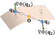
(a)

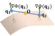
(b)

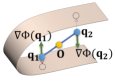
(c)

(d)

Figure 6: The position relationship between the surface and edge. (a) The surface interacts with the edge. (b)(c) The surface does not interact with the edge. (d) One vertex of the edge is extremely close to the surface. See the supplementary material for comprehensive examination of different cases.

Edge intersection detection. As illustrated in Fig. 6, if the surface interacts with the connection between vertices $\mathbf{q}_{1}$ and $\mathbf{q}_{2}$, denoted as $\mathbf{q}_{1}\mathbf{q}_{2}$, the following constraints must be satisfied:

$$\langle\Theta(\mathbf{q}_{1}),\Theta(\mathbf{q}_{2})\rangle<0,$$

$$\langle\Theta(\mathbf{q}_{1}),\overrightarrow{\mathbf{o}\mathbf{q}_{2}}\rangle>0,~{}~{}\langle\Theta(\mathbf{q}_{2}),\overrightarrow{\mathbf{o}\mathbf{q}_{1}}\rangle>0,\vspace{-0.3cm}$$ (6)

where $\mathbf{o}$ is the midpoint between $\mathbf{q}_{1}$ and $\mathbf{q}_{2}$. Specifically, the first constraint indicates the directions of the UDF gradients of $\mathbf{q}_{1}$ and $\mathbf{q}_{2}$ must be opposite, i.e., the angle between them is larger than $90^{\circ}$. The last two constraints ensure that $\mathbf{q}_{1}$ and $\mathbf{q}_{2}$ are located at different sides of an identical part of a surface to eliminate the case shown in Fig. 6(c). Once the above three constraints are satisfied, the intersection of the surface with $\mathbf{q}_{1}\mathbf{q}_{2}$, denoted as $\mathbf{v}(\mathbf{q}_{1},\mathbf{q}_{2})$, can be calculated via

$$\mathbf{v}(\mathbf{q}_{1},\mathbf{q}_{2})=\frac{\mathbf{q}_{2}\Phi(\mathbf{q}_{1})+\mathbf{q}_{1}\Phi(\mathbf{q}_{2})}{\Phi(\mathbf{q}_{1})+\Phi(\mathbf{q}_{2})}.\vspace{-0.15cm}$$ (7)

In addition, if at least one of $\Phi(\mathbf{q}_{1})$ and $\Phi(\mathbf{q}_{2})$ is less than a small threshold $\tau$, their connection is determined to interact with the surface, and the vertex with the smaller UDF is the intersection.

Triangle extraction. After utilizing the edge intersection detection on the connections between any two vertices of a cube, we find the most similar condition to the detection results in the lookup table of Marching Cube to extract the triangles. We refer the readers to the supplementary material for more details.

Remark. With reference to a typical vertex of the 3D cube, MeshUDF [16] converts UDFs to SDFs in a small cube by using only the first constraint of Eq. (3.3). GIFS [38] utilizes a sub-network to determine whether $\mathbf{q}_{1}\mathbf{q}_{2}$ intersects the surface, which is not as general as ours. In Sec. 4.3, we experimentally demonstrate the advantage of our E-MC over MeshUDF.

3.4 Loss Function

We design a joint loss function to train GeoUDF in an end-to-end manner. (1) Loss for upsampling $\mathcal{L}_{\text{PU}}$. We compute the Chamfer Distance (CD) between the upsampled point cloud $\mathcal{P}_{M}$ and its ground-truth dense point cloud to drive the learning of the LGR module. Note that we do not supervise the normal vectors. (2) Losses for UDF and its gradient learning $\mathcal{L}_{\rm UDF}$ and $\mathcal{L}_{\rm Grad}$. We use the mean absolute error between predicted and ground-truth UDFs and the cosine distance between predicted and ground-truth gradients to supervise the learning of the GUE module. The overall loss function is finally written as

$$\mathcal{L}=\lambda_{1}\mathcal{L}_{\rm PU}+\lambda_{2}\mathcal{L}_{\rm UDF}+\lambda_{3}\mathcal{L}_{\rm Grad},\vspace{-0.15cm}$$ (8)

where $\lambda_{1}$, $\lambda_{2}$, and $\lambda_{3}$ are hyper-parameters for balancing the three terms.

4 Experiments

Implementation details. During training, we set the upsampling factor $M=16$. For each shape, we sampled 2048 query points near the surface in one training iteration. We set the size of neighbourhood $K=10$. We trained our framework in two stages: first, we only trained LGR, i.e., $\lambda_{1}=100$ and $\lambda_{2}=\lambda_{3}=0$, with the learning rate $10^{-3}$ for 100 epochs; second, we trained the whole network with $\lambda_{1}=100$, $\lambda_{2}=1$, and $\lambda_{3}=0.1$ for 300 epochs with the learning rate $10^{-4}$. We conducted all experiments on an NVIDIA RTX 3090 GPU with Intel(R) Xeon(R) CPU.

Table 1: Quantitative comparison of different methods on the 13 classes of the ShapeNet dataset. Note that the MC of resolution 128 was applied to all methods for surface reconstruction, except POCO^† and GIFS^†, where the MC resolutions were set to 256 and 160, respectively, to keep the same as their original papers.

Method	Clean				Noisy (0.005)
	CD $(\times 10^{-2})$ $\downarrow$		F-Score $\uparrow$		CD $(\times 10^{-2})$ $\downarrow$		F-Score $\uparrow$
	Mean	Median	$\text{F1}^{0.5\%}$	$\text{F1}^{1\%}$	Mean	Median	$\text{F1}^{0.5\%}$	$\text{F1}^{1\%}$
ONet [25]	$0.894$	$0.716$	$0.535$	$0.756$	$0.875$	$0.764$	$0.642$	$0.785$
CONet [29]	$0.549$	$0.489$	$0.624$	$0.910$	$0.454$	$0.444$	$0.766$	$0.942$
SAP [28]	$0.411$	$0.370$	$0.841$	$0.953$	$0.380$	$0.358$	$0.821$	$0.959$
POCO [5]	0.321	0.283	0.913	0.971	0.369	0.337	0.863	0.965
POCO† [5]	0.290	0.221	0.921	0.985	0.304	0.280	0.875	0.984
DOG [34]	$0.429$	$0.353$	$0.792$	$0.956$	$0.381$	$0.337$	$0.814$	$0.967$
NDF [11]	$0.341$	$0.320$	$0.840$	$0.976$	$0.431$	$0.419$	$0.685$	$0.961$
GIFS [38]	$0.328$	$0.276$	$0.860$	$0.974$	$0.418$	$0.358$	$0.731$	$0.958$
GIFS† [38]	$0.281$	$0.243$	$0.914$	$0.985$	$0.376$	$0.348$	$0.780$	$0.968$
Ours	$\boldsymbol{0.234}$	$\boldsymbol{0.226}$	$\boldsymbol{0.938}$	$\boldsymbol{0.992}$	$\boldsymbol{0.289}$	$\boldsymbol{0.278}$	$\boldsymbol{0.893}$	$\boldsymbol{0.987}$

Figure 7: Visual comparisons on the ShapeNet dataset [8]. We refer readers to the supplementary material for more visual results.

4.1 Watertight Surface Reconstruction

Experiment settings. Following previous works [25, 29, 28, 5], we adopted the ShapeNet Core dataset [8] processed by DISN [37], removing the non-manifold and interior structures of the original shapes. We split the data into the train/val/test sets according to 3D-R2N2 [12]. For each shape, we randomly sampled 3000 points from the surface as the input sparse point cloud. We conducted experiments under two settings, i.e, clean data and noisy data derived by adding the Gaussian noise of standard deviation 0.005 to the clean data. We followed [25, 29, 28, 34] to set the resolution of Marching Cube as 128 for all methods for fair comparisons. To measure reconstruction quality quantitatively, we followed GIFS [38], a UDF-based method, to sample $10^{5}$ points from each reconstructed surface to calculate CD and F-Score with the threshold of 0.5% and 1% with respect to ground-truths.

Comparisons. We compared our GeoUDF with state-of-the-art methods, including ONet [25], CONet [29], SAP [28], POCO [5], DOG [34], NDF [11], and GIFS [38]. On noisy data, we directly applied the pre-trained networks of ONet, CONet, SAP, POCO and DOG released by the authors, which share the same training settings as ours. However, as their pre-trained networks on clean data were not publicly available, we used their offical codes to retrain them with the same settings as ours for fair comparisons. Besides, as the pre-trained networks of NDF and GIFS were trained only with the ShapeNet car dataset rather than the whole dataset, we retrained them on the whole dataset for fair comparisons.

We quantitatively compared those methods in Table 1, where it can be seen that our method outperforms the other methods in terms of all metrics, even POCO and GIFS with larger Marching Cube resolution. Besides, as illustrated in Fig. 7, our GeoUDF can reconstruct surfaces with sharp edges and correct structures that are closer to GTs.

Figure 8: Visual comparisons on the MGN dataset [4].   Zoom in to see details.

Figure 9: Visual comparisons of different surface reconstruction methods on the ScanNet dataset [13].

4.2 Unseen Non-watertight Surface Reconstruction

Dataset and Metrics. Following GIFS [38], we evaluated our method on the MGN [4] and the raw ShapeNet car [8] datasets, containing the shapes with boundaries and interior structures. Besides, we also evaluated our method on the ScanNet dataset [13], in which the point clouds were collected through an RGB-D camera from the real scenes. For the MGN dataset, we randomly sampled 3000 points from the surface as the input. As for the shapes and scenes in the ShapeNet car and ScanNet dataset, we randomly sampled 6000 points from the surface or the dense point cloud as the input.

Comparisons. To verify the generalizability, for all methods, we used the trained models on the ShapeNet dataset (watertight shapes) to perform inference directly. As shown in Table 2, Figs. 8 and 10, our GeoUDF exceeds GIFS [38] both quantitatively and visually on the MGN and ShapeNet car datasets. Besides, Fig. 9 visualizes the results of different methods on the ScanNet dataset, where it can be seen that CONet [29] and POCO [5] fail to reconstruct the whole scene; GIFS can reconstruct the objects in the scene, but the details are not well preserved. By contrast, the surfaces by our GeoUDF contain more details and are closer to GT ones.

Figure 10: Visual comparisons on the ShapeNet cars.

Table 2: Quantitative comparisons on the MGN and ShapeNet car dataset.

Dataset	Method	CD ($\times 10^{-2}$) $\downarrow$		F-Score $\uparrow$
		Mean	Media	$\text{F1}^{0.5\%}$	$\text{F1}^{1\%}$
MGN	GIFS [38]	$0.248$	$0.234$	$0.951$	$0.991$
	Ours	$\boldsymbol{0.194}$	$\boldsymbol{0.190}$	$\boldsymbol{0.975}$	$\boldsymbol{0.996}$
ShapeNet Car	GIFS [38]	$0.408$	$0.346$	$0.758$	$0.954$
	Ours	$\boldsymbol{0.310}$	$\boldsymbol{0.271}$	$\boldsymbol{0.870}$	$\boldsymbol{0.986}$

4.3 Ablation Study

We conducted comprehensive ablation studies on the ShapeNet dataset to better understand our framework.

Advantage of LGR. We evaluated the upsampling function of our LGR module on the ShapeNet [8] dataset with $M=16$ and compared with recent representative PU methods, i.e., PUGeo-Net [32], MAFU [33], and NP [15]. For a fair comparison, we retrained the official codes of the compared methods with the same training data as ours. As listed in Table 3, it can be seen that our method with the fewest number of parameters achieves the best performance. NP is much worse than others because its modeling manner makes it hard to deal with very sparse point clouds. Besides, Fig. 11 visually compares the results of different methods, further demonstrating the advantage of our LRG. We also refer readers to the supplementary material for the results of LGR achieved by the 3^rd-order polynomial.

Table 3: Comparisons of different PU methods ($M=16$). P2F: point-to-face distance.

Methods	# Param	Normal Supervision	CD ($\downarrow$) ($\times 10^{-2}$)	P2F ($\downarrow$) ($\times 10^{-3}$)
PUGeo [32]	1.287M	Yes	$0.287$	$1.309$
MAFU [33]	1.390M	No	$0.289$	$1.220$
NP [15]	0.637M	Yes	$0.493$	$4.572$
Ours	0.522M	No	$\boldsymbol{0.245}$	$\boldsymbol{0.512}$

Figure 11: Visual comparison of the results by different upsampling methods on the ShapeNet dataset [8].

Necessity of LGR. We removed LGR from our GeoUDF to reconstruct surfaces from input sparse point clouds directly. Under this scenario, we estimated the normal vectors by using the principal component analysis (PCA). Besides, we also equipped GIFS [38] with our LGR, i.e., input point clouds were upsampled by our LGR before voxelization. From Table 4, it can be seen that LRG can boost the reconstruction accuracy of both GIFS and ours, validating its effectiveness. Besides, as visualized in Fig. 12, without LGR, the reconstructed surfaces are much worse, i.e., there are many holes caused by the sparsity of the input point cloud.

Figure 12: Visual results of our method w/ and w/o LGR.

Table 4: The reconstruction accuracy of GIFS [38] and our method with and without LGR.

Method	L1-CD $(\times 10^{-2})$ $\downarrow$		F-Score $\uparrow$
	Mean	Median	$\text{F1}^{0.5\%}$	$\text{F1}^{1\%}$
GIFS	0.328	0.276	0.860	0.974
GIFS w/ LGR	0.316	0.292	0.894	0.981
Ours w/o LGR	0.284	0.264	0.882	0.967
Ours	0.234	0.226	0.938	0.992

Accuracy of UDF and its gradient estimation. The accuracy of reconstructed surfaces cannot exactly reflect that of UDFs and corresponding gradients due to the discrete cubes of MC. Thus, we directly compared the accuracy of UDFs and gradients estimated by different methods. In addition to NDF [11] and GIFS [38] for comparison, we also set another three baselines (named Regress, P2P and BP). Regress replaces Eqs. (4) and (5) of our GUE with two separated MLPs to regress UDFs and gradients, and P2P utilizes Eq. (3) to calculate UDF as described before. BP utilizes the back propagation of the network to calculate the gradient. As listed in Table 5, our GUE produces the most accurate UDFs and gradients. moreover, the error is much smaller than the edge length of the cube of E-MC (1/127). Besides, BP can obtain gradients that are slightly worse than those of our GUE, but it is much slower. Finally, we validated that the shape encoding (SE) of $\Omega(\mathbf{q})$ is essential to our GUE, i.e., GUE w/o SE produces UDFs and gradients with much larger error than GUE.

Table 5: UDF accuracy of different methods. Note that GIFS does not rely on the gradients of UDFs.

UDF Estimation	UDF Error $\downarrow$		Time $\downarrow$ ($\upmu$s/point)
	UDF $(\times 10^{-3})$	Grad $(^{\circ})$
NDF [11]	2.536	13.930	1.173
GIFS [38]	2.439	-	4.228
Regress	0.994	8.371	1.762
P2P	1.240	7.238	3.497
BP	0.615	7.877	12.125
GUE w/o SE	1.453	10.707	1.271
GUE	0.615	7.237	3.405

Size of $\Omega(\mathbf{q})$. From Table 6, we can conclude that our GeoUDF is robust to the size of neighborhood used in Eqs. (4) and (5). This is credited to the manner of learning adaptive weights, i.e., very smaller weights would be predicted for not important neighbours.

Table 6: The reconstruction accuracy of different $K$-NN sizes.

$K$	CD ($\times 10^{-2}$) $\downarrow$		F-Score $\uparrow$
	Mean	Median	$\text{F1}^{0.5\%}$	$\text{F1}^{1\%}$
5	$0.235$	$0.227$	$0.937$	$0.992$
10	$0.234$	$0.226$	$0.938$	$0.992$
20	$0.232$	$0.224$	$0.939$	$0.993$

Superiority of E-MC. We also compared our E-MC with MeshUDF [16], the SOTA method for extracting triangle meshes from unsigned distance fields. For a fair comparison, we fed the two methods with identical unsigned distance fields estimated by our GUE. From Table 7, it can be seen that our E-MC can extract triangle meshes with higher quality than MeshUDF. Besides, we also studied how the resolution of the 3D grid affects reconstruction accuracy. From Table 8, we can see that the reconstruction accuracy gradually improves with the resolution increasing, which is consistent with the visual results in Fig. 13, but more times are consumed. Such an observation is fundamentally credited to the highly-accurate UDFs by our method.

Table 7: Quantitative comparison of our E-MC with MeshUDF [16].

Method	CD ($\times 10^{-2}$) $\downarrow$		F-Score $\uparrow$
	Mean	Median	$\text{F1}^{0.5\%}$	$\text{F1}^{1\%}$
GUE+MeshUDF [16]	$0.266$	$0.251$	$0.916$	$0.978$
GUE+E-MC	$\boldsymbol{0.234}$	$\boldsymbol{0.226}$	$\boldsymbol{0.938}$	$\boldsymbol{0.992}$

Figure 13: Visual illustration of the effect of the resolution of E-MC on the reconstructed surface.

Table 8: The reconstruction accuracy under various 3D grid resolutions used in E-MC.

Res.	CD ($\times 10^{-2}$) $\downarrow$		F-Score $\uparrow$		Time (s) $\downarrow$
	Mean	Median	$\text{F1}^{0.5\%}$	$\text{F1}^{1\%}$	UDF	E-MC
32	$0.584$	$0.554$	$0.646$	$0.824$	0.051	3.295
64	$0.312$	$0.285$	$0.860$	$0.958$	0.138	4.744
128	$0.234$	$0.226$	$0.938$	$0.992$	0.759	15.282
192	$0.223$	$0.218$	$0.949$	$0.995$	2.264	32.052

4.4 Efficiency Analysis

We also evaluated the efficiency of our GeoUDF on the ShapeNet dataset. As listed in Table 9, our method has the fewest number of parameters while achieving the highest reconstruction accuracy among all methods, which is credited to our explicit and elegant formulations to this problem. We also evaluated the time consumption of our method, demonstrating that all modules before surface extraction are very efficient. As for the surface extraction process, due to the global optimization in our E-MC, it is slower than the traditional Marching Cube methods, but faster than GIFS.

Table 9: Efficiency comparisons. The time of “Inference” refers to the overall time minus the time for iso-surface extraction.

Method	# Param	Time (s) $\downarrow$
		Inference	Surface Extraction
ONet [25]	10.373M	0.653	0.219
CONet [29]	1.978M	0.941	0.589
SAP [28]	1.085M	0.247	0.384
POCO [5]	12.790M	4.652	8.560
DOG [34]	2.182M	0.302	0.228
GIFS [38]	3.682M	27.771	26.915
Ours	0.775M	0.759	15.282

5 Conclusion

GeoUDF is a novel learning-based framework for reconstructing surfaces from sparse 3D point clouds. It has several advantages, including being lightweight, efficient, accurate, explainable, and generalizable, which have been validated through extensive experiments and ablation studies. The various advantages of our framework are fundamentally credited to the explicit and elegant formulations of the problems of UDF and its gradient estimation and local structure representation from the geometric perspective, as well as the edge-based marching cube.

References

- [1] Ma Baorui, Han Zhizhong, Liu Yu-Shen, and Zwicker Matthias. Neural-pull: Learning signed distance functions from point clouds by learning to pull space onto surfaces. In International Conference on Machine Learning, volume 139, pages 7246–7257, 2021.
- [2] Jan Bednarik, Shaifali Parashar, Erhan Gundogdu, Mathieu Salzmann, and Pascal Fua. Shape reconstruction by learning differentiable surface representations. In Proceedings of the IEEE/CVF Conference on Computer Vision and Pattern Recognition, pages 4716–4725, June 2020.
- [3] Fausto Bernardini, Joshua Mittleman, Holly Rushmeier, Cláudio Silva, and Gabriel Taubin. The ball-pivoting algorithm for surface reconstruction. IEEE transactions on visualization and computer graphics, 5(4):349–359, 1999.
- [4] Bharat Lal Bhatnagar, Garvita Tiwari, Christian Theobalt, and Gerard Pons-Moll. Multi-garment net: Learning to dress 3d people from images. In Proceedings of the IEEE/CVF International Conference on Computer Vision, pages 5420–5430, October 2019.
- [5] Alexandre Boulch and Renaud Marlet. Poco: Point convolution for surface reconstruction. In Proceedings of the IEEE/CVF Conference on Computer Vision and Pattern Recognition, pages 6302–6314, June 2022.
- [6] Robert Bridson. Fast poisson disk sampling in arbitrary dimensions. In ACM SIGGRAPH 2007 sketches, pages 22–es. 2007.
- [7] Rohan Chabra, Jan E Lenssen, Eddy Ilg, Tanner Schmidt, Julian Straub, Steven Lovegrove, and Richard Newcombe. Deep local shapes: Learning local sdf priors for detailed 3d reconstruction. In European Conference on Computer Vision, pages 608–625. Springer, 2020.
- [8] Angel X Chang, Thomas Funkhouser, Leonidas Guibas, Pat Hanrahan, Qixing Huang, Zimo Li, Silvio Savarese, Manolis Savva, Shuran Song, Hao Su, et al. Shapenet: An information-rich 3d model repository. arXiv preprint arXiv:1512.03012, pages 1–xxx, 2015.
- [9] Jiawen Chen, Dennis Bautembach, and Shahram Izadi. Scalable real-time volumetric surface reconstruction. ACM Transactions on Graphics), 32(4):1–16, 2013.
- [10] Julian Chibane, Thiemo Alldieck, and Gerard Pons-Moll. Implicit functions in feature space for 3d shape reconstruction and completion. In Proceedings of the IEEE/CVF Conference on Computer Vision and Pattern Recognition, pages 6970–6981, June 2020.
- [11] Julian Chibane, Gerard Pons-Moll, et al. Neural unsigned distance fields for implicit function learning. Advances in Neural Information Processing Systems, 33:21638–21652, 2020.
- [12] Christopher B Choy, Danfei Xu, JunYoung Gwak, Kevin Chen, and Silvio Savarese. 3d-r2n2: A unified approach for single and multi-view 3d object reconstruction. In European conference on computer vision, pages 628–644. Springer, 2016.
- [13] Angela Dai, Angel X. Chang, Manolis Savva, Maciej Halber, Thomas Funkhouser, and Matthias Niessner. Scannet: Richly-annotated 3d reconstructions of indoor scenes. In Proceedings of the IEEE Conference on Computer Vision and Pattern Recognition, pages 5828–5839, July 2017.
- [14] Manfredo P Do Carmo. Differential geometry of curves and surfaces: revised and updated second edition. Courier Dover Publications, 2016.
- [15] Wanquan Feng, Jin Li, Hongrui Cai, Xiaonan Luo, and Juyong Zhang. Neural points: Point cloud representation with neural fields for arbitrary upsampling. In Proceedings of the IEEE/CVF Conference on Computer Vision and Pattern Recognition, pages 18633–18642, June 2022.
- [16] Benoit Guillard, Federico Stella, and Pascal Fua. Meshudf: Fast and differentiable meshing of unsigned distance field networks. In European Conference on Computer Vision, pages 576–592, 2022.
- [17] Hugues Hoppe. Poisson surface reconstruction and its applications. In Proceedings of the 2008 ACM symposium on Solid and physical modeling, pages 10–10, 2008.
- [18] Michael Kazhdan and Hugues Hoppe. Screened poisson surface reconstruction. ACM Transactions on Graphics, 32(3):1–13, 2013.
- [19] Ravikrishna Kolluri. Provably good moving least squares. ACM Transactions on Algorithms, 4(2):1–25, 2008.
- [20] Ruihui Li, Xianzhi Li, Chi-Wing Fu, Daniel Cohen-Or, and Pheng-Ann Heng. Pu-gan: A point cloud upsampling adversarial network. In Proceedings of the IEEE/CVF International Conference on Computer Vision, pages 7203–7212, October 2019.
- [21] Shi-Lin Liu, Hao-Xiang Guo, Hao Pan, Peng-Shuai Wang, Xin Tong, and Yang Liu. Deep implicit moving least-squares functions for 3d reconstruction. In Proceedings of the IEEE/CVF Conference on Computer Vision and Pattern Recognition, pages 1788–1797, June 2021.
- [22] William E Lorensen and Harvey E Cline. Marching cubes: A high resolution 3d surface construction algorithm. ACM siggraph computer graphics, 21(4):163–169, 1987.
- [23] Baorui Ma, Yu-Shen Liu, and Zhizhong Han. Reconstructing surfaces for sparse point clouds with on-surface priors. In Proceedings of the IEEE/CVF Conference on Computer Vision and Pattern Recognition, pages 6315–6325, June 2022.
- [24] Aihua Mao, Zihui Du, Junhui Hou, Yaqi Duan, Yong-jin Liu, and Ying He. Pu-flow: A point cloud upsampling network with normalizing flows. IEEE Transactions on Visualization and Computer Graphics, pages 1–14, 2022.
- [25] Lars Mescheder, Michael Oechsle, Michael Niemeyer, Sebastian Nowozin, and Andreas Geiger. Occupancy networks: Learning 3d reconstruction in function space. In Proceedings of the IEEE/CVF Conference on Computer Vision and Pattern Recognition, pages 4460–4470, June 2019.
- [26] Philipp Mittendorfer and Gordon Cheng. 3d surface reconstruction for robotic body parts with artificial skins. In 2012 IEEE/RSJ International Conference on Intelligent Robots and Systems, pages 4505–4510, 2012.
- [27] Jeong Joon Park, Peter Florence, Julian Straub, Richard Newcombe, and Steven Lovegrove. Deepsdf: Learning continuous signed distance functions for shape representation. In Proceedings of the IEEE/CVF Conference on Computer Vision and Pattern Recognition, pages 165–174, June 2019.
- [28] Songyou Peng, Chiyu Jiang, Yiyi Liao, Michael Niemeyer, Marc Pollefeys, and Andreas Geiger. Shape as points: A differentiable poisson solver. Advances in Neural Information Processing Systems, 34:13032–13044, 2021.
- [29] Songyou Peng, Michael Niemeyer, Lars Mescheder, Marc Pollefeys, and Andreas Geiger. Convolutional occupancy networks. In European Conference on Computer Vision, pages 523–540. Springer, 2020.
- [30] Charles Ruizhongtai Qi, Li Yi, Hao Su, and Leonidas J Guibas. Pointnet++: Deep hierarchical feature learning on point sets in a metric space. Advances in neural information processing systems, 30:1–xxx, 2017.
- [31] Guocheng Qian, Abdulellah Abualshour, Guohao Li, Ali Thabet, and Bernard Ghanem. Pu-gcn: Point cloud upsampling using graph convolutional networks. In Proceedings of the IEEE/CVF Conference on Computer Vision and Pattern Recognition, pages 11683–11692, June 2021.
- [32] Yue Qian, Junhui Hou, Sam Kwong, and Ying He. PUGeo-Net: A geometry-centric network for 3D point cloud upsampling. In European conference on computer vision, pages 752–769. Springer, 2020.
- [33] Yue Qian, Junhui Hou, Sam Kwong, and Ying He. Deep magnification-flexible upsampling over 3d point clouds. IEEE Transactions on Image Processing, 30:8354–8367, 2021.
- [34] Peng-Shuai Wang, Yang Liu, and Xin Tong. Dual octree graph networks for learning adaptive volumetric shape representations. ACM Transactions on Graphics, 41(4):1–15, 2022.
- [35] Yue Wang, Yongbin Sun, Ziwei Liu, Sanjay E Sarma, Michael M Bronstein, and Justin M Solomon. Dynamic graph cnn for learning on point clouds. Acm Transactions On Graphics, 38(5):1–12, 2019.
- [36] Yifan Wang, Shihao Wu, Hui Huang, Daniel Cohen-Or, and Olga Sorkine-Hornung. Patch-based progressive 3d point set upsampling. In Proceedings of the IEEE/CVF Conference on Computer Vision and Pattern Recognition, pages 5958–5967, June 2019.
- [37] Qiangeng Xu, Weiyue Wang, Duygu Ceylan, Radomir Mech, and Ulrich Neumann. Disn: Deep implicit surface network for high-quality single-view 3d reconstruction. Advances in Neural Information Processing Systems, 32:1–xxx, 2019.
- [38] Jianglong Ye, Yuntao Chen, Naiyan Wang, and Xiaolong Wang. Gifs: Neural implicit function for general shape representation. In Proceedings of the IEEE/CVF Conference on Computer Vision and Pattern Recognition, pages 12829–12839, June 2022.
- [39] Lequan Yu, Xianzhi Li, Chi-Wing Fu, Daniel Cohen-Or, and Pheng-Ann Heng. Pu-net: Point cloud upsampling network. In Proceedings of the IEEE Conference on Computer Vision and Pattern Recognition, pages 2790–2799, June 2018.
- [40] Junsheng Zhou, Baorui Ma, Yu-Shen Liu, Yi Fang, and Zhizhong Han. Learning consistency-aware unsigned distance functions progressively from raw point clouds. arXiv preprint arXiv:2210.02757, pages 1–xxx, 2022.