Extracting GHZ states from linear cluster states

Abstract

Quantum information processing architectures typically only allow for nearest-neighbour entanglement creation. In many cases, this prevents the direct generation of $\mathrm{GHZ}$ states, which are commonly used for many communication and computation tasks. Here, we show how to obtain $\mathrm{GHZ}$ states between nodes in a network that are connected in a straight line, naturally allowing them to initially share linear cluster states. We prove a strict upper bound of $\lfloor(n+3)/2\rfloor$ on the size of the set of nodes sharing a $\mathrm{GHZ}$ state that can be obtained from a linear cluster state of $n$ qubits, using local Clifford unitaries, local Pauli measurements, and classical communication. Furthermore, we completely characterize all selections of nodes below this threshold that can share a $\mathrm{GHZ}$ state obtained within this setting. Finally, we demonstrate these transformations on the IBMQ Montreal quantum device for linear cluster states of up to $n=19$ qubits.

I Introduction

Recent years have seen exciting developments in quantum computation and communication, both in theory and experiment. Building upon the year-long research on bipartite settings, focus has now also turned towards multipartite settings, where multiple vertices in a network share quantum resources between them. While the correlations of Greenberger-Horne-Zeilinger ($\mathrm{GHZ}$) states Greenberger et al. (1989) have naturally been the first to explore, other types of graph states Hein et al. (2006) have also been extensively examined Schlingemann (2004); Hein et al. (2004); Bouchet (1988); Hahn et al. (2022). The possible transformations between quantum states is a topic that is heavily studied Briegel and Raussendorf (2001); Van den Nest et al. (2004, 2005); Dahlberg and Wehner (2018); Dahlberg et al. (2020a), and while several hardness results have emerged Dahlberg et al. (2020b, c), a lot of practical questions remain unanswered.

But why should we be interested in transforming one quantum state to another in the first place? One reason can be that it is not always possible to create the exact state that is necessary to perform a specific task, and we need to ‘retrieve’ it from some other state that is more practical to build. For example, while the underlying network architecture might allow for nearest-neighbour interactions, it might not allow for the direct distribution of large $\mathrm{GHZ}$ states between distant parties. Here we show that there is an indirect remedy for this deficiency using suitable transformations of the distributed quantum states. We focus on the transformation of linear cluster states Briegel and Raussendorf (2001), that arise naturally in linear networks. In particular we investigate the transformation to $\mathrm{GHZ}$ states, which are widely used in many quantum communication tasks including anonymous transmission Christandl and Wehner (2005), secret sharing Hillery et al. (1999); Broadbent et al. (2009) and (anonymous) conference key agreement Murta et al. (2020); Hahn et al. (2020); Grasselli et al. (2022).

Such transformations require the removal of some of the qubits from the state by measuring them, such that only a selected subset of the qubits of the resource linear cluster state can in the end belong to the target $\mathrm{GHZ}$ state. We refer to these transformations as $\mathrm{GHZ}$ extractions. A previous study Hahn et al. (2019) showed how to extract three- and four-partite $\mathrm{GHZ}$ states from linear cluster states. Moreover, other works Frantzeskakis et al. (2022); Mannalath and Pathak (2022) study a specific selection of the qubits of an odd-partite resource state. Here, we conclude this study by providing a complete characterisation of which $\mathrm{GHZ}$ extractions are possible and which are not. Very importantly, we provide a tight upper bound to the size of the largest $\mathrm{GHZ}$ state that can be extracted, equal to $\lfloor(n+3)/2\rfloor$; interestingly this is slightly higher than the bound of $n/2$ conjectured in Ref. Briegel and Raussendorf (2001) and than the sizes of the states extracted in the aforementioned studies Frantzeskakis et al. (2022); Mannalath and Pathak (2022). In addition to our theoretical analysis, we perform demonstrations of implementations of the $\mathrm{GHZ}$ extractions from linear cluster states with $n\in\{5,7,\dots,19\}$ qubits on the IBMQ Montreal device.

Our manuscript is organized as follows: The notation, technical terminology and main definitions are introduced in Section II. Section III contains the main theoretical results. In Section IV, the demonstrations are introduced, discussed, and their results presented. Finally, Section V discusses the obtained results and the opportunities for future research. The technical details are diverted to topical appendices: Appendix A contains the proof of an important lemma stated in the theoretical section, Appendix B contains technical details regarding the post-processing steps during the extractions, and Appendix C contains technical details regarding the data analysis of the demonstrations section.

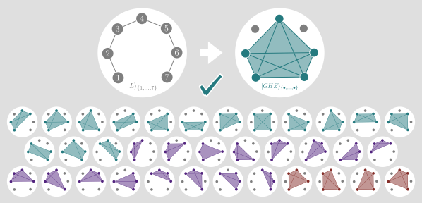
Figure 1: Example of extracting $\mathrm{GHZ}$ states from a linear cluster state with seven qubits: The only $5$-partite $\mathrm{GHZ}$ state that can be extracted from this resource is on the qubits corresponding to $1,2,4,6,7$ and is highlighted in green. For $4$-partite $\mathrm{GHZ}$ states, we also highlight all $15$ possible extraction patterns in green, while the patterns in brown are impossible due to Lemma 1 and the patterns shown in violet are impossible due to both Corollary 1 and Lemma 1. Note that due to Theorem 1 it is impossible to extract $\mathrm{GHZ}$ states with six or more qubits from this resource – it is however trivially possible to extract all combinations of three-partite $\mathrm{GHZ}$ states.

II Notation and terminology

In this work, two quantum graph states play a central role: we define linear cluster states $\ket{\mathrm{L}}$ and GHZ states $\ket{\mathrm{GHZ}}$ as

$$\begin{split}\ket{\mathrm{L}}_{\{1,\dots,n\}}&\mathrel{\mathop{:}}=\frac{1}{2^{n}}\bigotimes_{i=1}^{n}\left(\ket{0}+\ket{1}\sigma_{z}^{i+1}\right)\\ \ket{\mathrm{GHZ}}_{\{1,\dots,m\}}&\mathrel{\mathop{:}}=\frac{1}{\sqrt{2}}\left(\bigotimes_{i=1}^{m}\ket{0}+\bigotimes_{i=1}^{m}\ket{1}\right)\end{split}$$ (1)

and $\ket{\mathrm{L}}_{V}$, $\ket{\mathrm{GHZ}}_{V}$ as the states corresponding to the vertex set $V$. When context permits, with e.g. $\ket{\mathrm{L}}_{n}$ we denote the linear cluster state of size $n$.

Our resource state is the $n$-partite linear cluster state $\ket{\mathrm{L}}_{V_{L}}$. As a graph state it corresponds to a line graph on the vertices $V_{L}{}\mathrel{\mathop{:}}=\{1,2,\ldots,n\}$. Here, each vertex $i$ corresponds to the $i$-th qubit of $\ket{\mathrm{L}}_{V_{L}}$ and the edges of the graph correspond to nearest-neighbour entangling controlled phase gates. This structure allows us to use the terms left and right neighbours of $i$ to indicate any vertices $h$, $j$ with $h<i$, $i<j$, respectively; e.g. the direct left and right neighbours of $i$ are $i\pm 1$.

Let $V_{G}{}\subset V_{L}{}$ be a set of vertices for which we can extract a $\mathrm{GHZ}$ state from the linear cluster resource state. Performing Pauli measurements on the qubits corresponding to $V_{M}\mathrel{\mathop{:}}=V_{L}\setminus V_{G}{}$, we obtain a post-measurement state which is local-Clifford equivalent to the $\ket{\mathrm{GHZ}}_{V_{G}{}}$ state. By performing local operations based on the measurement outcomes, the state can then be locally transformed into this $\mathrm{GHZ}$ state.

This construction allows for $V_{G}$ to inherit the neighbour structure from the linear network $V_{L}{}$: For a vertex $j\in V_{G}{}$, we use $j_{-}$ and $j_{+}$ to indicate the left and right neighbour of $j$ in $V_{G}$, respectively. We refer to the smallest and largest element of $V_{G}$ as the boundaries of the $\mathrm{GHZ}$ state. We finally define any selection of consecutive vertices $i,i+1,\dots,i+k\in V_{G}{}$ as a $k$-island.

III Main results

We now examine what are the different types of $\mathrm{GHZ}$ states one can obtain from a given linear cluster state. We first provide an upper bound for the size $\absolutevalue{V_{G}{}}$ of the extracted $\mathrm{GHZ}$ state, and we then show how to saturate it. In order to achieve this, we use Lemma 1, which provides an impossibility result for $2$-islands (the proof can be found in App. A).

Lemma 1.

No $2$-island can have both a left and a right neighbour in $V_{G}$. If two vertices $i,i+1$ are in $V_{G}{}$, then there is either no vertex to the left of $i$ or no vertex to the right of $i+1$.

Lemma 1 implies that all vertices $i$ in the target $\mathrm{GHZ}$ state must be ‘isolated’ in the linear cluster state; $i-1$ and $i+1$ cannot be in $V_{G}{}$ (with the exception of the boundaries). A corollary for $3$-islands follows directly:

Corollary 1.

If $V_{G}$ contains a $3$-island, then $\absolutevalue{V_{G}{}}{}=3$.

Proof.

Let $i,i+1,i+2$ be a $3$-island in $V_{G}{}$ and assume that $|V_{G}{}|\geq 4$, i.e. that we have $h<i$ or $j>i+2$ in $V_{G}$. This implies that either $i,i+1$ form a $2$-island with both left-neighbour $h$ and right-neighbour $i+2$ or $i+1,i+2$ form a $2$-island with both left-neighbour $i$ and right-neighbour $j$. Both are in direct contradiction to Lemma 1. ∎

By the same argument, $k$-islands with $k\geq 4$ are impossible. Ultimately, such $k$-islands would contain $3$-islands in contradiction to Corollary 1. Figure 1 illustrates examples.

This allows us to calculate the upper bound to $\absolutevalue{V_{G}{}}{}$.

Theorem 1.

The size of a $\mathrm{GHZ}$ state extractable from an $n$-partite linear cluster state via local Clifford operations, local Pauli measurements, and local unitary corrections, is upper-bounded as $\absolutevalue{V_{G}{}}\leq\left\lfloor\frac{n+3}{2}\right\rfloor$.

Proof.

As there are at most two $2$-islands, for every other $i$ in $V_{G}{}$ both $i\pm 1$ were measured. Thus, to maximize $\absolutevalue{V_{G}{}}$, we may have $1,2,n-1,n$ in $V_{G}{}$, and $V_{M}{}$ containing every other vertex in between: For $n$ odd, $V_{M}{}=\{3,5,\dots,n-2\}$; for $n$ even $V_{M}{}=\{3,5,\dots,n-5,n-3,n-2\}$ . In the even case, $n-2$ must be measured due to Corollary 1. In both cases $\absolutevalue{V_{G}{}}{}=n-|V_{M}{}|$ is upper bounded by $\left\lfloor\frac{n+3}{2}\right\rfloor$. ∎

For example, the largest $\mathrm{GHZ}$ state that can be extracted from the $7$-qubit linear cluster state shown in Figure 1 is the $\ket{\mathrm{GHZ}}_{5}$ state where $V_{G}{}=\{1,2,4,6,7\}$ and $V_{M}{}=\{3,5\}$. Figure 1 further shows all possible and impossible selections of $V_{G}$ to extract the $\ket{\mathrm{GHZ}}_{4}$ state.

We now show that there is a set of measurements that saturates the bound of Theorem 1 by explicitly giving such a measurement pattern. For $n\leq 5$ this pattern was shown in Ref. Hahn et al. (2019). For the general case, let us consider a case distinction with respect to the parity of $n$:

First, for odd $n$ we can choose $V_{M}=\{2i+1\}_{i=1}^{\frac{n-3}{2}}$ and every corresponding qubit to be measured in the $\sigma_{x}$-basis; we refer to this measurement pattern as the maximal pattern. Below, we show that this pattern actually gets the desired $\mathrm{GHZ}$ state.

The linear cluster state is a stabilizer state, i.e. it is an element of the shared $+1$ eigenspace of the operators $\{l_{i}=\sigma_{z}^{i-1}\sigma_{x}^{i}\sigma_{z}^{i+1}\}_{i\in V_{L}}$, where $\sigma_{z}^{0}$ and $\sigma_{z}^{n+1}$ are set equal to the identity. This set of operators forms the set of canonical generators of an Abelian subgroup of the $n$-qubit Pauli group known as the stabilizer of the linear cluster states. For an overview of the stabilizer formalism and stabilizer measurements in particular see Gottesman (1997), Gottesman (1998).

Consider the generator transformation

$$l_{2}\rightarrow l_{2}^{{}^{\prime}}=l_{2}l_{4}\dots l_{n-4}l_{n-2}\mathrel{\mathop{:}}=\sigma_{z}^{1}\sigma_{z}^{n}\prod_{2i\in V_{L}}\sigma_{x}^{2i},$$ (2)

which ensures that $l^{{}^{\prime}}_{2}$ and all odd-indexed generators commute with all measurement operators $\{\sigma_{x}^{j_{0}}\}_{j_{0}\in V_{M}{}}$. The post-measurement state is determined by replacing the other $\absolutevalue{V_{M}{}}$ generators $\{l_{2i}\}_{i=2}^{\frac{n-1}{2}}$ with the measurement operators –together with a multiplicative phase depending on the respective measurement outcome. Then (after removing the support on the measured qubits and applying a Hadamard transformation to $1$ and $n$) the post measurement state on $V_{G}$ is characterized by the generators $\sigma_{x}^{V_{G}{}}$ and $\{m_{j_{0}}\sigma_{z}^{j_{0}}\sigma_{z}^{j_{0+}}\}_{j_{0}\in V_{G}{}\setminus\{n\}}$, where the $m_{j_{0}}=\pm 1$ are phases due to the measurement outcomes. These phases can be accounted for by applying $\sigma_{x}$-operations to a selection of the nodes, recovering the generators of the $\ket{\mathrm{GHZ}}_{V_{G}{}}$ state. The number of measurements implies $\absolutevalue{V_{G}{}}{}=n-\absolutevalue{\{3,5,\dots,n-2\}}=\frac{n+3}{2}$ which saturates the bound for odd $n$.

Second, for even $n$ it suffices to observe that a $\sigma_{z}$-measurement on the qubit corresponding to $n$ yields a linear cluster state $\ket{\mathrm{L}}_{\{1,2,\dots,n-1\}}$ up to a randomized $\sigma_{z}^{n-1}$-correction depending on the measurement outcome. In analogy to the odd parity case we then obtain $V_{M}=\{3,5,\dots,n-3,n\}$ such that $\absolutevalue{V_{G}{}}{}=n-\absolutevalue{V_{M}{}}{}=\frac{n+2}{2}=\left\lfloor\frac{n+3}{2}\right\rfloor$ for even $n$.

Note that the even-case analysis above also applies for measuring an ‘internal’ node in the $\sigma_{y}$-basis, rather than the first or last; this does introduce a Clifford rotation on the two neighbours of the node which needs to be accounted for git (2022). The resulting state is then also LOCC equivalent to an ($n-1$)-partite linear cluster state on the remaining nodes, from which in turn a $\ket{\mathrm{GHZ}}_{\frac{n+2}{2}}$ state can be extracted through the maximal pattern. This approach can be extended to more measurements, where additional ‘inside’ nodes are measured in the $\sigma_{y}$-basis, and ‘outside’ nodes are measured in the $\sigma_{z}$-basis. It is straightforward to see that any choice $V_{G}$ allowed by Lemma 1 can be seen as arising from such a setting.

Finally, note that while Lemma 1 does allow $2$-islands on the boundaries of the extracted $\mathrm{GHZ}$ states, they do not necessarily have to be contained in them. For example, $\ket{\mathrm{GHZ}}_{\{1,3,5,7\}}$ can be extracted from $\ket{\mathrm{L}}_{\{1,\ldots,7\}}$ as shown in Figure 1. Rigorously stated, this pattern does not arise from one of the maximal patterns defined above, but can instead be considered as a maximal pattern $\ket{\mathrm{GHZ}}_{\{0,1,3,5,7,8\}}$ extracted from $\ket{\mathrm{L}}_{\{0,\ldots,8\}}$. Here, the additional qubits corresponding to $0$ and $8$ are just “virtual” and not really there; they simply help visualize all possible patterns: $\ket{\mathrm{GHZ}}_{\{1,3,5,7\}}$ can be extracted from the “virtual” state $\ket{\mathrm{GHZ}}_{0,1,3,5,7,8}$ by measuring qubits $0$ and $8$ in the $\sigma_{x}$-basis. The measurements on the other qubits are unaffected by this; the physical measurements of $2,4,6$ to obtain $\ket{\mathrm{GHZ}}_{\{1,3,5,7\}}$ from $\ket{\mathrm{L}}_{\{1,\ldots,7\}}$ are exactly the same as the ones that would be required to obtain $\ket{\mathrm{GHZ}}_{\{0,1,3,5,7,8\}}$ from the “virtual” $\ket{\mathrm{L}}_{\{0,\ldots,8\}}$. In this sense, all possible selections of $V_{G}$ can be seen as subsets of the maximal measurement patterns defined above.

These measurement patterns result in states LOCC equivalent to $\mathrm{GHZ}$ states; for explicit calculations of the necessary corrections to obtain the $\mathrm{GHZ}$ states themselves we refer to the supplementary material in git (2022).

IV Demonstrations

We used the IBMQ Montreal device to demonstrate our protocol for the maximal extraction of $\mathrm{GHZ}$ states from resource linear cluster states. For odd $n\in\{5,7,\dots,19\}$ we prepared the state

$$\ket{\psi}_{n}=\bigotimes_{i\text{ odd}}H^{i}\ket{\mathrm{L}}_{\{1,\ldots,n\}},$$ (3)

i.e. the linear cluster state with every odd qubit rotated to the $\sigma_{x}$-basis. We then extract $\mathrm{GHZ}$ states for $m\in\{\frac{n+3}{2}\}_{n}=\{4,5,\dots,11\}$ using the maximal pattern described in the previous section.

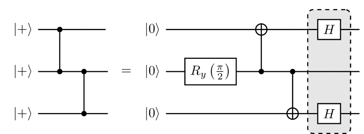
Figure 2: The circuit on the left and on the right are equal; the circuit on the left is the standard preparation of the $\ket{\mathrm{L}}_{3}$ state. The generalization to $\ket{\mathrm{L}}_{n}$ for higher (odd) $n$ follows naturally. The circuit on the right is the compiled version for the IBMQ Montreal chip. By not implementing the single-qubit gates in the grey box, the circuit depth is reduced by $25\%$. This results in a rotated linear cluster state $\ket{\psi}_{n}$ as defined in Eq.(3). This state carries the same entanglement properties as the $\ket{\mathrm{L}}_{n}$ state, and most notably can still be used to extract $\ket{\mathrm{GHZ}}$ states by adapting the measurement bases.

Implementing $\ket{\psi}_{n}$ instead of $\ket{\mathrm{L}}_{\{1,\ldots,n\}}$ allows us to reduce the circuit depth of the preparation circuit by one, when compiling for the gateset of the IBMQ Montreal device (Pauli-basis rotations, $CNOT$; see Figure 2). When considering the $\mathrm{GHZ}$ extraction, this approach has further benefits; the necessary Hadamard transformations on the first and last qubit have, in essence, been applied ‘in advance’, and the $\sigma_{x}$-measurements prescribed by the maximal pattern become $\sigma_{z}$-measurements, which are native to the device. The Pauli-based flips due to the measurement outcomes that are necessary to obtain the $\mathrm{GHZ}$ state can be performed in post-processing, as all the subsequent measurements on the $\mathrm{GHZ}$ state itself are in the Pauli basis.

To benchmark the results, we compute an estimate for the lower bound of the fidelity for both the linear cluster states and the $\mathrm{GHZ}$ states extracted from them. For the linear cluster states we use methods adapted from Tiurev and Sørensen (2022) using insights originally presented in Tóth and Gühne (2005); two measurement settings suffice to estimate the lower bound –one in which all qubits are measured in the $\sigma_{z}$-basis, and one in which all qubits are measured in the $\sigma_{x}$-basis. For the $\mathrm{GHZ}$ states we derive a similar technique. Again, two measurement settings suffice – one where all the qubits of the $\mathrm{GHZ}$ state are measured in the $\sigma_{z}$-basis, and one where all the qubits of the $\mathrm{GHZ}$ are measured in the $\sigma_{x}$-basis. Both these measurement settings are performed in parallel to the $\sigma_{z}$-measurements of the qubits not included in the $\mathrm{GHZ}$ state that are required for the extraction. All measurements are repeated $32000$ times to calculate estimates for the expectation values.

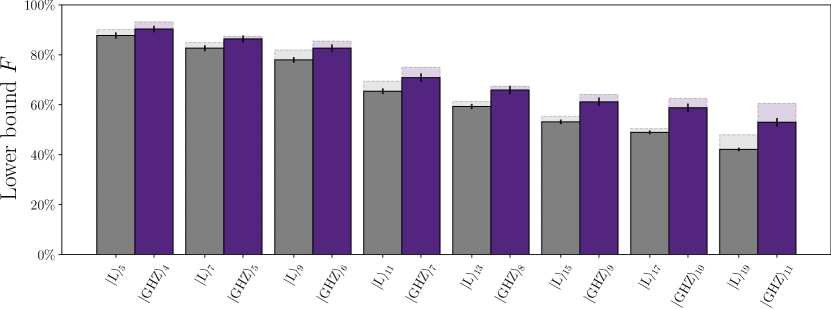
Figure 3: A lower bound of the fidelity of the rotated linear cluster and $\mathrm{GHZ}$ states prepared on the IBMQ Montreal device. We prepared rotated (see Eq. 3) linear cluster states $\ket{\psi}_{n}$ for $n\in\{5,7,\dots,19\}$ and extracted $\ket{\mathrm{GHZ}}_{m}$ states for $m\in\{4,5,\dots,11\}$using the maximal pattern introduced in Sec. III. For states with a higher number of qubits, the lower bound on the linear cluster state is increasingly worse due to a technical aspect of the estimation method (see App. C for details). The results are ordered such that each linear cluster state $\ket{\mathrm{L}}_{n}$ is paired with the $\ket{\mathrm{GHZ}}_{m}$ state extracted from it.

Figure 3 shows the lower bounds on the fidelity for all linear cluster states that we generated with the IBMQ Montreal device –as well as for the $\mathrm{GHZ}$ states we extracted from them. Note that our estimation method imposes a relative penalty for linear cluster state fidelity estimations compared to $\mathrm{GHZ}$ state fidelity estimations. However, this does not mean that the fidelity of the $\mathrm{GHZ}$ states is truly higher than that of the linear cluster states from which they were extracted: It simply means that we have used a method of bounding the fidelity from below, which works comparatively better for $\mathrm{GHZ}$ states than it does for linear cluster states. For the details of the estimation method we refer to App. C.

V Discussion

In this letter, we considered how to establish $\mathrm{GHZ}$ states between nodes that are share entanglement only with only a small number of nearest neighbours. In particular, given a linear cluster state shared between the nodes, we showed what are the possible $\mathrm{GHZ}$ states that can be obtained, the later being an indispensable resource in many quantum communication protocols including secret sharing Broadbent et al. (2009), electronic voting Xue and Zhang (2017) and anonymous conference key agreement Hahn et al. (2020).

Our results demonstrate that this process is possible but costly, since almost half of the linear cluster state qubits must be measured to obtain a $\mathrm{GHZ}$ state on the remaining qubits. Very importantly, we showed that there is in fact a tight upper bound to the size of the $\mathrm{GHZ}$ state we can obtain, higher than the one previously conjectured Briegel and Raussendorf (2001), thus solving a long-lasting open problem. We finally gave an exhaustive characterization of all possible $\mathrm{GHZ}$ states that can be extracted and provided a constructive method to obtain them, including the calculations for the necessary local rotations on the remaining qubits.

Our theoretical results are complemented by an implementation on IBM’s superconducting quantum hardware, where this near-neighbour architecture is inherent. With fidelities of $80\%$ and higher for up to nine qubits, the results show that the generation of multi-partite entangled states is possible. It is also evident from the shown results that our method of extracting $\mathrm{GHZ}$ states does not compromise the fidelity of the target states compared to the resource states, since only local operations are required. Since the generation of linear cluster states can be, depending on the specific setting, experimentally more feasible, our approach shows a potentially more robust method of generating $\mathrm{GHZ}$ states.

Finally, extending our methods to other simple graph state resources does not seem trivial and requires further research. We note, however, that deriving an analogous characterisation for ring graph states, i.e. graph states in which the leftmost and rightmost qubits of an otherwise linear cluster state are also connected, is straightforward using our methods. In this case, only a single $2$-island is possible, so the upper bound for $\absolutevalue{V_{G}{}}{}$ becomes $\lfloor\frac{n+1}{2}\rfloor$.

VI Acknowledgements

A.P., J.d.J. and F.H. acknowledge support from the German Research Foundation (DFG, Emmy Noether Grant No. 418294583) and from the European Union via the Quantum Internet Alliance project. Upon completion of this work, we became aware of work similarly motivated Mannalath and Pathak (2022); Frantzeskakis et al. (2022).

Appendix A Proof of Lemma 1

In this section we proof Lemma 1. We prove the theorem by contradiction. Fix a set $V_{G}$ such that $\{i,i+1\}\subset V_{G}{}$ and let the post-measurement state $\ket{\psi}_{V_{G}{}}$ be locally equivalent to $\ket{\mathrm{GHZ}}_{V_{G}{}}$. Assume now that there are both $j<i$ and $k>i+1$ for which both $j,k\in V_{G}{}$. W.l.o.g. assume that $j$ and $k$ are the direct left- and right neighbour of $i$ and $i+1$, respectively.

Recall that a set of generators for the linear cluster state is $\{l_{i_{0}}=\sigma_{z}^{i_{-}}\sigma_{x}^{i_{0}}\sigma_{z}^{i_{+}}\}_{i_{0}\in V_{L}}$. If the post-measurement state is locally equivalent to the $\mathrm{GHZ}$ state then there must exist a (reversible) generator transformation such that their support on $i$ and $i+1$ coincides exactly with (the generators of) the $\mathrm{GHZ}$ state - up to local Clifford rotations. We will now show that, from a reversible transformation of the $\{l_{i_{0}}\}$, it is impossible to obtain such a set of generators when $j,i,i+1,k\in V_{G}{}$. This directly implies that a measurement pattern such that the $\mathrm{GHZ}$ state can be obtained is not possible.

(A set of) generators for the $\mathrm{GHZ}$ state are, $\{\sigma_{x}^{V_{G}{}}\}\cup\{\sigma_{z}^{i_{0}}\sigma_{z}^{i_{+}}\}_{i_{0}\in V_{G}{}}$, where it is implied that $\sigma_{z}^{i_{+}}=1$ when $i_{+}\not\in V_{G}{}$. Focusing on $i$ and $i+1$, the only generators with non-trivial support are $\{\alpha,\beta,\gamma,\delta\}=\{\sigma_{a_{i}}^{i},\sigma_{a_{i}}^{i}\sigma_{a_{i+1}}^{i+1},\sigma_{a_{i+1}}^{i+1},\sigma_{b_{i}}^{i}\sigma_{b_{i+1}}^{i+1}\}$, where $a_{i},a_{i+1},b_{i},b_{i+1}\in\{x,y,z\}$ reflect the fact that the state is locally equivalent to the $\mathrm{GHZ}$ state. This implies that $a_{i}\not=b_{i}$ and $a_{i+1}\not=b_{i+1}$.

Similarly, only the generators $l_{i-1},l_{i},l_{i+1}$ and $l_{i+2}$ of the linear cluster state (i.e. those with support on $i$ or $i+1$) can have a non-trivial contribution to the generator transformation on the vertices in question. Therefore, w.l.o.g., we can focus on just these four generators and restrict our attention to vertices $i$ and $i+1$. If we show that there is no reversible transformation of $\{l_{k}\}_{k=\{i-1,i,i+1,i+2\}}$ to obtain $\{\alpha,\beta,\gamma,\delta\}$ when only considering these nodes, the lemma follows. We show there is no such transformation by exhaustive contradiction.

There are three different ways of creating generator $\alpha$: i) $\alpha\propto l_{i-1}=\sigma_{z}^{i}$, ii) $\alpha\propto l_{i}\circ l_{i+2}=\sigma_{x}^{i}$, iii) $\alpha\propto l_{i-1}\circ l_{i}\circ l_{i+2}=\sigma_{y}^{i}$, where ‘$\alpha\propto l_{i-1}$’ should be read as ‘$l_{i-1}$ takes the role of $\alpha$’, and $\circ$ denotes the (qubit-wise) product (e.g. $l_{i}\circ l_{i+1}=\sigma_{x}^{i}\sigma_{z}^{i+1}\circ\sigma_{z}^{i}\sigma_{x}^{i+1}\hat{=}\sigma_{y}^{i}\sigma_{y}^{i+1}$, where the last equality is up to an irrelevant global phase). Similarly, there are three different ways of creating generator $\gamma$: j) $\gamma\propto l_{i+2}=\sigma+{z}^{i+2}$, jj) $\gamma\propto l_{i-1}\circ l_{i+1}=\sigma_{x}^{i+2}$, jjj $\gamma\propto l_{i-1}\circ l_{i+1}\circ l_{i+2}=\sigma_{y}^{i+2}$. Picking e.g. i) and j) one sees that $\beta$ is fixed at $\propto\sigma_{z}^{i}\sigma_{z}^{i+1}$. But this is $l_{i-1}\circ l_{i+2}\propto\alpha\circ\gamma$, which would not be a reversible transformation of the generators $l_{i-1},l_{i},l_{i+1}$ and $l_{i+2}$. Any other pair from $\{\textbf{i)},\textbf{ii)},\textbf{iii)}\}$ and $\{\textbf{j)},\textbf{jj)},\textbf{jjj)}\}$ would also necessitate such a non-reversible transformation.

In essence, when viewing the generators as vectors over $\mathbf{F}^{2n}_{2}$ through the binary representation Dehaene and De Moor (2003), the argument follows from the observation that (the vector associated with) $\beta$ lies in the subspace spanned by (the vectors associated with) $\alpha$ and $\gamma$. As such there can never be a reversible (i.e. basis-preserving) operation on (the vectors associated with) $l_{i-1},l_{i},l_{i+1}$ and $l_{i+2}$ that obtains $\alpha,\beta$ and $\gamma$.

Appendix B Local-Clifford corrections to obtain $\mathrm{GHZ}$ states.

We provide a jupyter notebook for determining the required correction operations under git (2022).

Appendix C Estimation of lower bound for fidelity in the demonstrations.

We here provide details for the method of estimation of the lower bound of the fidelity of both the linear cluster state and $\mathrm{GHZ}$ state, that has been used in the demonstrational implementation. The method is presented in and adapted from Tiurev and Sørensen (2022) using insights originally presented in Tóth and Gühne (2005). The state that is prepared is

$$\ket{\psi}_{n}=\bigotimes_{i\text{ odd}}H^{i}\ket{\mathrm{L}}_{n},$$ (4)

which is a linear cluster state rotated by Clifford operations and thus a stabilizer state. Note that the generators $G^{L}$ for the stabilizer of $\ket{\psi}_{n}$ can be grouped into ‘odd’ generators $G^{L}_{o}=\{\sigma_{z}^{i-1}\sigma_{z}^{i}\sigma_{z}^{i+1}\}_{i\text{ odd}}$ and ‘even’ generators $G^{L}_{e}=\{\sigma_{x}^{i-1}\sigma_{x}^{i}\sigma_{x}^{i+1}\}_{i\text{ even}}$, where again $\sigma_{z}^{0}=\sigma_{z}^{n+1}=1$. The fidelity of the prepared state $\rho$ with the rotated linear cluster state is $F(\rho,\ket{\psi}_{n})=\tr\left[\rho\outerproduct{\psi}{\psi}_{n}\right]$. Writing $G_{o(e)}=\prod_{g\in G^{L}_{o(e)}}\frac{\mathbb{I}+g}{2}$, and using $\outerproduct{\psi}{\psi}_{n}=\prod_{g\in G}\frac{\mathbb{I}+g}{2}=G_{o}G_{e}$, we can write

$$F(\rho,\ket{\psi}_{n}) =\tr\left[G_{o}G_{e}\rho\right]$$ (5)

$$=\tr\left[G_{o}\rho\right]+\tr\left[G_{e}\rho\right]-\tr\left[\mathbb{I}\rho\right]+\tr\left[K\rho\right],$$ (6)

where $K=\left(\mathbb{I}-G_{o}\right)\left(\mathbb{I}-G_{e}\right)$. $K$ is positive semidefinite and thus we can discard the last term to obtain a lower bound for the fidelity:

$$F(\rho,\ket{\psi_{n}})\geq\mathbb{E}\left[G_{o}\right]+\mathbb{E}\left[G_{e}\right]-1,$$ (7)

where $\mathbb{E}\left[G_{o(e)}\right]=\frac{1}{2^{\absolutevalue{\mathcal{S}_{o(e)}}}}\sum_{\sigma\in\mathcal{S}_{o(e)}}\tr\left[\rho\sigma\right]$ with $\mathcal{S}_{o(e)}=\langle G^{L}_{o(e)}\rangle\subset\mathcal{S}$ the subgroup generated by the ‘odd’ (‘even’) generators of $\ket{\psi}_{n}$. Notably, all terms $\tr\left[\rho\sigma\right]$ comprise of only $\sigma_{z}$-basis ($\sigma\in\mathcal{S}_{o}$) or $\sigma_{x}$-basis ($\sigma\in\mathcal{S}_{e}$) measurements. This means that just two measurement settings suffice to estimate the lower bound: measuring all vertices in the $\sigma_{z}$-basis, and measuring all vertices in the $\sigma_{x}$-basis. By repeating these measurements $32000$ times and obtaining the outcome statistics, we estimate all terms $\tr\left[\rho\sigma\right]$ by selecting the outcomes associated with the $+1$ and $-1$ eigenspaces of all different observables.

For the $\mathrm{GHZ}$ state we use a similar method, where we now group the generators $G^{G}$ of the $\mathrm{GHZ}$ state into $G_{o}^{G}=\{\sigma_{x}^{V_{G}{}}\}$ and $G_{e}^{G}=\{\sigma_{z}^{j}\sigma_{z}^{j_{+}}\}_{j\in V_{G}{}}$, which again allows for an estimate of the lower bound with just two measurement settings. A caveat is that now there is only one ‘odd’ generator and thus $\mathbb{E}\left[G^{G}_{o}\right]=\frac{1}{2}\tr\left[\rho\mathbb{I}\right]+\frac{1}{2}\tr\left[\rho\sigma_{x}^{V_{G}{}}\right]$. By definition $\tr\left[\rho\mathbb{I}\right]=1$ and therefore the expectation value is more skewed towards $1$ than for the linear cluster state estimation. In other words it gives a higher bound on the fidelity when compared to the linear cluster state, since $G^{L}_{o}=O(2^{n})$ and as such the identity does not have such a strong impact on the estimate, especially for larger linear cluster states. To give another comparison between the two states, Figure 4 contains the same results as Figure 3 from the main text, but with the identity-term omitted. This gives a lower but more equal estimate for both classes of states.

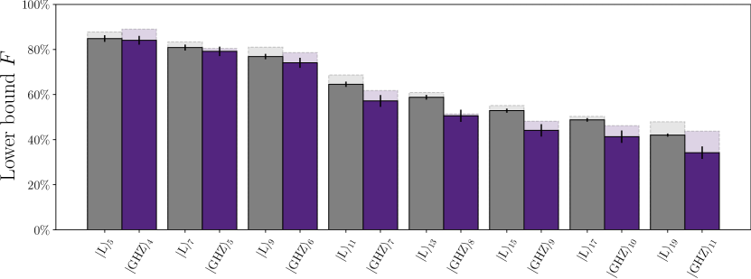
Figure 4: Lower bound on the fidelity using an adapted estimate method. In comparison with Figure 3, positive terms that favour the $\mathrm{GHZ}$ states are dropped, which renders a lower but more equal estimate on the fidelities for all states.

References

- Greenberger et al. (1989) D. M. Greenberger, M. A. Horne, and A. Zeilinger, “Going beyond bell’s theorem,” in Bell’s Theorem, Quantum Theory and Conceptions of the Universe, edited by M. Kafatos (Springer Netherlands, Dordrecht, 1989) pp. 69–72.
- Hein et al. (2006) M. Hein, W. Dür, J. Eisert, R. Raussendorf, M. V. d. Nest, and H.-J. Briegel, Entanglement in Graph States and its Applications, Tech. Rep. arXiv:quant-ph/0602096 (arXiv, 2006) arXiv:quant-ph/0602096 type: article.
- Schlingemann (2004) D.-M. Schlingemann, Journal of Mathematical Physics 45, 4322 (2004).
- Hein et al. (2004) M. Hein, J. Eisert, and H. J. Briegel, Physical Review A 69, 062311 (2004).
- Bouchet (1988) A. Bouchet, Journal of Combinatorial Theory, Series B 45, 58 (1988).
- Hahn et al. (2022) F. Hahn, A. Dahlberg, J. Eisert, and A. Pappa, Phys. Rev. A 106, L010401 (2022).
- Briegel and Raussendorf (2001) H. J. Briegel and R. Raussendorf, Physical Review Letters 86, 910 (2001).
- Van den Nest et al. (2004) M. Van den Nest, J. Dehaene, and B. De Moor, Physical Review A 69, 022316 (2004).
- Van den Nest et al. (2005) M. Van den Nest, J. Dehaene, and B. De Moor, Physical Review A 71, 062323 (2005).
- Dahlberg and Wehner (2018) A. Dahlberg and S. Wehner, Philosophical Transactions of the Royal Society A: Mathematical, Physical and Engineering Sciences 376, 20170325 (2018).
- Dahlberg et al. (2020a) A. Dahlberg, J. Helsen, and S. Wehner, Quantum Science and Technology 5, 045016 (2020a).
- Dahlberg et al. (2020b) A. Dahlberg, J. Helsen, and S. Wehner, Journal of Mathematical Physics 61, 022202 (2020b).
- Dahlberg et al. (2020c) A. Dahlberg, J. Helsen, and S. Wehner, Quantum 4, 348 (2020c).
- Christandl and Wehner (2005) M. Christandl and S. Wehner, in Advances in Cryptology - ASIACRYPT 2005, Vol. 3788, edited by D. Hutchison, T. Kanade, J. Kittler, J. M. Kleinberg, F. Mattern, J. C. Mitchell, M. Naor, O. Nierstrasz, C. Pandu Rangan, B. Steffen, M. Sudan, D. Terzopoulos, D. Tygar, M. Y. Vardi, G. Weikum, and B. Roy (Springer Berlin Heidelberg, Berlin, Heidelberg, 2005) pp. 217–235, series Title: Lecture Notes in Computer Science.
- Hillery et al. (1999) M. Hillery, V. Bužek, and A. Berthiaume, Phys. Rev. A 59, 1829 (1999).
- Broadbent et al. (2009) A. Broadbent, P.-R. Chouha, and A. Tapp, in 2009 Third International Conference on Quantum, Nano and Micro Technologies (2009) pp. 59–62.
- Murta et al. (2020) G. Murta, F. Grasselli, H. Kampermann, and D. Bruß, Advanced Quantum Technologies 3, 2000025 (2020), _eprint: https://onlinelibrary.wiley.com/doi/pdf/10.1002/qute.202000025.
- Hahn et al. (2020) F. Hahn, J. de Jong, and A. Pappa, PRX Quantum 1, 020325 (2020).
- Grasselli et al. (2022) F. Grasselli, G. Murta, J. de Jong, F. Hahn, D. Bruß, H. Kampermann, and A. Pappa, PRX Quantum 3, 040306 (2022).
- Hahn et al. (2019) F. Hahn, A. Pappa, and J. Eisert, npj Quantum Information 5, 76 (2019).
- Frantzeskakis et al. (2022) R. Frantzeskakis, C. Liu, Z. Raissi, E. Barnes, and S. E. Economou, arXiv preprint arXiv:2203.07210 (2022).
- Mannalath and Pathak (2022) V. Mannalath and A. Pathak, “Multiparty Entanglement Routing in Quantum Networks,” (2022), arXiv:2211.06690 [math-ph, physics:quant-ph].
- Gottesman (1997) D. Gottesman, “Stabilizer codes and quantum error correction,” (1997).
- Gottesman (1998) D. Gottesman, “The Heisenberg representation of quantum computers,” (1998).
- git (2022) “Supplementary information to the paper “Extracting maximal entanglement from linear cluster states”,” https://github.com/hahnfrederik/Extracting-maximal-entanglement-from-linear-cluster-states (2022), [Online; accessed 25-November-2022].
- Tiurev and Sørensen (2022) K. Tiurev and A. S. Sørensen, Phys. Rev. Research 4, 033162 (2022).
- Tóth and Gühne (2005) G. Tóth and O. Gühne, Phys. Rev. Lett. 94, 060501 (2005).
- Xue and Zhang (2017) P. Xue and X. Zhang, Scientific Reports 7, 7586 (2017).
- Dehaene and De Moor (2003) J. Dehaene and B. De Moor, Phys. Rev. A 68, 042318 (2003).