HEAT: Hardware-Efficient Automatic Tensor Decomposition for Transformer Compression

Abstract

Transformers have attained superior performance in natural language processing and computer vision. Their self-attention and feedforward layers are overparameterized, limiting inference speed and energy efficiency. Tensor decomposition is a promising technique to reduce parameter redundancy by leveraging tensor algebraic properties to express the parameters in a factorized form. Prior efforts used manual or heuristic factorization settings without hardware-aware customization, resulting in poor hardware efficiencies and large performance degradation.

In this work, we propose a hardware-aware tensor decomposition framework, dubbed HEAT, that enables efficient exploration of the exponential space of possible decompositions and automates the choice of tensorization shape and decomposition rank with hardware-aware co-optimization. We jointly investigate tensor contraction path optimizations and a fused Einsum mapping strategy to bridge the gap between theoretical benefits and real hardware efficiency improvement. Our two-stage knowledge distillation flow resolves the trainability bottleneck and thus significantly boosts the final accuracy of factorized Transformers. Overall, we experimentally show that our hardware-aware factorized BERT variants reduce the energy-delay product by $5.7\times$ with less than $1.1\%$ accuracy loss and achieve a better efficiency-accuracy Pareto frontier than hand-tuned and heuristic baselines.

1 Introduction

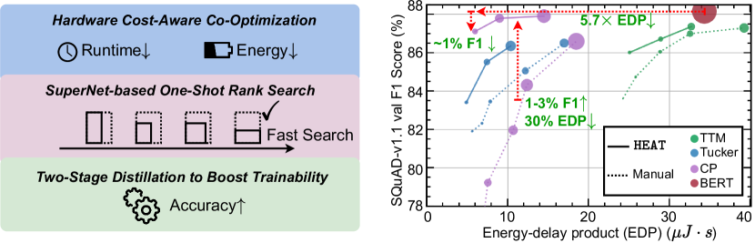
Figure 1: Hardware-efficient tensor decomposition framework HEAT achieves better accuracy-efficiency trade-off than manual settings.

Transformer models have demonstrated record-breaking performance on natural language processing (NLP) tasks (Peters et al., 2018; Devlin et al., 2019; Brown et al., 2020). However, the linear projection layers in multi-head self-attention (MHSA) and feedforward networks (FFNs) contain a large number of parameters that limit the efficient deployment of Transformers. Therefore, compressing large-scale Transformers is an essential problem in practical NLP tasks.

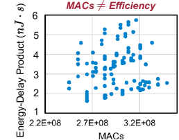
((a))

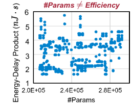
((b))

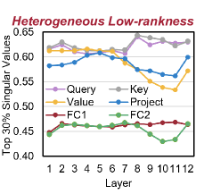
((c))

Figure 2: (a)(b) Plot different tensorization shapes and ranks in the space. Computations (MACs) and parameter counts are not accurate indicators of real hardware cost (lower energy-delay product means the application consumes less energy and runs faster (Laros III et al., 2013)). (c) Different tensors in BERT-base show different low-rankness, thus requiring per-tensor customization.

Tensor decomposition (Kolda & Bader, 2009) leverages the higher-order structure in tensors to efficiently express it in a factorized form, e.g., CP (Phan, 2011), tucker (Tucker, 1966), tensor-train (TT) (Oseledets, 2011) decomposition. It has found many applications in computer vision (Panagakis et al., 2021). Tensor factorization can be applied to matrices by first tensorizing (Anandkumar et al., 2014; Novikov et al., 2015) them (reshaping them into a higher-order tensor) and then factorizing that tensor. Among the many model compression methods (Zhen et al., 2022; Hrinchuk et al., 2020; Chen et al., 2018; Zhang et al., 2022), it is a particularly promising approach to exploring the intrinsic redundancy of NN weight matrices. Prior work has successfully applied this method to reduce the number of parameters and computations in NNs by manually selecting the tensorization shapes and ranks (Novikov et al., 2015; Sidiropoulos et al., 2017; Hrinchuk et al., 2020; Chen et al., 2018; Kossaifi et al., 2020; Deng et al., 2019; Yin et al., 2021b; Tjandra et al., 2018; Gu et al., 2021).

However, three critical issues remain unresolved. First, improvements in compression metrics do not necessarily translate to better hardware efficiency, a distinction ignored by most prior work. As shown in Fig. 2(a) and 2(b), number of multiply-accumulate operations (MACs) and parameters are imprecise indicators of energy efficiency and execution speed on real hardware. This implies that a high compression ratio may not translate to real hardware efficiency benefits. Moreover, we observe heterogeneous low-rank characteristics in different weight matrices in Fig. 2(c), but previous methods ignore this heterogeneity and manually assign a global setting to all matrices based on heuristics (Deng et al., 2019; Hrinchuk et al., 2020; Chen et al., 2018; Kossaifi et al., 2019), failing to explore the huge design space. An additional challenge of factorized Transformers is the non-trivial performance drop after tensor decomposition. Direct re-training cannot recover the accuracy of factorized Transformers due to the optimization difficulty of cascaded tensor contractions, which hinders their practical deployment.

To solve these challenges, we propose HEAT, a hardware-efficient tensor decomposition framework that features automated tensor decomposition with hardware-aware optimization, shown in Fig. 1. HEAT can efficiently explore the huge design space of tensorization while significantly improving the hardware efficiency based on the following approaches: (1) compared to prior hardware-unaware tensor decomposition work, HEAT incorporates hardware cost feedback in the tensorization optimization flow to find expressive and hardware-efficient tensorization settings; (2) instead of manually selecting a global rank setting via trial-and-error, HEAT leverages the heterogeneous low-rank property of different tensors and adopts a novel Rank SuperNet-based method to automatically search for efficient per-tensor rank settings in the exponentially large space with one-shot re-training cost; (3) HEAT resolves the trainability challenge of factorized Transformers by introducing a two-stage knowledge distillation flow to significantly boost the task performance.

Based on the approaches in HEAT, we make the following contributions:

• We deeply investigate the hardware efficiency of tensor decomposition-based model compression methods and propose an automatic framework for hardware-efficient Transformer factorization.

• We move beyond conventional compression metrics and incorporate hardware cost into optimization to find hardware-efficient tensorization settings.

• We propose a novel Rank SuperNet to explore the exponential space of heterogeneous per-tensor rank settings to push forward the accuracy-efficiency Pareto front with one-shot re-training cost.

• We discuss the trainability bottleneck of factorized Transformer and resolve it via a two-stage distillation recipe to remedy the task performance degradation from factorization.

Our searched factorized BERT models outperform the original BERT with an estimated 5.7$\times$ lower energy-delay product (EDP) and surpass hand-tuned and heuristic baselines with 25%-30% lower EDP and 1-3% accuracy improvement on SQuAD-v1.1 and SST-2 datasets.

2 HEAT Automatic Tensor Decomposition Framework

2.1 Understanding Hardware-Efficient Tensor Decomposition

Tensor Decomposition.  We first briefly introduce the basics of tensor decomposition. As shown in Fig. 3, a matrix ${\mathbf{W}}\in\mathbb{R}^{M\times N}$ is tensorized into a high-order tensor $\mathcal{X}$ and further approximated by the product or summation of a series of smaller core tensors. Representative decompositions include CP (Phan, 2011), Tucker (Tucker, 1966), and tensor-train matrix (TTM) (Oseledets, 2011). For example, the order-$d$ TTM decomposition is formulated by

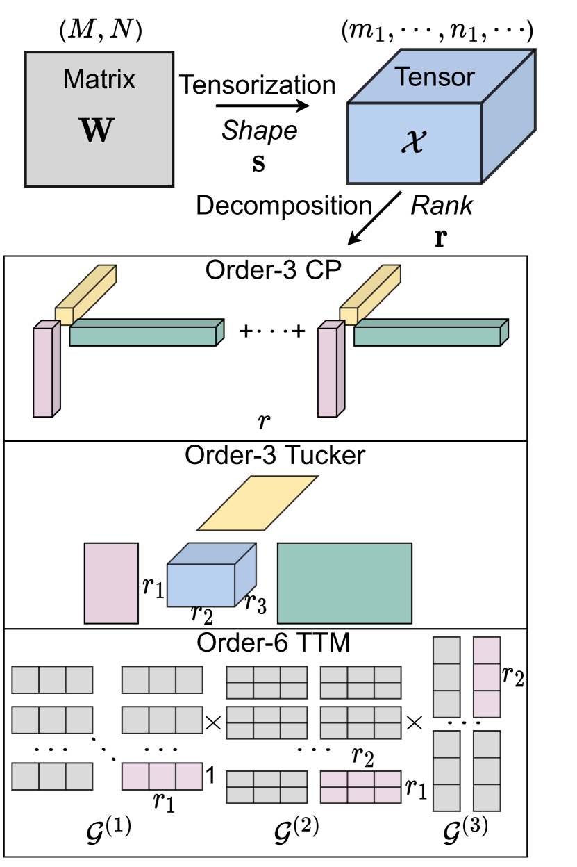
Figure 3: Illustration of tensor decomposition.

$$\mathcal{X}((i_{1}, j_{1}),\cdots\!,(i_{d},\!j_{d}))\!=\!\mathcal{G}^{(1)}\!((i_{1},j_{1}),:)\cdots\mathcal{G}^{(d)}(:,(i_{d},j_{d})),$$ (1)

where each $\mathcal{G}^{(i)}\in\mathbb{R}^{r_{i-1}\times m_{i}\times n_{i}\times r_{i}}$ is called a core tensor, the size of tensorized $\mathcal{X}$ is called tensorization shape, i.e., ${\bm{s}}=(m_{1},\cdots,n_{1},\cdots)$, where $M=\prod_{i}m_{i}$ and $N=\prod_{i}n_{i}$. The variable dimensions of cores are called decomposition ranks, i.e, ${\bm{r}}=(r_{0},r_{1},\cdots,r_{d-1},r_{d})$. The compression ratio is $c=\sum_{i}r_{i-1}m_{i}n_{i}r_{i}/MN$.

To find a hardware-efficient decomposition, the goal is to determine the tensorization shape ${\bm{s}}$ and rank ${\bm{r}}$ for each matrix ${\mathbf{W}}$ that minimizes energy-delay product while maintaining high accuracy.

Design Space.  The design space of possible (${\bm{s}}$, ${\bm{r}}$) pairs is exponentially large. We use Tucker decomposition as an example. Given an $M\times N$ matrix ${\mathbf{W}}$, we assume its candidate factorization orders are $D=(d_{1},\cdots,d_{i},\cdots,d_{k})$. For any order $d_{i}\in D$, we define $\mathcal{S}_{i}$ as all possible tensorization shapes, and we have $|\mathcal{S}_{i}|=\mathcal{O}((d_{i}!)^{2})$. For each tensorization shape ${\bm{s}}_{j}=(m_{1},\cdots,m_{d_{i}/2},n_{1},\cdots,n_{d_{i}/2})\in\mathcal{S}_{i}$, we denote the set of total possible ranks as $\mathcal{R}_{ij}$, and one example rank setting is ${\bm{r}}=(r_{1},\cdots,r_{d_{i}})\in\mathcal{R}_{ij}$. There are $\mathcal{O}(\sum_{i,j}|\mathcal{R}_{ij}|)\approx\mathcal{O}(\sum_{i}MN(d_{i}!)^{2})$ different factorization settings for this matrix. If we wish to explore per-tensor factorization settings for a DNN with $L$ weight matrices, then the complexity explodes to $\mathcal{O}(\prod_{l}^{L}(\sum_{i}M^{l}N^{l}(d_{i}!)^{2}))$. For example, the total possible decompositions for BERT-base are roughly $10^{632}$. Exploring this huge combinatorial design space via brute-force search is intractable, especially considering that it requires costly model re-training and hardware cost simulation to evaluate each factorization shape-rank pair (${\bm{s}}$, ${\bm{r}}$).

Formulation.  To make this intractable problem efficiently solvable, we formulate the search as a three-level hierarchical optimization as follows,

$$\texttt{Level 3}:~{}\text{Train factorized model:}~{}\Theta^{*}({\bm{s}}^{*},{\bm{r}}^{*})=\operatorname*{arg\,min}_{\Theta}\mathcal{L}(\Theta({\bm{s}}^{*},{\bm{r}}^{*}),\mathcal{D}_{trn}),$$ (2)

$$~{}~{}~{}\texttt{Level 2}:~{}\text{Search rank:}~{}{\bm{r}}^{*}=\operatorname*{arg\,min}_{{\bm{r}}}~{}\big{(}1-\texttt{Acc}(\Theta^{*}({\bm{s}}^{*},{\bm{r}}))\big{)}\texttt{Cost}^{*}({\bm{s}}^{*},{\bm{r}}|\alpha)^{\gamma},$$

$$\quad\quad\quad\quad\quad\quad\quad\quad\quad\quad\Theta^{*}({\bm{s}}^{*},{\bm{r}})=\operatorname*{arg\,min}_{\Theta}\mathcal{L}(\Theta({\bm{s}}^{*},{\bm{r}}),\mathcal{D}_{trn}),$$

$$~{}~{}~{}~{}~{}~{}\texttt{Level 1}:~{}\text{Search shape:}~{}{\bm{s}}^{*}=\texttt{Pareto}_{{\bm{s}}}\big{(}\texttt{Cost}^{*}({\bm{s}},{\bm{r}}|\alpha),\epsilon,c)$$

$$\epsilon=\|{\mathbf{W}}-{\mathbf{W}}^{\prime}({\bm{s}},{\bm{r}})\|_{\mathcal{F}}/\|{\mathbf{W}}\|_{\mathcal{F}},~{}\texttt{Cost}^{*}({\bm{s}},{\bm{r}}|\alpha)=\min_{m}~{}\min_{p}~{}\texttt{Cost}({\bm{s}},{\bm{r}},m,p|\alpha).$$

In Level 1, given an accelerator architecture $\alpha$, we find a Pareto optimal tensorization shape ${\bm{s}}^{*}$ that minimizes decomposition error $\epsilon$, compression ratio $c$, and the minimum hardware cost $\texttt{Cost}^{*}$ obtained by optimizing tensor contraction path ($p$) and hardware mapping ($m$). We use a standard energy-delay product (EDP) as the hardware cost to reflect both energy consumption and runtime cost. Then in Level 2, we search for optimal per-tensor rank settings ${\bm{r}}^{*}$ while minimizing hardware cost and maximizing the task-specific performance. In Level 3, we train the factorized Transformer model with the optimal (${\bm{s}}^{*}$, ${\bm{r}}^{*}$) settings to find its optimal parameters $\Theta^{*}({\bm{s}}^{*},{\bm{r}}^{*})$.

2.2 The Proposed HEAT Framework

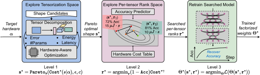
Figure 4: Overview of our hardware-efficient automatic tensor decomposition framework HEAT.

To solve this three-level optimization problem efficiently, we propose a three-stage framework HEAT, summarized in Fig. 4. In the first stage, we simulate each shape candidate on a given inference accelerator architecture $\alpha$ and build a hardware cost table for all shapes $\mathcal{T}:\mathcal{S}\times\mathcal{R}\rightarrow\texttt{Cost}$, from which we select one Pareto optimal shape ${\bm{s}}^{*}$ with low decomposition error $\epsilon$, low compression ratio $c$, and low hardware cost. All matrices with the same size share this tensorization shape. We import the optimal shape ${\bm{s}}^{*}$ to the second stage, a one-shot rank search flow that efficiently explores per-tensor rank settings with minimum model re-training cost. With the searched optimal shape and rank (${\bm{s}}^{*}$, ${\bm{r}}^{*}$), we enter the last step, a knowledge distillation-based re-training flow to recover the accuracy of factorized Transformer.

2.2.1 Level 1: Pareto Optimal Tensorization Shape Search

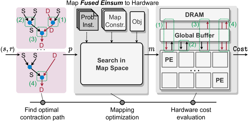
Figure 5: Efficiently map fused Einsum to Simba-L architecture aware of four memory access types.

The shape of the high-order tensor $\mathcal{X}$ is critical to the approximation error and hardware efficiency. Unlike prior work that empirically selects the tensorization shape based on heuristics, we wish to find one that can achieve low approximation error with minimal hardware cost, which corresponds to multi-objective optimization. To determine the real hardware cost of a given tensorization, as shown in Fig. 5, we must find a near-optimal contraction path $p$ and map it to the hardware $\alpha$ with an optimal mapping $m$.

Tensor Contraction Path Optimization.  A factorized linear layer requires a series of tensor contractions, which can be described by a symbolic Einsum equation, as shown in Fig. 6. The order in which these tensors are contracted, or the contraction path, is critical to hardware efficiency. For example, we show a CP factorized layer in Fig. 6. The (768$\times$768) matrix is first reshaped to an order-3 (768$\times$12$\times$64) tensor. Given a rank of 280, this tensor is decomposed into a length-280 weight vector and three CP cores. Multiplying the input $x$ with CP cores corresponds to this Einsum equation: bc,a,da,ea,ca$\rightarrow$bde. A naive tensor contraction path of this equation is shown on the left tree of Fig. 6. Each node represents a 2-operand tensor operation. Simply following the left-to-right association order leads to considerable computation and intermediate storage overhead due to the many outer product operations. In contrast, a MAC-optimal path with a more efficient association order reduces hardware cost by orders of magnitude (Smith & Gray, 2018). Note that not all nodes in the tree need to be calculated on the fly. We can pre-compute static and contracting nodes to eliminate redundant memory and computation cost, e.g., element-wise multiplication and batched inner products. Static nodes mean their inputs are known before inference, and contracting nodes mean those operations reduce the tensor size. Hence, we only need to implement the pre-computed MAC-optimal path on the hardware accelerator.

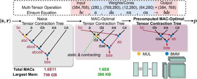
Figure 6: Our pre-computed MAC-optimal contraction path can significantly save hardware cost.

Map Fused Einsum to Hardware.  To efficiently implement factorized tensor operations, we customize our accelerator Simba-L (Shao et al., 2019) to perform a 1024-element matrix-vector multiplication each cycle to achieve high utilization on factorized Einsum workloads. However,

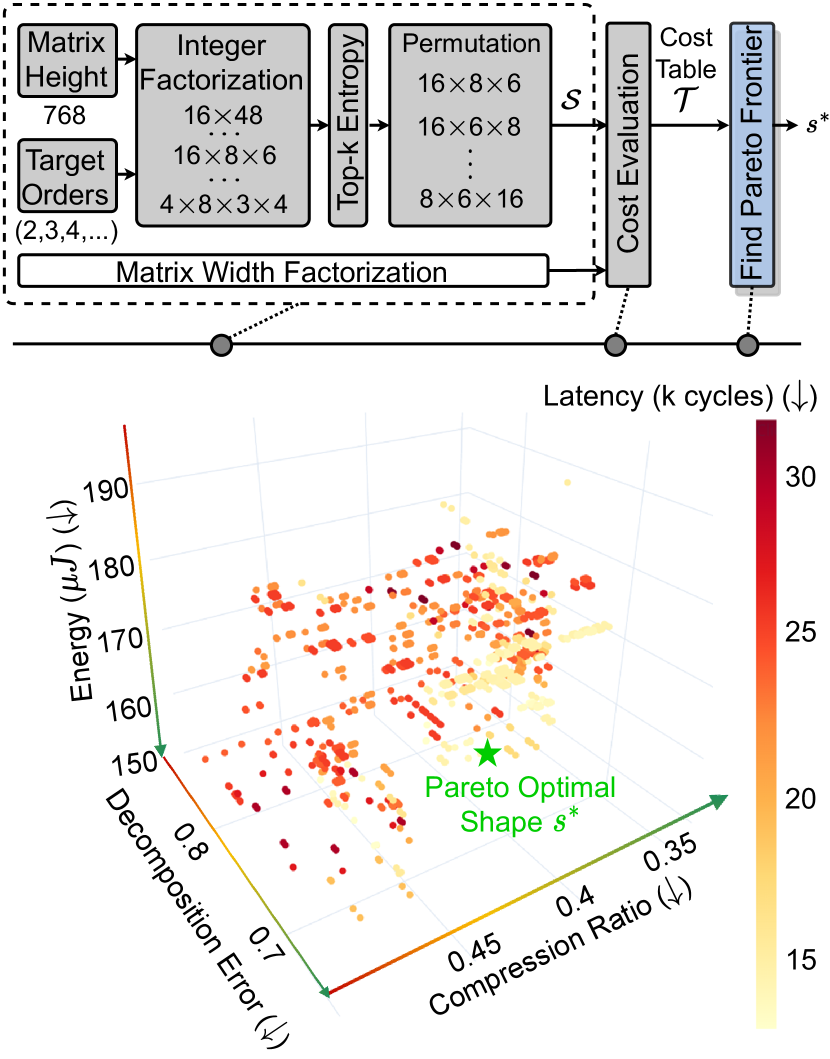
Figure 7: Top: Generate shape candidates and find the Pareto optimal shape ${\bm{s}}^{*}$ based on the cost table $\mathcal{T}$. Bottom: The Energy-Latency-Error-Ratio space with $\sim$3000 candidate shape-rank pairs.

individually implementing each 2-operand node in $p$ would realize minimal efficiency benefit since the intermediate tensors are always stored in DRAM, introducing nontrivial data movement cost. Instead, we implement a fused Einsum, minimizing redundant DRAM accesses by storing intermediate results in on-chip SRAM whenever possible to obtain the minimum hardware cost $\texttt{Cost}^{*}({\bm{s}},{\bm{r}}|\alpha)$ (See Appendix A1). We use Timeloop (Parashar et al., 2019) to search for an efficient mapping $m$ while minimizing energy-delay product, map the fused Einsum to the accelerator, and evaluate the energy and runtime.

Search for the Pareto Optimal Shape: ${\bm{s}}^{*}$.  We construct a search space for shape candidates. In Fig. 7, we perform integer factorization on the matrix height/width, select top-k shapes with maximum entropy since we prefer uniform shapes across axes, and permute the axes to form the shape candidates $\mathcal{S}$. Then we decompose the matrix with all shape candidates to get the approximation error and evaluate their hardware costs to form a cost table $\mathcal{T}$ (See details in Appendix A2). We visualize the cost table in Fig. 7. We automatically detect the points on the Pareto-optimal surface and heuristically select the best shape ${\bm{s}}^{*}$ with the lowest decomposition error. We repeat this process for all different sizes of matrices in the model, completing the Level 1 optimization.

2.2.2 Level 2: Weight-Sharing Per-Tensor Rank Optimization

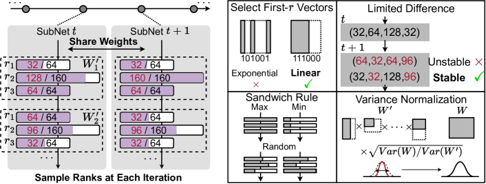
Figure 8: Left: Rank SuperNet training flow. Right: Illustration of training stabilization techniques.

One-Shot Rank Search via Weight-Sharing SuperNet.  The challenges in the Level 2 optimization are twofold: (1) the exponentially large per-tensor rank search space and (2) the prohibitive cost of accuracy evaluation on a shape-rank pair. These barriers make it impossible to select the best rank by enumeration. Inspired by the high efficiency in weight-sharing neural architecture search (NAS) (Wu et al., 2019; Cai et al., 2020), we propose a Rank SuperNet where each SubNet corresponds to a per-tensor rank setting. As shown in Fig. 8, at each iteration, we randomly sample valid ranks for each tensor, and different SubNets share the same set of parameters. Hence, we can efficiently explore a large space of different rank settings. Training this SuperNet can easily suffer from instability issues due to a large rank sampling variance, so we adopt four techniques to stabilize the SuperNet convergence. (1) We only sample the first $r$ vectors along each axis to reduce the search space. (2) We limit the rank difference across iterations to reduce variance. (3) We adopt sandwich rules (Yu & Huang, 2019) to train the largest, smallest, and randomly sampled SubNets together. (4) We normalize the reconstructed matrix ${\mathbf{W}}^{\prime}({\bm{s}},{\bm{r}})$ with a scaling factor $\sqrt{Var({\mathbf{W}})/Var({\mathbf{W}}^{\prime})}$ to match the target variance of ${\mathbf{W}}$ and avoid statistical instability.

Per-Tensor Rank Selection via Evolutionary Search: ${\bm{r}}^{*}$.  We randomly sample 2,560 SubNets

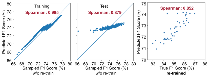
Figure 9: Left, Middle: Our accuracy predictor shows high prediction fidelity and generalization on BERT-base SQuADv-1.1. Right: Predicted F1 is an accurate proxy of the ground-truth re-trained F1.

from the Rank SuperNet and train a random forest $\mathcal{P}:({\bm{s}},{\bm{r}})\rightarrow\texttt{Acc}$ to predict the validation accuracy based on the factorization settings, which is a fast proxy to reduce validation cost. In Fig. 9, we observe a high fidelity (high Spearman correlation) between the predicted and the re-trained F1. In addition to accuracy maximization, network hardware cost must also be considered. The total energy $E_{tot}$ and runtime $T_{tot}$ of the model is simply the sum of all layer costs. We use evolutionary search to find the optimized factorization settings: $\min_{{\bm{r}}}~{}(1-\texttt{Acc})(E_{tot}\cdot T_{tot})^{\gamma}$, where $\gamma$ is empirically set to 0.25.

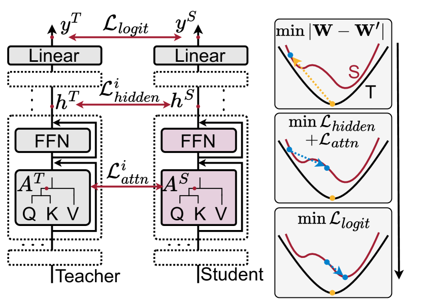
Figure 10: Layer-wise and logit distillation for factorized Transformers.

2.2.3 Level 3: Trainability Boost with Two-stage Distillation

Since decomposition errors will accumulate through layers, re-training is necessary to recover accuracy. However, optimization of factorized tensors is difficult, making trainability a bottleneck for factorized Transformers. To solve this issue, we propose a two-stage distillation flow. First, we perform optimal layer-wise projection to find the tensor decomposition that minimizes matrix approximation error, $\min_{{\mathbf{W}}_{i}^{\prime}}\sum_{i}\|{\mathbf{W}}_{i}-{\mathbf{W}}^{\prime}_{i}\|_{\mathcal{F}}$. Then we distill the layer-wise knowledge from the teacher $T$ to the factorized student $S$ both on the attention maps $A$ and hidden states $h$ on each Transformer block.

$$\mathcal{L}_{attn}+\mathcal{L}_{hidden}=\sum_{i}\mathcal{L}_{attn}^{i}+\mathcal{L}_{hidden}^{i}$$ (3)

$$=\sum_{i}\texttt{CosEmbed}(A^{S}_{i},A^{T}_{i})+\texttt{CosEmbed}(h^{S}_{i},h^{T}_{i})$$

After the layer-wise alignment, we only apply last-layer logit distillation to provide more optimization freedom for the student,

$$\centering\mathcal{L}_{logit}=\frac{1}{2}\mathcal{L}_{KL}(y^{S}/\tau,y^{T}/\tau)+\frac{1}{2}\mathcal{L}_{CE}(y^{S},y^{T}).\@add@centering$$ (4)

3 Results

3.1 Experiment setup

Datasets, Models, and Training Settings.  We search the decomposition settings on BERT-base/DistilBERT with the question-and-answer dataset SQuAD-v1.1 and evaluate on SQuAD and SST-2 datasets. We use the original model fine-tuned on SQuAD as the teacher model. We searched 3 variants, from HEAT-a1 to HEAT-a3, with different energy-delay product (EDP) to cover different design points. Breakdown on the compression ratio, runtime, and energy cost of HEAT variants are in Appendix A13 and A14. We evaluate three representative tensor decomposition methods: TTM, Tucker, and CP. We follow the standard BERT fine-tuning settings. Please see Appendix A3, A4, and A5 for detailed settings of the SuperNet training, evolutionary search, and knowledge distillation.

Hardware Settings. We use Timeloop (Parashar et al., 2019) as the mapper and hardware cost simulator, with energy models based on 5nm technology. Detailed architecture configurations of our customized Simba-L accelerator and simulation settings can be found in Appendix A2.

3.2 Main Results

Results on BERT-base SQuAD.v1-1.  We compare our searched factorization settings with (1) the original fine-tuned BERT, (2) SR-Manual: manually-selected shape and rank settings, and (3) S(Ours)-R(TensorLy): searched optimal tensorization shapes and heuristic ranks by TensorLy (Kossaifi et al., 2019) based on the target compression ratio. In Table 1 and Fig. 12, HEAT achieves the best performance-efficiency Pareto front, surpassing manual and heuristic tensor decomposition baselines.

With TTM decomposition, HEAT improves the F1 score by +0.65% with 8% fewer parameters and 8.8% lower hardware cost on average. The compact HEAT-a1 benefits the most from our heterogeneous per-tensor rank settings and significantly outperforms manual and heuristic decomposition with +1.6% higher F1 scores. However, compared to the original BERT, we note that TTM-factorized BERT is not very hardware-efficient, as the TTM optimal contraction path reconstructs the weight matrix and performs the standard linear operation.

	TTM			Tucker			CP
Model	#Params (M)$\downarrow$	F1 (%)$\uparrow$	EDP ($\mu J\cdot s$)$\downarrow$	#Params (M)$\downarrow$	F1 (%)$\uparrow$	EDP ($\mu J\cdot s$)$\downarrow$	#Params (M)$\downarrow$	F1 (%)$\uparrow$	EDP ($\mu J\cdot s$)$\downarrow$
BERT-base	109.50	88.16	34.31	109.50	88.16	34.31	109.50	88.16	34.31
SR-Manual-1	35.04	83.60	24.27	38.10	81.90	5.63	43.13	68.95	4.48
SR-Manual-2	38.71	84.74	25.86	39.71	82.31	6.85	54.27	79.22	7.57
S(Ours)-R(TensorLy)-1	36.15	83.89	24.42	35.81	80.43	4.06	46.38	85.81	5.45
S(Ours)-R(TensorLy)-2	39.78	85.49	27.18	39.48	82.00	4.93	55.52	87.21	9.37
HEAT-a1	41.60	86.01	25.06	42.14	83.41	4.91	48.88	87.11	5.99
SR-Manual-3	42.37	86.05	28.87	42.64	83.45	7.87	60.88	81.96	10.70
S(Ours)-R(TensorLy)-3	43.33	85.84	29.05	42.63	82.96	5.66	60.31	87.74	9.62
HEAT-a2	46.42	86.71	28.93	50.96	85.51	7.45	59.08	87.79	9.01
SR-Manual-4	50.90	86.99	32.57	52.94	85.05	12.21	69.12	84.31	12.40
SR-Manual-5	60.68	87.29	39.25	59.17	86.50	17.00	83.98	86.59	18.50
S(Ours)-R(TensorLy)-4	51.76	86.64	33.55	51.87	85.19	9.27	68.79	87.62	14.40
S(Ours)-R(TensorLy)-5	61.45	87.74	49.27	62.26	86.76	11.90	82.43	88.14	18.00
HEAT-a3	54.68	87.36	32.72	63.62	86.35	10.40	74.15	87.91	14.50
Avg. Improv.	-8.15%	+0.65	-8.80%	+0.09%	+1.03	-30.28%	-9.07%	+3.45	-25.30%

Table 1: Compare our HEAT-series with baseline decomposition methods on BERT-base SQuAD-v1.1 in terms of #Params, F1 score, and energy-delay product (EDP) across three decomposition methods.

With Tucker decomposition, HEAT-series boosts the F1 score by +1.03 with +30% higher efficiency than handcrafted settings that typically reshape the matrix to a high-order tensor (e.g., order 6 or 8) (Yin et al., 2021b; Tjandra et al., 2018). However, this widely-used heuristic turns out to be much less efficient than the lower-order tensorization found by HEAT, because the high-order Einsum equation includes many 2-operand Einsums with tiny tensor dimensions ($\ll$32), resulting in low hardware utilization. Though the accuracy per parameter of Tucker is slightly lower than TTM, its accuracy-to-EDP ratio is 3-5$\times$ higher than TTM.

CP decomposition is usually disfavored due to unstable optimization (de Silva & Lim, 2008), which is also evidenced by manual CP decomposition. In contrast, our search framework finds an efficient CP tensorization shape and is able to recover accuracy through re-training. HEAT-series overall can boost the F1 score by +3.45% with 25.3% less hardware cost. Compared to the original BERT, our searched HEAT-a1 can maintain accuracy ($\leq$1% drop) with 5.7$\times$ higher hardware efficiency.

Model	TTM		Tucker		CP
	F1 (%)$\uparrow$	EDP$\downarrow$	F1(%)	EDP$\downarrow$	F1 (%)$\uparrow$	EDP$\downarrow$
BERT-base	91.74	5.21	91.74	5.21	91.74	5.21
HEAT-a1	90.02	4.24	87.27	0.45	91.40	0.50
HEAT-a2	90.90	5.65	88.42	0.69	91.51	0.79
HEAT-a3	91.20	7.34	89.91	1.02	91.17	1.34

tableEvaluation of HEAT on SST-2 with decomposition settings searched on SQuAD-v1.1.

Results on BERT-base SST-2.  We re-train HEAT-variants on SST-2 to evaluate the generalization of the decomposition settings searched on SQuAD. In Table 3.2, we observe that when adapted to a new downstream task with a smaller sequence length (128), our searched Tucker and CP factorization can still largely maintain the F1 score with 4-10$\times$ higher hardware efficiency.

Results on DistilBERT SQuADv-1.1 and SST-2.  Our tensor decomposition method can be applied to compact Transformers as an orthogonal compression technique. Based on DistilBERT (Sanh et al., 2019), a 6-layer compact version of BERT-base, we searched three HEAT-variants in Table 2. Our HEAT-series can achieve comparable F1 scores with 5.7$\times$ higher efficiency on SQuAD-v1.1. On SST-2, HEAT-series can maintain the accuracy while saving 3-10$\times$ hardware cost.

	SQuADv1.1						SST-2
	TTM		Tucker		CP		TTM		Tucker		CP
	F1$\uparrow$	EDP$\downarrow$	F1$\uparrow$	EDP$\downarrow$	F1$\uparrow$	EDP$\downarrow$	Acc$\uparrow$	EDP$\downarrow$	Acc$\uparrow$	EDP$\downarrow$	Acc$\uparrow$	EDP$\downarrow$
DistilBERT	86.90	8.58	86.90	8.58	86.90	8.58	91.97	1.30	91.97	1.30	91.97	1.30
HEAT-a1	85.26	6.71	83.66	1.72	87.09	1.50	91.40	1.23	90.30	0.17	91.28	0.13
HEAT-a2	86.42	7.76	85.21	2.56	87.89	2.26	90.60	1.64	91.30	0.23	91.06	0.20
HEAT-a3	86.92	8.74	86.15	3.21	88.18	3.63	90.60	2.10	90.60	0.29	91.63	0.34

Table 2: Compare three HEAT-variants with DistilBERT-base on SQuAD-v1.1 and SST-2 datasets.

3.3 Discussions

Ablation on SuperNet Training Techniques.  We perform ablation studies on the Rank SuperNet

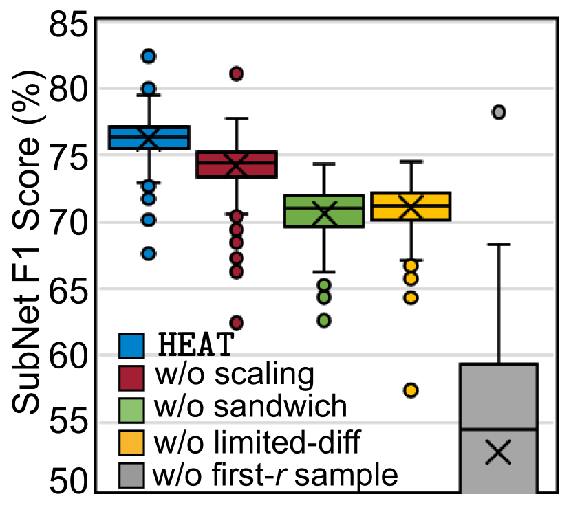
Figure 11: Ablation on SuperNet training.

training techniques in Fig. 11. We individually remove one technique at a time and show the F1 score distribution of 1,024 SubNets. With all training techniques, our HEAT framework achieves the best SuperNet convergence with the highest SubNet F1 scores.

Evolution vs. Random Rank Settings.  In Fig. 12, we further fine-tune 40 SubNets on SQuAD-v1.1 with our searched tensorization shape and randomly sampled per-tensor ranks, denoted as S(Ours)-R(Random). We can observe that (1) even with random ranks, our searched shape can still outperform manually selected shapes; (2) and the evolutionary search effectively explores the Pareto front of the rank distribution.

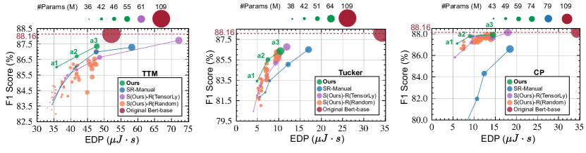
Figure 12: Comparison of our searched factorization with baselines in the accuracy vs. EDP space on BERT-base SQuAD-v1.1.

Ablation on Re-Training Recipes.  We compare different re-training methods in Table 3 and visualize four representative attention maps, which are key indicators of the model representability. Direct re-training with cross-entropy loss suffers from severe performance loss due to optimization difficulty, and the attention map can barely be recovered. One-stage distillation is not effective since the layer-wise loss is not compatible with logit distillation loss, especially in the later optimization stage. When we decouple layer-wise and logit distillation, especially when attention and hidden state distillation are combined in the first stage, we observe significant improvement in accuracy. The abundant patterns in the visualized attention maps are mostly recovered.

	BERT-base	w/o KD	One-Stage KD				Two-Stage KD
		Finetune (16)	L (16)	A+L (16)	H+L (16)	A+H+L (16)	A(8) $\rightarrow$ L(8)	H(8) $\rightarrow$ L(8)	A+H(8) $\rightarrow$ L(8)
Attention Map
F1 (%)	88.16	79.11	79.22	78.32	75.89	81.15	85.99	73.22	87.36

Table 3: Compare different re-training recipes of TTM-factorized HEAT-a3 on SQuAD-v1.1. All methods are trained for 16 epochs in total.

4 Related Work

Compression with Tensor Decomposition.  In the literature on Transformer compression, tensor decomposition is applied to compress the embedding layers (Hrinchuk et al., 2020; Chen et al., 2018; Yin et al., 2021a). However, we do not decompose the embedding matrix due to limited hardware efficiency benefits (See Appendix A7). Multi-linear attention (Ma et al., 2019) was proposed based on block-term tensor decomposition to achieve parameter-efficient Transformer. TIE (Deng et al., 2019) applied TT format to all linear matrices and proposed a new hardware design to minimize redundant computations. Recently, hybrid compression approaches have achieved strong results in Transformer compression. Low-rank decomposition was applied with weight pruning (Liu et al., 2021) or quantization to slim down BERT by 7.5$\times$. Our work delves deeply into tensor decomposition, and the proposed HEAT framework can be jointly applied with other orthogonal methods, which is one promising future direction.

Optimization of Factorized NNs.  Knowledge distillation was used to transfer the expressivity from a pre-trained teacher Transformer to the compact student model (Liu et al., 2021; Sanh et al., 2019). Bayesian tensorized NNs are put forward to automatically determine the rank in low-rank decomposition without manual settings (Hawkins et al., 2020). Our search framework is more scalable than the Bayesian method and considers the real accuracy and hardware cost instead of just matrix decomposition error and compression ratios.

5 Conclusion

In this work, we explore the large design space of hardware-efficient tensor decomposition and present HEAT, an automatic decomposition framework for Transformer model compression. We move beyond conventional manual factorization focusing only on compression ratios or computations. We consider hardware cost in the optimization loop and efficiently find expressive and hardware-efficient tensorization shapes. Our SuperNet-based one-shot rank search flow can efficiently generate optimized per-tensor decomposition rank settings. We employ a two-stage distillation flow to solve the trainability bottleneck of factorized Transformers and significantly boost their task performance. Experiments show that HEAT reduces up to 5.7$\times$ energy-delay product on our customized accelerator with less than 1.1% accuracy drop. Compared to manual and heuristic tensor decomposition methods, our searched HEAT-variants show 1-3% higher accuracy with $\sim$30% less hardware cost on average.

Appendix A1 Memory Access Types for Fused Einsum

To implement fused einsum, we separate all nodes in the tensor contraction path $p$ into 4 categories according to their memory access types, as shown in Fig. 5.

• Type 1: Load dynamic (D) input from DRAM and static (S) weights from the global buffer (GB), and write the intermediate tensor back to GB for data reuse.

• Type 2: Only read/write from/to GB without costly DRAM transaction.

• Type 3: Load both operands from GB and write the final results back to DRAM.

• Type 4: Load one dynamic input from DRAM and write the final results to DRAM.

Different node types are simulated with corresponding memory access constraints in Timeloop, so we can implement a fused einsum without unnecessary DRAM access.

Appendix A2 Hardware Cost Simulation Settings

To construct the hardware cost table $\mathcal{T}$, we construct the tensorization shape candidate spaces in Table A4. For each shape, we collect all candidate ranks that are multiples of 32 or 8 and satisfy the compression ratio constraints. We use Timeloop with TSMC 5 nm energy model to simulate the fused einsum operation corresponding to each shape-rank pair. Our Simba-L architecture has a 2.91 MB global buffer and 32 PEs. Each PE has 32 32-KB weight buffers, one 64-KB input buffer, 32 384-B accumulation buffers, and 1024 8-bit MAC units. The hardware mapping objective of Timeloop-mapper is to minimize the energy-delay product. Based on the simulated hardware cost table $\mathcal{T}$, we use the paretoset library to automatically select the Pareto optimal tensorization shape for the subsequent rank search flow.

Table A4: Tensorization shape search space for the query, value, key, and projection weight matrices with three factorization methods.

Model	Candidate orders	Top-k Candidate shapes	Candidate ranks	Compression Ratio Limits	#Candidates
TTM	6, 8, 10	3	Multiple of 32	0.35$\sim$0.5	3235
Tucker	4, 6, 8	3	Multiple of 8	0.35$\sim$0.5	4754
CP	2, 3	3	Multiple of 32	0.35$\sim$0.5	44

Appendix A3 Rank SuperNet Training Settings

With the searched optimal tensorization shape ${\bm{s}}^{*}$, we construct a Rank SuperNet with maximum ranks following a $\sim$60% target compression ratio. We use the original fine-tuned BERT-base as the teacher model and launch the 10-epoch logit distillation flow to train the Rank SuperNet. We use Adam optimizer with a learning rate of 3e-5 and a linear decay schedule. In the limited difference technique, we restrict the maximum allowed rank change across iterations to 3. We use a sandwich rule with one largest SubNet, one smallest SubNet, and two randomly sampled SubNets.

Appendix A4 Per-tensor Rank Search Settings

With the trained Rank SuperNet, we uniformly sample 2560 SubNets with the largest and smallest SubNets and evaluate their validation F1 scores on a 5% validation set. We use 95% SubNet evaluation data to train a random forest ensemble model as the accuracy predictor. The model is an AdaBoostRegressor with 100 ExtraTreeRegressor, each tree regressor containing 60 decision trees with a maximum depth of 10.

In the evolutionary search stage, we use 200 populations with 40 parents, 80 mutations with 50% mutation probability, and 80 crossovers. After 100 steps, we obtain the optimal per-tensor rank settings.

Appendix A5 Knowledge Distillation Settings

We use a two-stage knowledge distillation flow to train the model with the searched (${\bm{s}}^{*}$, ${\bm{r}}^{*}$) settings. We use the original BERT-base as the teacher model. We first launch an 8-epoch layer-wise distillation flow with attention and hidden state mapping with a constant learning rate of 3e-5 for TTM and Tucker, 1e-5 for CP. Then, we launch an 8-epoch logit distillation flow with an initial learning rate of 1e-5 on SQuAD-v1.1 and 6e-6 on SST-2 and a linear decay rate with 10% warm-up.

Appendix A6 Breakdown of Searched HEAT Variants

Compression Ratio.  We plot the compression ratio breakdown of our searched HEAT-variants in Fig. A13. We can observe that deeper layers tend to have higher redundancy and thus have fewer parameters. Feedforward networks tend to have a lower compression ratio (fewer parameters) than query/value/key matrices.

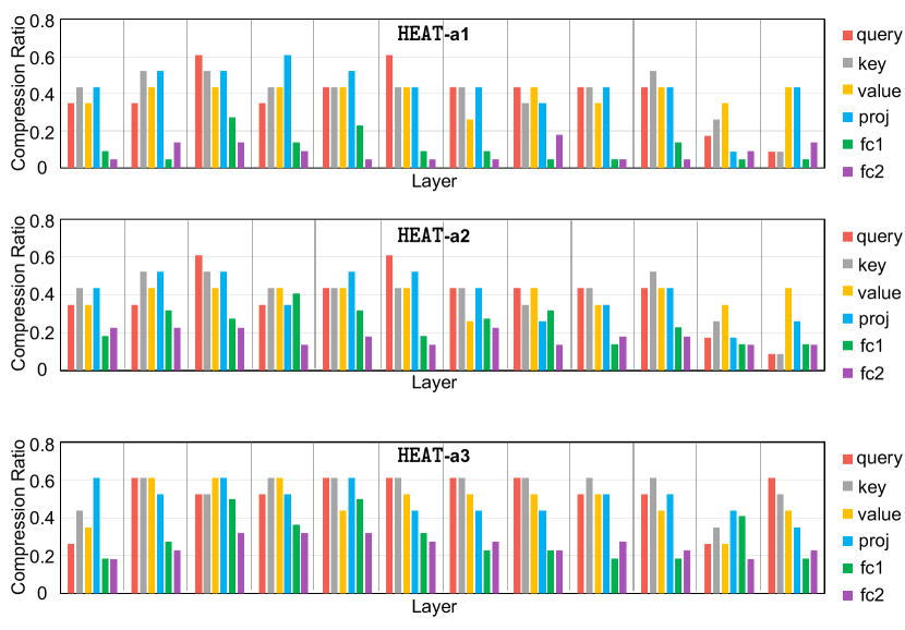
Figure A13: Compression ratio breakdown on each matrix in our HEAT-variants with TTM decomposition.

Latency and Energy.  In Fig. A14, the fully-connected (FC) layers in FFNs have lower compression ratios but nearly 4$\times$ higher latency than other linear layers. The batched matrix multiplication (BMM) in attention operations, i.e., $\mathbf{Q}\mathbf{K}^{T}$ and $\mathbf{AV}$, only take around 5.3% total latency and 19.5% total energy in the entire network, which validates that the most costly operations in Transformer are indeed linear layers.

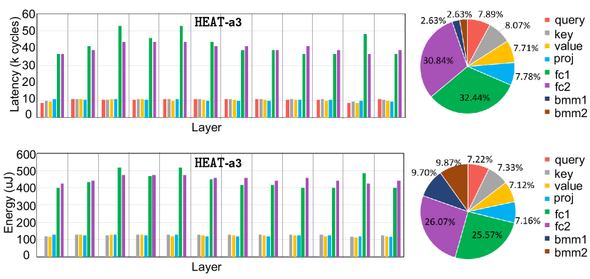
Figure A14: Latency (Top) and energy (Bottom) breakdown of HEAT-a3.

Appendix A7 Decomposition on Embedding Layers

Some prior work applies low-rank decomposition on the embedding layer in Transformer models and claims it can save parameters. However, when off-chip DRAM capacity is not a limiting factor, this embedding layer decomposition comes with a non-trivial accuracy drop and no hardware efficiency benefits. Indexing the original look-up table only contains DRAM read without extra computations. In contrast, indexing factorized tensors is very costly and requires tensor dot-product among all decomposed core tensors. The computation overhead far outweighs the saved storage capacity. Therefore, we do not decompose the embedding layers.

References

- Anandkumar et al. (2014) Animashree Anandkumar et al. Tensor decompositions for learning latent variable models. Journal of Machine Learning Research, 2014.
- Brown et al. (2020) Tom Brown, Benjamin Mann, Nick Ryder, Melanie Subbiah, et al. Language models are few-shot learners. In Proc. NeurIPS, volume 33, pp. 1877–1901, 2020.
- Cai et al. (2020) Han Cai, Chuang Gan, and Song Han. Once for all: Train one network and specialize it for efficient deployment. In Proc. ICLR, 2020.
- Chen et al. (2018) Patrick H. Chen, Si Si, Yang Li, et al. GroupReduce: Block-Wise Low-Rank Approximation for Neural Language Model Shrinking. In Proc. NeurIPS, 2018.
- de Silva & Lim (2008) Vin de Silva and Lek-Heng Lim. Tensor rank and the ill-posedness of the best low-rank approximation problem. SIAM Journal on Matrix Analysis and Applications, pp. 1084–1127, 2008.
- Deng et al. (2019) Chunhua Deng, Fangxuan Sun, Xuehai Qian, et al. TIE: Energy-efficient Tensor Train-based Inference Engine for Deep Neural Network. In Proc. ISCA, 2019.
- Devlin et al. (2019) Jacob Devlin, Ming-Wei Chang, Kenton Lee, and Kristina Toutanova. BERT: pre-training of deep bidirectional transformers for language understanding. In NAACL, pp. 4171–4186, 2019.
- Gu et al. (2021) Jiaqi Gu, Hanqing Zhu, Chenghao Feng, Mingjie Liu, Zixuan Jiang, Ray T. Chen, and David Z. Pan. Towards memory-efficient neural networks via multi-level in situ generation. In Proc. ICCV, pp. 5229–5238, October 2021.
- Hawkins et al. (2020) Cole Hawkins, Xing Liu, and Zheng Zhang. Towards Compact Neural Networks via End-to-End Training: A Bayesian Tensor Approach with Automatic Rank Determination. SIAM, 2020.
- Hrinchuk et al. (2020) Oleksii Hrinchuk, Valentin Khrulkov, Leyla Mirvakhabova, et al. Tensorized Embedding Layers. In Proc. EMNLP, 2020.
- Kolda & Bader (2009) Tamara G Kolda and Brett W Bader. Tensor decompositions and applications. SIAM Rev., 51(3):455–500, 2009.
- Kossaifi et al. (2019) Jean Kossaifi, Yannis Panagakis, Anima Anandkumar, and Maja Pantic. Tensorly: Tensor learning in python. Journal of Machine Learning Research, 20(26):1–6, 2019.
- Kossaifi et al. (2020) Jean Kossaifi, Zachary C. Lipton, Arinbjörn Kolbeinsson, Aran Khanna, Tommaso Furlanello, and Anima Anandkumar. Tensor regression networks. J. Mach. Learn. Res., 21(1), 2020.
- Laros III et al. (2013) James H. Laros III, Kevin Pedretti, Suzanne M. Kelly, Wei Shu, Kurt Ferreira, John Vandyke, and Courtenay Vaughan. Energy Delay Product, pp. 51–55. Springer London, 2013. ISBN 978-1-4471-4492-2. doi: 10.1007/978-1-4471-4492-2_8. URL https://doi.org/10.1007/978-1-4471-4492-2_8.
- Liu et al. (2021) Yuanxin Liu, Zheng Lin, and Fengcheng Yuan. ROSITA: Refined BERT cOmpreSsion with InTegrAted techniques. In Proc. AAAI, 2021.
- Ma et al. (2019) Xindian Ma, Peng Zhang, Shuai Zhang, et al. A Tensorized Transformer for Language Modeling. In Proc. NeurIPS, 2019.
- Novikov et al. (2015) Alexander Novikov, Dmitry Podoprikhin, Anton Osokin, , and Dmitry Vetrov. Tensorizing neural networks. In Proc. NIPS, 2015.
- Oseledets (2011) Ivan V Oseledets. Tensor-train decomposition. SIAM, 2011.
- Panagakis et al. (2021) Yannis Panagakis, Jean Kossaifi, Grigorios G Chrysos, James Oldfield, Mihalis A Nicolaou, Anima Anandkumar, and Stefanos Zafeiriou. Tensor methods in computer vision and deep learning. Proceedings of the IEEE, 109(5):863–890, 2021.
- Parashar et al. (2019) Angshuman Parashar, Priyanka Raina, Yakun Sophia Shao, Yu-Hsin Chen, Victor A. Ying, Anurag Mukkara, Rangharajan Venkatesan, Brucek Khailany, Stephen W. Keckler, and Joel Emer. Timeloop: A systematic approach to dnn accelerator evaluation. In Proc. ISPASS, pp. 304–315, 2019.
- Peters et al. (2018) Matthew E. Peters, Mark Neumann, Mohit Iyyer, Matt Gardner, Christopher Clark, Kenton Lee, and Luke Zettlemoyer. Deep contextualized word representations. In NAACL, 2018.
- Phan (2011) A.H. NFEA Phan. Nfea: Tensor toolbox for feature extraction and applications. Technical Report, 2011.
- Sanh et al. (2019) Victor Sanh, Lysandre Debut, Julien Chaumond, et al. DistilBERT, a distilled version of BERT: smaller, faster, cheaper and lighter. In Proc. NeurIPS, 2019.
- Shao et al. (2019) Yakun Sophia Shao, Jason Clemons, Rangharajan Venkatesan, Brian Zimmer, Matthew Fojtik, Nan Jiang, Ben Keller, Alicia Klinefelter, Nathaniel Pinckney, Priyanka Raina, Stephen G. Tell, Yanqing Zhang, William J. Dally, Joel Emer, C. Thomas Gray, Brucek Khailany, and Stephen W. Keckler. Simba: Scaling deep-learning inference with multi-chip-module-based architecture. In Proc. MICRO, pp. 14–27, 2019.
- Sidiropoulos et al. (2017) Nicholas D. Sidiropoulos, Lieven De Lathauwer, Xiao Fu, Kejun Huang, Evangelos E. Papalexakis, and Christos Faloutsos. Tensor decomposition for signal processing and machine learning. IEEE Trans. on Signal Processing, 65(13):3551–3582, 2017.
- Smith & Gray (2018) Daniel G. A. Smith and Johnnie Gray. opt_einsum - a python package for optimizing contraction order for einsum-like expressions. Journal of Open Source Software, 3(26):753, 2018.
- Tjandra et al. (2018) Andros Tjandra, Sakriani Sakti, and Satoshi Nakamura. Tensor decomposition for compressing recurrent neural network. In Proc. IJCNN, 2018.
- Tucker (1966) L.R. Tucker. Some mathematical notes on three-mode factor analysis. Psychometrika, 1966.
- Wu et al. (2019) Bichen Wu, Xiaoliang Dai, Peizhao Zhang, Yanghan Wang, Fei Sun, Yiming Wu, Yuandong Tian, et al. FBNet: Hardware-aware Efficient Convnet Design via Differentiable Neural Architecture Search. In Proc. CVPR, 2019.
- Yin et al. (2021a) Chunxing Yin, Bilge Acun, Carole-Jean Wu, and Xing Liu. Tt-rec: Tensor train compression for deep learning recommendation models. In Proc. ICCV, 2021a.
- Yin et al. (2021b) Miao Yin, Siyu Liao, Xiao-Yang Liu, Xiaodong Wang, and Bo Yuan. Towards extremely compact rnns for video recognition with fully decomposed hierarchical tucker structure. In Proc. CVPR, 2021b.
- Yu & Huang (2019) Jiahui Yu and Thomas S. Huang. Universally slimmable networks and improved training techniques. In Proc. ICCV, 2019.
- Zhang et al. (2022) Jinnian Zhang, Houwen Peng, Kan Wu, et al. MiniViT: Compressing Vision Transformers with Weight Multiplexing. In Proc. CVPR, 2022.
- Zhen et al. (2022) Peining Zhen, Ziyang Gao, Tianshu Hou, et al. Deeply Tensor Compressed Transformers for End-to-End Object Detection. In Proc. AAAI, 2022.