Quasi Non-Negative Quaternion Matrix Factorization with Application to Color Face Recognition

Abstract

To address the non-negativity dropout problem of quaternion models, a novel quasi non-negative quaternion matrix factorization (QNQMF) model is presented for color image processing. To implement QNQMF, the quaternion projected gradient algorithm and the quaternion alternating direction method of multipliers are proposed via formulating QNQMF as the non-convex constraint quaternion optimization problems. Some properties of the proposed algorithms are studied. The numerical experiments on the color image reconstruction show that these algorithms encoded on the quaternion perform better than these algorithms encoded on the red, green and blue channels. Furthermore, we apply the proposed algorithms to the color face recognition. Numerical results indicate that the accuracy rate of face recognition on the quaternion model is better than on the red, green and blue channels of color image as well as single channel of gray level images for the same data, when large facial expressions and shooting angle variations are presented.

Keywords: Quaternion matrix $\cdot$ Quasi non-negative quaternion matrix factorization $\cdot$ Quaternion optimization $\cdot$ Color face recognition

1 Introduction

Color plays an important role in image processing tasks, especially in complicated scenes. The color principal component analysis [21] preserves the messages between channels as well as the important low-frequency information. However, it is expensive to compute the dominant eigenvectors of quaternion covariance matrix of large-scale sizes and the non-negativity of pixel values are not well preserved. In this paper, we present a new quasi non-negative quaternion matrix factorization model with non-negative constraints on the imaginary parts of quaternion matrix factors, and propose two solvers: the quaternion projected gradient algorithm and the quaternion alternating direction method of multipliers. The proposed model and numerical algorithms are successfully applied to the color face recognition, and numerical results demonstrate its efficiency and robustness, particularly in large-scale size faces, large facial expressions and shooting angle variations.

For given color and gray level images, the objects in color images can be recognized easier and faster than their counterparts in gray images. Recently, it has been evinced that color does contribute to face recognizing especially when shape cues of the images are degraded [41]. In [33], Rajapakse, Tan and Rajapakse used the non-negative matrix factorization (NMF) model to the color face recognizing, which encoded separately the red, green, blue channels and projected together these feature vectors to sparse subspaces. The numerical results presented in [33] show that the improved accuracy of color image face recognition over gray image face recognition while large facial expressions and illumination variations are appeared. For the color images, it is a common approach to treat separately for the red, green and blue channels, and then the final processed image is obtained by combining the results from the color channels. The downside of this approach is that the messages between channels are often ignored. It is obvious that we can use a third-order tensor to represent the red, green and blue channels for the color image [39]. Each slice of this third-order tensor corresponds to one channel of the color image. In general, it can consider the non-negative tensor factorization (NTF) to complete the low-rank and non-negative approximation. However, the theory for NTF is not well-established when it comes to the tensor rank and inverse for the general tensor.

Recently, the quaternion matrix representation is playing an increasingly important role in the color image processing problems. Pure quaternion matrices are used to represent color images, that is, embedding the red, green and blue channel matrices into three imaginary parts and keeping the real part zero. Based on this, there are many successful models, such as the quaternion principal component analysis for color face recognition [38, 41], the quaternion Schur decomposition for color watermarking [5, 25], the quaternion singular value decomposition for color image inpainting [6, 19, 20], and so on. For more details about quaternion matrix and its applications, we refer to [18, 22, 27, 35, 37, 16, 15] and the references therein. Unfortunately, the above quaternion decomposition models ignore a fundamental property, which is the non-negativity of the imaginary parts that representing color channels.

To address this long-standing non-negativity dropout problem of quaternion models, we propose a quasi non-negative quaternion matrix factorization (QNQMF) model. This factorization possesses the simple form, good interpretability, small storage space, and takes full advantage of color information between channels for color images. In order to implement this decomposition, we formulate QNQMF as a quaternion optimization problem. The most difficult thing is that the obtained quaternion optimization problem is a multi-variable coupled, non-convex and non-linear complicated optimization problem. We propose the quaternion projected gradient algorithm and the quaternion alternating direction method of multipliers to solve QNQMF. Then this factorization is applied to the color face recognition. The improved accuracy of color image recognition indicates the recognition performance and robustness of the implementation on the QNQMF model for color face images.

Recall that the non-negative matrix factorization (NMF) is proposed as a new matrix factorization model by Lee and Seung [24] in 1999, and has been developed well in both theory and application. Due to the simple form, good interpretability, small storage space as well as other advantages, NMF as a powerful tool for data analysis has been successfully used to data mining, pattern recognition and machine learning community [24, 30]. NMF problem is usually formulated as a non-convex and non-linear constraint optimization problem. On account of the practical application problems involved in NMF, there exists many variants of NMF using other equivalent objective functions and additional constraints on the low-rank and non-negative factors (e.g., sparsity, orthogonality and smoothness); see [31, 34, 28]. Many numerical algorithms have been proposed to solve NMF, for example, the multiplicative update method [24], the alternating non-negative least squares method [7, 1], the Newton-like method [11], the projected gradient method [26], the active set method [23], the alternating direction method of multipliers [40, 13], the NeNMF method [12] and so on. As far as we know, NMF has not been extended to quaternion matrices with requiring the non-negative constraints on the imaginary parts of quaternion matrix until now.

This paper is organized as follows. In Section 2, we review the basic concepts of quaternion matrices and non-negative (real) matrix factorization. In Section 3, a new QNQMF model is established. To solve QNQMF model, the quaternion projected gradient algorithm and the quaternion alternating direction method of multipliers are introduced via formulating QNQMF as the non-convex and non-linear constraint optimization problems in Sections 3 and 4, respectively. We run some numerical experiments on the color image reconstruction as well as color face recognition to show the numerical performance of our proposals in Section 5. Finally, we offer the general conclusions of this work in Section 6.

Throughout this paper, we denote the real field and the quaternion algebra by $\mathbb{R}$ and $\mathbb{Q}$, respectively. The sets of real and quaternion $m\times n$ matrices are denoted by $\mathbb{R}^{m\times n}$ and $\mathbb{Q}^{m\times n}$, respectively. Let $\mathbb{R}_{+}^{m\times n}$ be the non-negative set on the real field. We use the black letters $\mathbf{A},\mathbf{B},\mathbf{C},\ldots$ to denote the quaternion matrices and the letters $A,B,C,\ldots$ to denote the real matrices. The symbol $\odot$ denotes the Hadamard product, that is $(A\odot B)_{st}=a_{st}b_{st}$ for the same size real matrices $A=(a_{st})$ and $B=(b_{st})$. The symbol $I$ is the identity matrix and $\|\cdot\|_{2}$ denotes the Euclidean norm of the real vector.

2 Preliminaries

In this section, we present several basic results of quaternion matrices and the non-negative matrix factorization on the real field.

Quaternions, introduced by the mathematician Hamilton [14] in 1843, are generalizations of the real and complex numbers systems. A quaternion $\mathbf{q}$ is defined by

$$\mathbf{q}=q_{0}+q_{1}{\bf i}+q_{2}{\bf j}+q_{3}{\bf k},$$

where $q_{0},q_{1},q_{2},q_{3}$ are real numbers, ${\bf i}$, ${\bf j}$ and ${\bf k}$ are imaginary numbers satisfying

$${\bf i}^{2}={\bf j}^{2}={\bf k}^{2}=-1,\quad{\bf i}{\bf j}=-{\bf j}{\bf i}={\bf k},\quad{\bf j}{\bf k}=-{\bf k}{\bf j}={\bf i},\quad{\bf k}{\bf i}=-{\bf i}{\bf k}={\bf j}.$$

Let $\mathbf{p}=p_{0}+p_{1}{\bf i}+p_{2}{\bf j}+p_{3}{\bf k}\in\mathbb{Q}$ and $\mathbf{q}=q_{0}+q_{1}{\bf i}+q_{2}{\bf j}+q_{3}{\bf k}\in\mathbb{Q}$. The sum $\mathbf{p}+\mathbf{q}$ of $\mathbf{p}$ and $\mathbf{q}$ is

$$\mathbf{p}+\mathbf{q}=(p_{0}+q_{0})+(p_{1}+q_{1}){\bf i}+(p_{2}+q_{2}){\bf j}+(p_{3}+q_{3}){\bf k}$$

and their multiplication $\mathbf{p}\mathbf{q}$ is

$$\mathbf{p}\mathbf{q}= (p_{0}q_{0}-p_{1}q_{1}-p_{2}q_{2}-p_{3}q_{3})+(p_{0}q_{1}+p_{1}q_{0}+p_{2}q_{3}-p_{3}q_{2}){\bf i}$$

$$+(p_{0}q_{2}-p_{1}q_{3}+p_{2}q_{0}+p_{3}q_{1}){\bf j}+(p_{0}q_{3}+p_{1}q_{2}-p_{2}q_{1}+p_{3}q_{0}){\bf k}.$$

One of the most important properties of quaternions is that the multiplication of quaternions is noncommutative as these rules, that is $\mathbf{p}\mathbf{q}\neq\mathbf{q}\mathbf{p}$ in general for $\mathbf{p},\mathbf{q}\in\mathbb{Q}$. For example, it is obvious that $\mathbf{p}\mathbf{q}\neq\mathbf{q}\mathbf{p}$ while $\mathbf{p}={\bf i}$ and $\mathbf{q}={\bf j}$. This property extends the application field of quaternions but arises the difficulty of quaternion matrix computation.

The real part of $\mathbf{q}$ is $\mathrm{Re}\,\mathbf{q}=q_{0}$, and its imaginary is $\mathrm{Im}\,\mathbf{q}=q_{1}{\bf i}+q_{2}{\bf j}+q_{3}{\bf k}$. For the convenience of description, we denote $\mathrm{Im}_{i}\,\mathbf{q}=q_{1}$, $\mathrm{Im}_{j}\,\mathbf{q}=q_{2}$ and $\mathrm{Im}_{k}\,\mathbf{q}=q_{3}$. When $\mathrm{Re}\,\mathbf{q}=0$, a non-zero quaternion $\mathbf{q}$ is said to be pure imaginary. The quaternion conjugate of $\mathbf{q}$ is denoted by $\overline{\mathbf{q}}=\mathbf{q}^{*}=\mathrm{Re}\,\mathbf{q}-\mathrm{Im}\,\mathbf{q}=q_{0}-q_{1}{\bf i}-q_{2}{\bf j}-q_{3}{\bf k}.$ The modulus of $\mathbf{q}$ is defined by $|\mathbf{q}|=\sqrt{\mathbf{q}\overline{\mathbf{q}}}=\sqrt{\overline{\mathbf{q}}\mathbf{q}}=\sqrt{q_{0}^{2}+q_{1}^{2}+q_{2}^{2}+q_{3}^{2}}.$ If $\mathbf{q}\neq 0$, then $\mathbf{q}^{-1}=\frac{\overline{\mathbf{q}}}{|\mathbf{q}|^{2}}$. We refer to [17] for more details about quaternions.

A quaternion matrix $\mathbf{A}\in\mathbb{Q}^{m\times n}$ can be denoted as

$$\mathbf{A}=A_{0}+A_{1}{\bf i}+A_{2}{\bf j}+A_{3}{\bf k},\quad A_{0},A_{1},A_{2},A_{3}\in\mathbb{R}^{m\times n}.$$

The transpose of $\mathbf{A}$ is $\mathbf{A}^{T}=A_{0}^{T}+A_{1}^{T}{\bf i}+A_{2}^{T}{\bf j}+A_{3}^{T}{\bf k}.$ The conjugate of $\mathbf{A}$ is $\overline{\mathbf{A}}=A_{0}-A_{1}{\bf i}-A_{2}{\bf j}-A_{3}{\bf k}.$ The conjugate transpose of $\mathbf{A}$ is $\mathbf{A}^{*}=A_{0}^{T}-A_{1}^{T}{\bf i}-A_{2}^{T}{\bf j}-A_{3}^{T}{\bf k}.$

We remark that the identity quaternion matrix is the same as the classical identity matrix. Thus, we also denote as $I$. A quaternion matrix $\mathbf{A}\in\mathbb{Q}^{n\times n}$ is inverse if there exists $\mathbf{B}\in\mathbb{Q}^{n\times n}$ such that $\mathbf{A}\mathbf{B}=\mathbf{B}\mathbf{A}=I_{n}$. And the inverse matrix of $\mathbf{A}$ is denoted by $\mathbf{A}^{-1}=\mathbf{B}$.

For $\mathbf{A}=A_{0}+A_{1}{\bf i}+A_{2}{\bf j}+A_{3}{\bf k}=(\mathbf{a}_{st}),\mathbf{B}=B_{0}+B_{1}{\bf i}+B_{2}{\bf j}+B_{3}{\bf k}=(\mathbf{b}_{st})\in\mathbb{Q}^{m\times n}$, their inner product is defined according to [20] by

$$\langle\mathbf{A},\mathbf{B}\rangle=\mathrm{Tr}(\mathbf{B}^{*}\mathbf{A})=\sum_{s=1}^{m}\sum_{t=1}^{n}\mathbf{b}_{st}^{*}\mathbf{a}_{st}\in\mathbb{Q},$$

where $\mathrm{Tr}(\mathbf{B}^{*}\mathbf{A})$ denotes the trace of $\mathbf{B}^{*}\mathbf{A}$. In addition, it holds that

$$\mathrm{Re}\,\langle\mathbf{A},\mathbf{B}\rangle=\mathrm{Re}\,\langle\mathbf{B},\mathbf{A}\rangle=\langle A_{0},B_{0}\rangle+\langle A_{1},B_{1}\rangle+\langle A_{2},B_{2}\rangle+\langle A_{3},B_{3}\rangle.$$

The Frobenius norm of $\mathbf{A}=A_{0}+A_{1}{\bf i}+A_{2}{\bf j}+A_{3}{\bf k}=(\mathbf{a}_{st})\in\mathbb{Q}^{m\times n}$ is defined according to [20] by

$$\begin{array}[]{lll}&&\|\mathbf{A}\|_{F}=\sqrt{\langle\mathbf{A},\mathbf{A}\rangle}=\sqrt{\mathrm{Tr}(\mathbf{A}^{*}\mathbf{A})}=\sqrt{\sum_{s=1}^{m}\sum_{t=1}^{n}|\mathbf{a}_{st}|^{2}}\\ &&=\sqrt{\langle A_{0},A_{0}\rangle+\langle A_{1},A_{1}\rangle+\langle A_{2},A_{2}\rangle+\langle A_{3},A_{3}\rangle}.\end{array}$$ (1)

For a quaternion matrix $\mathbf{A}=A_{0}+A_{1}{\bf i}+A_{2}{\bf j}+A_{3}{\bf k}\in\mathbb{Q}^{m\times n}$, its real representation is of the following form

$$\Upsilon_{\mathbf{A}}=\left(\begin{array}[]{rrrr}A_{0}&A_{2}&A_{1}&A_{3}\\ -A_{2}&A_{0}&A_{3}&-A_{1}\\ -A_{1}&-A_{3}&A_{0}&A_{2}\\ -A_{3}&A_{1}&-A_{2}&A_{0}\\ \end{array}\right)\in\mathbb{R}^{4m\times 4n}.$$

It is easy to verify that $\Upsilon_{\mathbf{A}\mathbf{B}^{*}}=\Upsilon_{\mathbf{A}}(\Upsilon_{\mathbf{B}})^{T}$ for any $\mathbf{A}\in\mathbb{Q}^{m\times l}$ and $\mathbf{B}\in\mathbb{Q}^{n\times l}$. We refer to [17, 20] for more details about quaternion matrix.

At the end of this section, we recall the non-negative matrix factorization [24] on the real field. Recall that a real matrix $X$ is non-negative if and only if all entries of $X$ are non-negative, denoted by $X\geq 0$.

Non-Negative Matrix Factorization (NMF) [24]. For a given real matrix ${X}\in\mathbb{R}^{m\times n}$ with ${X}\geq 0$ and a pre-specified positive integer $l<\min(m,n)$, it finds two non-negative matrices ${W}\in\mathbb{R}^{m\times l}$ and ${H}\in\mathbb{R}^{l\times n}$ such that

$${X}={W}{H}.$$ (2)

The multiplicative update (MU) method is originally used to solve the NMF problem (2), which was first proposed by Lee and Seung in [24] as follows

$$\left\{\begin{array}[]{l}({W}_{r+1})_{st}=({W}_{r})_{st}\frac{({X}{H}_{r}^{T})_{st}}{({W}_{r}{H}_{r}{H}_{r}^{T})_{st}},\\ ({H}_{r+1})_{tk}=({H}_{r})_{tk}\frac{({W}_{r+1}^{T}{X})_{tk}}{({W}_{r+1}^{T}{W}_{r+1}{H}_{r+1})_{tk}}\\ \end{array}\right.$$

for $s=1,2,\ldots,m$, $t=1,2,\ldots,l$ and $k=1,2,\ldots,n$. Here, $W_{r}$ and $H_{r}$ denote the solutions at iterate $r$. It can see that the non-negativity of the matrices $W$ and $H$ is guaranteed during each iteration. However, its convergence speed is slow and the solution obtained by MU method is not necessarily a stationary point.

3 Quasi non-negative quaternion matrix factorization

In this section, a new quasi non-negative quaternion matrix factorization model is presented and its corresponding quaternion optimization problem is discussed.

Definition 3.1.

A quaternion matrix $\mathbf{Q}=Q_{0}+Q_{1}{\bf i}+Q_{2}{\bf j}+Q_{3}{\bf k}\in\mathbb{Q}^{m\times n}$ is called the quasi non-negative quaternion matrix if $Q_{1}$, $Q_{2}$ and $Q_{3}$ are real non-negative matrices, that is

$$Q_{1}\geq 0,\quad Q_{2}\geq 0,\quad Q_{3}\geq 0.$$

The set of quasi non-negative quaternion matrices is denoted by $\mathbb{Q}_{\dagger}^{m\times n}$.

Quasi Non-Negative Quaternion Matrix Factorization (QNQMF). For a given quaternion matrix $\mathbf{X}=X_{0}+X_{1}{\bf i}+X_{2}{\bf j}+X_{3}{\bf k}\in\mathbb{Q}_{\dagger}^{m\times n}$, it finds the matrices $\mathbf{W}=W_{0}+W_{1}{\bf i}+W_{2}{\bf j}+W_{3}{\bf k}\in\mathbb{Q}_{\dagger}^{m\times l}$ and $\mathbf{H}=H_{0}+H_{1}{\bf i}+H_{2}{\bf j}+H_{3}{\bf k}\in\mathbb{Q}_{\dagger}^{l\times n}$ such that

$$\mathbf{X}=\mathbf{W}\mathbf{H},$$ (3)

that is

$$X_{0}+X_{1}{\bf i}+X_{2}{\bf j}+X_{3}{\bf k}$$

$$=(W_{0}H_{0}-W_{1}H_{1}-W_{2}H_{2}-W_{3}H_{3})+(W_{0}H_{1}+W_{1}H_{0}+W_{2}H_{3}-W_{3}H_{2}){\bf i}$$

$$~{}~{}+(W_{0}H_{2}-W_{1}H_{3}+W_{2}H_{0}+W_{3}H_{1}){\bf j}+(W_{0}H_{3}+W_{1}H_{2}-W_{2}H_{1}+W_{3}H_{0}){\bf k}.$$

Here, $l$ is a pre-specified positive integer with $l<\min(m,n)$. The matrix $\mathbf{W}$ is called the source matrix and the matrix $\mathbf{H}$ is called the activation matrix.

We take a $4$-by-$4$ quasi non-negative quaternion matrix for illustration. Let $\mathbf{X}=X_{0}+X_{1}\mathbf{i}+X_{2}\mathbf{j}+X_{3}\mathbf{k}$ with

$$\begin{array}[]{ll}X_{0}=\left(\begin{array}[]{rrrr}-6&3&-2&-9\\ 2&9&2&-5\\ -5&1&-3&-7\\ -4&7&0&-11\\ \end{array}\right),&X_{1}=\left(\begin{array}[]{cccc}3&3&7&3\\ 4&2&6&2\\ 0&2&4&0\\ 2&0&8&4\\ \end{array}\right),\\ X_{2}=\left(\begin{array}[]{cccc}9&10&5&0\\ 8&4&2&4\\ 6&6&4&0\\ 14&12&8&4\\ \end{array}\right),&X_{3}=\left(\begin{array}[]{cccc}2&5&0&1\\ 4&3&4&5\\ 3&6&1&0\\ 2&7&2&1\\ \end{array}\right).\end{array}$$

Then there exist two quasi non-negative quaternion matrices $\mathbf{W}=W_{0}+W_{1}\mathbf{i}+W_{2}\mathbf{j}+W_{3}\mathbf{k}\in\mathbb{Q}^{4\times 1}$ and $\mathbf{H}=H_{0}+H_{1}\mathbf{i}+H_{2}\mathbf{j}+H_{3}\mathbf{k}\in\mathbb{Q}^{1\times 4}$ such that $\mathbf{X}=\mathbf{W}\mathbf{H}$, in which

$$W_{0}=\left(\begin{array}[]{c}2\\ 3\\ 1\\ 3\\ \end{array}\right),\quad W_{1}=\left(\begin{array}[]{c}1\\ 0\\ 1\\ 0\\ \end{array}\right),\quad W_{2}=\left(\begin{array}[]{c}2\\ 0\\ 1\\ 2\\ \end{array}\right),\quad W_{3}=\left(\begin{array}[]{c}2\\ 1\\ 2\\ 3\\ \end{array}\right)$$

and

$$\begin{array}[]{ll}H_{0}=\left(\begin{array}[]{cccc}1&3&1&-1\\ \end{array}\right),&H_{1}=\left(\begin{array}[]{cccc}2&1&2&1\\ \end{array}\right),\\ H_{2}=\left(\begin{array}[]{cccc}2&1&0&1\\ \end{array}\right),&H_{3}=\left(\begin{array}[]{cccc}1&0&1&2\\ \end{array}\right).\end{array}$$

Here, $X_{0}$, $W_{0}$ and $H_{0}$ can contain negative elements. Note that QNQMF only the three imaginary parts are required to be non-negative, which greatly enriches the range of feasible factors.

Remark 3.1.

In [8], Flamant, Miron and Brie considered the following model:

$$\mathbf{X}=\mathbf{W}H,$$

where $\mathbf{X}\in\mathbb{Q}^{m\times n}_{\mathcal{S}}$, $\mathbf{W}\in\mathbb{Q}^{m\times l}_{\mathcal{S}}$ and $H\in\mathbb{R}_{+}^{l\times n}$. Here, the set $\mathbb{Q}^{m\times n}_{\mathcal{S}}$ is defined as

$$\mathbb{Q}^{m\times n}_{\mathcal{S}}=\{\mathbf{A}=(\mathbf{a}_{st})\in\mathbb{Q}^{m\times n}~{}|~{}\mathrm{Re}(\mathbf{a}_{st})\geq 0,\quad|\mathrm{Im}(\mathbf{a}_{st})|^{2}\leq\mathrm{Re}(\mathbf{a}_{st})^{2}\}.$$

It is obvious that the QNQMF model (3) is different from the above model.

Remark 3.2.

The advantages of the QNQMF model (3) are as follows:

$(1)$ this factorization possesses the simple form, good interpretability and small storage space;

$(2)$ it takes full advantage of color information between channels for color images when pure quaternion matrices are used to represent color images.

3.1 Quaternion optimization problem

To solve QNQMF (3), we consider the following quaternion optimization problem:

$$\begin{array}[]{l}\min~{}f(\mathbf{W},\mathbf{H})=\frac{1}{2}\|\mathbf{X}-\mathbf{W}\mathbf{H}\|_{F}^{2},\\ \mathrm{s.t.}~{}~{}~{}\mathbf{W}\in\mathbb{Q}_{\dagger}^{m\times l},~{}~{}\mathbf{H}\in\mathbb{Q}_{\dagger}^{l\times n}.\end{array}$$ (5)

Clearly, the solution of (5) is exactly the solution of (3) if the objection function achieves zero. So the core work of solving the QNQMF becomes to handle the quaternion optimization problem (5), which provides room for the development of new optimization methods.

The object function $f(\mathbf{W},\mathbf{H})$ is a real-valued function of two quaternion variables. According to [6], the gradient with respect to each quaternion variable is defined by

$$\nabla_{\mathbf{W}}f(\mathbf{W},\mathbf{H}) = \frac{\partial f(\mathbf{W},\mathbf{H})}{\partial W_{0}}+\frac{\partial f(\mathbf{W},\mathbf{H})}{\partial W_{1}}{\bf i}+\frac{\partial f(\mathbf{W},\mathbf{H})}{\partial W_{2}}{\bf j}+\frac{\partial f(\mathbf{W},\mathbf{H})}{\partial W_{3}}{\bf k},$$ (6)

$$\nabla_{\mathbf{H}}f(\mathbf{W},\mathbf{H}) = \frac{\partial f(\mathbf{W},\mathbf{H})}{\partial H_{0}}+\frac{\partial f(\mathbf{W},\mathbf{H})}{\partial H_{1}}{\bf i}+\frac{\partial f(\mathbf{W},\mathbf{H})}{\partial H_{2}}{\bf j}+\frac{\partial f(\mathbf{W},\mathbf{H})}{\partial H_{3}}{\bf k}.$$ (7)

From the Karush-Kuhn-Tucker (KKT) optimality conditions, it is not difficult to prove that $(\widehat{\mathbf{W}},\widehat{\mathbf{H}})$ is a stationary point of (5) if and only if

$$\left\{\begin{array}[]{l}\mathrm{Re}\,\nabla_{\mathbf{W}}f(\widehat{\mathbf{W}},\widehat{\mathbf{H}})=0,\quad\widehat{\mathbf{W}}\in\mathbb{Q}_{\dagger}^{m\times l},\quad\nabla_{\mathbf{W}}f(\widehat{\mathbf{W}},\widehat{\mathbf{H}})\in\mathbb{Q}_{\dagger}^{m\times l},\\ \mathrm{Re}\,\nabla_{\mathbf{H}}f(\widehat{\mathbf{W}},\widehat{\mathbf{H}})=0,\quad\widehat{\mathbf{H}}\in\mathbb{Q}_{\dagger}^{m\times l},\quad\nabla_{\mathbf{H}}f(\widehat{\mathbf{W}},\widehat{\mathbf{H}})\in\mathbb{Q}_{\dagger}^{l\times n},\\ \mathrm{Im}_{i}\,\widehat{\mathbf{W}}\odot\mathrm{Im}_{i}\,\nabla_{\mathbf{W}}f(\widehat{\mathbf{W}},\widehat{\mathbf{H}})=0,\quad\mathrm{Im}_{i}\,\widehat{\mathbf{H}}\odot\mathrm{Im}_{i}\,\nabla_{\mathbf{H}}f(\widehat{\mathbf{W}},\widehat{\mathbf{H}})=0,\\ \mathrm{Im}_{j}\,\widehat{\mathbf{W}}\odot\mathrm{Im}_{j}\,\nabla_{\mathbf{W}}f(\widehat{\mathbf{W}},\widehat{\mathbf{H}})=0,\quad\mathrm{Im}_{j}\,\widehat{\mathbf{H}}\odot\mathrm{Im}_{j}\,\nabla_{\mathbf{H}}f(\widehat{\mathbf{W}},\widehat{\mathbf{H}})=0,\\ \mathrm{Im}_{k}\,\widehat{\mathbf{W}}\odot\mathrm{Im}_{k}\,\nabla_{\mathbf{W}}f(\widehat{\mathbf{W}},\widehat{\mathbf{H}})=0,\quad\mathrm{Im}_{k}\,\widehat{\mathbf{H}}\odot\mathrm{Im}_{k}\,\nabla_{\mathbf{H}}f(\widehat{\mathbf{W}},\widehat{\mathbf{H}})=0,\\ \end{array}\right.$$ (8)

where $\mathrm{Im}_{i},\mathrm{Im}_{j}$ and $\mathrm{Im}_{k}$ represent three imaginary parts of quaternion matrix. The proof of this assertion will be given in Appendix A.

The above analysis inspires us to develop the quaternion projected gradient algorithm to handle (5). Before this, we need provide four important lemmas, which will be used to prove the convergence of these algorithms.

From the definitions in (1), (6) and (7), the expressions of the gradient with respect to $\mathbf{W}$ and $\mathbf{H}$ are derived for the object function in the quaternion optimization problem (5).

Lemma 3.1.

Let the real-valued function $f$ be defined as in (5). Then we have

$$\left\{\begin{array}[]{l}\nabla_{\mathbf{W}}f(\mathbf{W},\mathbf{H})=-(\mathbf{X}-\mathbf{W}\mathbf{H})\mathbf{H}^{*},\\ \nabla_{\mathbf{H}}f(\mathbf{W},\mathbf{H})=-\mathbf{W}^{*}(\mathbf{X}-\mathbf{W}\mathbf{H}).\\ \end{array}\right.$$

In the KKT optimality conditions, the equations in (8) can be further simplified.

Lemma 3.2.

The point $(\widehat{\mathbf{W}},\widehat{\mathbf{H}})\in\mathbb{Q}_{\dagger}^{m\times l}\times\mathbb{Q}_{\dagger}^{l\times n}$ is the stationary point of (5) if and only if

$$\left\{\begin{array}[]{ll}\mathrm{Re}\,[\langle\nabla_{\mathbf{W}}f(\widehat{\mathbf{W}},\widehat{\mathbf{H}}),~{}\mathbf{Y}-\widehat{\mathbf{W}}\rangle]\geq 0,&\forall~{}\mathbf{Y}\in\mathbb{Q}_{\dagger}^{m\times l},\\ \mathrm{Re}\,[\langle\nabla_{\mathbf{H}}f(\widehat{\mathbf{W}},\widehat{\mathbf{H}}),~{}\mathbf{Z}-\widehat{\mathbf{H}}\rangle]\geq 0,&\forall~{}\mathbf{Z}\in\mathbb{Q}_{\dagger}^{l\times n}.\end{array}\right.$$ (9)

Let $\mathcal{P}_{\mathbb{Q}_{\dagger}^{m\times n}}$ be the projection into $\mathbb{Q}_{\dagger}^{m\times n}$. According to the Frobenius norm defined in the quaternion field, it follows that

$$\mathcal{P}_{\mathbb{Q}_{\dagger}^{m\times n}}(\mathbf{Q})=Q_{0}+\mathcal{P}_{+}(Q_{1}){\bf i}+\mathcal{P}_{+}(Q_{2}){\bf j}+\mathcal{P}_{+}(Q_{3}){\bf k}\in\mathbb{Q}_{\dagger}^{m\times n},$$

where $\mathcal{P}_{+}(Q_{s})=\max(Q_{s},0)$ for $s=1,2,3$. Then we obtain the properties of quasi non-negative quaternion matrix projections.

Lemma 3.3.

$(1)$ If $\mathbf{Z}\in\mathbb{Q}_{\dagger}^{m\times n}$, then

$$\mathrm{Re}\,[\langle\mathcal{P}_{\mathbb{Q}_{\dagger}^{m\times n}}(\mathbf{Y})-\mathbf{Y},~{}\mathbf{Z}-\mathcal{P}_{\mathbb{Q}_{\dagger}^{m\times n}}(\mathbf{Y})\rangle]\geq 0,\quad\forall~{}\mathbf{Y}\in\mathbb{Q}^{m\times n}.$$

$(2)$ For any quaternion matrices $\mathbf{Y},\mathbf{Z}\in\mathbb{Q}^{m\times n}$, it has

$$\mathrm{Re}\,[\langle\mathcal{P}_{\mathbb{Q}_{\dagger}^{m\times n}}(\mathbf{Y})-\mathcal{P}_{\mathbb{Q}_{\dagger}^{m\times n}}(\mathbf{Z}),~{}\mathbf{Y}-\mathbf{Z}\rangle]\geq 0.$$

If $\mathcal{P}_{\mathbb{Q}_{\dagger}^{m\times n}}(\mathbf{Y})\neq\mathcal{P}_{\mathbb{Q}_{\dagger}^{m\times n}}(\mathbf{Z})$, then the strict inequality holds.

$(3)$ For any quaternion matrices $\mathbf{Y},\mathbf{Z}\in\mathbb{Q}^{m\times n}$, it has

$$\|\mathcal{P}_{\mathbb{Q}_{\dagger}^{m\times n}}(\mathbf{Y})-\mathcal{P}_{\mathbb{Q}_{\dagger}^{m\times n}}(\mathbf{Z})\|_{F}\leq\|\mathbf{Y}-\mathbf{Z}\|_{F}.$$

The proofs of above three lemmas are left in Appendix B.

3.2 Quaternion projected gradient algorithm

To solve the optimization problem (5), we can optimize the object function with respect to one variable with fixing other quaternion variables:

$$\left\{\begin{array}[]{l}\mathbf{W}_{r+1}\leftarrow\mathrm{argmin}_{\mathbf{W}\in\mathbb{Q}_{\dagger}^{m\times l}}\,\frac{1}{2}\|\mathbf{X}-\mathbf{W}\mathbf{H}_{r}\|_{F}^{2},\\ \mathbf{H}_{r+1}\leftarrow\mathrm{argmin}_{\mathbf{H}\in\mathbb{Q}_{\dagger}^{l\times n}}\,\frac{1}{2}\|\mathbf{X}-\mathbf{W}_{r+1}\mathbf{H}\|_{F}^{2},\\ \end{array}\right.$$ (10)

where $\mathbf{W}_{r}$ and $\mathbf{H}_{r}$ denote the solutions at iterate $r$.

Now, we consider a new quaternion projected gradient algorithm, which takes advantage of the projected gradient algorithm and the simple and effective Armijo line search for the step size [2].

Algorithm 1  Quaternion projected gradient algorithm for QNQMF (3)

 

Step 0. Given $\mathbf{X}\in\mathbb{Q}_{\dagger}^{m\times n}$, $0<\rho<1$ and $0<\sigma<1$. Initialize any feasible $\mathbf{W}_{0}\in\mathbb{Q}_{\dagger}^{m\times l}$ and $\mathbf{H}_{0}\in\mathbb{Q}_{\dagger}^{l\times n}$. Set $r:=0$.

Step 1. Compute

$$\nabla_{\mathbf{W}}f(\mathbf{W}_{r},\mathbf{H}_{r})=-(\mathbf{X}-\mathbf{W}_{r}\mathbf{H}_{r})\mathbf{H}_{r}^{*}.$$

Update

$$\mathbf{W}_{r+1}=\mathcal{P}_{\mathbb{Q}_{\dagger}^{m\times l}}[\mathbf{W}_{r}-\alpha_{r}\nabla_{\mathbf{W}}f(\mathbf{W}_{r},\mathbf{H}_{r})],$$

where $\alpha_{r}=\rho^{s_{r}}$ and $s_{r}$ is the smallest non-negative integer $s$ for which

$$f(\mathbf{W}_{r+1},\mathbf{H}_{r})-f(\mathbf{W}_{r},\mathbf{H}_{r})\leq\sigma\mathrm{Re}\,[\langle\nabla_{\mathbf{W}}f(\mathbf{W}_{r},\mathbf{H}_{r}),\mathbf{W}_{r+1}-\mathbf{W}_{r}\rangle].$$ (11)

Step 2. Compute

$$\nabla_{\mathbf{H}}f(\mathbf{W}_{r+1},\mathbf{H}_{r})=-\mathbf{W}_{r+1}^{*}(\mathbf{X}-\mathbf{W}_{r+1}\mathbf{H}_{r}).$$

Update

$$\mathbf{H}_{r+1}=\mathcal{P}_{\mathbb{Q}_{\dagger}^{l\times n}}[\mathbf{H}_{r}-\beta_{r}\nabla_{\mathbf{H}}f(\mathbf{W}_{r+1},\mathbf{H}_{r})],$$

where $\beta_{r}=\rho^{t_{r}}$ and $t_{r}$ is the smallest non-negative integer $t$ for which

$$f(\mathbf{W}_{r+1},\mathbf{H}_{r+1})-f(\mathbf{W}_{r+1},\mathbf{H}_{r})\leq\sigma\mathrm{Re}\,[\langle\nabla_{\mathbf{H}}f(\mathbf{W}_{r+1},\mathbf{H}_{r}),\mathbf{H}_{r+1}-\mathbf{H}_{r}\rangle].$$ (12)

Step 3. If the stop termination criteria is satisfied, break; else, set $r:=r+1$, go to Step 1.

For Algorithm 1, we can obtain the following results.

Lemma 3.4.

In Algorithm 1, we have

$$\mathrm{Re}\,[\langle\nabla_{\mathbf{W}}f(\mathbf{W}_{r},\mathbf{H}_{r}),\mathbf{W}_{r+1}-\mathbf{W}_{r}\rangle]\leq 0,$$ (13)

$$\mathrm{Re}\,[\langle\nabla_{\mathbf{H}}f(\mathbf{W}_{r+1},\mathbf{H}_{r}),\mathbf{H}_{r+1}-\mathbf{H}_{r}\rangle]\leq 0.$$ (14)

Proof If $\alpha_{r}=0$, then $\mathbf{W}_{r+1}=\mathbf{W}_{r}$ and (13) holds. If $\alpha_{r}>0$, from Lemma 3.3 (3), we have

$$\mathrm{Re}\,[\langle\mathcal{P}_{\mathbb{Q}_{\dagger}^{m\times l}}[\mathbf{W}_{r}-\alpha_{r}\nabla_{\mathbf{W}}f(\mathbf{W}_{r},\mathbf{H}_{r})]-\mathcal{P}_{\mathbb{Q}_{\dagger}^{m\times l}}(\mathbf{W}_{r}),~{}\mathbf{W}_{r}-\alpha_{r}\nabla_{\mathbf{W}}f(\mathbf{W}_{r},\mathbf{H}_{r})-\mathbf{W}_{r}\rangle]$$

$$=\mathrm{Re}\,[\langle\mathbf{W}_{r+1}-\mathbf{W}_{r},~{}-\alpha_{r}\nabla_{\mathbf{W}}f(\mathbf{W}_{r},\mathbf{H}_{r})\rangle]\geq 0.$$

Hence, it follows that $\mathrm{Re}\,[\langle\nabla_{\mathbf{W}}f(\mathbf{W}_{r},\mathbf{H}_{r}),~{}\mathbf{W}_{r+1}-\mathbf{W}_{r}\rangle]\leq 0$.

Similarly, (14) is also tenable. This completes the proof.

Lemma 3.5.

For given $\mathbf{W},\mathbf{D_{W}}\in\mathbb{Q}^{m\times l}$ and $\mathbf{H},\mathbf{D_{H}}\in\mathbb{Q}^{l\times n}$, the functions defined by

$$\theta(\alpha):=\frac{\|\mathcal{P}_{\mathbb{Q}_{\dagger}^{m\times l}}(\mathbf{W}-\alpha\mathbf{D_{W}})-\mathbf{W}\|_{F}}{\alpha},\quad\alpha>0$$

and

$$\vartheta(\beta):=\frac{\|\mathcal{P}_{\mathbb{Q}_{\dagger}^{l\times n}}(\mathbf{H}-\beta\mathbf{D_{H}})-\mathbf{H}\|_{F}}{\beta},\quad\beta>0$$

are nonincreasing.

Proof We firstly prove the following fact that if $\mathrm{Re}\,[\langle\mathbf{V},\mathbf{U}-\mathbf{V}\rangle]>0$, then

$$\frac{\|\mathbf{U}\|_{F}}{\|\mathbf{V}\|_{F}}\leq\frac{\mathrm{Re}\,[\langle\mathbf{U},\mathbf{U}-\mathbf{V}\rangle]}{\mathrm{Re}\,[\langle\mathbf{V},\mathbf{U}-\mathbf{V}\rangle]}$$ (15)

for any $\mathbf{U},\mathbf{V}\in\mathbb{Q}^{m\times l}$. In fact, let

$$\mathbf{U}=U_{0}+U_{1}{\bf i}+U_{2}{\bf j}+U_{3}{\bf k},\quad\mathbf{V}=V_{0}+V_{1}{\bf i}+V_{2}{\bf j}+V_{3}{\bf k}$$

and

$$u=\left(\begin{array}[]{c}\mathrm{vec}(U_{0})\\ \mathrm{vec}(U_{1})\\ \mathrm{vec}(U_{2})\\ \mathrm{vec}(U_{3})\\ \end{array}\right)\in\mathbb{R}^{4ml},\quad v=\left(\begin{array}[]{c}\mathrm{vec}(V_{0})\\ \mathrm{vec}(V_{1})\\ \mathrm{vec}(V_{2})\\ \mathrm{vec}(V_{3})\\ \end{array}\right)\in\mathbb{R}^{4ml},$$

where $\mathrm{vec}(\cdot)$ is the straighten operator by column. Note that

$$\mathrm{Re}\,[\langle\mathbf{V},\mathbf{U}\rangle]=\mathrm{Re}\,[\langle\mathbf{U},\mathbf{V}\rangle]=v^{T}u,,\quad\|\mathbf{U}\|_{F}^{2}=\|u\|_{2}^{2},\quad\|\mathbf{V}\|_{F}^{2}=\|v\|_{2}^{2}.$$

Based on the Cauchy-Schwarz inequality $u^{T}v\leq\|u\|_{2}\|v\|_{2}$, it follows that

$$\mathrm{Re}\,[\langle\mathbf{V},\mathbf{U}\rangle]\leq\|\mathbf{U}\|_{F}\|\mathbf{V}\|_{F},\quad\forall\,\mathbf{U},\mathbf{V}\in\mathbb{Q}^{m\times l}.$$

If $\mathrm{Re}\,[\langle\mathbf{V},\mathbf{U}-\mathbf{V}\rangle]>0$, we have

$$\frac{\|\mathbf{U}\|_{F}}{\|\mathbf{V}\|_{F}}\leq\frac{\mathrm{Re}\,[\langle\mathbf{U},\mathbf{U}-\mathbf{V}\rangle]}{\mathrm{Re}\,[\langle\mathbf{V},\mathbf{U}-\mathbf{V}\rangle]}$$

$$\Leftrightarrow\|\mathbf{U}\|_{F}\mathrm{Re}\,[\langle\mathbf{V},\mathbf{U}-\mathbf{V}\rangle]\leq\|\mathbf{V}\|_{F}\mathrm{Re}\,[\langle\mathbf{U},\mathbf{U}-\mathbf{V}\rangle]$$

$$\Leftrightarrow\|\mathbf{U}\|_{F}\mathrm{Re}\,[\langle\mathbf{V},\mathbf{U}\rangle]+\|\mathbf{V}\|_{F}\mathrm{Re}\,[\langle\mathbf{U},\mathbf{V}\rangle]\leq\|\mathbf{U}\|_{F}\|\mathbf{V}\|_{F}(\|\mathbf{U}\|_{F}+\|\mathbf{V}\|_{F})$$

$$\Leftrightarrow\mathrm{Re}\,[\langle\mathbf{V},\mathbf{U}\rangle]\leq\|\mathbf{U}\|_{F}\|\mathbf{V}\|_{F}.$$

Next, we prove that $\theta(\alpha)$ is a nonincreasing function for $\alpha>0$. Let $\alpha_{1}>\alpha_{2}>0$ be given.

Case 1: if $\mathcal{P}_{\mathbb{Q}_{\dagger}^{m\times l}}(\mathbf{W}-\alpha_{1}\mathbf{D_{W}})=\mathcal{P}_{\mathbb{Q}_{\dagger}^{m\times l}}(\mathbf{W}-\alpha_{2}\mathbf{D_{W}})$, then it has $\theta(\alpha_{1})\leq\theta(\alpha_{2})$.

Case 2: if $\mathcal{P}_{\mathbb{Q}_{\dagger}^{m\times l}}(\mathbf{W}-\alpha_{1}\mathbf{D_{W}})\neq\mathcal{P}_{\mathbb{Q}_{\dagger}^{m\times l}}(\mathbf{W}-\alpha_{2}\mathbf{D_{W}})$, then let

$$\mathbf{U}=\mathcal{P}_{\mathbb{Q}_{\dagger}^{m\times l}}(\mathbf{W}-\alpha_{1}\mathbf{D_{W}})-\mathbf{W},\quad\mathbf{V}=\mathcal{P}_{\mathbb{Q}_{\dagger}^{m\times l}}(\mathbf{W}-\alpha_{2}\mathbf{D_{W}})-\mathbf{W}.$$

From Lemma 3.3 (1), we have

$$\mathrm{Re}\,[\langle\mathcal{P}_{\mathbb{Q}_{\dagger}^{m\times n}}(\mathbf{W}-\alpha_{1}\mathbf{D_{W}})-(\mathbf{W}-\alpha_{1}\mathbf{D_{W}}),\,\mathcal{P}_{\mathbb{Q}_{\dagger}^{m\times n}}(\mathbf{W}-\alpha_{2}\mathbf{D_{W}})-\mathcal{P}_{\mathbb{Q}_{\dagger}^{m\times n}}(\mathbf{W}-\alpha_{1}\mathbf{D_{W}})\rangle]\geq 0,$$

that is

$$\mathrm{Re}\,[\langle\mathbf{U},~{}\mathbf{V}-\mathbf{U}\rangle]+\alpha_{1}\mathrm{Re}\,[\langle\mathbf{D_{W}},~{}\mathbf{V}-\mathbf{U}\rangle]\geq 0$$

$$\Leftrightarrow\mathrm{Re}\,[\langle\mathbf{U},~{}\mathbf{U}-\mathbf{V}\rangle]\leq\alpha_{1}\mathrm{Re}\,[\langle\mathbf{D_{W}},~{}\mathbf{V}-\mathbf{U}\rangle].$$ (16)

Again, we have

$$\mathrm{Re}[\langle\mathcal{P}_{\mathbb{Q}_{\dagger}^{m\times n}}(\mathbf{W}-\alpha_{2}\mathbf{D_{W}})-(\mathbf{W}-\alpha_{2}\mathbf{D_{W}}),\,\mathcal{P}_{\mathbb{Q}_{\dagger}^{m\times n}}(\mathbf{W}-\alpha_{1}\mathbf{D_{W}})-\mathcal{P}_{\mathbb{Q}_{\dagger}^{m\times n}}(\mathbf{W}-\alpha_{2}\mathbf{D_{W}})\rangle]\geq 0,$$

that is

$$\mathrm{Re}\,[\langle\mathbf{V},~{}\mathbf{U}-\mathbf{V}\rangle]+\alpha_{2}\mathrm{Re}\,[\langle\mathbf{D_{W}},~{}\mathbf{U}-\mathbf{V}\rangle]\geq 0$$

$$\Leftrightarrow\mathrm{Re}\,[\langle\mathbf{V},~{}\mathbf{U}-\mathbf{V}\rangle]\geq\alpha_{2}\mathrm{Re}\,[\langle\mathbf{D_{W}},~{}\mathbf{V}-\mathbf{U}\rangle].$$ (17)

Since $\alpha_{1}>\alpha_{2}>0$ and $\mathcal{P}_{\mathbb{Q}_{\dagger}^{m\times l}}(\mathbf{W}-\alpha_{1}\mathbf{D_{W}})\neq\mathcal{P}_{\mathbb{Q}_{\dagger}^{m\times l}}(\mathbf{W}-\alpha_{2}\mathbf{D_{W}})$, thus

$$\mathrm{Re}\,[\langle\mathcal{P}_{\mathbb{Q}_{\dagger}^{m\times n}}(\mathbf{W}-\alpha_{2}\mathbf{D_{W}})-\mathcal{P}_{\mathbb{Q}_{\dagger}^{m\times n}}(\mathbf{W}-\alpha_{1}\mathbf{D_{W}}),~{}(\alpha_{1}-\alpha_{2})\mathbf{D_{W}}\rangle]>0,$$

it means that

$$\mathrm{Re}\,[\langle\mathbf{D_{W}},~{}\mathbf{V}-\mathbf{U}\rangle]>0.$$ (18)

From (15), (3.2), (3.2) and (18), it has

$$\frac{\|\mathcal{P}_{\mathbb{Q}_{\dagger}^{m\times l}}(\mathbf{W}-\alpha_{1}\mathbf{D_{W}})-\mathbf{W}\|_{F}}{\|\mathcal{P}_{\mathbb{Q}_{\dagger}^{m\times l}}(\mathbf{W}-\alpha_{2}\mathbf{D_{W}})-\mathbf{W}\|_{F}}\leq\frac{\mathrm{Re}\,[\langle\mathbf{U},\mathbf{U}-\mathbf{V}\rangle]}{\mathrm{Re}\,[\langle\mathbf{V},\mathbf{U}-\mathbf{V}\rangle]}\leq\frac{\alpha_{1}}{\alpha_{2}},$$

then it has $\theta(\alpha_{1})\leq\theta(\alpha_{2})$.

Similarly, $\vartheta(\beta)$ is a nonincreasing function for $\beta>0$. This completes the proof.

For simplicity of analysis, denote

$$\mathbf{W}_{r}(\alpha):=\mathcal{P}_{\mathbb{Q}_{\dagger}^{m\times l}}[\mathbf{W}_{r}-\alpha\nabla_{\mathbf{W}}f(\mathbf{W}_{r},\mathbf{H}_{r})],$$

$$\mathbf{H}_{r}(\beta):=\mathcal{P}_{\mathbb{Q}_{\dagger}^{l\times n}}[\mathbf{H}_{r}-\beta\nabla_{\mathbf{H}}f(\mathbf{W}_{r+1},\mathbf{H}_{r})].$$

Lemma 3.6.

Algorithm 1 is well defined.

Proof We only prove that there exist $\alpha_{W}$ and $\beta_{H}$ such that

$$f(\mathbf{W}(\alpha),\mathbf{H})-f(\mathbf{W},\mathbf{H})\leq\sigma\mathrm{Re}\,[\langle\nabla_{\mathbf{W}}f(\mathbf{W},\mathbf{H}),\mathbf{W}(\alpha)-\mathbf{W}\rangle],~{}~{}\forall\alpha\in[0,\alpha_{W}]$$ (19)

and

$$f(\mathbf{W},\mathbf{H}(\beta))-f(\mathbf{W},\mathbf{H})\leq\sigma\mathrm{Re}\,[\langle\nabla_{\mathbf{H}}f(\mathbf{W},\mathbf{H}),\mathbf{H}(\beta)-\mathbf{H}\rangle],~{}~{}\forall\beta\in[0,\beta_{H}]$$ (20)

for given $\sigma>0$. In other word, the stepsizes satisfying (11) and (12) will be found after finite number. Hence, Algorithm 1 is well defined.

In fact, if $\nabla_{\mathbf{W}}f(\mathbf{W},\mathbf{H})=0$, then the conclusion (19) holds with $\alpha_{W}$ being any positive scalar. Now, we assume that $\nabla_{\mathbf{W}}f(\mathbf{W},\mathbf{H})\neq 0$, that is $\|\mathbf{W}(\alpha)-\mathbf{W}\|_{F}\neq 0$ for all $\alpha\in(0,1]$. From Lemma 3.3 (1), it has

$$\mathrm{Re}\,[\langle\mathbf{W}(\alpha)-\mathbf{W},~{}\mathbf{W}-\alpha\nabla_{\mathbf{W}}f(\mathbf{W},\mathbf{H})-\mathbf{W}(\alpha)\rangle]\geq 0.$$

Hence, for all $\alpha\in(0,1]$, it follows Lemma 3.5 that

$$\begin{array}[]{ll}&\mathrm{Re}\,[\langle\nabla_{\mathbf{W}}f(\mathbf{W},\mathbf{H}),~{}\mathbf{W}-\mathbf{W}(\alpha)\rangle]\\ &\geq\frac{\|\mathbf{W}(\alpha)-\mathbf{W}\|_{F}^{2}}{\alpha}\geq\|\mathbf{W}(1)-\mathbf{W}\|_{F}\,\|\mathbf{W}(\alpha)-\mathbf{W}\|_{F}.\\ \end{array}$$ (21)

By the mean value theorem, we have

$$f(\mathbf{W}(\alpha),\mathbf{H})-f(\mathbf{W},\mathbf{H})$$

$$=\mathrm{Re}\,[\langle\nabla_{\mathbf{W}}f(\mathbf{W}(\xi_{\alpha}),\mathbf{H}),~{}\mathbf{W}(\alpha)-\mathbf{W}\rangle]$$

$$=\mathrm{Re}\,[\langle\nabla_{\mathbf{W}}f(\mathbf{W},\mathbf{H}),~{}\mathbf{W}(\alpha)-\mathbf{W}\rangle]$$

$$~{}~{}+\mathrm{Re}\,[\langle\nabla_{\mathbf{W}}f(\mathbf{W}(\xi_{\alpha}),\mathbf{H})-\nabla_{\mathbf{W}}f(\mathbf{W},\mathbf{H}),~{}\mathbf{W}(\alpha)-\mathbf{W}\rangle],$$ (22)

where $\mathbf{W}(\xi_{\alpha})$ lies in the line segment joining $\mathbf{W}$ and $\mathbf{W}(\alpha)$. From (19) and (3.2), it can be written as

$$\begin{array}[]{ll}&(1-\sigma)\mathrm{Re}\,[\langle\nabla_{\mathbf{W}}f(\mathbf{W},\mathbf{H}),~{}\mathbf{W}-\mathbf{W}(\alpha)\rangle]\\ &\geq\mathrm{Re}\,[\langle\nabla_{\mathbf{W}}f(\mathbf{W},\mathbf{H})-\nabla_{\mathbf{W}}f(\mathbf{W}(\xi_{\alpha}),\mathbf{H}),~{}\mathbf{W}-\mathbf{W}(\alpha)\rangle].\end{array}$$ (23)

Therefore, (23) is satisfied for all $\alpha\in(0,1]$ such that

$$(1-\sigma)\|\mathbf{W}(1)-\mathbf{W}\|_{F}\geq\mathrm{Re}\,[\langle\nabla_{\mathbf{W}}f(\mathbf{W},\mathbf{H})-\nabla_{\mathbf{W}}f(\mathbf{W}(\xi_{\alpha}),\mathbf{H}),~{}\frac{\mathbf{W}-\mathbf{W}(\alpha)}{\|\mathbf{W}(\alpha)-\mathbf{W}\|_{F}}\rangle].$$

By the continuity of norm and inner product, there exists $\alpha_{W}$ such that the above relation holds. Therefor, (23) and (19) also hold.

For (20), it can be proved similarly.

Lemma 3.7.

The sequence $\{f(\mathbf{W}_{r},\mathbf{H}_{r})\}_{r=0}^{\infty}$ generated by Algorithm 1 is monotonically nonincreasing.

Proof From Lemma 3.4, we have

$$f(\mathbf{W}_{r+1},\mathbf{H}_{r})-f(\mathbf{W}_{r},\mathbf{H}_{r})\leq 0,\quad f(\mathbf{W}_{r+1},\mathbf{H}_{r+1})-f(\mathbf{W}_{r+1},\mathbf{H}_{r})\leq 0.$$

Hence, it can get that

$$f(\mathbf{W}_{r+1},\mathbf{H}_{r+1})-f(\mathbf{W}_{r},\mathbf{H}_{r})\leq 0.$$

This completes the proof.

Theorem 3.8.

Let $\{(\mathbf{W}_{r},\mathbf{H}_{r})\}_{r=0}^{+\infty}$ be the sequence generated by Algorithm 1. If

$$\lim_{r\rightarrow+\infty}\mathbf{W}_{r}=\widehat{\mathbf{W}},\quad\lim_{r\rightarrow+\infty}\mathbf{H}_{r}=\widehat{\mathbf{H}},$$

then $(\widehat{\mathbf{W}},\widehat{\mathbf{H}})$ is a stationary point of QNQMF (3).

Proof Since $\{f(\mathbf{W}_{r},\mathbf{H}_{r})\}_{r=0}^{+\infty}$ is monotonically nonincreasing, then it holds that $f(\mathbf{W}_{r},\mathbf{H}_{r})\rightarrow f(\widehat{\mathbf{W}},\widehat{\mathbf{H}})$ as $r\rightarrow+\infty$. We prove this theorem from two cases.

Case 1: $\liminf_{r\rightarrow+\infty}\alpha_{r}\geq\widehat{\alpha}>0$. From (11) and (21), for the sufficiently large $r$, we have

$$f(\mathbf{W}_{r},\mathbf{H}_{r})-f(\mathbf{W}_{r+1},\mathbf{H}_{r})\geq\sigma\mathrm{Re}\,[\langle\nabla_{\mathbf{W}}f(\mathbf{W}_{r},\mathbf{H}_{r}),\mathbf{W}_{r}-\mathbf{W}_{r+1}\rangle]$$

$$\geq\frac{\sigma\alpha_{r}\|\mathbf{W}_{r+1}-\mathbf{W}_{r}\|_{F}^{2}}{\alpha_{r}^{2}}\geq\sigma\alpha_{r}\|\mathcal{P}_{\mathbb{Q}_{\dagger}^{m\times l}}(\mathbf{W}_{r}-\nabla_{\mathbf{W}}f(\mathbf{W}_{r},\mathbf{H}_{r}))-\mathbf{W}_{r}\|_{F}^{2}.$$

Taking the limit as $r\rightarrow+\infty$, we can obtain that

$$0\geq\sigma\widehat{\alpha}\|\mathcal{P}_{\mathbb{Q}_{\dagger}^{m\times l}}(\widehat{\mathbf{W}}-\nabla_{\mathbf{W}}f(\widehat{\mathbf{W}},\widehat{\mathbf{H}}))-\widehat{\mathbf{W}}\|_{F}^{2}.$$

Hence, it has $\widehat{\mathbf{W}}=\mathcal{P}_{\mathbb{Q}_{\dagger}^{m\times l}}(\widehat{\mathbf{W}}-\nabla_{\mathbf{W}}f(\widehat{\mathbf{W}},\widehat{\mathbf{H}}))$.

Case 2: $\liminf_{r\rightarrow+\infty}\alpha_{r}=0$. Then there exists a subsequence $\{\alpha_{r}\}_{r\in\widehat{R}}$ with the set $\widehat{R}\subseteq\{0,1,2,\ldots\}$ converging to zero. For all $r\in\widehat{R}$, which are sufficiently large, (11) will be failed at least once and therefore

$$\begin{array}[]{ll}&f(\mathbf{W}_{r}(\rho^{-1}\alpha_{r}),\mathbf{H}_{r})-f(\mathbf{W}_{r},\mathbf{H}_{r})\\ &>\sigma\mathrm{Re}\,[\langle\nabla_{\mathbf{W}}f(\mathbf{W}_{r},\mathbf{H}_{r}),~{}\mathbf{W}_{r}(\rho^{-1}\alpha_{r})-\mathbf{W}_{r}\rangle].\end{array}$$ (24)

Hence, $\mathbf{W}_{r}\neq\mathbf{W}_{r}(\rho^{-1}\alpha_{r})$; otherwise, it will contradict with (24). Thus, it holds $\|\mathbf{W}_{r}-\mathbf{W}_{r}(\rho^{-1}\alpha_{r})\|_{F}>0$.

By the mean value theorem, we have

$$f(\mathbf{W}_{r}(\rho^{-1}\alpha_{r}),\mathbf{H}_{r})-f(\mathbf{W}_{r},\mathbf{H}_{r})$$

$$=\mathrm{Re}\,[\langle\nabla_{\mathbf{W}}f(\mathbf{W}_{r}(\xi_{\alpha_{r}}),\mathbf{H}_{r}),~{}\mathbf{W}_{r}(\rho^{-1}\alpha)-\mathbf{W}_{r}\rangle]$$

$$=\mathrm{Re}\,[\langle\nabla_{\mathbf{W}}f(\mathbf{W}_{r},\mathbf{H}_{r}),~{}\mathbf{W}_{r}(\rho^{-1}\alpha_{r})-\mathbf{W}_{r}\rangle]$$

$$~{}~{}+\mathrm{Re}\,[\langle\nabla_{\mathbf{W}}f(\mathbf{W}_{r}(\xi_{\alpha_{r}}),\mathbf{H}_{r})-\nabla_{\mathbf{W}}f(\mathbf{W}_{r},\mathbf{H}_{r}),~{}\mathbf{W}_{r}(\rho^{-1}\alpha_{r})-\mathbf{W}_{r}\rangle],$$ (25)

where $\mathbf{W}_{r}(\xi_{\alpha_{r}})$ lies in the line segment joining $\mathbf{W}_{r}$ and $\mathbf{W}_{r}(\rho^{-1}\alpha_{r})$. Combine (24) and (3.2), it has

$$(1-\sigma)\mathrm{Re}\,[\langle\nabla_{\mathbf{W}}f(\mathbf{W}_{r},\mathbf{H}_{r}),~{}\mathbf{W}_{r}-\mathbf{W}_{r}(\rho^{-1}\alpha_{r})\rangle]$$

$$<\mathrm{Re}\,[\langle\nabla_{\mathbf{W}}f(\mathbf{W}_{r}(\xi_{\alpha_{r}}),\mathbf{H}_{r})-\nabla_{\mathbf{W}}f(\mathbf{W}_{r},\mathbf{H}_{r}),~{}\mathbf{W}_{r}(\rho^{-1}\alpha_{r})-\mathbf{W}_{r}\rangle].$$

According to Lemma 3.3 (1) and Lemma 3.5, it follows that

$$\mathrm{Re}\,[\langle\nabla_{\mathbf{W}}f(\mathbf{W}_{r},\mathbf{H}_{r}),~{}\mathbf{W}_{r}-\mathbf{W}_{r}(\rho^{-1}\alpha_{r})\rangle]$$

$$\geq\frac{\|\mathbf{W}_{r}(\rho^{-1}\alpha_{r})-\mathbf{W}_{r}\|_{F}^{2}}{\rho^{-1}\alpha_{r}}\geq\|\mathbf{W}_{r}(1)-\mathbf{W}_{r}\|_{F}\,\|\mathbf{W}_{r}(\rho^{-1}\alpha_{r})-\mathbf{W}_{r}\|_{F}.$$

Hence, it has

$$(1-\sigma)\|\mathbf{W}_{r}(1)-\mathbf{W}_{r}\|_{F}\,\|\mathbf{W}_{r}(\rho^{-1}\alpha_{r})-\mathbf{W}_{r}\|_{F}$$

$$<\mathrm{Re}\,[\langle\nabla_{\mathbf{W}}f(\mathbf{W}_{r}(\xi_{\alpha_{r}}),\mathbf{H}_{r})-\nabla_{\mathbf{W}}f(\mathbf{W}_{r},\mathbf{H}_{r}),~{}\mathbf{W}_{r}(\rho^{-1}\alpha_{r})-\mathbf{W}_{r}\rangle]$$

$$\leq\|\nabla_{\mathbf{W}}f(\mathbf{W}_{r}(\xi_{\alpha_{r}}),\mathbf{H}_{r})-\nabla_{\mathbf{W}}f(\mathbf{W}_{r},\mathbf{H}_{r})\|_{F}\|\mathbf{W}_{r}(\rho^{-1}\alpha_{r})-\mathbf{W}_{r}\|_{F}.$$

We obtain that

$$(1-\sigma)\|\mathbf{W}_{r}(1)-\mathbf{W}_{r}\|_{F}<\|\nabla_{\mathbf{W}}f(\mathbf{W}_{r}(\xi_{\alpha_{r}}),\mathbf{H}_{r})-\nabla_{\mathbf{W}}f(\mathbf{W}_{r},\mathbf{H}_{r})\|_{F}.$$ (26)

Since $\alpha_{r}\rightarrow 0$ and $\mathbf{W}_{r}\rightarrow\widehat{\mathbf{W}}$ as $r\rightarrow+\infty$ and $r\in\widehat{R}$, it follows that $\mathbf{W}_{r}(\xi_{\alpha_{r}})\rightarrow\widehat{\mathbf{W}}$. Taking the limit in (26) as $r\rightarrow+\infty$, we can obtain $(1-\sigma)\|\widehat{\mathbf{W}}(1)-\widehat{\mathbf{W}}\|_{F}\leq 0$ that is $\widehat{\mathbf{W}}=\mathcal{P}_{\mathbb{Q}_{\dagger}^{m\times l}}(\widehat{\mathbf{W}}-\nabla_{\mathbf{W}}f(\widehat{\mathbf{W}},\widehat{\mathbf{H}}))$.

From Lemma 3.3 (1) and $\widehat{\mathbf{W}}=\mathcal{P}_{\mathbb{Q}_{\dagger}^{m\times l}}(\widehat{\mathbf{W}}-\nabla_{\mathbf{W}}f(\widehat{\mathbf{W}},\widehat{\mathbf{H}}))$, for any $\mathbf{Y}\in\mathbb{Q}_{\dagger}^{m\times l}$, it follows that

$$\mathrm{Re}\,[\langle\mathcal{P}_{\mathbb{Q}_{\dagger}^{m\times l}}(\widehat{\mathbf{W}}-\nabla_{\mathbf{W}}f(\widehat{\mathbf{W}},\widehat{\mathbf{H}}))-(\widehat{\mathbf{W}}-\nabla_{\mathbf{W}}f(\widehat{\mathbf{W}},\widehat{\mathbf{H}})),~{}\mathbf{Y}-\mathcal{P}_{\mathbb{Q}_{\dagger}^{m\times l}}(\widehat{\mathbf{W}}-\nabla_{\mathbf{W}}f(\widehat{\mathbf{W}},\widehat{\mathbf{H}})\rangle]$$

$$=\mathrm{Re}\,[\langle\widehat{\mathbf{W}}-(\widehat{\mathbf{W}}-\nabla_{\mathbf{W}}f(\widehat{\mathbf{W}},\widehat{\mathbf{H}})),~{}\mathbf{Y}-\widehat{\mathbf{W}}\rangle]$$

$$=\mathrm{Re}\,[\langle\nabla_{\mathbf{W}}f(\widehat{\mathbf{W}},\widehat{\mathbf{H}}),~{}\mathbf{Y}-\widehat{\mathbf{W}}\rangle]\geq 0.$$

Similarly, it also has

$$\mathrm{Re}\,[\langle\nabla_{\mathbf{H}}f(\widehat{\mathbf{W}},\widehat{\mathbf{H}}),~{}\mathbf{Z}-\widehat{\mathbf{H}}\rangle]\geq 0,\quad\forall~{}\mathbf{Z}\in\mathbb{Q}_{\dagger}^{l\times n}.$$

According to Lemma 3.2, it gets that $(\widehat{\mathbf{W}},\widehat{\mathbf{H}})$ is the stationary point. This completes the proof.

Algorithm 1 is well defined and produces a monotonic non-increasing sequence. In fact, Algorithm 1 may cost the most time to search the step sizes $\alpha_{r}$ and $\beta_{r}$. So one should check as few step sizes as possible. In practice, $\alpha_{r}$ and $\beta_{r}$ may be similar to the previous step sizes $\alpha_{r-1}$ and $\beta_{r-1}$, it can use $\alpha_{r-1}$ and $\beta_{r-1}$ as the initial guesses and then either increases or decreases them in order to find the largest $\alpha_{r}$ and $\beta_{r}$ satisfying (11) and (12), respectively. Sometimes, a larger step more effectively projects variables to bounds at one iteration. Algorithm 2 implements a better initial guesses of $\alpha_{r}$ and $\beta_{r}$ at each iteration, called the quaternion improved projected gradient (QIPG) algorithm.

Algorithm 2  QIPG algorithm for QNQMF (3)

 

Step 0. Given $\mathbf{X}\in\mathbb{Q}_{\dagger}^{m\times n}$, $0<\rho<1$ and $0<\sigma<1$. Initialize any feasible $\mathbf{W}_{0}\in\mathbb{Q}_{\dagger}^{m\times l}$ and $\mathbf{H}_{0}\in\mathbb{Q}_{\dagger}^{l\times n}$. Set $r:=0$, $\alpha_{-1}=0$ and $\beta_{-1}=0$.

Step 1. $(1)$  Compute

$$\nabla_{\mathbf{W}}f(\mathbf{W}_{r},\mathbf{H}_{r})=-(\mathbf{X}-\mathbf{W}_{r}\mathbf{H}_{r})\mathbf{H}_{r}^{*}.$$

$(2)$  Set $\alpha_{r}\leftarrow\alpha_{r-1}$. If $\alpha_{r}$ satisfies (11), repeatedly increase it by

$$\alpha_{r}\leftarrow\alpha_{r}/\rho$$

until $\alpha_{r}$ does not satisfy (11). Else, repeatedly decrease $\alpha_{r}$ by

$$\alpha_{r}\leftarrow\alpha_{r}\cdot\rho$$

until $\alpha_{r}$ satisfies (11).

$(3)$  Update

$$\mathbf{W}_{r+1}=\mathcal{P}_{\mathbb{Q}_{\dagger}^{m\times l}}[\mathbf{W}_{r}-\alpha_{r}\nabla_{\mathbf{W}}f(\mathbf{W}_{r},\mathbf{H}_{r})].$$

Step 2. $(1)$  Compute

$$\nabla_{\mathbf{H}}f(\mathbf{W}_{r+1},\mathbf{H}_{r})=-\mathbf{W}_{r+1}^{*}(\mathbf{X}-\mathbf{W}_{r+1}\mathbf{H}_{r}).$$

$(2)$  Set $\beta_{r}\leftarrow\beta_{r-1}$. If $\beta_{r}$ satisfies (12), repeatedly increase it by

$$\beta_{r}\leftarrow\beta_{r}/\rho$$

until $\beta_{r}$ does not satisfy (12). Else, repeatedly decrease $\beta_{r}$ by

$$\beta_{r}\leftarrow\beta_{r}\cdot\rho$$

until $\beta_{r}$ satisfies (12).

$(3)$  Update

$$\mathbf{H}_{r+1}=\mathcal{P}_{\mathbb{Q}_{\dagger}^{l\times n}}[\mathbf{H}_{r}-\beta_{r}\nabla_{\mathbf{H}}f(\mathbf{W}_{r+1},\mathbf{H}_{r})].$$

Step 3. If the stop termination criteria is satisfied, break; else, set $r:=r+1$, go to Step 1.

Remark 3.3.

Algorithm 1 is a general version of the projected gradient methods for the non-negative matrix factorization (2) proposed by Lin in [26]. The similar theoretical results can be obtained via that in [9, 4].

Remark 3.4.

From Algorithms 1 and 2, it can see that the non-negativity of the imaginary parts of $\mathbf{W}$ and $\mathbf{H}$ that representing color channels are maintained during the iteration.

4 Quaternion alternating direction method of multipliers

In this section, we present a novel equivalent model of QNQMF and then solve it based on the idea of the alternating direction method of multipliers (ADMM).

The ADMM framework was originally proposed by Glowinski and Marrocco in [10]. Recently, it becomes increasingly popular in machine learning and signal processing. In particular, Boyd et al. [3] firstly proposed the ADMM to solve the non-convex NMF problem.

In order to utilize the ADMM framework, we consider the following equivalent programming problem of QNQMF (5)

$$\begin{array}[]{l}\min~{}f(\mathbf{W},\mathbf{H})=\frac{1}{2}\|\mathbf{X}-\mathbf{W}\mathbf{H}\|_{F}^{2},\\ \mathrm{s.t.}~{}~{}~{}\mathbf{W}=\mathbf{U},~{}~{}\mathbf{H}=\mathbf{V},~{}~{}\mathbf{U}\in\mathbb{Q}_{\dagger}^{m\times l},~{}~{}\mathbf{V}\in\mathbb{Q}_{\dagger}^{l\times n}.\end{array}$$ (27)

Then, the augmented Lagrangian function of (27) is

$$\begin{array}[]{ll}&\mathcal{L}_{A}(\mathbf{W},\mathbf{H},\mathbf{U},\mathbf{V},\mathbf{\Lambda},\mathbf{\Pi})=\frac{1}{2}\|\mathbf{X}-\mathbf{W}\mathbf{H}\|_{F}^{2}\\ &-\mathrm{Re}\,[\langle\mathbf{\Lambda},~{}\mathbf{W}-\mathbf{U}\rangle]-\mathrm{Re}\,[\langle\mathbf{\Pi},~{}\mathbf{H}-\mathbf{V}\rangle]+\frac{\alpha}{2}\|\mathbf{W}-\mathbf{U}\|_{F}^{2}+\frac{\beta}{2}\|\mathbf{H}-\mathbf{V}\|_{F}^{2}\end{array}$$ (28)

with $\mathbf{U}\in\mathbb{Q}_{\dagger}^{m\times l}$ and $\mathbf{V}\in\mathbb{Q}_{\dagger}^{l\times n}$, where $\mathbf{\Lambda}\in\mathbb{Q}^{m\times l}$ and $\mathbf{\Pi}\in\mathbb{Q}^{l\times n}$ are Lagrangian multipliers and $\alpha,\beta>0$ are penalty parameters.

ADMM for (27) is given as follows

$$\left\{\begin{array}[]{l}\mathbf{W}_{r+1}\leftarrow\mathrm{argmin}_{\mathbf{W}\in\mathbb{Q}^{m\times l}}\mathcal{L}_{A}(\mathbf{W},\mathbf{H}_{r},\mathbf{U}_{r},\mathbf{V}_{r},\mathbf{\Lambda}_{r},\mathbf{\Pi}_{r}),\\ \mathbf{H}_{r+1}\leftarrow\mathrm{argmin}_{\mathbf{H}\in\mathbb{Q}^{l\times n}}\mathcal{L}_{A}(\mathbf{W}_{r+1},\mathbf{H},\mathbf{U}_{r},\mathbf{V}_{r},\mathbf{\Lambda}_{r},\mathbf{\Pi}_{r}),\\ \mathbf{U}_{r+1}\leftarrow\mathrm{argmin}_{\mathbf{U}\in\mathbb{Q}_{\dagger}^{m\times l}}\mathcal{L}_{A}(\mathbf{W}_{r+1},\mathbf{H}_{r+1},\mathbf{U},\mathbf{V}_{r},\mathbf{\Lambda}_{r},\mathbf{\Pi}_{r}),\\ \mathbf{V}_{r+1}\leftarrow\mathrm{argmin}_{\mathbf{V}\in\mathbb{Q}_{\dagger}^{l\times n}}\mathcal{L}_{A}(\mathbf{W}_{r+1},\mathbf{H}_{r+1},\mathbf{U}_{r+1},\mathbf{V},\mathbf{\Lambda}_{r},\mathbf{\Pi}_{r}),\\ \mathbf{\Lambda}_{r+1}\leftarrow\mathbf{\Lambda}_{r}-\alpha(\mathbf{W}_{r+1}-\mathbf{U}_{r+1}),\\ \mathbf{\Pi}_{r+1}\leftarrow\mathbf{\Pi}_{r}-\beta(\mathbf{H}_{r+1}-\mathbf{V}_{r+1}).\end{array}\right.$$ (29)

Note that the gradients with respect to each quaternion variable of the augmented Lagrangian function $\mathcal{L}_{A}$ are

$$\nabla_{\mathbf{W}}\mathcal{L}_{A}= (\mathbf{X}-\mathbf{W}\mathbf{H})(-\mathbf{H}^{*})-\mathbf{\Lambda}+\alpha(\mathbf{W}-\mathbf{U})$$

$$= \mathbf{W}(\mathbf{H}\mathbf{H}^{*}+\alpha I)-(\mathbf{X}\mathbf{H}^{*}+\mathbf{\Lambda}+\alpha\mathbf{U});$$

$$\nabla_{\mathbf{H}}\mathcal{L}_{A}= (-\mathbf{W}^{*})(\mathbf{X}-\mathbf{W}\mathbf{H})-\mathbf{\Pi}+\beta(\mathbf{H}-\mathbf{V})$$

$$= (\mathbf{W}^{*}\mathbf{W}+\beta I)\mathbf{H}-(\mathbf{W}^{*}\mathbf{X}+\mathbf{\Pi}+\beta\mathbf{V});$$

$$\nabla_{\mathbf{U}}\mathcal{L}_{A}= \mathbf{\Lambda}-\alpha(\mathbf{W}-\mathbf{U})=\alpha\mathbf{U}-(\alpha\mathbf{W}-\mathbf{\Lambda});$$

$$\nabla_{\mathbf{V}}\mathcal{L}_{A}= \mathbf{\Pi}-\beta(\mathbf{H}-\mathbf{V})=\beta\mathbf{V}-(\beta\mathbf{H}-\mathbf{\Pi}).$$

To efficiently implement (29), according to the first-order optimality analysis for the quaternion matrix optimization problems [32], we outline the procedure for solving those subproblems (29), called the quaternion alternating direction method of multipliers, denoted by QADMM.

Algorithm 3  QADMM for QNQMF (3)

 

Step 0. Given $\mathbf{X}\in\mathbb{Q}_{\dagger}^{m\times n}$ and $\alpha,\beta>0$. Initialize any feasible $\mathbf{W}_{0}\in\mathbb{Q}^{m\times l}$, $\mathbf{H}_{0}\in\mathbb{Q}^{l\times n}$, $\mathbf{U}_{0}\in\mathbb{Q}_{\dagger}^{m\times l}$, $\mathbf{V}_{0}\in\mathbb{Q}_{\dagger}^{l\times n}$, $\mathbf{\Lambda}_{0}\in\mathbb{Q}^{m\times l}$, $\mathbf{\Pi}_{0}\in\mathbb{Q}^{l\times n}$. Set $r:=0$.

Step 1.  Update

$$\left\{\begin{array}[]{l}\mathbf{W}_{r+1}=(\mathbf{X}\mathbf{H}_{r}^{*}+\mathbf{\Lambda}_{r}+\alpha\mathbf{U}_{r})(\mathbf{H}_{r}\mathbf{H}_{r}^{*}+\alpha I)^{-1},\\ \mathbf{H}_{r+1}=(\mathbf{W}_{r+1}^{*}\mathbf{W}_{r+1}+\beta I)^{-1}(\mathbf{W}_{r+1}\mathbf{X}+\mathbf{\Pi}_{r}+\beta\mathbf{V}_{r}),\\ \mathbf{U}_{r+1}=\mathcal{P}_{\mathbb{Q}_{\dagger}^{m\times l}}(\mathbf{W}_{r+1}-\frac{1}{\alpha}\mathbf{\Lambda}_{r}),\\ \mathbf{V}_{r+1}=\mathcal{P}_{\mathbb{Q}_{\dagger}^{l\times n}}(\mathbf{H}_{r+1}-\frac{1}{\beta}\mathbf{\Pi}_{r}),\\ \mathbf{\Lambda}_{r+1}=\mathbf{\Lambda}_{r}-\alpha(\mathbf{W}_{r+1}-\mathbf{U}_{r+1}),\\ \mathbf{\Pi}_{r+1}=\mathbf{\Pi}_{r}-\beta(\mathbf{H}_{r+1}-\mathbf{V}_{r+1}).\\ \end{array}\right.$$ (30)

Step 2. If the stop termination criteria is satisfied, break; else, set $r:=r+1$, go to Step 1.

Now, we provide a preliminary convergent property of the proposed QADMM.

Theorem 4.1.

Let $\{(\mathbf{W}_{r},\mathbf{H}_{r},\mathbf{U}_{r},\mathbf{V}_{r},\mathbf{\Lambda}_{r},\mathbf{\Pi}_{r})\}_{r=0}^{+\infty}$ be the sequence generated by Algorithm 3. If

$$\lim_{r\rightarrow+\infty}(\mathbf{W}_{r},\mathbf{H}_{r},\mathbf{U}_{r},\mathbf{V}_{r},\mathbf{\Lambda}_{r},\mathbf{\Pi}_{r})=(\widehat{\mathbf{W}},\widehat{\mathbf{H}},\widehat{\mathbf{U}},\widehat{\mathbf{V}},\widehat{\mathbf{\Lambda}},\widehat{\mathbf{\Pi}}),$$

then $(\widehat{\mathbf{W}},\widehat{\mathbf{H}})$ is a stationary point of QNQMF (5).

Proof Firstly, we prove that

$$\left\{\begin{array}[]{llllll}\mathbf{U}_{r}\in\mathbb{Q}_{\dagger}^{m\times l},&\mathbf{\Lambda}_{r}\in\mathbb{Q}_{\dagger}^{m\times l},&\mathrm{Re}\,\mathbf{\Lambda}_{r}=0,\\ \mathrm{Im}_{i}\,\mathbf{U}_{r}\odot\mathrm{Im}_{i}\,\mathbf{\Lambda}_{r}=0,&\mathrm{Im}_{j}\,\mathbf{U}_{r}\odot\mathrm{Im}_{j}\,\mathbf{\Lambda}_{r}=0,&\mathrm{Im}_{k}\,\mathbf{U}_{r}\odot\mathrm{Im}_{k}\,\mathbf{\Lambda}_{r}=0,\\ \mathbf{V}_{r}\in\mathbb{Q}_{\dagger}^{l\times n},&\mathbf{\Pi}_{r}\in\mathbb{Q}_{\dagger}^{l\times n},&\mathrm{Re}\,\mathbf{\Pi}_{r}=0,\\ \mathrm{Im}_{i}\,\mathbf{V}_{r}\odot\mathrm{Im}_{i}\,\mathbf{\Pi}_{r}=0,&\mathrm{Im}_{j}\,\mathbf{V}_{r}\odot\mathrm{Im}_{j}\,\mathbf{\Pi}_{r}=0,&\mathrm{Im}_{k}\,\mathbf{V}_{r}\odot\mathrm{Im}_{k}\,\mathbf{\Pi}_{r}=0\\ \end{array}\right.$$ (31)

for $r=0,1,2,\ldots$. In fact, denote $\mathbf{D}_{r}=\mathbf{W}_{r+1}-\frac{1}{\alpha}\mathbf{\Lambda}_{r}=D_{0}+D_{1}\mathbf{i}+D_{2}\mathbf{j}+D_{3}\mathbf{k}$, then

$$\mathbf{U}_{r+1}=D_{0}+\max(D_{1},0)\mathbf{i}+\max(D_{2},0)\mathbf{j}+\max(D_{3},0)\mathbf{k}\in\mathbb{Q}_{\dagger}^{m\times l}.$$

Note that

$$\frac{1}{\alpha}\mathbf{\Lambda}_{r+1}=(\frac{1}{\alpha}\mathbf{\Lambda}_{r}-\mathbf{W}_{r+1})+\mathbf{U}_{r+1}=-\mathbf{D}_{r}+\mathbf{U}_{r+1}$$

$$=-D_{0}-D_{1}\mathbf{i}-D_{2}\mathbf{j}-D_{3}\mathbf{k}+D_{0}+\max(D_{1},0)\mathbf{i}+\max(D_{2},0)\mathbf{j}+\max(D_{3},0)\mathbf{k}$$

$$=(\max(D_{1},0)-D_{1})\mathbf{i}+(\max(D_{2},0)-D_{2})\mathbf{j}+(\max(D_{3},0)-D_{3})\mathbf{k}.$$

Since

$$\max(a,0)-a=\frac{1}{2}(|a|+a)-a=\frac{1}{2}(|a|-a)\geq 0$$

for any real number $a$, it has

$$\max(D_{1},0)-D_{1}\geq 0,\quad\max(D_{2},0)-D_{2}\geq 0,\quad\max(D_{3},0)-D_{3}\geq 0.$$

Thus, $\mathbf{\Lambda}_{r+1}\in\mathbb{Q}_{\dagger}^{m\times l}$ as $\alpha>0$ and $\mathrm{Re}\,\mathbf{\Lambda}_{r+1}=0$. Again, since

$$\max(a,0)[\max(a,0)-a]=\frac{1}{4}(|a|+a)(|a|-a)=0$$

for any real number $a$, it follows that

$$\mathrm{Im}_{i}\,\mathbf{U}_{r}\odot\mathrm{Im}_{i}\,\mathbf{\Lambda}_{r}=0,\quad\mathrm{Im}_{j}\,\mathbf{U}_{r}\odot\mathrm{Im}_{j}\,\mathbf{\Lambda}_{r}=0,\quad\mathrm{Im}_{k}\,\mathbf{U}_{r}\odot\mathrm{Im}_{k}\,\mathbf{\Lambda}_{r}=0.$$

Hence, the first relations of (31) hold. Similarly, the second relations of (31) also hold.

Next, taking the limit in (30) as $r\rightarrow+\infty$, we can obtain

$$\left\{\begin{array}[]{l}\widehat{\mathbf{W}}(\widehat{\mathbf{H}}\widehat{\mathbf{H}}^{*}+\alpha I)=\mathbf{X}\widehat{\mathbf{H}}^{*}+\widehat{\mathbf{\Lambda}}+\alpha\widehat{\mathbf{U}},\\ (\widehat{\mathbf{W}}^{*}\widehat{\mathbf{W}}+\beta I)\widehat{\mathbf{H}}=\widehat{\mathbf{W}}^{*}\mathbf{X}+\widehat{\mathbf{\Pi}}+\beta\widehat{\mathbf{V}},\\ \widehat{\mathbf{\Lambda}}=\widehat{\mathbf{\Lambda}}-\alpha(\widehat{\mathbf{W}}-\widehat{\mathbf{U}}),\\ \widehat{\mathbf{\Pi}}=\widehat{\mathbf{\Pi}}-\beta(\widehat{\mathbf{H}}-\widehat{\mathbf{V}}).\\ \end{array}\right.$$

Hence, we have

$$\left\{\begin{array}[]{l}\widehat{\mathbf{U}}=\widehat{\mathbf{W}},\quad\widehat{\mathbf{\Lambda}}=-(\mathbf{X}-\widehat{\mathbf{W}}\widehat{\mathbf{H}})\widehat{\mathbf{H}}^{*},\\ \widehat{\mathbf{V}}=\widehat{\mathbf{H}},\quad\widehat{\mathbf{\Pi}}=-\widehat{\mathbf{W}}^{*}(\mathbf{X}-\widehat{\mathbf{W}}\widehat{\mathbf{H}}).\end{array}\right.$$ (33)

From (31) and (33), it can get that $(\widehat{\mathbf{W}},\widehat{\mathbf{H}})$ satisfies (8), that is a stationary point of QNQMF (5). This completes the proof.

Remark 4.1.

For the NMF problem (2), the process (30) reduces to

$$\left\{\begin{array}[]{l}W_{r+1}=(XH_{r}^{T}+\Lambda_{r}+\alpha U_{r})(H_{r}H_{r}^{T}+\alpha I)^{-1},\\ H_{r+1}=(W_{r+1}^{T}W_{r+1}+\beta I)^{-1}(W_{r+1}X+\Pi_{r}+\beta V_{r}),\\ U_{r+1}=\max(W_{r+1}-\frac{1}{\alpha}\Lambda_{r},~{}0),\\ V_{r+1}=\max(H_{r+1}-\frac{1}{\beta}\Pi_{r},~{}0),\\ \Lambda_{r+1}=\Lambda_{r}-\alpha(W_{r+1}-U_{r+1}),\\ \Pi_{r+1}=\Pi_{r}-\beta(H_{r+1}-V_{r+1}),\\ \end{array}\right.$$ (34)

which is the algorithm proposed in [40].

5 Applications and numerical experiments

In this section, we utilize some test problems to examine the effectiveness of the proposed algorithms. All test problems are performed under MATLAB R2020b on a personal computer with 3.50 GHz central processing unit (Gen Intel(R) Core(TM) i9-11900K), 32.00 GB memory and Windows 10 operating system.

5.1 Color image reconstruction

In this subsection, we focus QNQMF on the color image reconstruction. In order to evaluate the quality of reconstructed images, we employ the peak signal to noise ratio (PSNR) criterion. The PSNR of $m\times n$ color images $\mathbf{X}=X_{R}{\bf i}+X_{G}{\bf j}+X_{B}{\bf k}$ and $\mathbf{Z}=Z_{R}{\bf i}+Z_{G}{\bf j}+Z_{B}{\bf k}$ is calculated as follows:

$$\mathrm{PSNR}=20\,\mathrm{log}_{10}\frac{255}{\mathrm{MSE}}~{}~{}[\mathrm{dB}],\quad\mathrm{MSE}=\sqrt{{\frac{1}{mn}\sum_{s=1}^{m}\sum_{t=1}^{n}|\mathbf{X}_{st}-\mathbf{Z}_{st}|^{2}}},$$

where MSE is called the mean square error. In addition, ‘Time’ denotes the elapsed CPU time in seconds.

When the red, green and blue color channels of the original color image are regarded as the image non-negative matrices, denoted by $X_{R}$, $X_{G}$ and $X_{B}$, and then the NMF can be decomposed on the image matrices $X_{R}$, $X_{G}$ and $X_{B}$, that is

$$X_{R}=W_{R}H_{R},\quad X_{G}=W_{G}H_{G},\quad X_{B}=W_{B}H_{B},$$ (35)

where $W_{R},W_{G},W_{B}\in\mathbb{R}^{m\times l}$ and $H_{R},H_{G},H_{B}\in\mathbb{R}^{l\times n}$ are the non-negative matrices. Let $r$ be the iterations. Denote

$$\mathbf{Z}_{r}=\mathrm{Im}\,(\mathbf{W}_{r}\mathbf{H}_{r}),\quad\mathrm{RES}(r)=\|\mathrm{Im}\,\mathbf{X}-\mathbf{Z}_{r}\|_{F}$$

for QNQMF and

$$\mathbf{Z}_{r}=(W_{R})_{r}(H_{R})_{r}{\bf i}+(W_{G})_{r}(H_{G})_{r}{\bf j}+(W_{B})_{r}(H_{B})_{r}{\bf k},\quad\mathrm{RES}(r)=\|\mathrm{Im}\,\mathbf{X}-\mathbf{Z}_{r}\|_{F}$$

for NMF (35).

Here, we compare the following four methods.

• QIPGM: solve QNQMF (3) by Algorithm 2 with $\rho=0.01$ and $\sigma=0.001$;

• QADMM: solve QNQMF (3) by Algorithm 3 with $\alpha=0.01$ and $\beta=0.01$;

• RIPGM: solve NMF (35) by [26] with $\rho=0.01$ and $\sigma=0.001$;

• RADMM: solve NMF (35) by (34) with $\alpha=0.01$ and $\beta=0.01$.

The choices of these numerical parameters are based on the experiments and the same values are used for the quaternion and real algorithms. Let

$$\begin{array}[]{lll}L_{1}=\mathrm{rand}(m,l),&L_{2}=\mathrm{rand}(m,l),&L_{3}=\mathrm{rand}(m,l),\\ S_{1}=\mathrm{rand}(l,n),&S_{2}=\mathrm{rand}(l,n),&S_{3}=\mathrm{rand}(l,n).\end{array}$$

The choices of the initial matrices for different algorithms are presented in Table 1.

Table 1: The choice of the initial matrices.

Method	Initial matrices
QIPGM	$\begin{array}[]{l}\mathbf{W}_{0}=L_{1}\mathbf{i}+L_{2}\mathbf{j}+L_{3}\mathbf{k},\\ \mathbf{H}_{0}=S_{1}\mathbf{i}+S_{2}\mathbf{j}+S_{3}\mathbf{k}\\ \end{array}$
QADMM	$\begin{array}[]{l}\mathbf{W}_{0}=\mathbf{U}_{0}=\mathbf{\Lambda}_{0}=L_{1}\mathbf{i}+L_{2}\mathbf{j}+L_{3}\mathbf{k},\\ \mathbf{H}_{0}=\mathbf{V}_{0}=\mathbf{\Pi}_{0}=S_{1}\mathbf{i}+S_{2}\mathbf{j}+S_{3}\mathbf{k}\\ \end{array}$
RIPGM	$\begin{array}[]{lll}\text{Red color channel:}&(W_{R})_{0}=L_{1},&(H_{R})_{0}=S_{1}\\ \text{Green color channel:}&(W_{G})_{0}=L_{2},&(H_{G})_{0}=S_{2}\\ \text{Blue color channel:}&(W_{B})_{0}=L_{3},&(H_{B})_{0}=S_{3}\\ \end{array}$
RADMM	$\begin{array}[]{lll}\text{Red color channel:}&(W_{R})_{0}=(U_{R})_{0}=(\Lambda_{R})_{0}=L_{1},&(H_{R})_{0}=(V_{R})_{0}=(\Pi_{R})_{0}=S_{1}\\ \text{Green color channel:}&(W_{G})_{0}=(U_{G})_{0}=(\Lambda_{G})_{0}=L_{2},&(H_{G})_{0}=(V_{G})_{0}=(\Pi_{G})_{0}=S_{2}\\ \text{Blue color channel:}&(W_{B})_{0}=(U_{B})_{0}=(\Lambda_{B})_{0}=L_{3},&(H_{B})_{0}=(V_{B})_{0}=(\Pi_{B})_{0}=S_{3}\\ \end{array}$

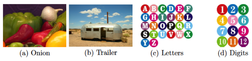
Figure 1: Experimental color images.

We test four different color images, named Onion, Trailer, Letters and Digits; see Fig. 1. For these color images, all algorithms run $50$ iterations and the obtained numerical results are presented on Tables 2-5, respectively. Figures 2-5 present the reconstructed color images $\mathbf{Z}_{50}$. And the relationship between the number of iterations and $\mathrm{log}_{10}(\mathrm{RES}(r))$ for the QNQMF and RGB three channels NMF are plot in Fig. 6.

Table 2: Numerical results of the color image Onion $($$135\times 198$ pixels$)$.

$l$	Method	QIPGM	QADMM	RIPGM	RADMM
10	Time(s)	0.2013	0.0963	0.0146	0.0064
	PSNR	79.8477	81.4198	79.2830	80.4876
20	Time(s)	0.2456	0.1434	0.0160	0.0076
	PSNR	80.4340	83.4851	79.4373	81.6233
30	Time(s)	0.2953	0.1847	0.0211	0.0100
	PSNR	80.7172	85.0360	79.5825	83.9558
40	Time(s)	0.3398	0.2243	0.0214	0.0135
	PSNR	80.8676	86.4066	79.4339	84.7264

Table 3: Numerical results of the color image Trailer $($$683\times 1024$ pixels$)$.

$l$	Method	QIPGM	QADMM	RIPGM	RADMM
20	Time(s)	9.7480	3.2211	0.8885	0.1091
	PSNR	84.7805	88.5377	85.8208	88.2529
40	Time(s)	10.2728	3.6850	0.9614	0.1445
	PSNR	84.9515	89.8671	86.2576	89.0544
60	Time(s)	11.3930	4.2889	1.0765	0.1748
	PSNR	85.0318	90.7518	86.1012	89.0008
80	Time(s)	12.0315	4.7420	0.8466	0.2031
	PSNR	85.0520	91.4671	84.6746	89.2806

Table 4: Numerical results of the color image Letters $($$680\times 680$ pixels$)$.

$l$	Method	QIPGM	QADMM	RIPGM	RADMM
10	Time(s)	5.8279	2.0546	0.5159	0.0618
	PSNR	81.7718	83.6386	81.8125	83.5888
20	Time(s)	6.4522	2.1344	0.5311	0.0936
	PSNR	82.1142	85.5912	81.8661	85.3397
30	Time(s)	6.4122	2.1437	0.5181	0.0744
	PSNR	82.2917	87.0045	82.1053	86.4040
40	Time(s)	6.5475	2.2501	0.5641	0.0911
	PSNR	82.3586	88.1478	82.0681	87.2978

Table 5: Numerical results of the color image Digits $($$800\times 800$ pixels$)$.

$l$	Method	QIPGM	QADMM	RIPGM	RADMM
10	Time(s)	8.5460	2.5299	0.8968	0.0930
	PSNR	83.2662	85.0228	82.9325	84.9425
20	Time(s)	8.7719	2.5244	0.8720	0.0989
	PSNR	83.6544	86.7386	83.2849	86.3813
30	Time(s)	8.9382	2.7024	0.8939	0.1104
	PSNR	83.8515	87.9248	83.4227	87.2967
40	Time(s)	9.2815	2.8476	0.9283	0.1337
	PSNR	83.8593	88.9088	83.5650	87.9792

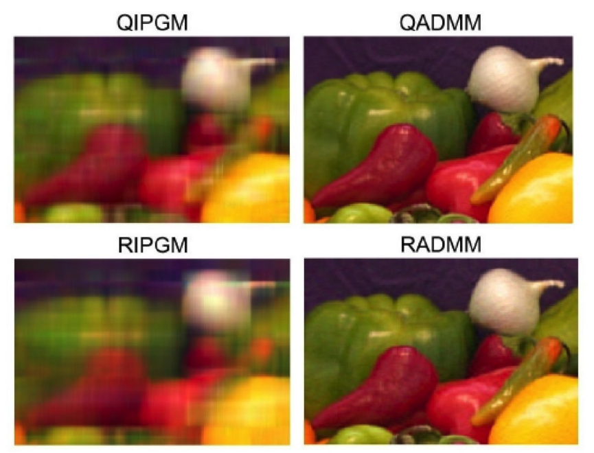
Figure 2: Experimental results of four different algorithms for Onion with $l=40$.

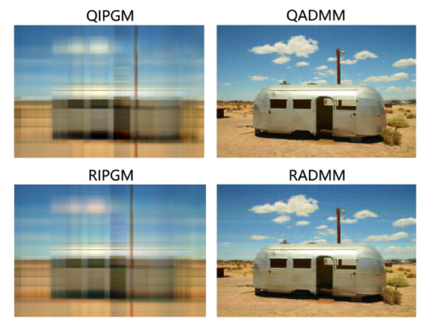
Figure 3: Experimental results of four different algorithms for Trailer with $l=80$.

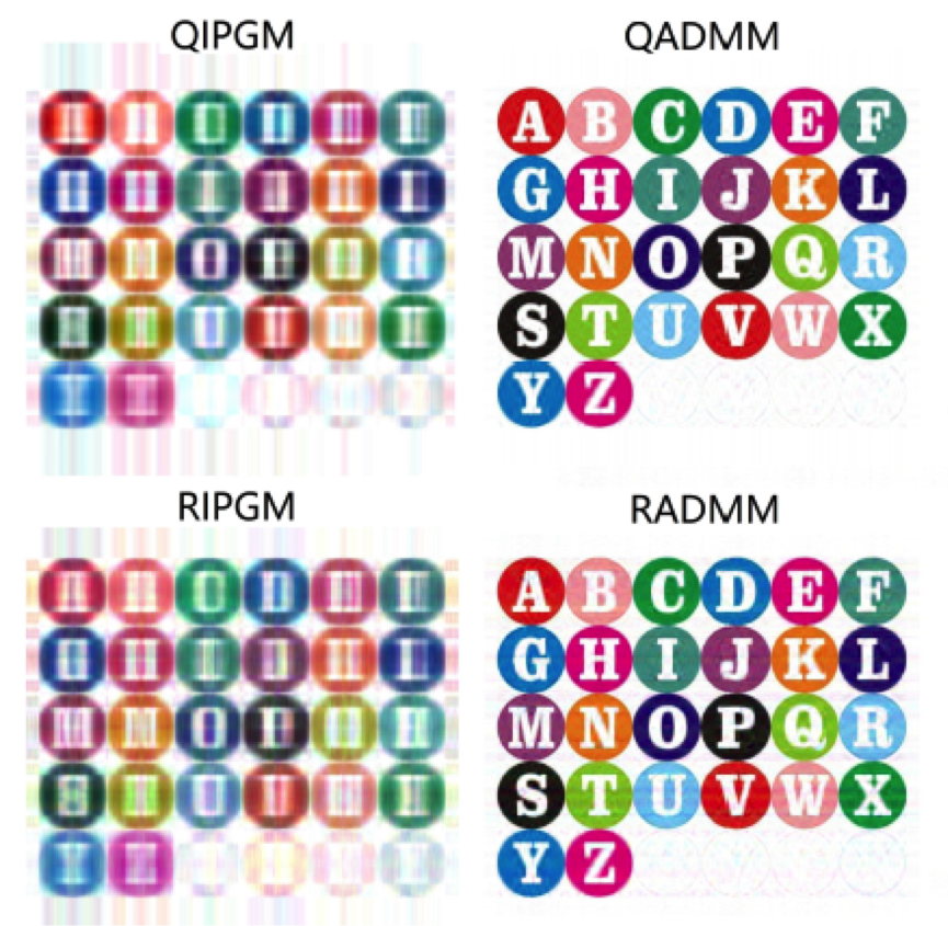
Figure 4: Experimental results of four different algorithms for Letters with $l=40$.

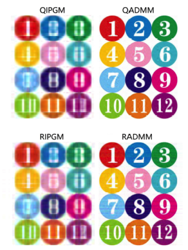
Figure 5: Experimental results of four different algorithms for Digits with $l=40$.

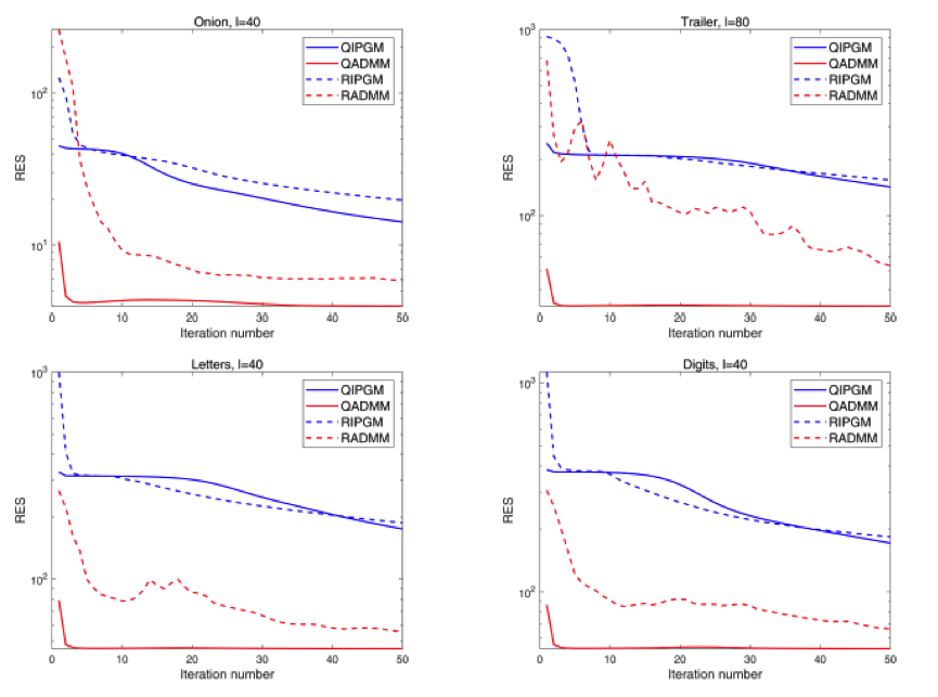
Figure 6: Relationship between the number of iterations and $\mathrm{log}_{10}(\mathrm{RES}(r))$ for different color images.

From these numerical results, the following facts can be observed.

• QIPGM and QADMM cost more CPU time than RIPGM and RADMM at one iteration step. However, the PSNR values of QIPGM and QADMM are better than RIPGM and RADMM, respectively. In other words, these algorithms based on QNQMF take more CPU time at one iteration step, but they have better numerical performances than the corresponding algorithms based on NMF.

• For QIPGM and RIPGM, the sequences $\{\mathrm{RES}(r)\}$ are monotonically nonincreasing from Fig. 6, which is a manifestation of Lemma 3.7. Since QIPGM and RIPGM need to search the step sizes $\alpha_{r}$ and $\beta_{r}$ at each iteration step, it will take a lot of CPU time. Thus, the CPU time of QIPGM is the maximum of these compared algorithms.

• The PSNR value of QADMM is the best from Tables 2-5. In addition, we can see that QADMM just need few number of iterations to reach the minimum residual value $\mathrm{RES}(r)$; see Fig. 6. Moreover, the recovered image via QADMM is the sharpest in the image quality; see Figures 2-5. In particular, for QADMM and RADMM, it is very obvious increase in the PSNR value as the value $l$ increases.

5.2 Color face recognition

Suppose that $\mathbf{Q}=Q_{R}{\bf i}+Q_{G}{\bf j}+Q_{B}{\bf k}\in\mathbb{Q}^{m\times n}$ represents a color face image with $Q_{R}$, $Q_{G}$ and $Q_{B}$ being respectively the red, green, and blue values of pixels. Suppose that the training set contains $\mu$ known face image, denoted by $\mathbb{T}=\{\mathbf{F}_{1},\mathbf{F}_{2},\ldots,\mathbf{F}_{\mu}\}$ and the testing set contains $\nu$ face image to be recognized, denoted by $\mathbb{S}=\{\mathbf{G}_{1},\mathbf{G}_{2},\ldots,\mathbf{G}_{\nu}\}$. Here, $\mathbf{F}_{t}(t=1,2,\ldots,\mu)$ and $\mathbf{G}_{s}(s=1,2,\ldots,\nu)$ are $mn\times 1$ pure quaternion vectors, which are obtained via straighten $m\times n$ color face images into the columns.

Let $\mathbf{X}=(\mathbf{F}_{1},\mathbf{F}_{2},\ldots,\mathbf{F}_{\mu})$ and $l$ be the positive integer. Assume that the basis images are $\mathbf{W}=(\mathbf{w}_{1},\mathbf{w}_{2},\ldots,\mathbf{w}_{l})$ and the encodings are $\mathbf{H}=(\mathbf{h}_{1},\mathbf{h}_{2},\ldots,\mathbf{h}_{\mu})$. Since the QNQMF

$$\mathbf{X}=\mathbf{W}\mathbf{H},$$

the each face $\mathbf{F}_{t}$ can be approximately reconstructed by

$$\mathbf{F}_{t}=\mathbf{W}\mathbf{h}_{t},\quad t=1,2,\ldots,\mu.$$

In Algorithm 5.2, we present the color face recognition based on the QNQMF.

 

 

Step 0. Input the color face images in

$$\mathbb{T}=\{\mathbf{F}_{1},\mathbf{F}_{2},\ldots,\mathbf{F}_{\mu}\}\quad and\quad\mathbb{S}=\{\mathbf{G}_{1},\mathbf{G}_{2},\ldots,\mathbf{G}_{\nu}\}.$$

Let the training data $\mathbf{X}_{train}=(\mathbf{F}_{1},\mathbf{F}_{2},\ldots,\mathbf{F}_{\mu})$.

Step 1. Do QNQMF:

$$\mathbf{X}_{train}=\mathbf{W}_{train}\mathbf{H}_{train}.$$

Step 2. For $s=1,2,\ldots,\nu$, compute

$$\mathbf{h}_{s}=(\mathbf{W}_{train}^{*}\mathbf{W}_{train})^{-1}(\mathbf{W}_{train}^{*}\mathbf{G}_{s})$$

and

$$\theta_{t,s}=\frac{\mathrm{Re}\,\langle\mathbf{h}_{s},~{}\mathbf{H}_{train}(:,t)\rangle}{\|\mathbf{h}_{s}\|_{F}\|\mathbf{H}_{train}(:,t)\|_{F}},\quad t=1,\ldots,\mu.$$ (36)

Let

$$t_{\circledast}=\mathrm{argmax}_{1\leq t\leq\mu}\,\theta_{t,s}.$$

Such $\mathbf{F}_{t_{\circledast}}$ is the optimum matching encoding for the trained image $\mathbf{G}_{s}$.

 

In (36), $\mathbf{H}_{train}(:,t)$ denotes the $t$-th column of the quasi non-negative quaternion matrix $\mathbf{H}_{train}$ and the similarity measure $\theta_{t,s}$ determines the matching score between $\mathbf{h}_{s}$ and $\mathbf{H}_{train}(:,t)$, which is corresponding to $\mathbf{G}_{s}$ in the testing set and $\mathbf{F}_{t}$ in the training set. When we test on the gray face images, ${h}_{s}$ and ${H}_{train}(:,t)$ reduce to the real vectors and the value

$$\theta_{t,s}=\frac{\langle{h}_{s},~{}{H}_{train}(:,t)\rangle}{\|{h}_{s}\|_{2}\|{H}_{train}(:,t)\|_{2}}$$ (37)

is the cosine angle between the two vectors. Hence, the maximum similarity measure means the best matching trained image. We remark that the authors in [33] divided the color image into the red, green, blue color channels and proposed the following Algorithm 4.

 

Algorithm 4  Color face recognition based on color channels NMF [33]

 

Step 0. Input the color face images in

$$\mathbb{T}=\{\mathbf{F}_{1},\mathbf{F}_{2},\ldots,\mathbf{F}_{\mu}\}\quad and\quad\mathbb{S}=\{\mathbf{G}_{1},\mathbf{G}_{2},\ldots,\mathbf{G}_{\nu}\},$$

where $\mathbf{F}_{t}=F_{R,t}\mathbf{i}+F_{G,t}\mathbf{j}+F_{B,t}\mathbf{k}$ for $t=1,2,\ldots,\mu$ and $\mathbf{G}_{s}=G_{R,s}\mathbf{i}+G_{G,s}\mathbf{j}+G_{B,s}\mathbf{k}$ for $s=1,2,\ldots,\nu$. Let the training matrices

$$\left\{\begin{array}[]{l}X_{R,train}=(F_{R,1},F_{R,2},\ldots,F_{R,\mu}),\\ X_{G,train}=(F_{G,1},F_{G,2},\ldots,F_{G,\mu}),\\ X_{B,train}=(F_{B,1},F_{B,2},\ldots,F_{B,\mu})\end{array}\right.$$

be the red, green, and blue values of pixels, respectively.

Step 1. Do NMF on real field:

$$\left\{\begin{array}[]{l}X_{R,train}=W_{R,train}H_{R,train},\\ X_{G,train}=W_{G,train}H_{G,train},\\ X_{B,train}=W_{B,train}H_{B,train}.\\ \end{array}\right.$$

Step 2. For $s=1,2,\ldots,\nu$, compute

$$\left\{\begin{array}[]{l}h_{R,s}=(W_{R,train}^{*}W_{R,train})^{-1}(W_{R,train}^{*}G_{R,s}),\\ h_{G,s}=(W_{G,train}^{*}W_{G,train})^{-1}(W_{G,train}^{*}G_{G,s}),\\ h_{B,s}=(W_{B,train}^{*}W_{B,train})^{-1}(W_{B,train}^{*}G_{B,s})\end{array}\right.$$

and

$$\theta_{t,s}=\frac{\langle h_{R,s},\,H_{R,train}(:,t)\rangle}{\|h_{R,s}\|_{2}\|H_{R,train}(:,t)\|_{2}}+\frac{\langle h_{G,s},\,H_{G,train}(:,t)\rangle}{\|h_{G,s}\|_{2}\|H_{G,train}(:,t)\|_{2}}+\frac{\langle h_{B,s},\,H_{B,train}(:,t)\rangle}{\|h_{B,s}\|_{2}\|H_{B,train}(:,t)\|_{2}}$$

for $t=1,\ldots,\mu$. Let

$$t_{\circledast}=\mathrm{argmax}_{1\leq t\leq\mu}\,\theta_{t,s}.$$

Such $\mathbf{F}_{t_{\circledast}}$ is the optimum matching encoding for the trained image $\mathbf{G}_{s}$.

In this subsection, we utilize QNQMF to the color face recognition. From the results presented in Subsection 5.1, we know that the numerical performance of ADMM-like method is good. Thus, we study the ADMM-like method for the face recognition.

Here, we compare the following these algorithms.

• QADMM-color: Algorithm 5.2 with Algorithm 3 for the color face images;

• RADMM-color: Algorithm 4 with the iteration (34) for the color face images;

• RADMM-gray: the iteration (34) with (37) for the gray face images;

• QPCA-color: the quaternion principal component analysis for the color face images [21].

In addition, the paraments $\alpha=0.01$ and $\beta=0.01$ for QADMM-color, RADMM-color and RADMM-gray methods. For QPCA-color, the value $l$ means the first $l$ largest eigenvalues and corresponding eigenvectors. The accuracy rate is defined as

$$\mathrm{Rate}=\dfrac{\text{True~{}Numbers}}{\text{Total Numbers}}.$$

Example 5.1.

In this experiment, we focus on the famous CASIA 3D face database [36]. CASIA 3D face database involves $123$ individuals and each individual contains $37$ or $38$ different color face images with $640\times 480$ pixels. We focus on the first $37$ images for each individual. The training set is randomly selected with the random number $\eta(=20,24,28,32)$ and the remaining as the testing set. All the color face images are cropped as the $100\times 100$ pixels, then resized to $50\times 50$ pixels. Fig. 7 presents the faces from the first one $($just the first $36$ images$)$. The pictures show not only the single variations of poses, expressions and illuminations, but also the combined variations of expressions under illumination and poses under expressions. We preserve a small amount of face information for some images after processing.

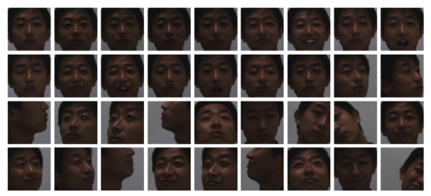
Figure 7: Cropped color face images from CASIA 3D face database.

Table 6: Numerical results of Example 5.1 $(\eta=20)$.

Method	$l$	$3$	$6$	$9$	$12$	$15$
QADMM-color	Time(s)	33.2277	33.6415	34.0056	34.5794	36.7154
	Rate	26.88$\%$	51.79$\%$	67.10$\%$	70.73$\%$	73.17$\%$
RADMM-color	Time(s)	5.5573	5.6143	5.7008	5.7749	5.9524
	Rate	18.08$\%$	51.89$\%$	60.78$\%$	68.48$\%$	71.54$\%$
RADMM-gray	Time(s)	2.8677	2.8651	2.9298	2.9524	3.0534
	Rate	6.70$\%$	38.35$\%$	58.97$\%$	63.27$\%$	67.53$\%$
QPCA-color	Time(s)	54.1980	60.3608	75.4179	87.1528	90.9380
	Rate	37.64$\%$	58.54$\%$	62.94$\%$	66.04$\%$	67.29$\%$

Table 7: Numerical results of Example 5.1 $(\eta=24)$.

Method	$l$	$3$	$6$	$9$	$12$	$15$
QADMM-color	Time(s)	56.4495	59.3814	45.3469	32.6791	58.4169
	Rate	24.77$\%$	45.65$\%$	63.85$\%$	68.04$\%$	72.23$\%$
RADMM-color	Time(s)	8.9977	9.3838	5.2911	5.3229	8.9831
	Rate	16.76$\%$	45.22$\%$	58.79$\%$	68.04$\%$	70.04$\%$
RADMM-gray	Time(s)	3.4718	3.6892	2.6669	2.6659	3.6898
	Rate	6.32$\%$	34.83$\%$	54.91$\%$	64.23$\%$	67.85$\%$
QPCA-color	Time(s)	72.2730	100.6967	117.7804	84.2996	99.1015
	Rate	38.34$\%$	57.22$\%$	62.85$\%$	64.60$\%$	67.92$\%$

Table 8: Numerical results of Example 5.1 $(\eta=28)$.

Method	$l$	$3$	$6$	$9$	$12$	$15$
QADMM-color	Time(s)	52.0266	28.9591	32.5345	47.9965	30.4193
	Rate	22.85$\%$	49.59$\%$	63.69$\%$	68.74$\%$	72.09$\%$
RADMM-color	Time(s)	6.2049	3.9847	6.6568	7.5933	4.2583
	Rate	14.36$\%$	49.59$\%$	60.34$\%$	67.21$\%$	71.73$\%$
RADMM-gray	Time(s)	3.0223	2.0628	3.3289	2.9618	2.0643
	Rate	4.70$\%$	37.85$\%$	56.10$\%$	66.31	68.93$\%$
QPCA-color	Time(s)	96.3664	69.5055	84.6165	134.0832	100.5329
	Rate	36.04$\%$	55.47$\%$	61.52$\%$	63.60$\%$	66.21$\%$

Table 9: Numerical results of Example 5.1 $(\eta=32)$.

Method	$l$	$3$	$6$	$9$	$12$	$15$
QADMM-color	Time(s)	22.4030	22.6615	22.8519	22.9498	23.6767
	Rate	24.88$\%$	50.57$\%$	69.76$\%$	72.68$\%$	76.42$\%$
RADMM-color	Time(s)	2.7697	2.7544	2.7980	2.7596	2.9234
	Rate	15.45$\%$	44.55$\%$	67.80$\%$	72.36$\%$	74.63$\%$
RADMM-gray	Time(s)	1.3816	1.3950	1.4634	1.4897	1.4620
	Rate	5.69$\%$	32.68$\%$	56.91$\%$	68.29$\%$	71.87$\%$
QPCA-color	Time(s)	67.2749	72.5781	95.2822	147.7504	104.1266
	Rate	39.67$\%$	60.49$\%$	66.83$\%$	69.11$\%$	70.41$\%$

For Example 5.1, QADMM-color, RADMM-color, RADMM-gray algorithms run 4 iterations and the accuracy rates as well as the CPU time are presented on Tables 6-9 for different dimensions $l$ and the random numbers $\eta$.

Example 5.2.

In this experiment, we focus on the famous AR face database [29]. We select randomly $100$ individuals $($$50$ males and $50$ females$)$. Each individual contains $26$ different color face images with $165\times 120$ pixels, including frontal views of with different facial expressions, lighting conditions and occlusions. The training set is randomly selected with the random number $\lambda(=14,16,18,20)$ and the remaining as the testing set. All the color face images are resized to $80\times 60$ pixels. Fig. 8 presents the faces from one of the male individuals.

For Example 5.2, the QADMM-color, RADMM-color and RADMM-gray algorithms run 4 iterations and the accuracy rates as well as the CPU time are presented on Tables 10-13 for different dimensions $l$ and the values $\lambda$.

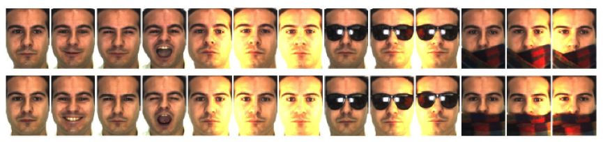
Figure 8: Original color face images from AR face database.

Table 10: Numerical results of Example 5.2 $(\lambda=14)$.

Method	$l$	$5$	$10$	$15$	$20$	$25$
QADMM-color	Time(s)	8.3088	8.4811	8.7379	8.9954	9.0350
	Rate	30.58$\%$	42.67$\%$	57.00$\%$	64.58$\%$	68.08$\%$
RADMM-color	Time(s)	2.3156	2.3267	2.3678	2.4297	2.4932
	Rate	27.58$\%$	41.83$\%$	53.83$\%$	61.25$\%$	66.92$\%$
RADMM-gray	Time(s)	1.0397	1.0343	1.0205	1.0834	1.0727
	Rate	18.92$\%$	33.75$\%$	45.92$\%$	54.92$\%$	59.67$\%$
QPCA-color	Time(s)	13.4900	18.8405	21.8072	27.3111	32.1785
	Rate	33.33$\%$	43.42$\%$	46.75$\%$	50.58$\%$	53.50$\%$

Table 11: Numerical results of Example 5.2 $(\lambda=16)$.

Method	$l$	$5$	$10$	$15$	$20$	$25$
QADMM-color	Time(s)	8.9551	8.9055	9.1517	9.3072	9.6715
	Rate	39.20$\%$	58.50$\%$	65.60$\%$	70.40$\%$	74.40$\%$
RADMM-color	Time(s)	1.9035	1.9908	1.9718	2.0098	2.1245
	Rate	34.30$\%$	57.10$\%$	60.60$\%$	68.20$\%$	72.70$\%$
RADMM-gray	Time(s)	0.9110	0.9376	0.9309	0.9337	0.9478
	Rate	24.70$\%$	47.40$\%$	56.00$\%$	62.50$\%$	68.60$\%$
QPCA-color	Time(s)	13.1535	19.2302	21.6543	26.7626	31.7443
	Rate	45.70$\%$	58.80$\%$	63.90$\%$	67.40$\%$	68.40$\%$

Table 12: Numerical results of Example 5.2 $(\lambda=18)$.

Method	$l$	$5$	$10$	$15$	$20$	$25$
QADMM-color	Time(s)	8.0949	8.5623	8.9744	8.7200	9.6274
	Rate	25.87$\%$	43.13$\%$	50.50$\%$	58.25$\%$	65.50$\%$
RADMM-color	Time(s)	1.8528	1.8479	1.9877	1.9465	2.1142
	Rate	21.75$\%$	42.63$\%$	49.75$\%$	56.25$\%$	62.50$\%$
RADMM-gray	Time(s)	0.8996	0.9225	1.2338	0.8630	0.9577
	Rate	14.62$\%$	34.25$\%$	44.12$\%$	51.00$\%$	59.25$\%$
QPCA-color	Time(s)	13.4892	18.9881	22.0845	27.9783	32.1396
	Rate	33.62$\%$	46.37$\%$	49.13$\%$	51.50$\%$	52.88$\%$

Table 13: Numerical results of Example 5.2 $(\lambda=20)$.

Method	$l$	$5$	$10$	$15$	$20$	$25$
QADMM-color	Time(s)	9.0368	9.1079	9.8130	9.9078	10.2441
	Rate	31.00$\%$	51.50$\%$	65.67$\%$	81.50$\%$	84.17$\%$
RADMM-color	Time(s)	1.5250	1.5520	1.5598	1.6164	1.7145
	Rate	30.83$\%$	50.17$\%$	62.83$\%$	78.00$\%$	82.50$\%$
RADMM-gray	Time(s)	0.7205	0.7291	0.7306	0.8068	0.8167
	Rate	17.67$\%$	40.50$\%$	52.33$\%$	59.83$\%$	69.17$\%$
QPCA-color	Time(s)	13.9676	18.7256	21.7172	27.5337	33.5137
	Rate	34.83$\%$	44.67$\%$	50.83$\%$	54.67$\%$	55.67$\%$

From the results of Examples 5.1 and 5.2, it indicates the following facts.

• The results of Examples 5.1 and 5.2 exhibit the recognition performance and robustness of QADMM-color algorithm, which has the better accuracy rate and less CPU time than QPCA-color algorithm for the larger value $l$. This indicates that QADMM-color algorithm has a good numerical performance.

• QPCA-color algorithm costs the most CPU time even though we use the fast Lanczos method. This is due to that we need to compute the first $l$ largest eigenvalues and corresponding eigenvectors of the covariance matrix from the training set, which is a $2500\times 2500$ quaternion matrix for Example 5.1 or a $4800\times 4800$ quaternion matrix for Example 5.2 .

• When the value $l$ is small, the accuracy rates of QADMM-color and QPCA-color are much higher than RADMM-color and RADMM-gray. This indicates that the algorithms based on the quaternion are better than encoded three color channels of color images and single channel of gray level images. In other word, color images represented the pure quaternion matrices can explore the information between color channels. In addition, with the increase of the dimension $l$, the accuracy rate of face recognition also increases.

6 Concluding remarks

We introduced the QNQMF model and proposed two solving numerical algorithms. Moreover, we explored the advantages of QNQMF for color image reconstruction and color face recognition. From these numerical results, it can see that QNQMF has simple form, good interpretability and small storage space. And the algorithms encoded on the quaternion perform better than the algorithms encoded on the red, green and blue channels. In particular, the QNQMF model has a better face recognition ability and robustness than real NMF model encoded separately on color channels of color images and on single channel of gray level images for the same data.

Acknowledgments The authors are grateful for the Editor-in-Chief, Associate Editor, and Reviewers for their valuable comments and insightful suggestions that helped to improve this research significantly.

Author Contributions The authors have contributed equally in this scholarly work.

Funding This research is supported by the National Natural Science Foundation of China grants 62105064, 41725017, 12171210, 12090011 and 11901098; the Major Projects of Universities in Jiangsu Province of China grants 21KJA110001; and the Natural Science Foundation of Fujian Province of China grants 2020J05034.

Appendix A The real representation method

In this appendix, we analysis the real representation method.

Remark that (3) is equivalent to

$$\Upsilon_{\mathbf{X}}=\Upsilon_{\mathbf{W}}\Upsilon_{\mathbf{H}},$$ (38)

or

$$\left\{\begin{array}[]{c}X_{0}=W_{0}H_{0}-W_{1}H_{1}-W_{2}H_{2}-W_{3}H_{3},\\ X_{1}=W_{0}H_{1}+W_{1}H_{0}+W_{2}H_{3}-W_{3}H_{2},\\ X_{2}=W_{0}H_{2}-W_{1}H_{3}+W_{2}H_{0}+W_{3}H_{1},\\ X_{3}=W_{0}H_{3}+W_{1}H_{2}-W_{2}H_{1}+W_{3}H_{0}\\ \end{array}\right.$$ (39)

with $W_{1},W_{2},W_{3}\geq 0$ and $H_{1},H_{2},H_{3}\geq 0$.

For the equivalent problem (38), it is quite expansive to solve as the dimension-expanding problem caused by the real counterpart method. Meanwhile, it is different from NMF (2); thus those numerical algorithms proposed for NMF will not directly applied to solve (38). And for the problem (39), it will be difficult to comprehend adequately the structure of quaternion quasi non-negative matrices $\mathbf{W}$ and $\mathbf{H}$ if $W_{0},W_{1},W_{2},W_{3}$ and $H_{0},H_{1},H_{2},H_{3}$ are as separate variables.

In fact, the optimization problem (5) is equivalent to

$$\begin{array}[]{ll}\min&f(\mathbf{W},\mathbf{H})=\|X_{0}-(W_{0}H_{0}-W_{1}H_{1}-W_{2}H_{2}-W_{3}H_{3})\|_{F}^{2}\\ &\qquad\qquad~{}~{}+\|X_{1}-(W_{0}H_{1}+W_{1}H_{0}+W_{2}H_{3}-W_{3}H_{2})\|_{F}^{2}\\ &\qquad\qquad~{}~{}+\|X_{2}-(W_{0}H_{2}-W_{1}H_{3}+W_{2}H_{0}+W_{3}H_{1})\|_{F}^{2}\\ &\qquad\qquad~{}~{}+\|X_{3}-(W_{0}H_{3}+W_{1}H_{2}-W_{2}H_{1}+W_{3}H_{0})\|_{F}^{2},\\ \mathrm{s.t.}&W_{1}\geq 0,~{}W_{2}\geq 0,~{}W_{3}\geq 0,~{}H_{1}\geq 0,~{}H_{2}\geq 0,~{}H_{3}\geq 0.\end{array}$$ (40)

Now, we consider the Karush-Kuhn-Tucker (KKT) optimality conditions of the optimization problem (40). Let $y=(y_{1}^{T},y_{2}^{T},\ldots,y_{8}^{T})^{T}\in\mathbb{R}^{4l(m+n)}$ with

$$\begin{array}[]{llll}y_{1}=\mathrm{vec}(W_{0}),&y_{2}=\mathrm{vec}(W_{1}),&y_{3}=\mathrm{vec}(W_{2}),&y_{4}=\mathrm{vec}(W_{3}),\\ y_{5}=\mathrm{vec}(H_{0}),&y_{6}=\mathrm{vec}(H_{1}),&y_{7}=\mathrm{vec}(H_{2}),&y_{8}=\mathrm{vec}(H_{3}),\\ \end{array}$$

and

$$\begin{array}[]{lll}G_{1,s,t}(y)=(W_{1})_{st},&G_{2,s,t}(y)=(W_{2})_{st},&G_{3,s,t}(y)=(W_{3})_{st},\\ J_{1,t,k}(y)=(H_{1})_{tk},&J_{2,t,k}(y)=(H_{2})_{tk},&J_{3,t,k}(y)=(H_{3})_{tk}\\ \end{array}$$

for $s=1,\ldots,m$, $t=1,\ldots,l$ and $k=1,\ldots,n$.

Suppose that $\widehat{y}$ is a local minimum of the problem (40). Denote

$$\mathbb{I}_{G}(\widehat{y})=\{(a,s,t)\,|\,G_{a,s,t}(\widehat{y})=0\},~{}~{}\mathbb{I}_{J}(\widehat{y})=\{(b,t,k)\,|\,J_{b,t,k}(\widehat{y})=0\}.$$

It is obvious that $f$, $G_{a,s,t}(a=1,2,3;s=1,\ldots,m;t=1,\ldots,l)$ and $J_{b,t,k}(b=1,2,3;t=1,\ldots,l;k=1,\ldots,n)$ are continuously differentiable functions over $\mathbb{R}^{4l(m+n)}$. And it is easy to verify that the gradients of the active constraints

$$\{\nabla G_{a,s,t}(\widehat{y})\}_{(a,s,t)\in\mathbb{I}_{G}(\widehat{y})}\cup\{\nabla J_{b,t,k}(\widehat{y})\}_{(b,t,k)\in\mathbb{I}_{J}(\widehat{y})}$$

are linearly independent. Then, there exist multipliers $c_{a,s,t}(a=1,2,3;s=1,\ldots,m;t=1,\ldots,l)$ and $d_{b,t,k}(b=1,2,3;t=1,\ldots,l;k=1,\ldots,n)$ such that

$$\left\{\begin{array}[]{l}\nabla f(\widehat{y})-\sum_{a,s,t}c_{a,s,t}\nabla G_{a,s,t}(\widehat{y})-\sum_{b,t,k}d_{b,t,k}\nabla J_{b,t,k}(\widehat{y})=0,\\ G_{a,s,t}(\widehat{y})\geq 0,~{}~{}~{}~{}c_{a,s,t}\geq 0,~{}~{}~{}~{}c_{a,s,t}G_{a,s,t}(\widehat{y})=0,\\ J_{b,t,k}(\widehat{y})\geq 0,~{}~{}~{}~{}~{}d_{b,t,k}\geq 0,~{}~{}~{}~{}d_{b,t,k}J_{b,t,k}(\widehat{y})=0,\end{array}\right.$$ (41)

where $a,b=1,2,3;$ $s=1,\ldots,m;$ $t=1,\ldots,l$ and $k=1,\ldots,n$. Let the matrices $C_{a}=(c_{a,s,t})\in\mathbb{R}^{m\times l}$ with $a=1,2,3$ and $D_{b}=(d_{b,t,k})\in\mathbb{R}^{l\times n}$ with $b=1,2,3$. Then, if $(\widehat{\mathbf{W}},\widehat{\mathbf{H}})$ corresponding with $\widehat{y}$ is a local minimum of the problem (40), from (41), we have

$$\left\{\begin{array}[]{l}\nabla_{W_{0}}f(\widehat{\mathbf{W}},\widehat{\mathbf{H}})=0,~{}~{}\nabla_{H_{0}}f(\widehat{\mathbf{W}},\widehat{\mathbf{H}})=0,\\ \nabla_{W_{1}}f(\widehat{\mathbf{W}},\widehat{\mathbf{H}})-C_{1}=0,~{}~{}W_{1}\geq 0,~{}~{}C_{1}\geq 0,~{}~{}W_{1}\odot C_{1}=0,\\ \nabla_{W_{2}}f(\widehat{\mathbf{W}},\widehat{\mathbf{H}})-C_{2}=0,~{}~{}W_{2}\geq 0,~{}~{}C_{2}\geq 0,~{}~{}W_{2}\odot C_{2}=0,\\ \nabla_{W_{3}}f(\widehat{\mathbf{W}},\widehat{\mathbf{H}})-C_{3}=0,~{}~{}W_{3}\geq 0,~{}~{}C_{3}\geq 0,~{}~{}W_{3}\odot C_{3}=0,\\ \nabla_{H_{1}}f(\widehat{\mathbf{W}},\widehat{\mathbf{H}})-D_{1}=0,~{}~{}H_{1}\geq 0,~{}~{}D_{1}\geq 0,~{}~{}H_{1}\odot D_{1}=0,\\ \nabla_{H_{2}}f(\widehat{\mathbf{W}},\widehat{\mathbf{H}})-D_{2}=0,~{}~{}H_{2}\geq 0,~{}~{}D_{2}\geq 0,~{}~{}H_{2}\odot D_{2}=0,\\ \nabla_{H_{3}}f(\widehat{\mathbf{W}},\widehat{\mathbf{H}})-D_{3}=0,~{}~{}H_{3}\geq 0,~{}~{}D_{3}\geq 0,~{}~{}H_{3}\odot D_{3}=0.\end{array}\right.$$ (42)

According to (42), we can obtain the KKT optimality conditions of the problem (5), that is (8).

Appendix B Proofs of Lemmas 3.1, 3.2 and 3.3

In this appendix, we present the proofs of lemmas in Section 3.

Define the matrix set

$$\mathbb{R}_{\dagger}^{m\times 4n}:=\{R=(R_{0},R_{1},R_{2},R_{3})\in\mathbb{R}^{m\times 4n}\,|\,R_{0}\in\mathbb{R}^{m\times n},R_{1},R_{2},R_{3}\in\mathbb{R}_{+}^{m\times n}\},$$

where $\mathbb{R}_{+}^{m\times n}$ is the non-negative set on the real field. Hence, the sets $\mathbb{Q}_{\dagger}^{m\times n}$ and $\mathbb{R}_{\dagger}^{m\times 4n}$ are isomorphic.

It is obvious that $\mathbb{R}_{\dagger}^{m\times 4n}$ is a nonempty closed convex set, and let $\mathcal{P}_{\mathbb{R}_{\dagger}^{m\times 4n}}$ be the projection into $\mathbb{R}_{\dagger}^{m\times 4n}$, which is defined by

$$\mathcal{P}_{\mathbb{R}_{\dagger}^{m\times 4n}}(R):=\mathrm{argmin}\,\|Y-R\|_{F},\quad\forall\,Y\in\mathbb{R}_{\dagger}^{m\times 4n},$$

then we can obtain that

$$\mathcal{P}_{\mathbb{R}_{\dagger}^{m\times n}}(R)=(R_{0},~{}\mathcal{P}_{+}(R_{1}),~{}\mathcal{P}_{+}(R_{2}),~{}\mathcal{P}_{+}(R_{3})),$$

where $\mathcal{P}_{+}(R_{s})=\max(R_{s},0)$, $s=1,2,3$.

Proof of Lemma 3.1. Let $\mathbf{X}=X_{0}+X_{1}{\bf i}+X_{2}{\bf j}+X_{3}{\bf k}$, $\mathbf{W}=W_{0}+W_{1}{\bf i}+W_{2}{\bf j}+W_{3}{\bf k}$ and $\mathbf{H}=H_{0}+H_{1}{\bf i}+H_{2}{\bf j}+H_{3}{\bf k}$. Since

$$\mathbf{W}\mathbf{H}= (W_{0}H_{0}-W_{1}H_{1}-W_{2}H_{2}-W_{3}H_{3})+(W_{0}H_{1}+W_{1}H_{0}+W_{2}H_{3}-W_{3}H_{2}){\bf i}$$

$$+(W_{0}H_{2}-W_{1}H_{3}+W_{2}H_{0}+W_{3}H_{1}){\bf j}+(W_{0}H_{3}+W_{1}H_{2}-W_{2}H_{1}+W_{3}H_{0}){\bf k}$$

$$:= M_{0}+M_{1}{\bf i}+M_{2}{\bf j}+M_{3}{\bf k}$$

and

$$\frac{1}{2}\|\mathbf{X}-\mathbf{W}\mathbf{H}\|_{F}^{2}=\frac{1}{2}(\|X_{0}-M_{0}\|_{F}^{2}+\|X_{1}-M_{1}\|_{F}^{2}+\|X_{2}-M_{2}\|_{F}^{2}+\|X_{3}-M_{3}\|_{F}^{2}),$$

according to (6), we can get that

$$\nabla_{\mathbf{W}}f(\mathbf{W},\mathbf{H})=\frac{\partial f(\mathbf{W},\mathbf{H})}{\partial W_{0}}+\frac{\partial f(\mathbf{W},\mathbf{H})}{\partial W_{1}}{\bf i}+\frac{\partial f(\mathbf{W},\mathbf{H})}{\partial W_{2}}{\bf j}+\frac{\partial f(\mathbf{W},\mathbf{H})}{\partial W_{3}}{\bf k}$$

$$= (X_{0}-M_{0})(-H_{0}^{T})+(X_{1}-M_{1})(-H_{1}^{T})+(X_{2}-M_{2})(-H_{2}^{T})+(X_{3}-M_{3})(-H_{3}^{T})$$

$$+[(X_{0}-M_{0})(H_{1}^{T})+(X_{1}-M_{1})(-H_{0}^{T})+(X_{2}-M_{2})(H_{3}^{T})+(X_{3}-M_{3})(-H_{2}^{T})]{\bf i}$$

$$+[(X_{0}-M_{0})(H_{2}^{T})+(X_{1}-M_{1})(-H_{3}^{T})+(X_{2}-M_{2})(-H_{0}^{T})+(X_{3}-M_{3})(H_{1}^{T})]{\bf j}$$

$$+[(X_{0}-M_{0})(H_{3}^{T})+(X_{1}-M_{1})(H_{2}^{T})+(X_{2}-M_{2})(-H_{1}^{T})+(X_{3}-M_{3})(-H_{0}^{T})]{\bf k}$$

$$= -(\mathbf{X}-\mathbf{W}\mathbf{H})\mathbf{H}^{*}.$$

Similarly, we can get that $\nabla_{\mathbf{H}}f(\mathbf{W},\mathbf{H})=-\mathbf{W}^{*}(\mathbf{X}-\mathbf{W}\mathbf{H})$.

Proof of Lemma 3.2. It is obvious that if the point $(\widehat{\mathbf{W}},\widehat{\mathbf{H}})$ satisfies (8), then it meets (9). We will show next that conversely: if (9) holds, then the point $(\widehat{\mathbf{W}},\widehat{\mathbf{H}})$ also meets (8).

Case 1: if $\mathrm{Re}\,\nabla_{\mathbf{W}}f(\widehat{\mathbf{W}},\widehat{\mathbf{H}})\neq 0$, then there exist $s_{0}$ and $t_{0}$ such that $a_{0}:=(\mathrm{Re}\,\nabla_{\mathbf{W}}f(\widehat{\mathbf{W}},\widehat{\mathbf{H}}))_{s_{0},t_{0}}\neq 0$. Let

$$\mathbf{Y}_{st}=\left\{\begin{array}[]{ll}\widehat{\mathbf{W}}_{st}-a_{0},&{if}~{}s=s_{0},~{}t=t_{0},\\ \widehat{\mathbf{W}}_{st},&{others}.\\ \end{array}\right.$$

As $\widehat{\mathbf{W}}\in\mathbb{Q}_{\dagger}^{m\times l}$, thus we have $\mathbf{Y}\in\mathbb{Q}_{\dagger}^{m\times l}$ and

$$\mathrm{Re}\,[\langle\nabla_{\mathbf{W}}f(\widehat{\mathbf{W}},\widehat{\mathbf{H}}),~{}\mathbf{Y}-\widehat{\mathbf{W}}\rangle]=-a_{0}^{2}<0,$$

which is contradict with the first inequality of (9).

Case 2: if $\nabla_{\mathbf{W}}f(\widehat{\mathbf{W}},\widehat{\mathbf{H}})\not\in\mathbb{Q}_{\dagger}^{m\times l}$, there exist $s_{0}$ and $t_{0}$ such that one of the following three inequalities

$$\left\{\begin{array}[]{l}(\mathrm{Im}_{i}\,\nabla_{\mathbf{W}}f(\widehat{\mathbf{W}},\widehat{\mathbf{H}}))_{s_{0},t_{0}}<0,\\ (\mathrm{Im}_{j}\,\nabla_{\mathbf{W}}f(\widehat{\mathbf{W}},\widehat{\mathbf{H}}))_{s_{0},t_{0}}<0,\\ (\mathrm{Im}_{k}\,\nabla_{\mathbf{W}}f(\widehat{\mathbf{W}},\widehat{\mathbf{H}}))_{s_{0},t_{0}}<0\\ \end{array}\right.$$

holds. Without loss of generality, assume that $a_{1}:=(\mathrm{Im}_{i}\,\nabla_{\mathbf{W}}f(\widehat{\mathbf{W}},\widehat{\mathbf{H}}))_{s_{0},t_{0}}<0$. Let

$$\mathbf{Y}_{st}=\left\{\begin{array}[]{ll}\widehat{\mathbf{W}}_{st}-a_{1}\mathbf{i},&{if}~{}s=s_{0},~{}t=t_{0},\\ \widehat{\mathbf{W}}_{st},&{others}.\\ \end{array}\right.$$

Then, $(\mathrm{Im}_{i}\,\mathbf{Y})_{s_{0},t_{0}}=(\mathrm{Im}_{i}\,\widehat{\mathbf{W}})_{s_{0},t_{0}}-a_{1}>0$. Thus, we have $\mathbf{Y}\in\mathbb{Q}_{\dagger}^{m\times l}$ and

$$\mathrm{Re}\,[\langle\nabla_{\mathbf{W}}f(\widehat{\mathbf{W}},\widehat{\mathbf{H}}),~{}\mathbf{Y}-\widehat{\mathbf{W}}\rangle]=-a_{1}^{2}<0,$$

which is contradict with the first inequality of (9).

Case 3: if $\mathrm{Im}_{i}\,\widehat{\mathbf{W}}\odot\mathrm{Im}_{i}\,\nabla_{\mathbf{W}}f(\widehat{\mathbf{W}},\widehat{\mathbf{H}})\neq 0,$ there exist $s_{0}$ and $t_{0}$ such that

$$\widehat{w}_{1}:=(\mathrm{Im}_{i}\,\widehat{\mathbf{W}})_{s_{0},t_{0}}>0,\quad a_{1}:=(\mathrm{Im}_{i}\,\nabla_{\mathbf{W}}f(\widehat{\mathbf{W}},\widehat{\mathbf{H}}))_{s_{0},t_{0}}>0.$$

Let

$$\mathbf{Y}_{st}=\left\{\begin{array}[]{ll}0,&{if}~{}s=s_{0},~{}t=t_{0},\\ \widehat{\mathbf{W}}_{st},&{others}.\\ \end{array}\right.$$

Then, we have $\mathbf{Y}\in\mathbb{Q}_{\dagger}^{m\times l}$ and

$$\mathrm{Re}\,[\langle\nabla_{\mathbf{W}}f(\widehat{\mathbf{W}},\widehat{\mathbf{H}}),~{}\mathbf{Y}-\widehat{\mathbf{W}}\rangle]=-\widehat{w}_{1}a_{1}<0,$$

which is contradict with the first inequality of (9).

If $\mathrm{Im}_{j}\,\widehat{\mathbf{W}}\odot\mathrm{Im}_{j}\,\nabla_{\mathbf{W}}f(\widehat{\mathbf{W}},\widehat{\mathbf{H}})\neq 0$ and $\mathrm{Im}_{k}\,\widehat{\mathbf{W}}\odot\mathrm{Im}_{k}\,\nabla_{\mathbf{W}}f(\widehat{\mathbf{W}},\widehat{\mathbf{H}})\neq 0$, we can also show that they are contradict with the first inequality of (9). Hence, if the first inequality of (9) holds if and only if $\widehat{\mathbf{W}}$ satisfies (8).

Similarly, it can verify that the second inequality of (9) holds if and only if $\widehat{\mathbf{H}}$ satisfies (8).

Proof of Lemma 3.3. Let $\mathbf{Y}=Y_{0}+Y_{1}{\bf i}+Y_{2}{\bf j}+Y_{3}{\bf k}\in\mathbb{Q}^{m\times n}$ and $\mathbf{Z}=Z_{0}+Z_{1}{\bf i}+Z_{2}{\bf j}+Z_{3}{\bf k}\in\mathbb{Q}^{m\times n}$.

We prove the result (1). If $\mathbf{Z}\in\mathbb{Q}_{\dagger}^{m\times n}$, it follows that

$$\mathrm{Re}\,[\langle\mathcal{P}_{\mathbb{Q}_{\dagger}^{m\times n}}(\mathbf{Y})-\mathbf{Y},~{}\mathbf{Z}-\mathcal{P}_{\mathbb{Q}_{\dagger}^{m\times n}}(\mathbf{Y})\rangle]=\sum_{s=1}^{3}\langle\mathcal{P}_{+}(Y_{s})-Y_{s},~{}Z_{s}-\mathcal{P}_{+}(Y_{s})\rangle\geq 0,$$

which is based on the fact $\langle\mathcal{P}_{+}(a)-a,~{}b-\mathcal{P}_{+}(a)\rangle\geq 0$ for any $a\in\mathbb{R}$ and $b\in\mathbb{R}_{+}$.

We prove the result (2). It follows that

$$\begin{array}[]{ll}&\mathrm{Re}\,[\langle\mathcal{P}_{\mathbb{Q}_{\dagger}^{m\times n}}(\mathbf{Y})-\mathcal{P}_{\mathbb{Q}_{\dagger}^{m\times n}}(\mathbf{Z}),\mathbf{Y}-\mathbf{Z}\rangle]\\ &=\langle Y_{0}-Z_{0},Y_{0}-Z_{0}\rangle+\sum_{s=1}^{3}\langle\mathcal{P}_{+}(Y_{s})-\mathcal{P}_{+}(Z_{s}),~{}Y_{s}-Z_{s}\rangle\geq 0,\end{array}$$

which is based on the fact $\langle\mathcal{P}_{+}(a)-\mathcal{P}_{+}(b),~{}a-b\rangle\geq 0$ for any $a,b\in\mathbb{R}$. It is obvious that $\mathcal{P}_{\mathbb{Q}_{\dagger}^{m\times n}}(\mathbf{Y})\neq\mathcal{P}_{\mathbb{Q}_{\dagger}^{m\times n}}(\mathbf{Z})$, then the strict inequality holds.

We prove the result (3). It follows that

$$\begin{array}[]{ll}&\|\mathcal{P}_{\mathbb{Q}_{\dagger}^{m\times n}}(\mathbf{Y})-\mathcal{P}_{\mathbb{Q}_{\dagger}^{m\times n}}(\mathbf{Z})\|_{F}^{2}=\|Y_{0}-Z_{0}\|_{F}^{2}+\sum_{s=1}^{3}\|\mathcal{P}_{+}(Y_{s})-\mathcal{P}_{+}(Z_{s})\|_{F}^{2}\\ &\leq\|Y_{0}-Z_{0}\|_{F}^{2}+\sum_{s=1}^{3}\|Y_{s}-Z_{s}\|_{F}^{2}=\|\mathbf{Y}-\mathbf{Z}\|_{F}^{2},\end{array}$$

which is based on the fact $|\mathcal{P}_{+}(a)-\mathcal{P}_{+}(b)|\leq|a-b|$ for any $a,b\in\mathbb{R}$.

References

- [1] Ang, A.M.S., Gillis, N.: Accelerating nonnegative matrix factorization algorithms using extrapolation. Neural Comput. 31(2), 417-439 (2019)
- [2] Bertsekas, D.P.: On the Goldstein-Levitin-Polyak gradient projection method. IEEE Trans. Automat. Contr. 21(2), 174-184 (1976)
- [3] Boyd, S., Parikh, N., Chu, E., Peleato, B., Eckstein, J.: Distributed optimization and statistical learning via the alternating direction method of multipliers. Found. Trends Mach. Learn. 3(1), 1-122 (2011)
- [4] Calamai, P.P., Mor, J.J.: Projected gradient methods for linearly constrained problems. Math. Program. 39, 93-116 (1987)
- [5] Chen, Y., Jia, Z.G., Peng, Y., Zhang, D.: A new structure-preserving quaternion QR decomposition method for color image blind watermarking. Signal Process. 185, 108088 (2021)
- [6] Chen, Y.N., Qi, L.Q., Zhang, X.Z., Xu, Y.W.: A low rank quaternion decomposition algorithm and its application in color image inpainting. arXiv:2009.12203 (2020)
- [7] Cichocki, A., Zdunek, R.: Regularized alternating least squares algorithms for non-negative matrix/tensor factorization. Advances in Int. Symposium on Neural Networks, Springer, Berlin, Heidelberg 793-802 (2007)
- [8] Flamant, J., Miron, S., Brie, D.: Quaternion non-negative matrix factorization: Definition, uniqueness, and algorithm. IEEE Trans. Signal Process. 68, 1870-1883 (2020)
- [9] Gafni, E.M., Bertsekas, D.P.: Convergence of a gradient projection method. Report LIDS-P-1201, Lab. for Info. and Dec. Systems, M.I.T. (1982)
- [10] Glowinski, R., Marrocco, A.: Sur l’approximation par elements finis d’ordre un, et la resolution par penalisation-dualite d’une classe de problemes de Dirichlet nonlineaires. ESAIM: Mathematical Moddelling and Numerical Analysis Modlisation Mathmatique et Analyse Numrique 9, 41-76 (1975)
- [11] Gong, P.H., Zhang, C.S.: Efficient nonnegative matrix factorization via projected Newton method. Pattern Recogn. 45(9), 3557-3565 (2012)
- [12] Guan, N.Y., Tao, D.C., Luo, Z.G., Yuan, B.: NeNMF: an optimal gradient method for nonnegative matrix factorization. IEEE Trans. Signal Process. 60, 2882-2898 (2012)
- [13] Hajinezhad, D., Chang, T.H., Wang, X.F., Shi, Q.J., Hong, M.Y.: Nonnegative matrix factorization using ADMM: Algorithm and convergence analysis. In International Conference on Acoustics, Speech and Signal Processing (ICASSP), IEEE, 4742-4746 (2016)
- [14] Hamilton, W.R.: Elements of Quaternions. Longmans Green, London (1866)
- [15] Huang, C.Y., Fang, Y.Y., Wu, T.T., Zeng, T.Y., Zeng, Y.H.: Quaternion screened Poisson equation for low-light image enhancement. IEEE Signal Process. Lett. 29, 1417-1421 (2022)
- [16] Huang, C.Y., Li, Z., Liu, Y.B., Wu, T.T., Zeng, T.Y.: Quaternion-based weighted nuclear norm minimization for color image restoration. Pattern Recogn. 128, 108665 (2022)
- [17] Jia, Z.G.: The Eigenvalue Problem of Quaternion Matrix: Structure-Preserving Algorithms and Applications. Science Press, Beijing (2019)
- [18] Jia, Z.G., Ng, M.K.: Structure preserving quaternion generalized minimal residual method. SIAM J. Matrix Anal. Appl. 42(2), 616-634 (2021)
- [19] Jia, Z.G., Jin, Q.Y., Ng, M.K., Zhao, X.L.: Non-local robust quaternion matrix completion for large-scale color image and video inpainting. IEEE Trans. Image Process. 31, 3868-3883 (2022)
- [20] Jia, Z.G., Ng, M.K., Song, G.J.: Robust quaternion matrix completion with applications to image inpainting. Numer. Linear Algebra Appl. 26(4), e2245 (2019)
- [21] Jia, Z.G., Ng, M.K., Song, G.J.: Lanczos method for large-scale quaternion singular value decomposition. Numer. Algor. 82, 699-717 (2019)
- [22] Jia, Z.G., Ng, M.K., Wang, W.: Color image restoration by saturation-value total variation. SIAM J. Imaging Sci. 12(2), 972-1000 (2019)
- [23] Kim, H., Park, H.: Nonnegative matrix factorization based on alternating nonnegativity constrained least squares and active set method. SIAM J. Matrix Anal. Appl. 30(2), 713-730 (2008)
- [24] Lee, D.D., Seung, H.S.: Learning the parts of objects by non-negative matrix factorization. Nature 401, 788-791 (1999)
- [25] Li, J.Z., Yu, C.Y., Gupta, B.B., Ren, X.C.: Color image watermarking scheme based on quaternion Hadamard transform and Schur decomposition. Multimed. Tools Appl. 77(4), 4545-4561 (2018)
- [26] Lin, C.J.: Projected gradient methods for nonnegative matrix factorization. Neural Comput. 19(10), 2756-2779 (2007)
- [27] Liu, Q.H., Ling, S.T., Jia, Z.G.: Randomized quaternion singular value decomposition for low-rank matrix approximation. SIAM J. Sci. Comput. 44(2), A870-A900 (2022)
- [28] Lu, X.Q., Wu, H., Yuan, Y.: Double constrained NMF for hyperspectral unmixing. IEEE Trans. Geosci. Remote. Sens. 52(5), 2746-2758 (2013)
- [29] Martinez, A.M., Benavente, R.: The AR Face Database. CVC Technical Report 24 (1998)
- [30] Paatero, P., Tapper, U.: Positive matrix factorization: A non-negative factor model with optimal utilization of error estimates of data values. Environmetrics 5, 111-126 (1994)
- [31] Pompili, F., Gillis, N., Absil, P.A., Glineur, F.: Two algorithms for orthogonal nonnegative matrix factorization with application to clustering. Neurocomputing 141, 15-25 (2014)
- [32] Qi, L.Q., Luo, Z.Y., Wang Q.W., Zhang, X.Z.: Quaternion matrix optimization: Motivation and analysis. J. Optim. Theory Appl. 193(1), 621-648 (2022)
- [33] Rajapakse, M., Tan, J., Rajapakse, J.C.: Color channel encoding with NMF for face recognition. 2004 International Conference on Image Processing, IEEE (2004)
- [34] Rapin, J., Bobin, J., Larue, A., Starck, J.L.: NMF with sparse regularizations in transformed domains. SIAM J. Imaging Sci. 7(4), 2020-2047 (2014)
- [35] Song, G.J., Ding, W.Y., Ng, M.K.: Low rank pure quaternion approximation for pure quaternion matrices. SIAM J. Matrix Anal. Appl. 42(1), 58-82 (2021)
- [36] The CASIA 3D Face Database. http://www.cbsr.ia.ac.cn/english/3dface%20databases.asp
- [37] Wu, T.T., Mao, Z.H., Li, Z.Y., Zeng, Y.H., Zeng, T.Y.: Efficient color image segmentation via quaternion-based / Regularization. J. Sci. Comput. 93(1), 1-26 (2022)
- [38] Xiao, X.L., Zhou, Y.C.: Two-dimensional quaternion PCA and sparse PCA. IEEE Trans. Neur. Net. Lear. 30(7), 2028-2042 (2018)
- [39] Xu, Y.Y., Yin, W.T.: A block coordinate descent method for regularized multiconvex optimization with applications to nonnegative tensor factorization and completion. SIAM J. Imaging Sci. 6(3), 1758-1789 (2013)
- [40] Zhang, S.F., Huang, D.Y., Xei, L., Chng, E.S., Li, H.Z., Dong, M.H.: Non-negative matrix factorization using stable alternating direction method of multipliers for source separation. In Asia-Pacific Signal and Information Processing Association Annual Summit and Conference (APSIPA), IEEE, 222-228 (2015)
- [41] Zhao, M.X., Jia, Z.G., Cai, Y.F., Chen, X., Gong, D.W.: Advanced variations of two-dimensional principal component analysis for face recognition. Neurocomputing 452, 653-664 (2021)