The Force Balance of Electrons During Kinetic Anti-parallel Magnetic Reconnection

Abstract

Fully kinetic simulations are applied to the study of 2D anti-parallel reconnection, elucidating the dynamics by which the electron fluid maintains force balance within both the ion diffusion region (IDR) and the electron diffusion region (EDR). Inside the IDR, magnetic field-aligned electron pressure anisotropy (${p_{e\parallel}}\gg{p_{e\perp}})$ develops upstream of the EDR. Compared to previous investigations, the use of modern computer facilities allows for simulations at the natural proton to electron mass ratio $m_{i}/m_{e}=1836$. In this high-$m_{i}/m_{e}$-limit the electron dynamics changes qualitatively, as the electron inflow to the EDR is enhanced and mainly driven by the anisotropic pressure. Using a coordinate system with the $x$-direction aligned with the reconnecting magnetic field and the $y$-direction aligned with the central current layer, it is well-known that for the much studied 2D laminar anti-parallel and symmetric scenario the reconnection electric field at the $X$-line must be balanced by the $\partial p_{exy}/\partial x$ and $\partial p_{eyz}/\partial z$ off-diagonal electron pressure stress components. We find that the electron anisotropy upstream of the EDR imposes large values of $\partial p_{exy}/\partial x$ within the EDR, and along the direction of the reconnection $X$-line this stress cancels with the stress of a previously determined theoretical form for $\partial p_{eyz}/\partial z$. The electron frozen-in law is instead broken by pressure tensor gradients related to the direct heating of the electrons by the reconnection electric field. The reconnection rate is free to adjust to the value imposed externally by the plasma dynamics at larger scales.

I Introduction

Magnetic reconnection Dungey (1953) is the process that permits the magnetic topology of an electrically conducting plasma to rearrange, often accompanied by large scale release of stored magnetic energy. Well-known instances of reconnection occur in association with solar flares Masuda et al. (1994) and magnetic storms in the Earth’s magnetosphere McPherron, Russell, and Aubry (1973). In resistive MHD models, reconnection is a slow diffusive process within narrow current layers Parker (1957). In low collisional plasma, however, additional physical effects become important as the theoretical width of the resistive current layers fall below the ion skin-depth $d_{i}=c/\omega_{pi}$. Here $c$ is the speed of light and $\omega_{pi}$ is the ion plasma frequency. In these narrow current layers the ions’ inertia may cause them to decouple from the motion of the magnetic field which has been shown to have dramatic implications for the reconnection process.

To more accurately describe the narrow current layers of reconnection, two-fluid models treat the ions and the electrons as separate fluids and successfully predict both fast reconnection and the basic structure of the reconnection region observed in more advanced kinetic models Birn et al. (2001). The two-fluid reconnection geometry includes an ion diffusion region (IDR) with the width of about $1d_{i}$, and within this region the ion frozen-in condition is broken. Mathematically, this occurs when ${\bf E}+{\bf u}_{i}\times{\bf B}\neq 0$, where ${\bf E}$ and ${\bf B}$ denote the electric and magnetic fields, and ${\bf u}_{i}$ is the ion bulk flow velocity. Meanwhile, the electrons with bulk flow ${\bf u}_{e}$) remain frozen to the field line motion obeying the electron frozen-in law (${\bf E}+{\bf u}_{e}\times{\bf B}=0$) almost all the way into the topological X-line. Ultimately, the frozen-in law is also broken for the electrons within the much smaller electron diffusion region (EDR) with a width of the order of the electron skin-depth, $d_{e}=c/\omega_{pe}$, where $\omega_{pe}$ is the electron plasma frequency. Numerical fluid models which fully resolve $d_{e}$ often break the electron frozen-in law by adding an ad hoc amount of hyper-resistivity (scaling in strength with the Laplacian of the plasma current density, $\nabla^{2}J$) Ohia et al. (2012). An important result of this type of investigations was the realization that the rate of reconnection becomes insensitive to the physics that are responsible for decoupling the electrons from the motion of the magnetic field lines within the EDR Shay et al. (1999).

Despite substantial efforts including laboratory, spacecraft, numerical and theoretical investigations Zweibel and Yamada (2016), a complete understanding of the electron dynamics within the EDR is still not fully developed, and its study is complicated by the process being sensitive to a range of parameters describing a given configuration. Open questions are also concerned with the extent to which 3D effects fundamentally alter the structure of the reconnection region Silin, Büchner, and Vaivads (2005); Che, Drake, and Swisdak (2011); Muñoz, Büchner, and Kilian (2017). However, observations from the Magnetospheric Multiscale (MMS) mission demonstrate that the widths of reconnection layers typically approach the small length scales associated with the local electron orbit width. The length scales perpendicular to a particular reconnection current layer are usually much shorter than the length scale along the current layer, and a range of observations further suggest that the local reconnection dynamics are well captured by 2D laminar models Egedal et al. (2018, 2019); Greess et al. (2021); Schroeder et al. (2022).

The present paper is focused on the case of 2D symmetric and anti-parallel reconnection, which observations suggest is applicable to reconnection in the Earth’s magnetotail. Here, the opposing inflow regions often have similar strength magnetic fields but are oppositely directed Torbert et al. (2018). Our numerical investigation also applies the typical ion to electron temperature ratio, $T_{i}/T_{e}=5$, of the magnetosphere (see Ref. Ma et al. (2020), Fig.4); the results are relatively insensitive to this ratio. Meanwhile, just a small guide-magnetic field in the direction of the current layer can significantly alter the reconnection process, and the present results (obtained with $B_{g}=0$) only apply to cases where $B_{g}\leq 0.05B_{\mbox{\scriptsize rec}}$, corresponding to Regime I reconnection as introduced in Ref. Le et al. (2013). While not explicitly imposed, the number densities of the electrons and ions are always similar, consistent with the condition of quasi-neutrality being well satisfied in the simulations. Thus, throughout the paper we will use $n_{e}=n_{i}\equiv n$.

Within the confines of the closed field lines of the plasma sheet in the Earth’s magnetotail, the normalized electron pressure, $\beta_{e}=nT_{e}/(B/(2\mu_{0}))\simeq 0.1$ is typical Ma et al. (2020). However, if reconnection persists for a sufficient duration, low-$\beta_{e}$ plasma from the lobe regions outside the plasma sheet can reach the reconnection inflows. This can cause a dramatic drop in the plasma inflow density, reducing the electron pressure such that $\beta_{e}\ll 0.1$. For such low values of $\beta_{e}$, the reconnection dynamics change dramatically with the generation of strong electrostatic turbulence including colliding electron holes and double layers Egedal, Daughton, and Le (2012); Egedal et al. (2015). In the present paper, the numerical simulations cover the range $0.008\leq\beta_{e}\leq 0.5$, and the present work is thus limited to the conditions typically observed during symmetric reconnection in the plasma sheet.

For laminar and near steady state reconnection the force balance of the electron fluid is described by the generalized Ohm’s law, which similar to the Navier-Stokes equation for a regular fluid includes pressure and inertial effects:

$${\bf E}+{\bf u}_{e}\times{\bf B}+\frac{\displaystyle 1}{\displaystyle ne}\nabla\cdot{\bf p}_{e}+\frac{\displaystyle m_{e}}{\displaystyle e}{\bf u}_{e}\cdot\nabla{\bf u}_{e}=0\quad.$$ (1)

Here the electron pressure tensor is computed by an integral over the electron phase-space density distribution, ${\bf p}_{e}=m_{e}\int({\bf v}_{e}-{\bf u}_{e})^{2}f_{e}({\bf v}_{e})d^{3}v_{e}$, with ${\bf v}_{e}$ representing the electron velocity. Using a range of kinetic simulations, in the present paper we will discuss how the various terms of Eq. (1) become important within separate spatial areas of the IDR and EDR. Compared to similar investigations a decade or more ago Hesse et al. (1999); Daughton, Scudder, and Homa (2006); Drake, Shay, and Swisdak (2008), a main difference is that modern computing facilities now permit routine fully kinetic simulations at the full proton to electron mass ratio, $m_{i}/m_{e}=1836$. The present analysis reveals that for simulations where this ratio approaches its natural value, ${\bf E}+{\bf u}_{e}\times{\bf B}\simeq 0$ does not apply to the full IDR. The reconnection electric field, $E_{\mbox{\scriptsize rec}}$, is the electric field along the topological $X$-line at the center of the EDR, which by Faraday’s law defines the rate at which magnetic flux it reconnected. For the inner part of the IDR (but still outside what is traditionally considered the EDR Shay, Drake, and Swisdak (2007); Karimabadi, Daughton, and Scudder (2007)) we find that the $|E_{\mbox{\scriptsize rec}}|\ll|\nabla\cdot{\bf p}_{e}/(ne)|$ such that ${\bf u}_{e}\times{\bf B}\simeq-\nabla\cdot{\bf p}_{e}/(ne)$ becomes the main driver of the Hall magnetic field perturbation. In fact, the familiar assumption of $u_{\mbox{\scriptsize in}}=E_{\mbox{\scriptsize rec}}/B_{\mbox{\scriptsize rec,up}}$ significantly underestimates the inflow speed of the electron fluid into the EDR. Here, $B_{\mbox{\scriptsize rec,up}}$ is the in-plane magnetic field just upstream of the EDR.

The main topic of the paper, however, is the development of a theory to explain the terms of Eq. (1) which break the electron frozen-in condition at the very center of the EDR. The study emphasizes the importance of the electron anisotropy upstream of the EDR in driving the current within the EDR and cancelling an off-diagonal stress term identified in previous work Kuznetsova, Hesse, and Winske (1998); Hesse et al. (1999). Ultimately, the off-diagonal stress of ${\bf p}_{e}$, that is responsible for breaking the frozen-in condition, is generated by $E_{\mbox{\scriptsize rec}}$ itself. Thus, the theory suggests that the electron fluid does not represent an obstacle (or bottleneck) for reconnection, which may then proceed at the rate imposed by dynamics external to the EDR. In turn, once reconnection has started, its rate will be controlled by larger scale dynamics which in many cases is well described by MHD models Cassak, Liu, and Shay (2017); Liu et al. (2017). In certain cases including island coalescence it can also be important to retain effects of ion pressure anisotropy Le et al. (2014); Stanier et al. (2015).

The paper is organized as follows: In Section II we discuss previous results on the formation and role of electron pressure anisotropy within the IDR inflow regions, and how it drives the current of the EDR. Section III explores the structure and energy balance of electron flows within the inner part of the IDR, whereas Section IV examines the length scales characterizing the EDR. A detailed account of the electron momentum balance at the $X$-line region is provided in Section V, and the paper is summarized and concluded in Section VI.

II Summary of previous results on the role of electron pressure anisotropy

Our analysis relies strongly on previous results regarding the overall force balance of the EDR Le et al. (2010a); Egedal, Le, and Daughton (2013); Montag, Egedal, and Daughton (2020). For the convenience of the reader, in this section we provide a short summary of this previous work on how the upstream electron pressure anisotropy impacts the structure of the EDR. Additionally, in Appendices A and B we provide additional mathematical considerations to demonstrate how the upstream electron pressure anisotropy drives the current jets within the EDR.

II.1 Formation of electron pressure anisotropy in reconnection inflows, upstream of the EDR

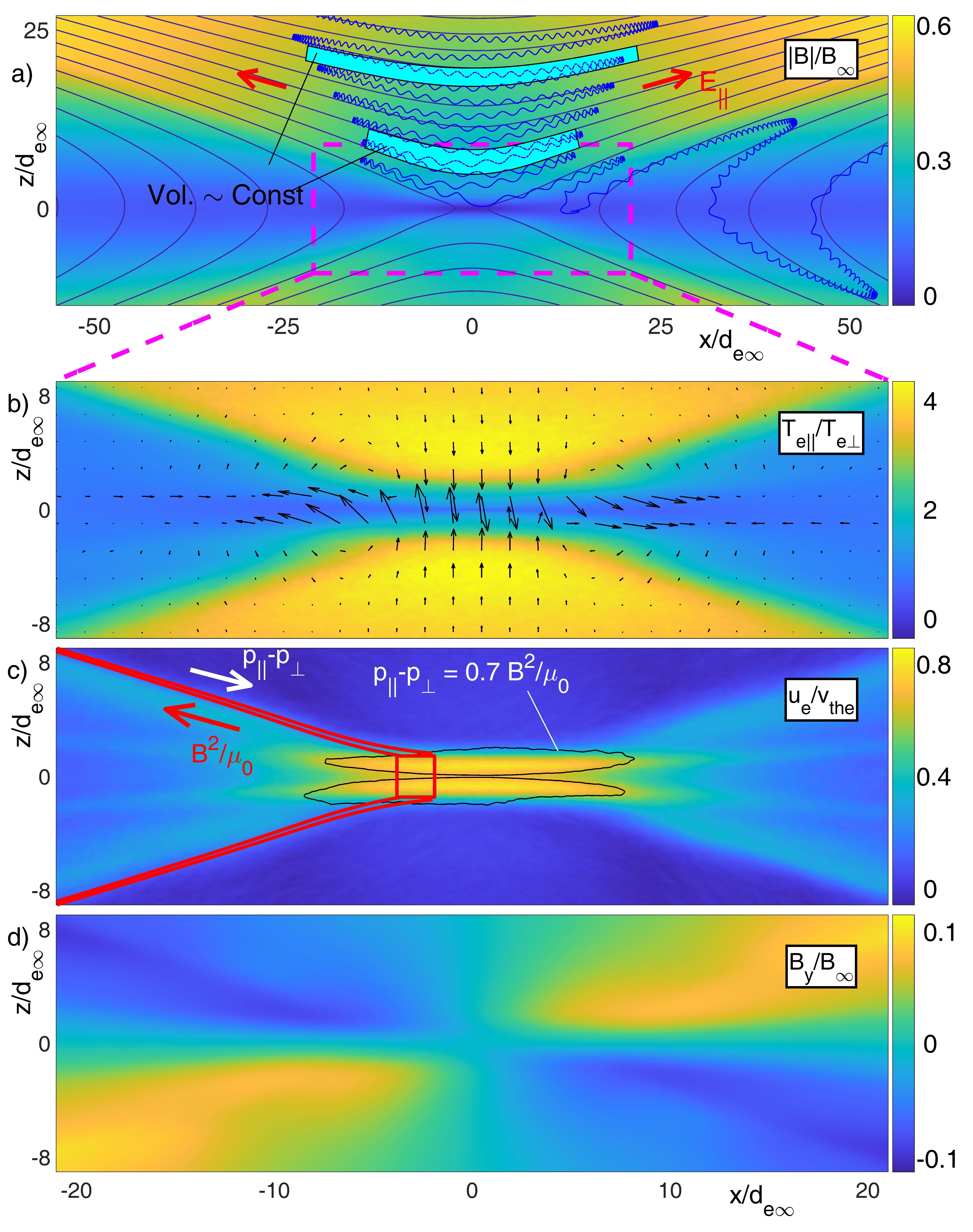
Figure 1: VPIC simulations profiles of a) $B/B_{\infty}$, b) $T_{e\|}/T_{e\perp}$, c) $|{\bf u}_{e}|/v_{te}$, and d) $B_{y}/B_{\infty}$, obtained with $m_{i}/m_{e}=1836$ and $\beta_{e\infty}=2^{-4}=0.0625$. The arrows in b) represent the enhanced electron flow provided by ${\bf J}_{\mbox{\scriptsize extra}}=[({p_{e\parallel}}-{p_{e\perp}})/B]{\bf b}\times\mathbf{\kappa}$.

Due to the trapped orbit dynamics illustrated in Fig. 1(a), it is generally found that the reconnection inflows are characterized by a regime of double adiabatic electron dynamics. It can be shown Le et al. (2009, 2010a) that at the upstream edge of the EDR the main electron pressure components are well described by the CGL-limit Chew, Goldberger, and Low (1956) with ${p_{e\parallel}}\propto n^{3}/B^{2}$ and ${p_{e\perp}}\propto nB$, where $\|$ and $\perp$ denote the directions parallel and perpendicular relative to the local direction of ${\bf B}$. For $\beta_{e\infty}^{2}m_{i}/m_{e}\lesssim 1$ electron holes and double layers yield even stronger ${p_{e\parallel}}$ heating Egedal, Le, and Daughton (2013); Egedal et al. (2015). The effects of the anisotropic heating are evident in the profile in Fig. 1(b), where $T_{e\|}/T_{e\perp}\simeq 4$ is observed just upstream of the EDR, and the marginal electron firehose condition is approached, ${p_{e\parallel}}-{p_{e\perp}}\simeq B^{2}/\mu_{0}$. Within the EDR the adiabatic invariance of the electron magnetic moments, $\mu=m{v_{\perp}}^{2}/(2B)$, break, leading to isotropization and pitch angle mixing. As a result, the electron pressure is approximately isotropic in the reconnection exhaust Le et al. (2013); Egedal et al. (2016).

As described in Appendix A, the physical mechanisms which underpin the CGL-scalings can be understood through relatively simple arguments applicable to the electrons just upstream of the EDR, where the described trapping and parallel compression dynamics (see compressed trapped orbit in Fig. 1(a)) are strong enough to dominate the properties of the electron fluid. A more accurate and rigorous model is provided in Le et al. (2009); Egedal, Le, and Daughton (2013) taking into account that not all electrons become trapped. For the present paper, however, it is sufficient to assume that within the inflow regions the electron pressures approximately follow the aforementioned CGL-scaling laws. While the present simulations use open boundary conditions, the same trapped electron dynamics occur in simulations with periodic boundary conditions Egedal et al. (2009). In contrast to periodic conditions, however, the open system do not need to accommodate the large island of reconnected flux which gets stuck in the periodic reconnection exhausts. Thus, with open boundary conditions a larger fraction of the system is available for the reconnection dynamics Gurram, Egedal, and Daughton (2021).

II.2 Force balance along the length of the EDR and associated scaling laws for the electron pressure anisotropy

In Refs. Le et al. (2010a, b) it was demonstrated that the two dominant terms of Eq. (1) along the EDR are ${\bf u}_{e}\times{\bf B}$ and $(\nabla\cdot{\bf p}_{e})/ne$. Expressed in terms of the Maxwell stress tensor, ${\bf T}=({\bf B}{\bf B}-B^{2}{\bf I})/(2\mu_{0})$, we have $-en{\bf u}_{e}\times{\bf B}\simeq{\bf J}\times{\bf B}=\nabla\cdot{\bf T}$, and momentum balance then requires that $\nabla\cdot({\bf p}_{e}-{\bf T})\simeq 0$. Considering the area encircled by the red square in Fig. 1(c), it can then be shown by the divergence theorem Le et al. (2010a); Montag, Egedal, and Daughton (2020) that at the upstream edge of the EDR the electron firehose condition must be approximately satisfied,

$${p_{e\parallel}^{\mbox{\scriptsize edge}}}-{p_{e\perp}^{\mbox{\scriptsize edge}}}\simeq B_{H}^{2}/\mu_{0}\quad,$$ (2)

where $B_{H}$ represents the magnetic field strength just upstream of the EDR (the direction of this field rotates along the upstream edge of the EDR into the Hall magnetic field explaining the subscript $H$). For example, for the red square in Fig. 1(c) the magnetic tension acting on the sides of the fluid element (corresponding to the integral over the element of the $-en{\bf u}_{e}\times{\bf B}$ force) is offset by pressure anisotropy. Again, this is discussed in more detail in Appendices A and B.

We can derive important scaling laws for the level of pressure anisotropy for locations just upstream of the EDR. Using that ${p_{e\parallel}^{\mbox{\scriptsize edge}}}\gg{p_{e\perp}^{\mbox{\scriptsize edge}}}$ with the CGL-limits the maximal pressure differential

$${\Delta p_{e\|\perp}^{\mbox{\scriptsize max}}}\equiv\mbox{max}({p_{e\parallel}}-{p_{e\perp}})={p_{e\parallel}^{\mbox{\scriptsize edge}}}-{p_{e\perp}^{\mbox{\scriptsize edge}}}\quad,$$ (3)

adheres to the asymptotic scaling ${\Delta p_{e\|\perp}^{\mbox{\scriptsize max}}}\simeq{p_{e\parallel}^{\mbox{\scriptsize edge}}}\simeq(\pi\tilde{n}^{3}/(6\tilde{B}_{H}^{2}))\beta_{e\infty}B_{\infty}^{2}/(2\mu_{0})$. The factor $\pi/6$ is part of the Lê 2009 Equations of State Le et al. (2009), and the $\infty$ subscripts refer to quantities being evaluated far upstream of the IDR, where the electron pressure is assumed to be isotropic. The firehose condition in Eq. (2), representing the dominant momentum balance condition of the EDR, may then be expressed as

$$\frac{\displaystyle B_{H}}{\displaystyle B_{\infty}}=\frac{\displaystyle\mu_{0}K}{\displaystyle 2B_{\infty}}=\left(\frac{\displaystyle\pi\tilde{n}^{3}\beta_{e\infty}}{\displaystyle 12}\right)^{1/4}\quad.$$ (4)

Here $K$ is the integral of the current density across the layer, representing the current per unit length of the EDR. $\tilde{n}\simeq 1$ is the local electron density normalized by the upstream value $n_{\infty}$ (and similar for $\tilde{B}_{H}$ used above) Le et al. (2010a). Eq. (4) is significant as it demonstrates how $K$ is mainly controlled by the external electron pressure anisotropy, which through the CGL-like scalings is set by the normalized upstream electron pressure, $\beta_{e\infty}$.

The above result is in contrast to predictions of two-fluid models with isotropic pressure where ${\bf u}_{e}\times{\bf B}$ is balanced by resistive terms, ${\bf E}$, and/or $(m_{e}/e){\bf u}_{e}\cdot\nabla{\bf u}_{e}$. As discussed below, the half-width $l_{z}\simeq 2d_{e\infty}$ of the EDR region current layer is set by the meandering orbit width Horiuchi and Sato (1997); Shay and Drake (1998); Roytershteyn et al. (2013). From Ampère’s law it then follows that $B_{H}=\mu_{0}enu_{e}l_{z}\simeq 2\mu_{0}enu_{e}d_{e\infty}$, such that $u_{e}=B_{H}/(2enu_{e}d_{e\infty})\simeq B_{H}/(2\sqrt{\mu_{0}nm_{e}})=v_{Ae}/2$. Thus, $u_{e}$ must approach the corresponding value of $\sim v_{Ae}/2$, simply because of the narrow width of the current layer $l_{z}\simeq 2d_{e\infty}$. This analysis is also applicable to the Harris sheet type current layer and the condition $u_{e}=v_{Ae}/2$ is therefore reflective of the underlying meandering orbit dynamics setting the narrow width of the electron flow region Roytershteyn et al. (2013). The EDR current layer direction rotates as a function of $x$ in the $xy$-plane Mandt, Denton, and Drake (1994); Hesse, Zenitani, and Klimas (2008); Le et al. (2010b), and yields the $B_{y}$ perturbations shown in Fig. 1(d) Hesse, Zenitani, and Klimas (2008); Le et al. (2010a). The above results have also been applied in deriving scaling laws for the absolute electron heating within the reconnection inflow and EDR Le, Egedal, and Daughton (2016).

III Electron flows and energy balance within the inner part of the IDR

III.1 Setup of kinetic simulations

The 2D kinetic simulations applied in our study were implemented for anti-parallel Harris sheet reconnection using the code VPIC Bowers et al. (2009) with open boundary conditions Daughton, Scudder, and Homa (2006). The initial magnetic field and the density are $B_{x}=B_{0}\tanh(z/\lambda)$ and $n=n_{0}\cosh^{2}(z/\lambda)+n_{\infty}$, respectively, where $\lambda=0.5d_{i0}=0.5\sqrt{\varepsilon_{0}m_{i}c^{2}/n_{0}e^{2}}$. Other parameters are initial uniform temperatures with $T_{i\infty}/T_{e\infty}=5$, $\omega_{pe0}/\omega_{ce0}=2$, and $\sim 400$ particles per species per cell. The study incorporates 35 separate simulation runs implementing a matrix of 5 values for $m_{i}/m_{e}$ and 7 values for the normalized upstream electron pressure, $\beta_{e\infty}$. To be more specific, we use mass ratios of $m_{i}/m_{e}\in\{100,200,400,800,1836\}$, and the background density $n_{\infty}$ is varied so the initial upstream electron beta is $\beta_{e\infty}=2\mu_{0}n_{\infty}T_{e\infty}/B_{0}^{2}=2^{-k}$ with $k\in\{1,2,\dots,7\}$. In VPIC “natural” units the systems are implemented using $m_{e}=1$, $d_{e0}=1$, $c=1$, $n_{0}=1$, $B_{0}=1/2$, $T_{e\infty}=(1/48)\,m_{e}c^{2}$, and $n_{\infty}/n_{0}=(1+T_{i\infty}/T_{e\infty})2^{-k}$.

For runs with $m_{i}/m_{e}\leq 200$ the domains were $3960\times 1980$ cells, corresponding to $50d_{ip}\times 25d_{ip}$. Runs at $m_{i}/m_{e}\geq 400$ were carried with $5632\times 2816$ cells, corresponding to system sizes of $1000d_{ep}\times 500d_{ep}$. Here, $d_{ip}$ and $d_{ep}$ are the ion and electron skin-depths, respectively, defined with respect to the central peak Harris sheet density, $n_{p}=n_{0}+n_{\infty}$. Furthermore, the upstream electron skin-depth becomes central to our analysis below and can be expressed as $d_{e\infty}=d_{e0}/\sqrt{n_{\infty}/n_{0}}$. For all of the runs, a fixed electron temperature is applied such that $v_{te}/c=0.144=L_{\mbox{\scriptsize Debye}}/d_{e0}$. Measuring the cell size, $\delta$, relative to the Debye length, we then have $\delta/L_{\mbox{\scriptsize Debye}}\simeq(1000/5632)\cdot 0.144\simeq 1.2$, again, based on the initial temperature. The computational cost of the runs scales approximately as $(m_{i}/m_{e})(L_{x}/d_{ep})^{2}$. More details about the similarities and differences between the individual simulation runs are provided in Section IV, where the lengths and widths of the EDR electron jets are examined. In addition, in Table 1 of Appendix D we provide the simulation domain sizes normalized by various parameters.

III.2 The reconnection rate from the perspective of the electrons

Consistent with external MHD scale constraints for system sizes larger than $10d_{i\infty}$ Liu et al. (2017), in the present simulations the absolute reconnection rate obeys $E_{\mbox{\scriptsize rec}}\simeq\alpha v_{A}B$. Here $\alpha\simeq 0.1$ is the normalized reconnection rate, and the relevant Alfvén speed and $B$ are evaluated $1d_{i}$ upstream of the EDR Shay et al. (2004). In our study, values of $E_{\mbox{\scriptsize rec}}$ are computed through a spatial average of $E_{y}$ over a $2d_{e\infty}\times 0.5d_{e\infty}$ region centered on the topological $X$-line. In Fig. 2(a), the corresponding values of $\alpha$ are shown for the full range of our simulations. It should be noted that for $m_{i}/m_{e}=1836$ and $k=7$ the numerical domain only measures about $5d_{i\infty}\times 2.5d_{i\infty}$ (see Table I.C in Appendix D). This could explain the slightly enhanced normalized reconnection rate of $\alpha\simeq 0.14$, which is expected as the “electron-only” regime is approached at small system sizes Phan et al. (2018); Pyakurel et al. (2019); Olson et al. (2021); Greess et al. (2022). Nevertheless, other runs in the set show similar values of $\alpha$ and, as will become clear below, the dynamics recorded for this most extreme run still conform well with the general trends of the full data set.

In Section IV we document how the size of the EDR normalized by $d_{e\infty}$ remains approximately constant for varying values of $m_{i}/m_{e}$. Meanwhile, the size of the IDR scales with $d_{i\infty}=d_{e\infty}\sqrt{m_{i}/m_{e}}$, and from the perspective of the electrons the size of the ion diffusion region thus increases by a factor of $\sqrt{m_{i}/m_{e}}$. Likewise, relative to the time scale of the electron motion, the increasing inertia of the ions will slow the rate of reconnection. As a dimensionless measure of the reconnection electric field relevant to the electron orbit dynamics we introduce $\hat{E}_{\mbox{\scriptsize rec}}=ed_{e\infty}E_{\mbox{\scriptsize rec}}/T_{e\infty}$. This quantity represents the temperature-normalized energy gain an electron will acquire when traveling $d_{e\infty}$ in the direction of $E_{\mbox{\scriptsize rec}}$. Corresponding to the data shown in Fig. 2(b), it then follows that $\hat{E}_{\mbox{\scriptsize rec}}\propto\sqrt{m_{e}/(m_{i}\beta_{e\infty}^{2})}$, where reduced values of $m_{i}/m_{e}$ and low $\beta_{e\infty}$ impose the largest values of $\hat{E}_{\mbox{\scriptsize rec}}$.

In Fig. 2(c) we show the profiles of $T_{e\|}/T_{e\infty}$ and $T_{e\perp}/T_{e\infty}$ corresponding to values in the various runs recorded just upstream of the electron diffusion region. Consistent with the discussion in Section II, for simulations within the double adiabatic regime ($\beta_{e\infty}^{2}m_{i}/m_{e}\gtrsim 1$) marked by the full lines, we observe that both of these profiles are largely independent of $m_{i}/m_{e}$. The normalized electron pressure anisotropy $(p_{e\|}-p_{e\perp})/(n_{\infty}T_{e\infty})$ is then also independent of $m_{i}/m_{e}$, and given the scaling of $\hat{E}_{\mbox{\scriptsize rec}}\propto\sqrt{m_{e}/m_{i}}$ the forces associated with the pressure anisotropy become most significant when compared to $e\hat{E}_{\mbox{\scriptsize rec}}$ at large values of $m_{i}/m_{e}$. In fact, as illustrated in Fig. 2(d) and to be discussed further below, the thermal forces of the electron pressure anisotropy dominate the force balance of the electrons for $m_{i}/m_{e}=1836$, rendering the electron dynamics of the IDR and EDR significantly different when compared to reduced fluid models invoking isotropic electron pressure.

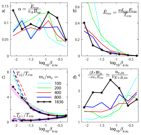
Figure 2: Obtained from a matrix of 35 kinetic simulations, profiles as functions of $\log_{10}(\beta_{e\infty})$ are shown for a range of parameters as marked in the panels. As indicated in c), the line-type denotes the value of $m_{i}/m_{e}$. The “ion-normalized” reconnection rate $\alpha=E_{\mbox{\scriptsize rec}}/(v_{A}B_{up})$ is shown on a) while in b) $\hat{E}_{\mbox{\scriptsize rec}}=ed_{e\infty}E_{\mbox{\scriptsize rec}}/T_{e\infty}$ is the normalized rate relevant to the electron dynamics. In c) the regions shaded in magenta are obtained from the CGL-limit of the Lê-2009 Equations of State Le et al. (2009). The dashed lines mark runs in the regime $\beta_{e\infty}\lesssim\sqrt{m_{i}/m_{e}}$ where additional $T_{e\|}$ heating is typically observed Egedal et al. (2015); Le, Egedal, and Daughton (2016). The profiles in d) show the maximum value of $({\bf J}\times{{\bf B}})_{y}$ observed just upstream of the EDR, normalized by $-en_{\times}E_{\mbox{\scriptsize rec}}$, documenting how forces related to ${\bf J}\times{{\bf B}}$ and $\nabla\cdot{\bf p}_{e}$ dominate at the natural value of $m_{i}/m_{e}$.

III.3 Dominant role of $p_{e\|}\gg p_{e\perp}$ in setting the electron flows and energy dissipation upstream of the EDR

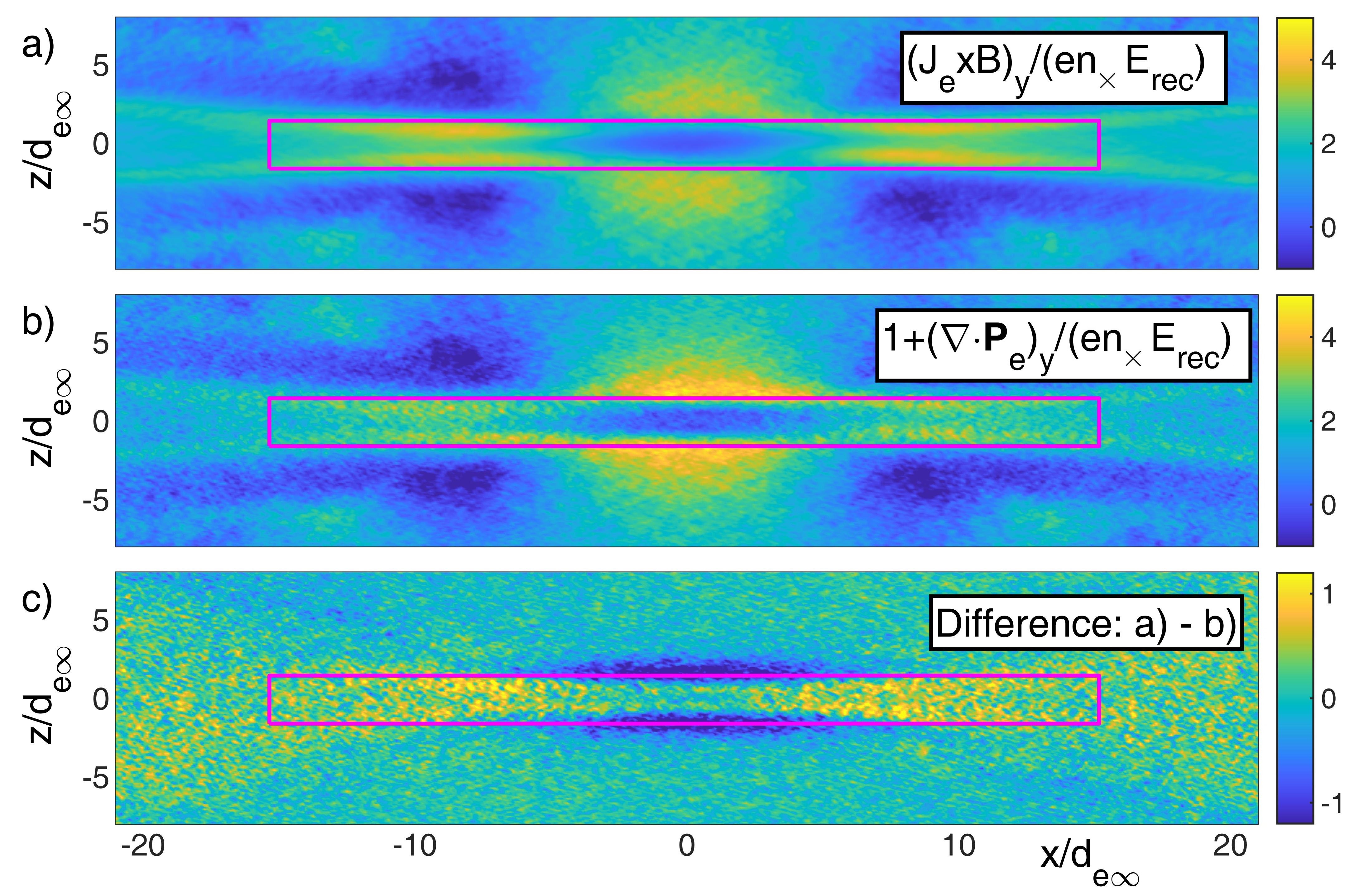
Figure 3: Considering the same simulation as in Fig. 1 ($m_{i}/m_{e}=1836$ and $\beta_{e\infty}=2^{-4}$), color contours are presented for a) the LHS and b) RHS of Eq. (6). The EDR is outlined by the magenta rectangles. For the extended regions where $({\bf J}\times{\bf B})_{y}/(n_{\times}E_{\mbox{\scriptsize rec}})\gtrsim 3.5$ the electron fluid is moving faster than the magnetic field. This motion is driven by electron pressure anisotropy such that $|{\bf J}\times{\bf B}|\simeq|\nabla\cdot{\bf p}_{e}|\gg en_{\times}E_{\mbox{\scriptsize rec}}$. The difference between panels a) and b) is shown in c) and can be attributed to the neglected electron inertia term (note the change in color scale).

In the region outside the EDR where the electrons are well magnetized, the electron pressure anisotropy (${p_{e\parallel}}\gg{p_{e\perp}}$) drives additional currents, ${\bf J}_{\mbox{\scriptsize extra}}=[({p_{e\parallel}}-{p_{e\perp}})/B]{\bf b}\times\mathbf{\kappa}$, via the curvature drift; these currents are not observed for isotropic pressure Egedal, Le, and Daughton (2013). Here $\mathbf{\kappa}=({\bf b}\cdot\nabla){\bf b}$ is the curvature vector, which becomes large where the magnetic field direction, ${\bf b}={\bf B}/B$, has strong spatial variation. In Fig. 1(b) the arrows are proportional to $-{\bf J}_{\mbox{\scriptsize extra}}$ corresponding to a flow boosting the perpendicular drift of electrons into the EDR. ${\bf J}_{\mbox{\scriptsize extra}}$ also has a component in the $y$-direction which drives currents outside the EDR that are in the opposite direction of the electron current within the EDR. While the mathematical expression for ${\bf J}_{\mbox{\scriptsize extra}}$ is not valid inside the EDR, as discussed in Section II the out-of-plane electron current of the EDR can still be attributed to similar effects directly related to ${p_{e\parallel}}\gg{p_{e\perp}}$.

To quantify the relative importance of the flow by ${\bf J}_{\mbox{\scriptsize extra}}$, in Fig. 3 we provide additional profiles for the simulation of Fig. 1, here focusing on the force balance in the $y$-direction in the vicinity of the EDR. Within the IDR we generally have $({\bf u}_{e}\times{\bf B})_{y}\gg({\bf u}_{i}\times{\bf B})_{y}$ and we thus introduce the approximation that $(-en{\bf u}_{e}\times{\bf B})_{y}\simeq({\bf J}\times{\bf B})_{y}$. Consistent with previous work Vasyliunas (1975), generally we have that $\left|({\bf J}\times{\bf B})_{y}\right|\gg\left|(enm_{e}{\bf u}_{e}\cdot\nabla{\bf u}_{e})_{y}\right|$, and the $y$-component of the electron inertia can for the present analysis be neglected. With these approximations the $y$-component of the generalized Ohm’s law in Eq. (1) then becomes Cai, Ding, and Lee (1994)

$$-enE_{y}+({\bf J}\times{\bf B})_{y}=(\nabla\cdot{\bf p}_{e})_{y}\quad.$$ (5)

For the time point considered in Fig. 3 the reconnection geometry and rate is approximately steady. Furthermore, the density profile in this inner region is approximately uniform at a density we denote as $n_{\times}$. It then follows that $nE_{y}\simeq n_{\times}E_{\mbox{\scriptsize rec}}$, where $E_{\mbox{\scriptsize rec}}$ is the value of $E_{y}$ observed at the $X$-line. After dividing Eq. (5) by $en_{\times}E_{\mbox{\scriptsize rec}}$ we obtain:

$$\frac{\displaystyle({\bf J}\times{\bf B})_{y}}{\displaystyle en_{\times}E_{\mbox{\scriptsize rec}}}\simeq 1+\frac{\displaystyle(\nabla\cdot{\bf p}_{e})_{y}}{\displaystyle en_{\times}E_{\mbox{\scriptsize rec}}}\quad.$$ (6)

The LHS (left hand side) of Eq. (6) is shown in Fig. 3(a), while the RHS is shown in Fig. 3(b). The difference between the profiles is relatively small and is shown in Fig. 3(c). This difference can be attributed to the neglected electron inertia in Eq. (6).

From Fig. 3(a) it is apparent that in the vicinity of the EDR $({\bf J}\times{\bf B})_{y}$ is significantly larger than $en_{\times}E_{\mbox{\scriptsize rec}}$. Thus, rather than $enE_{y}\simeq({\bf J}\times{\bf B})_{y}$, we see that $|enE_{y}|\ll|({\bf J}\times{\bf B})_{y}|\simeq|(\nabla\cdot{\bf p}_{e})_{y}|$ in the important inner part of the IDR and throughout most of the EDR. Within the IDR for $x=0$, it is readily shown that $({\bf J}\times{\bf B})_{y}/en_{\times}E_{\mbox{\scriptsize rec}}=u_{e,z}/v_{E\times B,z}$, and the enhanced inflow is provided by $p_{e\|}\gg p_{e\perp}$ through the drifts associated with ${\bf J}_{\mbox{\scriptsize extra}}$. In other words, while $E_{y}$ by Faraday’s law is fundamental for moving the magnetic flux across the reconnection region, Fig. 3 reveals how the $(\nabla\cdot{\bf p}_{e})_{y}$-term is responsible for driving the electrons into the EDR and through the elongated jets of the EDR at high rates, which for the present run are up to 3.5 times the speed of the magnetic field line motion. In Fig. 2(d) the maximum value of $({\bf J}\times{\bf B})_{y}/en_{\times}E_{\mbox{\scriptsize rec}}\,\,(=u_{e,z}/v_{E\times B,z})$ is shown for each of the runs, demonstrating how the enhancement of the inflow speed becomes most pronounced as $m_{i}/m_{e}=1836$ is approached.

The electron pressure anisotropy also has implications for the energy dissipation within the reconnection region. It was recently emphasized Liu et al. (2022) that an electron fluid obeying the frozen-in condition, ${\bf E}=-{\bf v}_{e}\times{\bf B}$, does not exchange any energy with the electromagnetic fields simply because ${\bf J_{e}}\cdot{\bf E}=en{\bf v}_{e}\cdot({\bf v}_{e}\times{\bf B})=0$. This observation is altered by the presence of the strong electron pressure anisotropy. For this case ${\bf E}=-{\bf v}_{e}\times{\bf B}-\nabla\cdot{\bf p}_{e}/(ne)$, such that the now non-zero value of ${\bf J_{e}}\cdot{\bf E}={\bf v}_{e}\cdot(\nabla\cdot{\bf p}_{e})$ permits energy to be exchanged with the fields. In Fig. 4(a) we display the profile of $-{\bf J_{e}}\cdot{\bf E}$, where “yellow” areas with $-{\bf J_{e}}\cdot{\bf E}>0$ are regions where the electrons give energy back to the fields. Such regions, known as generator regions, have been directly observed by the MMS mission Payne et al. (2021).

The continuity of the electromagnetic energy is described by Poynting’s theorem, $-\partial u_{EB}/\partial t=\nabla\cdot{\bf S}+{\bf J}\cdot{\bf E}$, where $u_{EB}=\varepsilon_{0}E^{2}/2+B^{2}/(2\mu_{0})$ is the electromagnetic field energy density and ${\bf S}={\bf E}\times{\bf B}/\mu_{0}$ is the Poynting flux. The profile of $\nabla\cdot{\bf S}$ is shown in Fig. 4(b), which closely resembles the profile of $-{\bf J}_{e}\cdot{\bf E}$. The difference in Fig. 4(c) is the energy either exchanged with $u_{EB}$ and/or the ions through ${\bf J}_{i}\cdot{\bf E}$. The smallness of this difference is consistent with a steady state scenario with steady energy density of the fields throughout the region.

As indicated above, the identified generator regions just upstream of the EDR are a direct consequence of the electron pressure anisotropy that develops in the inflow regions. This is emphasized when comparing $-{\bf J_{e}}\cdot{\bf E}$ in Fig. 4(a) with $-{\bf J}_{\mbox{\scriptsize extra}}\cdot{\bf E}_{z}$ in Fig. 4(d). Again, the expression for ${\bf J}_{\mbox{\scriptsize extra}}$ is not valid within the EDR. Nevertheless, the predicted values of ${\bf J}_{\mbox{\scriptsize extra}}\cdot{\bf E}_{z}$ demonstrate that the main contributor to ${\bf J_{e}}\cdot{\bf E}$ at the edge of the EDR are the curvature-drift-driven currents that enhance the inflow of the electrons into the strong $E_{z}$ electric fields on the EDR’s edge. The structure of $E_{z}$ will be discussed in further details below.

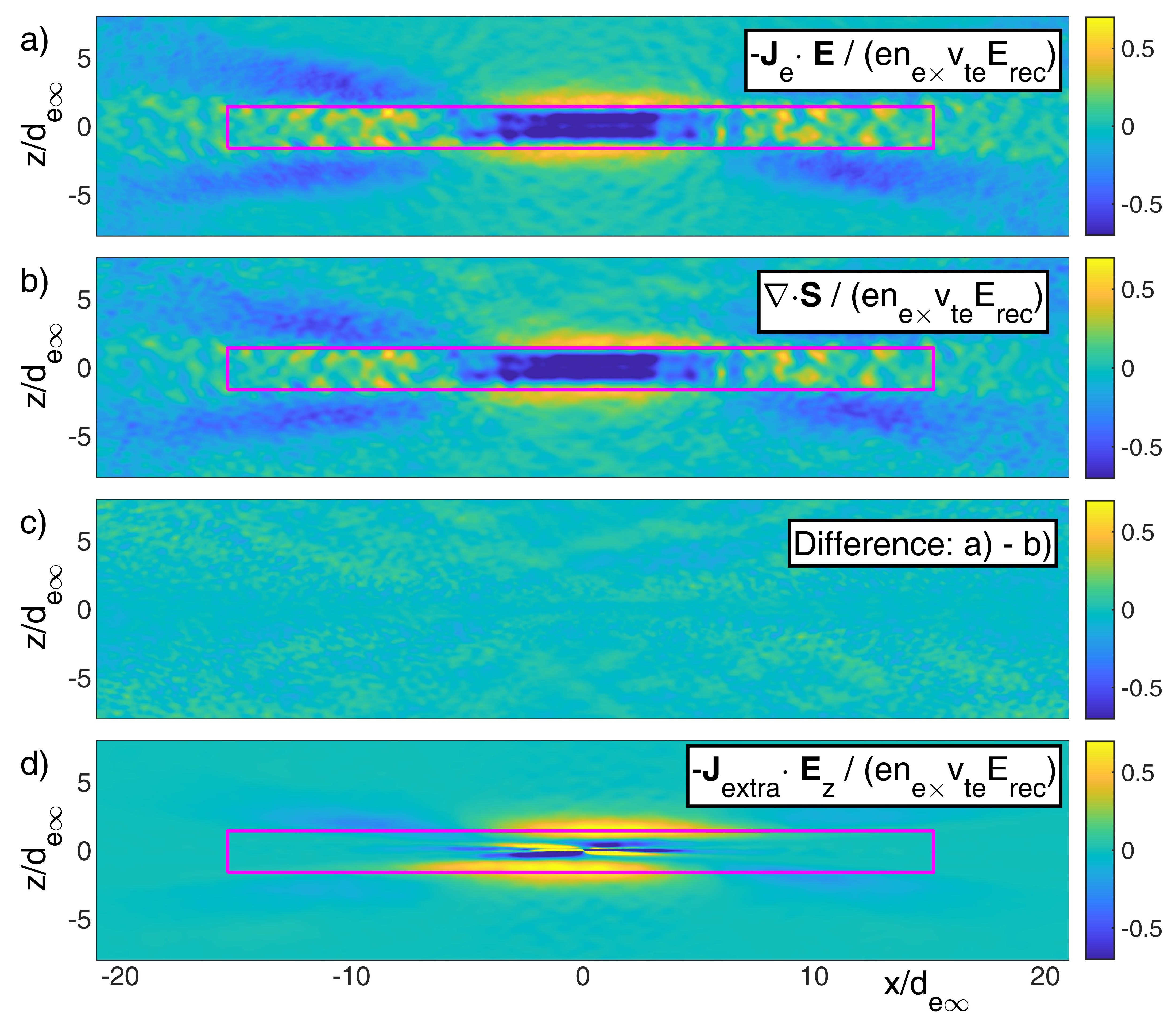
Figure 4: a,b) Near identical profiles of $-{\bf J}_{e}\cdot{\bf E}$ and $\nabla\cdot{\bf S}$, representing the main two terms in Poynting’s theorem. Their difference is shown in c). The profile of $-{\bf J}_{\mbox{\scriptsize extra}}\cdot{\bf E}_{z}$ is shown d).

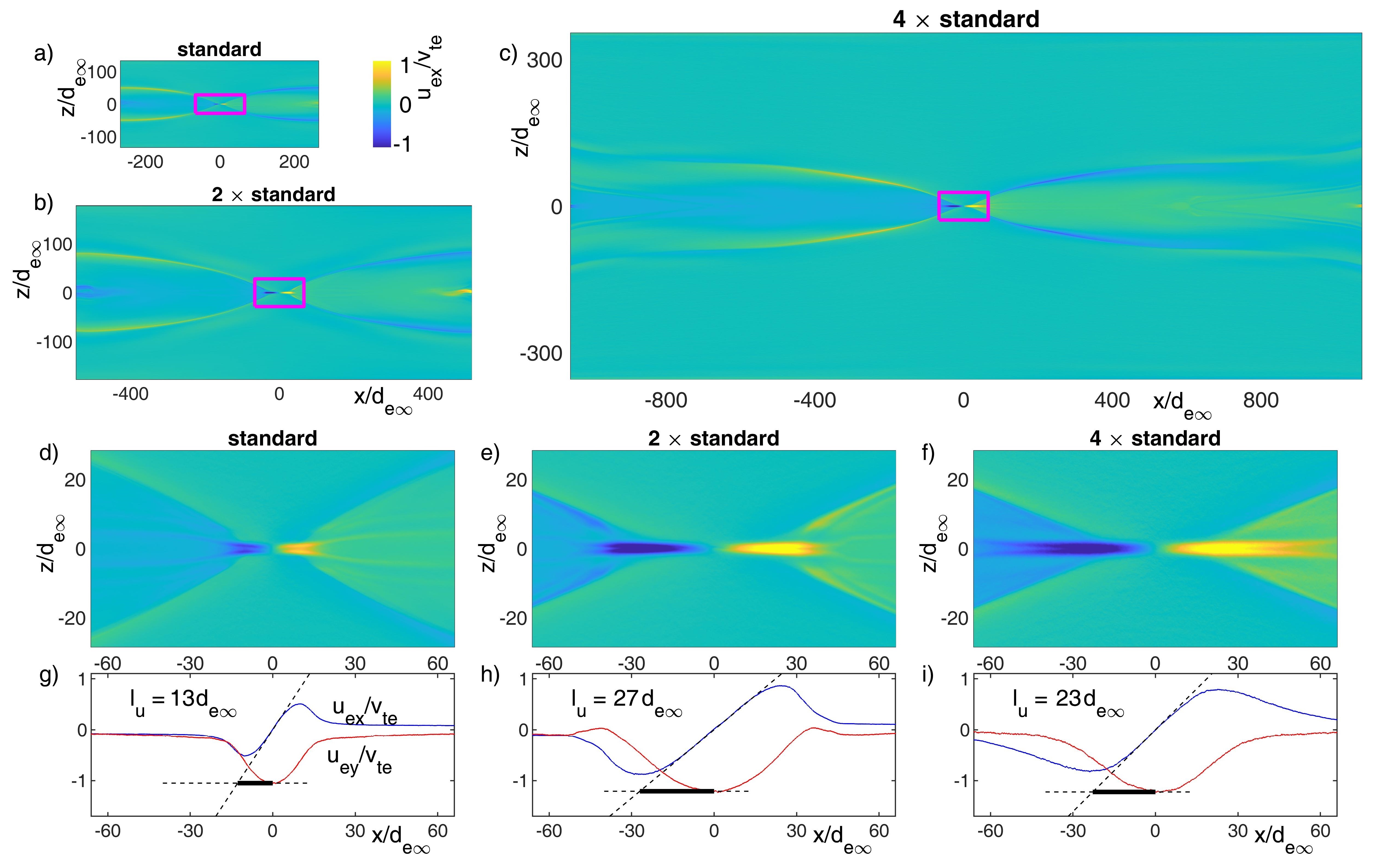
Figure 5: a-c) Profiles of $u_{ex}/v_{te}$ for the full simulation domains for three separate runs at $\beta_{e\infty}=2^{-4}$ and $m_{i}/m_{e}=800$. The run in a) has the “standard” size described in Section II.A, whereas the runs in b,c) are for simulations with spatial domain sizes increased by factors $2\times$ and $4\times$, respectively. Zoomed-in views of the EDRs are shown in d-f), whereas g-i) show cuts of $u_{ex}$ and $u_{ey}$ for $z=0$, from which the length scale $l_{u}$ of current layer rotation is determined.

IV Length scales of the EDR

We now introduce a new length $l_{u}$, which is a measure of the spatial scale at which the direction of the out-of-plane EDR electron current at the $X$-line rotates into the exhaust direction. This length scale turns out to be fundamental our momentum balance analysis of the EDR.

IV.1 Numerical evidence that $l_{u}$ does not scale with simulation system size

In Ref. Daughton, Scudder, and Homa (2006), which employed relatively low mass ratio $m_{i}/m_{e}=25$, it was observed that the length of the EDR increases with the size of the numerical simulation domain, and evidence was presented that the long electron current layers of the EDR could act as a bottleneck for reconnection. These results do not to apply to our present simulations where $m_{i}/m_{e}$ approaches its natural value of 1836. For example, in Fig. 5(a) profiles of $u_{ex}$ are shown for a simulation at $m_{i}/m_{e}=800$ and $\beta_{e\infty}=2^{-4}$ for the “standard” setup described in Section II.A, whereas Figs. 5(b,c) apply domains factors of $2\times$ and $4\times$ larger, respectively. Zoomed-in views of the EDRs for the three runs are shown in Figs. 5(d-f). In the standard case the length of the EDR is likely reduced due to the proximity of the simulation boundaries, whereas we notice how the $2\times$ and $4\times$ runs have longer EDR lengths. This indicates that for simulations at large $m_{i}/m_{e}$, the length of the EDR becomes independent of the system size when the run is implemented in a sufficiently large domain.

For the analytical analysis of the EDR the following definition of $l_{u}$ becomes essential to the presented theory for the force balance of the electron fluid. Here

$$l_{u}\equiv\left|\frac{u_{ey}}{du_{ex}/dx}\right|_{\mbox{\scriptsize X-line}},$$ (7)

represents a measure of the spatial distance that characterizes the rotation of the EDR electron current direction in the $xy$-plane as a function of $x$. Figs. 5(g-i) provide the geometric interpretation of this quantity, which is observed to be on the order of $20d_{e}$ for the three runs. Below we show how $l_{u}$ is significantly shorter than the full length $l_{\mbox{\scriptsize jet}}$ of the EDR for many runs in our study, consistent with previously observed two-scale EDR structures Karimabadi, Daughton, and Scudder (2007); Shay, Drake, and Swisdak (2007).

IV.2 Numerical results for $l_{u}$ over the full $(\beta_{e\infty},m_{i}/m_{e})$–matrix of kinetic runs

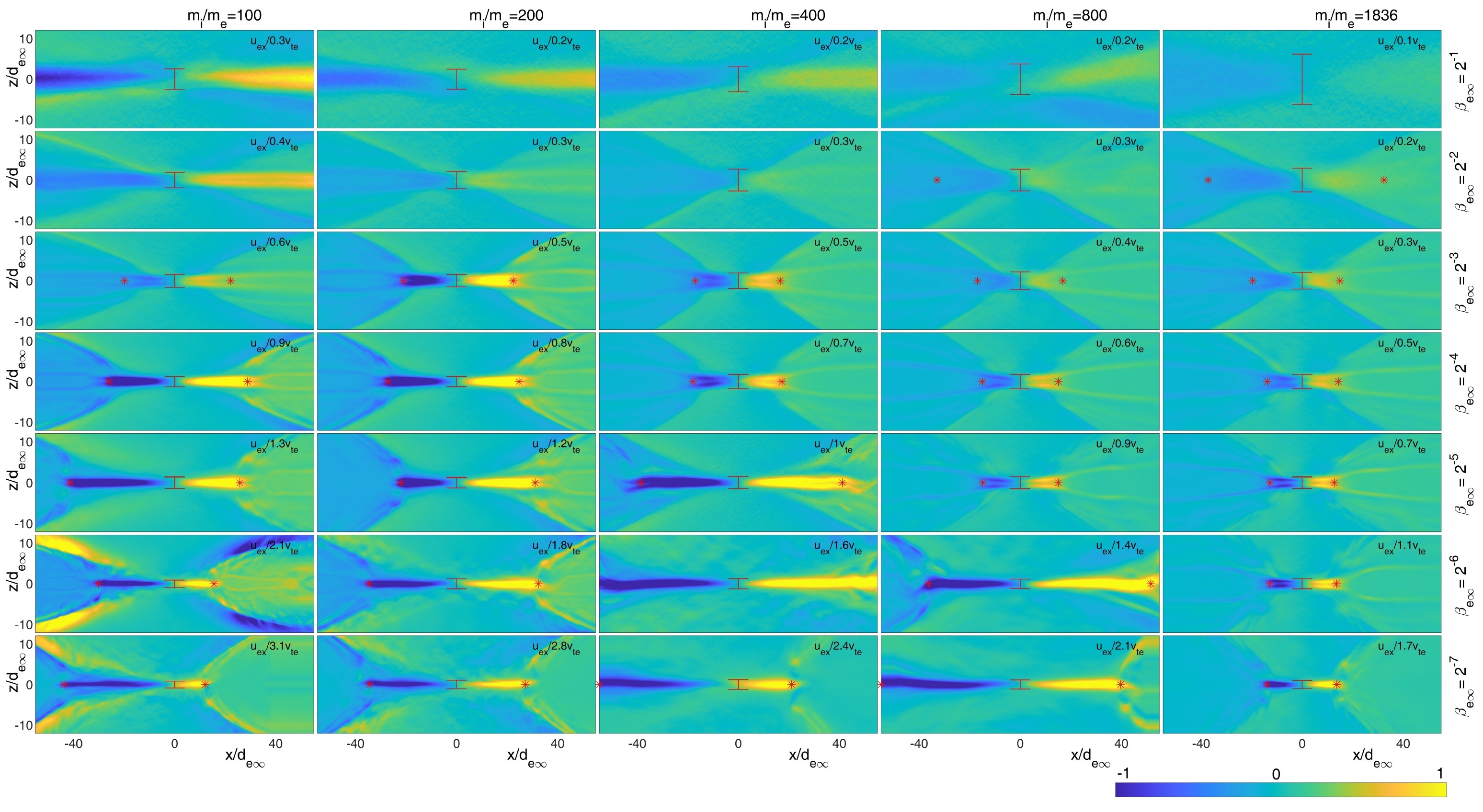
Figure 6: Color contours of $u_{ex}$ for the matrix of numerical simulations applied in the study, $m_{i}/m_{e}\in\{100,200,400,800,1836\}$ and $\beta_{e\infty}=2^{-k}$ with $k\in\{1,2,\dots,7\}$. When falling within the domains considered, the ends of the jets are marked by the red stars corresponding to $|u_{ex}|$ dropping to 60% of its peak value. The similarly defined width of the $u_{ey}$ out-of-plane electron drift is marked in each panel at $x=0$.

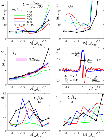
Figure 7: a,b) Recorded values of $l_{u}$ and $l_{\mbox{\scriptsize jet}}$, which are similar to the inner and outer lengths of the EDR introduced in Refs. Karimabadi, Daughton, and Scudder (2007); Shay, Drake, and Swisdak (2007). In b) the dashed lines indicate runs in the non-adiabatic regime with enhanced ${p_{e\parallel}}$-heating observed for $\beta_{e\infty}^{2}m_{i}/m_{e}\lesssim 1$. Evidently, this regime is also characterized by an enhancement in the length of the EDRs (while $l_{u}$ remains near constant). c) Half-width of the electron current layer, which approximately scales as 3.2 $\rho_{B_{H}}$. Here $\rho_{B_{H}}$ is the typical electron Larmor radius at the upstream edge of the EDR. d) Considering the run with $m_{i}/m_{e}=1836$ and $\beta_{e\infty}=2^{-4}$, the blue line is $-u_{ey}/v_{te}$, while the red line show the profile of $E_{z}$. The black line (full-width) indicates how $l_{z}$= half-width-half-maximum is obtained form $-u_{ey}/v_{te}$. e,f) Characteristic aspect ratios of the EDR, $l_{z}/l_{jet}$ and $l_{z}/l_{u}$, compared to the normalized reconnection rate $\alpha=E_{\mbox{\scriptsize rec}}/(v_{A}B)$.

Fig. 6 provides zoomed-in views of the EDRs recorded in the full set of runs applied in our study. As is typical for kinetic simulations of reconnection based on the Harris sheet geometry, after fast reconnection has commenced the reconnection rate initially increases and then reduces to a near steady state. Each of the profiles considered here correspond to times $t\simeq 70\Omega_{ci}^{-1}$ during these later intervals of mostly steady state reconnection geometries. For $\beta_{e\infty}\geq 2^{-2}$ elongated EDRs are mostly observed where $l_{\mbox{\scriptsize jet}}>100d_{e\infty}$. Here the out-of-plane electron flows are largely provided by the diamagnetic drifts similar to those of the Harris sheet. Meanwhile, for $\beta_{e\infty}\leq 2^{-3}$, the force balance condition of the EDR as expressed in Eq. (4) requires current densities boosted beyond those provided by the diamagnetic effect, and the EDRs acquire a shorter length. The marked ends of the jets are defined by the locations where $|u_{ex}|$ has fallen to 60% of its respective peak value. For the adiabatic regime ($\beta_{e\infty}^{2}m_{i}/m_{e}\gtrsim 1$), the lengths of the electron diffusion region are consistently observed to be $l_{\mbox{\scriptsize jet}}\simeq 20d_{e\infty}$. For the regime $\beta_{e\infty}^{2}m_{i}/m_{e}\lesssim 1$ of enhanced ${p_{e\parallel}}$ energization Egedal et al. (2015), a sharp transition occurs where the EDRs are characterized by longer outflow jets.

In Fig. 7 we show the values of $l_{u}$ and $l_{\mbox{\scriptsize jet}}$ for all the runs applied in the study. The runs with $\beta_{e\infty}\leq 2^{-3}$ (most relevant to the analysis in Section IV) are all characterized by $l_{u}\simeq 18d_{e\infty}$. In Fig. 7(b) the dashed lines represent runs in the aforementioned regime $\beta_{e\infty}^{2}m_{i}/m_{e}\lesssim 1$ of enhanced ${p_{e\parallel}}$ heating, and it is evident that this regime is characterized by larger values of $l_{\mbox{\scriptsize jet}}$.

IV.3 How continuity of electrons in the EDR sets the $l_{u}$ length scale

Directly related to ${\bf J}_{\mbox{\scriptsize extra}}$, we find that $l_{u}$ is shortened by the enhancement of the electron flow into the EDR. Let $u_{ey0}$ be the flow in the $y$-direction at the $X$-line; given the definition of $l_{u}$ the flow in the $x$-direction is then $u_{ex}=u_{ey0}x/l_{u}$. For a uniform inflow velocity $u_{ez}$ mass continuity requires that

$$nu_{ez}x=nu_{ex}l_{z}=nu_{ey0}xl_{z}/l_{u}$$

where $l_{z}$ is the half width of the EDR analysed below. Carrying on, it follows that

$$l_{u}=\frac{\displaystyle u_{ey0}l_{z}}{\displaystyle u_{ez}}=\frac{\displaystyle B_{H}}{\displaystyle en\mu_{0}u_{ez}}\quad.$$

Meanwhile, the strong parallel streaming of electrons in toward the EDR causes the inflow speed of the electrons to increase. Empirically we find

$$u_{ez}\simeq 3.5E_{\mbox{\scriptsize rec}}/B_{H}\quad.$$

This enhancement of the inflow speed above $E_{\mbox{\scriptsize rec}}/B_{H}$ is caused by the inflow pressure anisotropy through the term ${{\bf J}_{\perp}}_{\mbox{\scriptsize extra}}$, and is consistent with the profiles in Figs. 12(a,b).

As discussed above, the reconnection electric field, $E_{\mbox{\scriptsize rec}}$ adhere to the scaling laws of Ref. Shay et al. (2004) where

$$E_{\mbox{\scriptsize rec}}\simeq 0.1v_{A}B_{1di}=\frac{\displaystyle 0.1B_{1di}^{2}}{\displaystyle\sqrt{\mu_{0}nm_{i}}}\quad.$$

It then follows that

$$l_{u}\simeq\frac{\displaystyle B_{H}^{2}}{\displaystyle 0.35B_{1di}^{2}}\sqrt{\frac{\displaystyle m_{i}}{\displaystyle m_{e}}}d_{e}\quad.$$

Empirically and consistent with Fig. 1(a), the magnetic field 1$d_{i}$ upstream of the EDR is approximately $B_{1di}\simeq B_{\infty}/2$. Furthermore, due to non-adiabatic effects $B_{H}$ depends on $m_{i}/m_{e}$ (see Fig. 10(a)), and the scaling is consistent with $B_{H}^{2}\sqrt{m_{i}/m_{e}}/(0.35B_{1di}^{2})\simeq 17$ for all the runs. This scaling is also in agreement with recent results in Ref. Liu et al. (2022). In turn, this is in reasonable agreement with the observation that $l_{u}\simeq 18d_{e\infty}$ in Fig. 7(a). It should be noted that $l_{u}$ varies within the duration of a single simulation, but its precise length does not impact the qualitative predictions of the theory being presented below.

IV.4 The half-width, $l_{z}$, of the EDR

The width of the EDR has previously been determined to scale with the orbit width of the meandering electrons Horiuchi and Sato (1997); Shay and Drake (1998); Roytershteyn et al. (2013); that result is also consistent with the simulations presented here. In Fig. 7(c), the half-width $l_{z}$ is shown for each of the simulations. As illustrated in Fig. 7(d), we define $l_{z}$ as the half-width where the half-maximum of the electron $u_{ey}$ flow velocity is recorded for $x=0$. We note that the simple approximation $l_{z}\simeq 2d_{e\infty}$ represents a reasonable estimate; this is especially true for the normalized electron pressures most typical in the Earth’s magnetotail, $\beta_{e\infty}\simeq 0.1$.

More accurately, the meandering orbit width of the electrons is related to the electron Larmor radius at the upstream edge of the EDR, $\rho_{B_{H}}=\sqrt{2m_{e}T_{e\perp}}/(eB)$, and can be estimated using $B=B_{H}$ in Eq. (4), and $T_{e\perp}=T_{e\infty}B_{H}/B_{\infty}$. Thus, we then find

$$\rho_{B_{H}}=d_{e\infty}\left(\frac{\displaystyle B_{\infty}}{\displaystyle B_{H}}\beta_{e\infty}\right)^{\frac{1}{2}}=d_{e\infty}\left(\frac{\displaystyle 12}{\displaystyle\pi}\right)^{\frac{1}{8}}\beta_{e\infty}^{\frac{1}{4}}\quad.$$ (8)

The thick magenta line in Fig. 7(c) represents $3.2\rho_{B_{H}}$ and provides a good approximation for $l_{z}$ for the runs at $\beta_{e\infty}\leq 2^{-2}$ and $m_{i}/m_{e}\geq 400$. At the lowest values considered for $\beta_{e\infty}$, however, its is observed that $3.2\rho_{B_{H}}$ underestimates $l_{z}$. This slightly weaker scaling of $l_{z}$ as a function of $\beta_{e\infty}$ may in part be explained by the fact that a fraction of the $u_{ey}$-drift is caused by the $E\times B$-drift of the strong $E_{z}$ field at the upstream edge of the EDR. This field is illustrated by the red line in Fig. 7(d) and the color profile in Fig. 8(a); for all the runs we find that the width of this $E_{z}$-structure is fixed when normalized by $d_{e\infty}$ (not shown).

Due to the strong drift provided by ${\bf J}_{\mbox{\scriptsize extra}}$ and because the currents inside the EDR are being driven by ${p_{e\parallel}}-{p_{e\perp}}$, it is not mathmatically guaranteed that the aspect ratio of the EDR is directly related to the normalized reconnection rate $\alpha$ discussed above and shown in Fig. 2(a). Therefore, in Figs. 7(e,f) we show the recorded values of $l_{z}/l_{jet}$ and $l_{z}/l_{u}$ both normalized by $\alpha$. In particular, it is observed that $(l_{z}/l_{u})\simeq\alpha$ for most of the runs with $m_{i}/m_{e}\geq 400$. This quantity may then be useful for estimating the normalized reconnection rate from spacecraft observations Burch et al. (2020).

V Breaking the frozen-in law at the reconnection $X$-line

The major force terms of the EDR are ${\bf J}\times{\bf B}$ and $\nabla\cdot{\bf p}_{e}$ which largely balance. As discussed above this force balance requirement can ultimately be expressed through the conditions in Eqs. (2) or (4). However, as seen in Fig. 3(a), in a small region ($4d_{e}\times 2d_{e}$) centered on the $X$-line the $({\bf J}\times{\bf B})_{y}$ force vanishes, such that the more detailed force balance right at the $X$-line then requires that the RHS of Eq. (6) also vanishes (consistent with Fig. 3(b)). Thus, for the considered anti-parallel and symmetric configurations and within this limited region around the $X$-line, the force balance constraint of Eq. (1) only involves the off-diagonal stress in the electron pressure tensor Cai, Ding, and Lee (1994):

$$E_{\mbox{\scriptsize rec}}=-\frac{1}{en}\left(\frac{\displaystyle\partial p_{exy}}{\displaystyle\partial x}+\frac{\displaystyle\partial p_{eyz}}{\displaystyle\partial z}\right)\quad.$$ (9)

Again, here $E_{\mbox{\scriptsize rec}}$ is the $E_{y}$ electric field along the $X$-line (that is aligned with the $y$ axis and runs through $(x,z)=(0,0)$). By Faraday’s law $E_{\mbox{\scriptsize rec}}$ then represents the rate at which magnetic flux crosses the $X$-line. Below we will derive a new model for the terms in Eq. (9), providing a theory consistent with fast reconnection controlled by larger scale dynamics external to the EDR.

V.1 Meandering orbit motion of electrons within the EDR, setting the striated structure of the electron distribution function

To elucidate how the upstream electron pressure anisotropy drives the current of the EDR, in Fig. 8 we consider the trajectories of electrons with field-aligned velocities ${\bf v}=3.3v_{te}{\bf B}/B$ injected with $z=-4d_{e\infty}$ at various values of $x<0$ just upstream of the EDR. Here $v_{te}=\sqrt{T_{e}/m_{e}}$ is the electron thermal speed. The trajectories, computed through integration of the equations of motion with a Matlab ODE solver in the simulation fields, are representative because the upstream distributions (like in Figs. 9(a,d)) with ${p_{e\parallel}^{\mbox{\scriptsize edge}}}\gg{p_{e\perp}^{\mbox{\scriptsize edge}}}$ “feed” electrons to the EDR with $|v_{\parallel}|\gg{v_{\perp}}$ Ng et al. (2011). In Figs. 8(a,b) the parts of the trajectories with $z<0$ ($z>0$) are represented by the blue (red) full lines. To better illustrate the orbit morphology, for each transit across $z=0$ in Fig. 8(b) additional orbits are initialized and shown by the dashed lines. This visualizes how the average force of $-e{\bf v}\times B_{z}{\bf e}_{z}$ causes the meandering Speiser-type motion Speiser (1965) to diverge away from the $X$-line.

The EDR current is caused in part by the $E\times B$-drift of the $E_{z}$ field displayed in Fig. 8(a). The large values of $E_{z}$ are consistent with momentum balance with the strong gradients of $p_{\|}$ at the interface of the EDR. The initial blue section of the trajectories in Fig. 8(b) are aligned with the magnetic field at the upstream edge of the EDR. Thus, the direction of the parallel thermal streaming is sensitive to the $B_{y}$ Hall magnetic field, which thereby sets the angle in the $xy$-plane at which the electrons are injected into the EDR region.

In Figs. 8(c-e) the colored and encircled triangles represent the particle velocities corresponding to the similarly colored velocity vectors in Fig. 8(b). For example, the magenta vector at $x=0$ in Fig. 8(b) pointing mostly in the $x$-direction, yields the velocity of an electron reaching the $X$-line directly from the upstream region, and the corresponding encircled magenta triangle in Fig. 8(d) has $|v_{x}|\gg|v_{y}|$. The $X$-line may also be reached through multiple meandering motions within the layer, steadily directing the velocity into the $-y$-direction. As shown in Figs. 8(c-e), repeating this procedure for four more initial velocities ${\bf v}=v_{\parallel}{\bf B}/B$ within the interval $0.1\leq v_{\parallel}/v_{te}\leq 3.3$ yields the lines of colored triangles, corresponding to the centers of the striated structures of the EDR electron distributions first described in Ref. Ng et al. (2011). In Figs. 8(c-e), the similar points marked by green circles are the result of injecting electrons along field lines from the opposing inflows of the EDR. Also, going from $x/d_{e\infty}=-3$ to $x/d_{e\infty}=3$, we note how the displayed structures rotates in the $v_{x}v_{y}$-plane (and similarly in Fig. 9), corresponding to the rotation of the EDR current layer direction mentioned above Ng et al. (2011); Shuster et al. (2015), and parameterized by $l_{u}$.

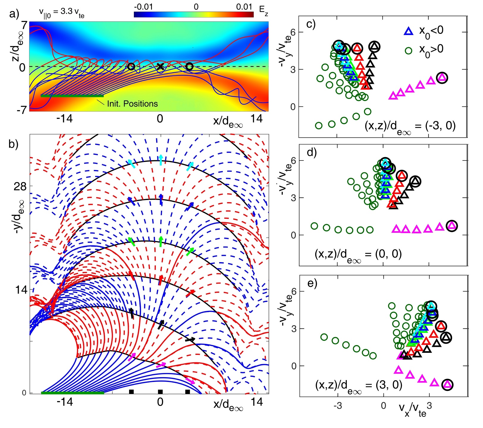
Figure 8: a,b) Trajectories of electrons injected along field lines into the EDR with $v_{\parallel}=3.3v_{te}$. Three points, $(x,z/d_{e\infty})=(-3,0);(0,0);(3,0)$, are selected in a) indicating the spatial locations where the velocity arrows in b) are evaluated. As indicated, the panels c-e) also correspond to these locations. The angles indicated by arrows in b) at which the trajectories reach the selected points, determine the location of the encircled triangles in c), d), and e), respectively. Similar trajectories are obtained by using a range of initial $v_{\parallel}$ values and result in the striated structures marked by the symbols in c), characteristic of the EDR distributions Ng et al. (2011) and observed in Fig. 9.

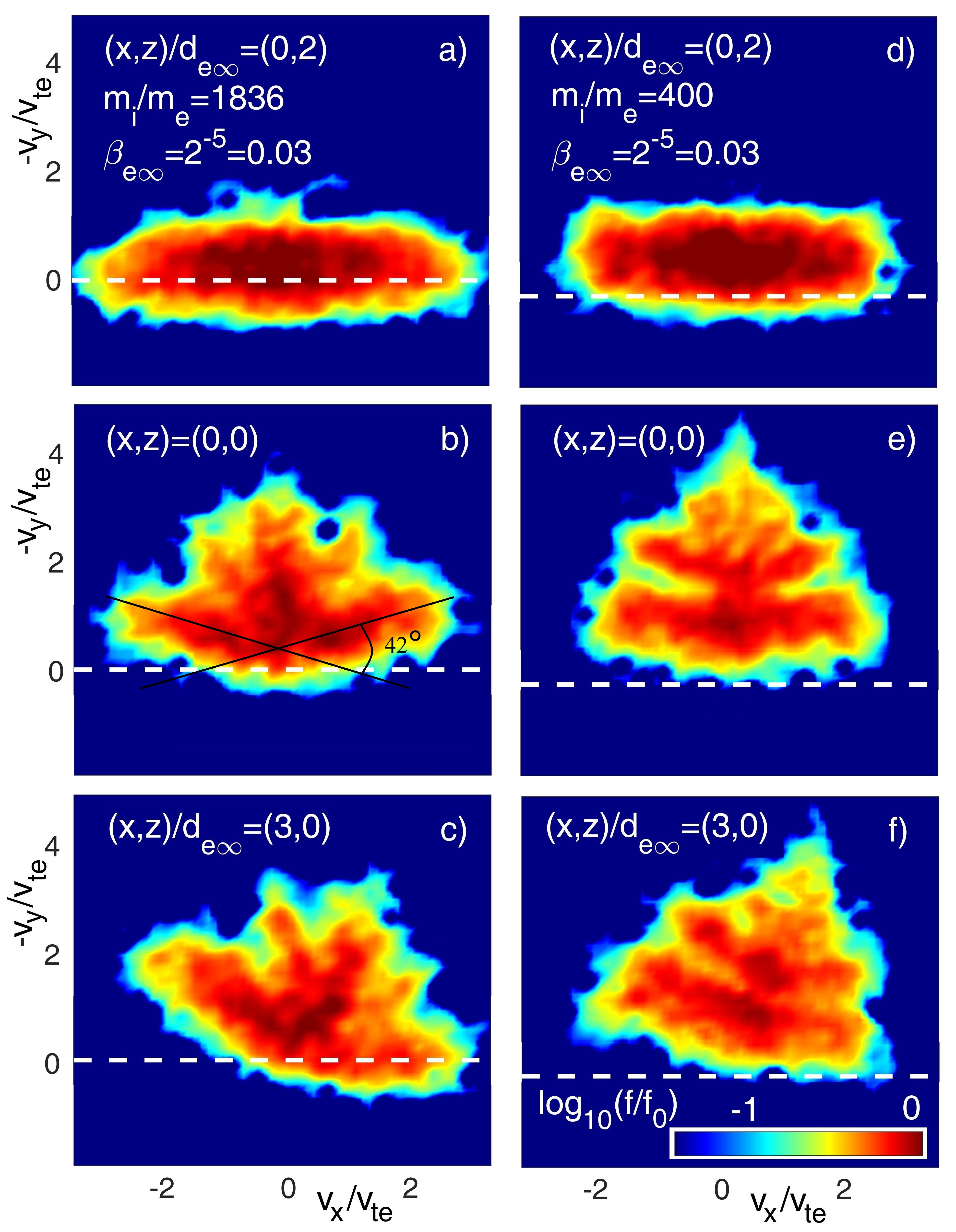
Figure 9: Projections, $f_{xy}(v_{x},v_{y})=\int f({\bf v})dv_{z}$ of EDR electron distributions, recorded in simulations for $m_{i}/m_{e}=1836$ in a-c) and $m_{i}/m_{e}=400$ in d-f). The differences between the profiles are consistent with enhanced $\Delta p_{eyy,E}$ for $m_{i}/m_{e}=400$, caused by $\hat{E}_{\mbox{\scriptsize rec,400}}\simeq 2\hat{E}_{\mbox{\scriptsize rec,1836}}$.

V.2 Origin for the off-diagonal $\partial p_{exy}/\partial x$-stress at the reconnection $X$-line

To understand how the upstream pressure anisotropy influences $p_{exy}$ we consider the electron distributions in Fig. 9. At the upstream edge of the EDR we have $p_{eyy}\simeq p_{ezz}$, and given Eq. (3) it follows that $p_{eyy}-p_{exx}=-{\Delta p_{e\|\perp}^{\mbox{\scriptsize max}}}$. Comparing the distributions in Figs. 9(a,b)) it is clear that only a fraction of this upstream anisotropy is carried by the orbit motion to the $X$-line. Empirically at the $X$-line we find that

$$\left.\left(p_{eyy}-p_{exx}\right)\right|_{\mbox{\scriptsize X-line}}=-\dfrac{4}{5}{\Delta p_{e\|\perp}^{\mbox{\scriptsize max}}}+\Delta p_{eyy,E}\quad.$$ (10)

The lines in Fig. 9(b)) are drawn in “by eye” to indicate the center line of the striations in the $(v_{x},v_{y})$-plane, corresponding to electrons reaching the X-line without bounces across $z=0$. The factor of $4/5$ can be understood by noting the $\sim 42^{\circ}$ angle between these lines, which is double the angle at which the electrons are launched (by the ratio of $B_{y}/B_{x}$) as they initially enter the EDR. The change in the straight distribution just upstream of the EDR (with ${\Delta p_{e\|\perp}^{\mbox{\scriptsize max}}}$) into the distribution with each side “bent in the middle” by $21^{\circ}$ then yields a simple estimate for the relative reduction in $p_{exx}-p_{eyy}$:

$$\frac{\displaystyle\left.\left(p_{exx}-p_{eyy}\right)\right|_{\mbox{\scriptsize X-line}}}{\displaystyle{\Delta p_{e\|\perp}^{\mbox{\scriptsize max}}}}=\cos^{2}(21^{\circ})-\sin^{2}(21^{\circ})/4\simeq 0.84\quad.$$

The phase space density of the striations for the higher bounce numbers mainly add to $p_{eyy}$, explaining the further reduction in the ratio towards $4/5$.

The additional term, $\Delta p_{eyy,E}$, in Eq. (10) corresponds to an increase in $p_{eyy}$ due to direct heating of electrons by the reconnection electric field. From Fig. 8 it is clear that the “tips” of the triangular shaped distributions are composed of electrons meandering multiple times while streaming mostly in the $-y$-direction, energized most significantly by $\hat{E}_{\mbox{\scriptsize rec}}$. The more pronounced triangular shapes in Figs. 9(e,f) compared to Figs. 9(b,c) are consistent with stronger $\Delta p_{eyy,E}$ heating, as the value of $\hat{E}_{\mbox{\scriptsize rec}}$ for $m_{i}/m_{e}=400$ is about twice as large compared to that observed in the $m_{i}/m_{e}=1836$ run.

As detailed with Figs. 8 and 9, within the EDR the $xy$-projections of the electron distributions rotate approximately as a “solid-body” Ng et al. (2011); Divin et al. (2016) such that for small $x/l_{u}$

$$p_{exy}=\frac{x}{l_{u}}\left.\left(p_{eyy}-p_{exx}\right)\right|_{\mbox{\scriptsize X-line}}\quad.$$ (11)

Combining Eqs. (10) and (11) we then obtain

$$\frac{\displaystyle\partial p_{exy}}{\displaystyle\partial x}=\frac{1}{l_{u}}\left(-\dfrac{4}{5}{\Delta p_{e\|\perp}^{\mbox{\scriptsize max}}}+\Delta p_{eyy,E}\right)\quad.$$ (12)

V.3 Origin for the off-diagonal $\partial p_{eyz}/\partial z$-stress at the reconnection $X$-line

In the present paper we do not provide a formal derivation of the $\partial p_{eyz}/\partial z$-stress. However, the first term in Eq. (12) is independent of $E_{\mbox{\scriptsize rec}}$ as it is imposed by the upstream pressure anisotropy. The motion of each electron in the X-line region is naturally governed by Newton’s laws, and once all forces are summed up over the electrons in a fluid element, the terms independent of $E_{\mbox{\scriptsize rec}}$ must cancel in order for the fluid to be in force balance. Thus, force balance at the X-line requires that the $\partial p_{exy}/\partial x$ stress imposed externally is cancelled by an opposite term in Eq. (9). The only term available for this cancellation is $\partial p_{eyz}/\partial z$, and this simple argument then suggests that

$$\frac{\displaystyle\partial p_{eyz}}{\displaystyle\partial z}=\frac{1}{l_{u}}\dfrac{4}{5}{\Delta p_{e\|\perp}^{\mbox{\scriptsize max}}}\quad.$$ (13)

Some theoretical support for Eq. (13) can be derived from the results in Refs. Kuznetsova, Hesse, and Winske (1998); Hesse et al. (1999), which also obtained approximations for the off-diagonal pressure tensor derivatives ($\partial p_{exy}^{\mbox{\scriptsize Hesse}}/\partial x$ and $\partial p_{eyz}^{\mbox{\scriptsize Hesse}}/\partial z$).

$$\frac{\displaystyle\partial p_{exy}^{\mbox{\scriptsize Hesse}}}{\displaystyle\partial x}=\frac{\displaystyle\partial p_{eyz}^{\mbox{\scriptsize Hesse}}}{\displaystyle\partial z}=n\sqrt{\frac{\displaystyle m_{e}T_{e}}{\displaystyle 2}}\,\frac{\displaystyle\partial u_{ex}}{\displaystyle\partial x}\quad.$$

These were derived through an assumption of isotropic upstream electron pressure. As such, given that upstream of the EDR $p_{exx}-p_{eyy}=\Delta p_{\|,\perp}$ is large, the $\partial p_{exy}^{\mbox{\scriptsize Hesse}}/\partial x$-approximation is inaccurate and is not consistent with the simulation data presented below. In contrast, the conditions required for the accuracy of $\partial p_{eyz}^{\mbox{\scriptsize Hesse}}/\partial z$ are well satisfied, as the upstream pressure in the $yz$-plane is isotropic, $p_{eyy}\simeq p_{ezz}\simeq{p_{e\perp}^{\mbox{\scriptsize edge}}}$. Still, we find that a scale-factor must be applied, $\partial p_{eyz}/\partial z\simeq 3.6\,\partial p_{eyz}^{\mbox{\scriptsize Hesse}}/\partial z$, for matching our numerical results at $m_{i}/m_{e}=1836$ and $\beta_{e\infty}\leq 2^{-4}$ (see below).

Using the result above that the width of the EDR is $l_{z}\simeq 3.2\rho_{B_{H}}$, from Ampère’s law it follows that $u_{e}=B_{H}/(\mu_{0}enl_{z})=B_{H}^{2}/(3.2\,\mu_{0}nm_{e}{v_{\perp}})$. With $\partial u_{ex}/\partial x=u_{e}/l_{u}$, and following Refs. Kuznetsova, Hesse, and Winske (1998); Hesse et al. (1999) we find

$$\frac{\displaystyle\partial p_{eyz}}{\displaystyle\partial z} \simeq 3.6\frac{\displaystyle\partial p_{eyz}^{\mbox{\scriptsize Hesse}}}{\displaystyle\partial z}\simeq\frac{\displaystyle 3.6}{\displaystyle 3.2}\sqrt{\frac{m_{e}T_{e\perp}}{2}}\frac{B_{H}^{2}}{\mu_{0}m_{e}{v_{\perp}}l_{u}}$$ (14)

$$\simeq \frac{\displaystyle 9}{\displaystyle 16}\frac{B_{H}^{2}}{\mu_{0}l_{u}}\simeq 0.804\frac{{\Delta p_{e\|\perp}^{\mbox{\scriptsize max}}}}{l_{u}}\simeq\frac{4}{5}\frac{{\Delta p_{e\|\perp}^{\mbox{\scriptsize max}}}}{l_{u}}\,\,.$$

As illustrated by the black contours in Figs. 1(c), for the present configurations the momentum balance in Eq. (4) corresponds to the condition $0.7B_{H}^{2}/\mu_{0}\simeq{\Delta p_{e\|\perp}^{\mbox{\scriptsize max}}}$. This substitution was applied in the last line of Eq. (14). Below we will show how the scale factor of 3.6 in front of $\partial p_{eyz}^{\mbox{\scriptsize Hesse}}/\partial z$ is supported by the numerical data obtained at $m_{i}/m_{e}=1836$, $\beta_{e\infty}\leq 2^{-4}$ (see Fig. 11(a)), and its theoretical origin will be the subject of further investigations.

V.4 The term breaking the electron frozen in law

Given the described cancellation of terms, the theory suggests that the electron dynamics of the EDR do not represent a bottleneck for reconnection. Again, inserting Eqs. (12) and (13) into Eq. (9) only one term remains for balancing the reconnection electric field

$$E_{\mbox{\scriptsize rec}}\simeq-\frac{1}{enl_{u}}\Delta p_{eyy,E}\quad.$$ (15)

Separate from the force balance constraint expressed in Eq. (15) we can obtain a second independent estimate for $\Delta p_{eyy,E}$: In Fig. 8 we observe that electrons in the $X$-line region typically travel a distance between $0$ and 2$l_{u}$ in the $y$-direction such that $\Delta p_{eyy,E}\simeq-enl_{u}E_{\mbox{\scriptsize rec}}$. Applying this in Eq. (15) we obtain the seemingly mundane expression that

$$E_{\mbox{\scriptsize rec}}\simeq E_{\mbox{\scriptsize rec}}\quad.$$ (16)

Nevertheless, this is an important result, as it shows that the present geometry can accommodate any reconnection rate imposed at larger scales onto the EDR region. This is consistent with the near-uniform “ion-normalized-reconnection” rate, $\alpha$, in Fig. 2(a). It also confirms previous numerical results and theoretical conjectures that, with the formation of electron scale current layers, the electron dynamics can readily accommodate the rates of reconnection imposed by the plasma behavior at larger scales Shay et al. (1999); Stanier et al. (2015); Liu et al. (2017). We also note that because $E_{\mbox{\scriptsize rec}}\propto\Delta p_{eyy,E}/l_{u}$ and $\Delta p_{eyy,E}\propto l_{u}$, the reconnection rate becomes independent of $l_{u}$. In Appendix C we include additional discussion of how our interpretation of Eqs. (15) and (16) are not in conflict with results of resistive fluid models.

V.5 Numerical evidence for the validity of the model

As described above, the theory is aided by fully kinetic VPIC simulations carried out for a matrix of $\beta_{e\infty}$ and $m_{i}/m_{e}$ values. We next validate each of the separate theoretical predictions against the numerical results. First, the described dynamics involving trapped electrons require that within the inflow regions $|u_{e\|}|\ll v_{te}$, which is valid for $\beta_{e\infty}\gtrsim\sqrt{m_{e}/m_{i}}$ Egedal et al. (2015); Le et al. (2015), and the predicted profiles $B_{H}$ are confirmed in Figs. 10(a).

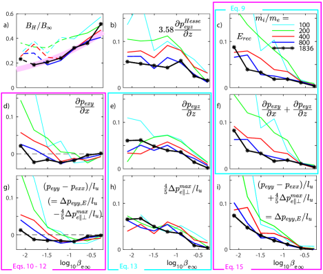
Figure 10: Obtained from a matrix of 35 kinetic simulations, profiles as functions of $\log_{10}(\beta_{e\infty})$ are shown for a range of parameters as marked in the panels. In a) the magenta line is Eq. (4). In c) $E_{\mbox{\scriptsize rec}}$ is normalized by $T_{e\infty}/(ed_{e0})$ (which is different from $\hat{E}_{\mbox{\scriptsize rec}}$ in Fig. 2(b)). The profiles in b), d–i) are various electron pressure tensor derivatives, normalized by $-n_{\times}T_{e\infty}/(ed_{e0})$, such that the resulting dimensionless values can be compared directly to those of $E_{\mbox{\scriptsize rec}}$ in c).

For all the numerical runs in our study, the individual contributions of $\partial p_{exy}/\partial x$ and $\partial p_{eyz}/\partial z$ are shown in Figs. 10(d,e), respectively. In Fig. 10, ${E}_{\mbox{\scriptsize rec}}$ is normalized by $T_{e}/(ed_{e0})=0.024$, and for direct comparison, all terms involving pressure derivatives are normalized by $-n_{e\times}T_{e\infty}/d_{e0}$. With this normalization, confirming Eq. (9), the sum of $\partial p_{exy}/\partial x+\partial p_{eyz}/\partial z$ in Fig. 10(f) reproduces with good accuracy $E_{\mbox{\scriptsize rec}}$ in Fig. 10(c).

Eqs. (10)-(12) represent a key insight for the theory which is confirmed numerically, as Fig. 10(g) provides an accurate representation of Fig. 10(d). Consistent with recent spacecraft observations Egedal et al. (2019), $\partial p_{exy}/\partial x$ is mostly negative for runs with $m_{i}/m_{e}\geq 400$, and is thus dominated by the external stress imposed by ${p_{e\parallel}^{\mbox{\scriptsize edge}}}\gg{p_{e\perp}^{\mbox{\scriptsize edge}}}$. Likewise, Eq. (13) is supported by the data, as the profiles of $\frac{4}{5}{\Delta p_{e\|\perp}^{\mbox{\scriptsize max}}}/l_{u}$ in Fig. 10(h), are observed to provide a match to $\partial p_{eyz}/\partial z$ in Fig. 10(e). This is especially the case for $m_{i}/m_{e}\geq 400$, corresponding to the adiabatic limit required for the validity of Eq. (4). Also in this limit, the sums shown in Fig. 10(i) of the profiles of Figs. 10(g,h) provide a good match to $E_{\mbox{\scriptsize rec}}$ in Fig. 10(c), confirming Eq. (15).

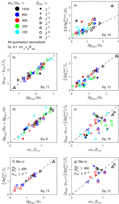
Figure 11: As indicated in the panels of a-g), the LHS and RHS of key equations of the manuscript are tested using data collected in the numerical runs. Most significantly, in b) Eq. (11) is confirmed, and in f) Eq. (13) is confirmed for the important parameter range of $m_{i}/m_{e}\geq 400$ and $\beta_{e\infty}\leq 2^{-3}$. To ensure that data from the runs with the largest values of $\beta_{e\infty}$ do not cluster close to $(0,0)$, all terms are normalized by $0.1en_{e\times}v_{A}B_{up}$.

To further validate the most important equations in the study, in Fig. 11 we plot the terms of Eqs. (9), (11), (13), (14), and (15), with all the shown quantities normalized by $0.1en_{e\times}v_{A}B_{up}$. First, in panel a) the factor of $\sim 3.6$ used in Eq. (14) is consistent with the data at $m_{i}/m_{e}=1836$, $\beta_{e\infty}\leq 2^{-4}$. In panels b) and c) the approximations introduced for $\partial p_{exy}/\partial x$ and $\partial p_{eyz}/\partial z$ are validated. For the case of $\partial p_{eyz}/\partial z$ panel f) indicates an improved accuracy of the approximation for the most relevant parameters of $m_{i}/m_{e}\geq 400$ and $\beta_{e\infty}\leq 2^{-3}$. From panel d) it is clear that the momentum balance Eq. (9) is well satisfied by the simulations. Panel e) tests the penultimate expression (Eq. (15)) of the paper. Because of the often opposing signs of the $\partial p_{exy}/\partial x$ and $\partial p_{eyz}/\partial z$ estimates, when calculating their sum the relative uncertainty/error is enhanced, explaining the enhanced scatter of the data points. However, as shown in panel g), when limiting the simulations to those with $m_{i}/m_{e}\geq 400$ and $\beta_{e\infty}\leq 2^{-3}$ most predictions for $E_{\mbox{\scriptsize rec}}$ fall within 20% of the correct value and all predictions are within 50%.

VI Summary and discussion

The use of the VPIC code implemented in a modern super-computing facility enabled a matrix of simulations to be performed for anti-parallel magnetic reconnection. This matrix spans a range of the normalized electron pressures, $\beta_{e\infty}$, as well as the ion to electron mass ratios, $m_{i}/m_{e}$. Our study reveals a range of results, which require new interpretations of the electron dynamics of the EDR and inner IDR that are different from previous models including those in Refs. Hesse et al. (1999); Drake, Shay, and Swisdak (2008); Daughton, Scudder, and Homa (2006). A main difference from the numerical studies a decade or more ago is our recent ability to carry out routine kinetic simulations at the natural proton to electron mass ratio of $m_{i}/m_{e}=1836$. At full mass ratio the effect of the electron pressure anisotropy that develops in the reconnection inflow becomes the dominant force-term not only within the EDR but also for the inner part of the IDR.

It has previously been determined Le et al. (2009); Egedal, Le, and Daughton (2013) that upstream of the EDR strong electron pressure anisotropy with $p_{e\|}\gg p_{e\perp}$ is driven by the convection of electrons into the reconnection region characterized by low values of $B$. This upstream pressure anisotropy is responsible for driving the strong electron currents within the EDR. In addition, with Fig. 3 we visualize how the electron inflow speed for locations inside the IDR (but outside the traditional EDR) exceeds the inflow speed of the magnetic field by a factor up to 3.5. This enhances the Hall magnetic field perturbation beyond what can be expected from traditional “whistler reconnection” Drake, Shay, and Swisdak (2008). Nevertheless, it is still possible that the condition $({\bf J}\times{\bf B})_{y}\simeq(\nabla\cdot{\bf p}_{e})_{y}$ is compatible with dispersive waves Rogers et al. (2001); Cassak et al. (2015). The strong Hall field $B_{y}$ perturbations at the edge of the EDR are mainly a consequence of dynamics related to the electron pressure anisotropy yielding a new and dominate force balance constraint, namely $({\bf J}\times{\bf B})_{y}\simeq(\nabla\cdot{\bf p}_{e})_{y}\gg en_{e}E_{\mbox{\scriptsize rec}}$. Furthermore, the enhanced perpendicular flow into the EDR by ${\bf J}_{\mbox{\scriptsize extra}}=[({p_{e\parallel}}-{p_{e\perp}})/B]{\bf b}\times\mathbf{\kappa}$ must be sourced by electrons flowing along the field lines on the inflow-side of the separatrix layers. This is consistent with spacecraft observations that the Hall currents extend many tens of $d_{i}$ away from the EDR Manapat et al. (2006).

Aside from the results summarized above, the main goal of this paper is to develop a theory that can account for the electron momentum balance directly at the $X$-line within the center of the EDR for anti-parallel reconnection. Previously, Refs. Kuznetsova, Hesse, and Winske (1998); Hesse et al. (1999) provided approximate expressions for the off-diagonal stress terms $\partial p_{exy}/\partial x$ and $\partial p_{eyz}/\partial z$. After applying a scale factor, their theoretical form for $\partial p_{eyz}/\partial z$ is in agreement with our numerical results. Meanwhile, the electron pressure anisotropy that develops upstream of the EDR turns out to have a large impact on $\partial p_{exy}/\partial x$ not previously considered. Our updated theory for $\partial p_{exy}/\partial x$ is cast in two separate terms. The first term is caused by the upstream electron pressure anisotropy and cancels the stress of $\partial p_{eyz}/\partial z$. In hindsight, this cancellation is not surprising as the EDR current, mainly driven by the upstream $p_{e\|}\gg p_{e\perp}$, must be in force balance independent of the value of $E_{\mbox{\scriptsize rec}}$.

The additional second term for $\partial p_{exy}/\partial x$ in Eq. (12) is the term that scales with $E_{\mbox{\scriptsize rec}}$ and as such, can be considered the term that actually breaks the electron frozen-in condition at the $X$-line. This term is related to the increase of the $p_{eyy}$ pressure tensor element caused directly through heating by $E_{\mbox{\scriptsize rec}}$. Because the electron flow in the $y$-direction is largely fixed by the upstream $p_{e\|}\gg p_{e\perp}$ (see Eq. (4)), the increase in $p_{eyy}$ becomes linear in $E_{\mbox{\scriptsize rec}}$, and the rotation with length scale $l_{u}$ of $p_{eyy}$ in the $xy$-plane then yields the stress required to balance $E_{\mbox{\scriptsize rec}}$. Because the term is proportional to $E_{\mbox{\scriptsize rec}}$, it facilitates reconnection at any external rate imposed onto the EDR. From the perspective of the electrons the reconnection rate is $\hat{E}_{\mbox{\scriptsize rec}}$ shown in Fig. 10(c), and runs with low values of $m_{i}/m_{e}$ have significant enhanced values of $\hat{E}_{\mbox{\scriptsize rec}}$. Even so, the identified reconnection mechanism can still accommodate these artificially enhanced values of $\hat{E}_{\mbox{\scriptsize rec}}$.

In closing, we note that our new theory predicts that $\partial p_{exy}/\partial x$ and $\partial p_{eyz}/\partial z$ have opposite signs for $m_{i}/m_{e}=1836$. This result has been directly confirmed in spacecraft observations of an EDR encounter by MMS in the Earth’s magnetotail Egedal et al. (2019). Other MMS observations also support the approximation that reconnection in the Earth’s magnetotail occurs in regimes consistent with laminar 2D kinetic models. One reason for the apparent success of such laminar 2D models is perhaps that for $m_{i}/m_{e}=1836$ the force by $E_{\mbox{\scriptsize rec}}$ is small compared to the forces associated with electron pressure anisotropy, such that $E_{\mbox{\scriptsize rec}}$ only slightly perturbs the electron orbit dynamics within the EDR. Again, from the perspective of the electrons the reconnection rates imposed by the inertia and dynamics of the much heavier ions are in fact very modest and the small modifications imposed by $E_{\mbox{\scriptsize rec}}$ on the electron motion is not sufficient to drive strong instabilities. In order for instabilities to alter the momentum equation in Eq. (1) they much have an inverse growth rate similar to the short electron transit time through the EDR. For example, the Lower-Hybrid-Drift-Instability (LHDI) may perturb the out-of-plane structure of the EDR, but this does not necessarily cause a fundamental change in its underlying 2D dynamics Le et al. (2017); Greess et al. (2021); Schroeder et al. (2022). Given recent progress in the understanding of how the larger scale ion dynamics influence the reconnection rate Stanier et al. (2015); Liu et al. (2017), a more detailed and complete picture for reconnection now emerges consistent with local observations of reconnection within the Earth’s magnetotail.

DATA AVAILABILITY

The data that support the findings of this study are available from the corresponding author upon reasonable request. In addition, using the initial conditions specified in the text, the data can be reproduced with the open source VPIC code available online (https://github.com/lanl/vpic) (https://zenodo.org/record/4041845#.X2kA1x17kuY; https://doi.org/10.5281/zenodo.4041845).

Appendix A: Basic mechanisms governing the formation of electron pressure anisotropy upstream of the EDR

As described in Sec. II for anti-parallel reconnection strong electron pressure anisotropy with ${p_{e\parallel}}\gg{p_{e\perp}}$ develops within the inflow regions. While this has been the topic of previous investigations Egedal et al. (2008); Le et al. (2009); Egedal, Le, and Daughton (2013), for the convenience of the reader we will here provide a short description of the physical mechanisms that governs the generation of the anisotropy. Within the inflow regions the electrons follow the magnetic flux-tubes in their convection toward the EDR, while the ions are unmagnetized. By their inertia, the ions decouple from the motion of the magnetic field, and they dictate a near-uniform plasma density within the region. In turn, the electrons respond strongly to match this uniform density and maintain quasi-neutrality. As illustrated in Fig. 1(a), the declining magnetic field strength $|{\bf B}|$ causes the widths of the magnetic flux-tubes to expand as the EDR is approached. To avoid a reduction in the electron density, field-aligned electric fields $E_{\|}$ develop Egedal et al. (2009), compressing the range of the parallel motion for trapped electrons. This boosts the electron density such that quasi-neutrality (i.e. $n_{e}\simeq n_{i}$) is maintained. The profiles of $E_{\|}$ in many cases trap all thermal electrons, limiting thermal heat conduction and yielding a regime that differs significantly from the standard Boltzmann regime where $T_{e}$ is constant.

For the trapped electron population, we note that the area of a given flux-tube scales as $1/B$, and the total number of trapped particles in the flux-tube section (of length $l$) therefore scales as $N_{\mbox{\scriptsize trapped}}\propto n_{\mbox{\scriptsize trapped}}l/B$. For the case where the trapped electrons dominate the full distribution, particle conservation then requires that $l\propto B/n_{\mbox{\scriptsize trapped}}$. Next, similar to Fermi heating, the conservation of the parallel action for each trapped electron requires that $lv_{\parallel}$ is constant such that $v_{\parallel}\propto n_{\mbox{\scriptsize trapped}}/B$, yielding $T_{e\|}\propto v_{\parallel}^{2}\propto n_{\mbox{\scriptsize trapped}}^{2}/B^{2}$. Furthermore, because $\mu=m{v_{\perp}}^{2}/(2B)$ is conserved it is clear that ${v_{\perp}}^{2}\propto B$, such that for this trapped electron population $T_{e\perp}\propto B$. It then follows that ${p_{e\parallel}}=nT_{e\|}\propto n_{\mbox{\scriptsize trapped}}^{3}/B^{2}$ and ${p_{e\perp}}=nT_{e\perp}\propto n_{\mbox{\scriptsize trapped}}B$, coinciding with the CGL-scaling laws Chew, Goldberger, and Low (1956). Again, more accurate scaling laws are provided in Refs.Le et al. (2009); Egedal, Le, and Daughton (2013), taking into account that not all electrons become trapped. This yields a smooth transition from Boltzmann scaling (${p_{e\parallel}}={p_{e\perp}}=nT_{e}$) at low values of $n/B$ to the CGL scalings at large values of $n/B$.

Appendix B: Force balance along the EDR

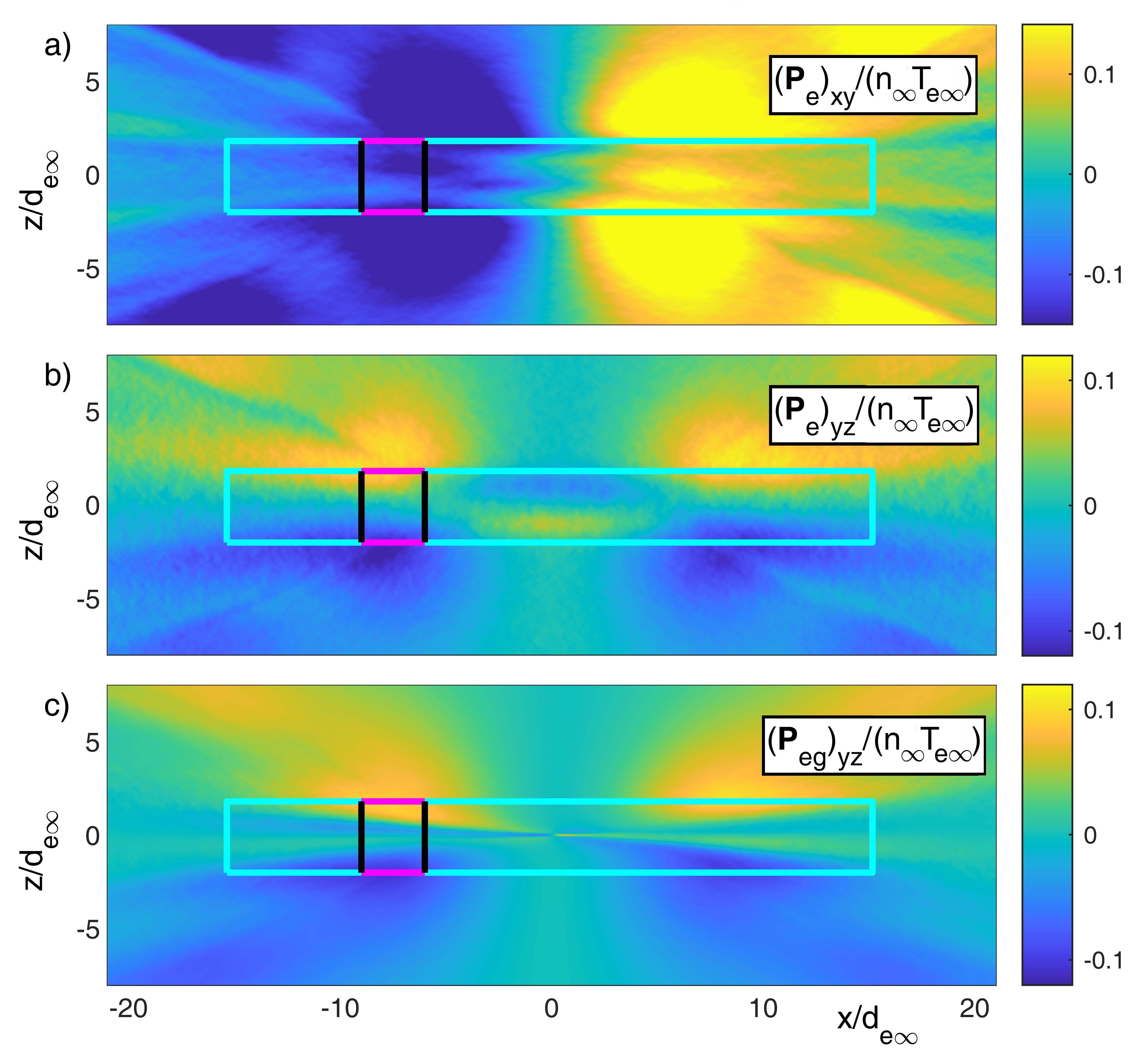
Figure 12: Considering the same simulation ($m_{i}/m_{e}=1836$ and $\beta_{e\infty}=2^{-4}$) as in Fig. 1, color contours are presented for a) ${p_{e}}_{xy}$, b) ${p_{e}}_{yz}$, and c) ${p_{eg}}_{yz}$. The EDR is outlined by the cyan rectangle, and a fluid-element is selected for analysis by the black/magenta square.

When away from the vicinity of the $X$-line, the $J\times B$-forces within the EDR are large (see Fig. 3(a)), and in Fig. 12 we explore how the large values of $({\bf J}\times{\bf B})_{y}$ are related to the electron pressure anisotropy that forms upstream of the EDR. For this, consider the small fluid element which in each panel is marked by the black/magenta square. Naturally, we can integrate Eq. (6) over the surface of this fluid element. For the RHS of Eq. (6) the largest contribution is from $\int(\nabla\cdot{\bf p}_{e})_{y}dA$. In turn, by the divergence theorem $\int(\nabla\cdot{\bf p}_{e})_{y}dA=\Delta{\bf p}_{exy}\,\Delta z+\Delta{\bf p}_{eyz}\,\Delta x$. Here, $\Delta{\bf p}_{exy}$ is the change in ${\bf p}_{exy}$ between the two black sides of the element, while $\Delta{\bf p}_{eyz}$ is the change in ${\bf p}_{eyz}$ between the two magenta sides. Comparing Figs. 12(a,b) it is clear that $|\Delta{\bf p}_{exy}|\ll|\Delta{\bf p}_{eyz}|$, such that $\int(\nabla\cdot{\bf p}_{e})_{y}dA\simeq\Delta{\bf p}_{eyz}\,\Delta x$.

We have now demonstrated that $\int({\bf J}\times{\bf B})_{y}dA\simeq\Delta{\bf p}_{eyz}\,\Delta x$. On the other hand, ${\bf J}\times{\bf B}=\nabla\cdot{\bf T}$, where ${\bf T}=(B^{2}/\mu_{0})({\bf bb}-{\bf I}/2)$ is the Maxwell stress tensor. By similar arguments to those applied when integrating $\int(\nabla\cdot{\bf p}_{e})_{y}dA$, we then find that $\int({\bf J}\times{\bf B})_{y}dA=\int(\nabla\cdot{\bf T})_{y}dA\simeq\Delta{\bf T}_{yz}\,\Delta x$. Note that for the fluid element with $\Delta x\simeq\Delta z$, we have $\Delta{\bf T}_{yz}\,\Delta x\gg\Delta{\bf T}_{xy}\,\Delta z$ due to the $\simeq 1/10$ aspect ratio of the full EDR. Neglecting $E_{y}$, the force balance constraint in Eq. (5) can then be expressed as $\Delta{\bf T}_{yz}\simeq\Delta{\bf p}_{eyz}$, and given these elements are asymmetric about $z=0$ this further reduces to ${\bf T}_{yz}\simeq{\bf p}_{eyz}$ along the upstream edge of the EDR. An identical analysis can be carried out for the forces in the $x$-direction, which yields the similar result that ${\bf T}_{xz}\simeq{\bf p}_{exz}$ along the upstream edge of the EDR.

The integrals over the fluid element involved the full pressure tensor ${\bf p}_{e}$, but by the divergence theorem the results only depend on the values of ${\bf p}_{e}$ at the upstream edge of the EDR; here ${\bf p}_{e}$ is well approximated by its CGL-form ${\bf p}_{e}\simeq{\bf p}_{eg}=({p_{e\parallel}}-p_{e\perp}){\bf bb}+p_{e\perp}{\bf I}$. To illustrate that ${\bf p}_{e}\simeq{\bf p}_{eg}$ outside the EDR, in Figs. 12(b,c) the profiles of ${\bf p}_{eyz}$ and ${\bf p}_{eg,yz}$ can be compared directly. Simple manipulations then show that the two force balance constraints that ${\bf T}_{yz}\simeq{\bf p}_{eyz}$ and ${\bf T}_{xz}\simeq{\bf p}_{exz}$, can now be expressed on a common form through the marginal firehose condition ${p_{e\parallel}}-p_{e\perp}=B^{2}/\mu_{0}$, again, applicable along the upstream edge of the EDR.

To summarize this analysis, we have shown that for the present simulation at $m_{i}/m_{e}=1836$ that $|en_{e}E_{y}|\ll|({\bf J}\times{\bf B})_{y}|\simeq|(\nabla\cdot{\bf p}_{e})_{y}|$. By integrating over a fluid element that spans the width of the EDR, it is then found that the strong ${\bf J}\times{\bf B}$-forces within the EDR are balanced by the force of the pressure anisotropy at the upstream edge of the EDR. In turn, at the upstream edge of the EDR the Lê-2009 equations of state Le et al. (2009) are applicable, and together with the force balance condition ${p_{e\parallel}}-p_{e\perp}=B^{2}/\mu_{0}$, this leads to the scaling law for the current across the EDR as expressed in Eq. (4). It is noteworthy here how the current across the EDR is expressed in terms of parameters evaluated far upstream of the reconnection region.

Appendix C: Connection to results of resistive-MHD

A critical reader may argue that the result in Eq. (15) was just obtained two different ways, and the statement in Eq. (16) therefore becomes trivial. However, here it should be noted that Eq. (15) was obtained based momentum balance constraints, while $\Delta p_{eyy,E}\simeq-enl_{u}E_{\mbox{\scriptsize rec}}$ applied to the RHS of Eq. (15) represents the separate issues related to electron heating. As such, Eq. (16) can be considered a meaningful mathematical expression describing the independence of $E_{\mbox{\scriptsize rec}}$ from the EDR dynamics, valid for any $E_{\mbox{\scriptsize rec}}$ sufficiently small that it does not alter the basic dynamics that lead to Eq. (15).

We also note that our interpretation of Eqs. (15) and (16) is not in conflict with results from resistive fluid models. For the particular case of an MHD plasma with resistivity $\eta$, the reconnection electric field is $E_{\mbox{\scriptsize rec}}=\eta J$, and the heating rate, ${\bf E}\cdot{\bf J}$, scales proportionally to $E_{\mbox{\scriptsize rec}}^{2}$. Power-balance arguments can then be invoked to quantify the much slower rate of reconnection characteristic of resistive MHD Manheimer and Lashmore-Davies (1984); Liu et al. (2022). In such fluid models with an imposed isotropic pressure, it is (by definition) not possible for $E_{\mbox{\scriptsize rec}}$ to change $p_{eyy}$ without introducing identical changes in $p_{exx}$ (and $p_{ezz}$). Therefore, Eq. (15) is then not applicable and the analysis applied in resistive MHD has no implications on the collisionless anti-parallel case studied here. In fact, as shown in Ref. Le, Egedal, and Daughton (2016), when the energy continuity equation is applied to the collisionless EDR of anti-parallel reconnection, we obtain a prediction of the net electron heating level across the EDR, which does not impose a constraint on $E_{\mbox{\scriptsize rec}}$.

For the related case of collisionless guide-field reconnection, the structure of the EDR is qualitatively different as it does not include the jets of meandering electrons Le et al. (2009). Further investigations are therefore needed to determine if the present framework can be generalized to scenarios including an out-of-plane guide magnetic field.

Appendix D: Characteristic length scales of the simulation domains

Table 1: Parameters describing the numerical simulation sizes in the $x$-direction. In the $z$-direction the domains all have half the size of the $x$-direction. For example, for $m_{i}/m_{e}=1836$ the domains are characterized by $L_{x}/d_{ep}\times L_{z}/d_{ep}=1000\times 500$.

Table I.A: $L_{x}/d_{ep}$, $L_{x}/d_{ip}$, # of $x$-cells
$m_{i}/m_{e}=100$		200	400	800	1836
$L_{x}/d_{ep}$	500	707	1000	1000	1000
$L_{x}/d_{ip}$	50	50	50	35.35	23.34
# of $x$-cells	3960	3960	5632	5632	5632
Table I.B: $L_{x}/d_{e\infty}$
$m_{i}/m_{e}=100$		200	400	800	1836
$\beta_{e\infty}=2^{-1}$	433	612	866	866	866
$2^{-2}$	387	548	775	775	775
$2^{-3}$	327	463	655	655	655
$2^{-4}$	261	369	522	522	522
$2^{-5}$	199	281	397	397	397
$2^{-6}$	146	207	293	293	293
$2^{-7}$	106	150	212	212	212
Table I.C: $L_{x}/d_{i\infty}$
$m_{i}/m_{e}=100$		200	400	800	1836
$\beta_{e\infty}=2^{-1}$	43.3	43.3	43.3	30.6	20.2
$2^{-2}$	38.7	38.7	38.7	27.4	18.1
$2^{-3}$	32.7	32.7	32.7	23.1	15.3
$2^{-4}$	26.1	26.1	26.1	18.5	12.2
$2^{-5}$	19.9	19.9	19.9	14.0	9.3
$2^{-6}$	14.6	14.6	14.6	10.4	6.8
$2^{-7}$	10.6	10.6	10.6	7.5	4.9

References

- Dungey (1953) J. Dungey, “Conditions for the occurence of electrical discharges in astrophysical systems,” Philosophical Magazine 44, 725 (1953).
- Masuda et al. (1994) S. Masuda, T. Kosugi, H. Hara, and Y. Ogawaray, “A loop top hard x-reay source i a compact solar-flare as evidence for magnetic reconnection,” Nature 371, 495–497 (1994).
- McPherron, Russell, and Aubry (1973) R. McPherron, C. Russell, and M. Aubry, “Satellite studies of magnetospheric substorms on august 15, 1968 .9. phenomenological model for substorms,” J. Geophys. Res. 78, 3131–3149 (1973).
- Parker (1957) E. N. Parker, “Sweet’s mechanism for merging magnetic fields in conducting fluids,” J. Geophys. Res. 62, 509 (1957).
- Birn et al. (2001) J. Birn, J. F. Drake, M. A. Shay, B. N. Rogers, R. E. Denton, M. Hesse, M. Kuznetsova, Z. W. Ma, A. Bhattacharjee, A. Otto, and P. L. Pritchett, “Geospace environmental modeling (GEM) magnetic reconnection challenge,” J. Geophys. Res. 106, 3715–3719 (2001).
- Ohia et al. (2012) O. Ohia, J. Egedal, V. S. Lukin, W. Daughton, and A. Le, “Demonstration of Anisotropic Fluid Closure Capturing the Kinetic Structure of Magnetic Reconnection,” Phys. Rev. Lett. 109 (2012), 10.1103/PhysRevLett.109.115004.
- Shay et al. (1999) M. A. Shay, J. F. Drake, B. N. Rogers, and R. E. Denton, “The scaling of collisionless, magnetic reconnection for large systems,” Geophy. Res. Lett. 26, 2163–2166 (1999).
- Zweibel and Yamada (2016) E. G. Zweibel and M. Yamada, “Perspectives on magnetic reconnection,” Proc. R. Soc. A 472 (2016), 10.1098/rspa.2016.0479.
- Silin, Büchner, and Vaivads (2005) I. Silin, J. Büchner, and A. Vaivads, “Anomalous resistivity due to nonlinear lower-hybrid drift waves,” Physics of Plasmas 12, 062902 (2005), https://doi.org/10.1063/1.1927096 .
- Che, Drake, and Swisdak (2011) H. Che, J. F. Drake, and M. Swisdak, “A current filamentation mechanism for breaking magnetic field lines during reconnection,” Nature 474, 184–187 (2011).
- Muñoz, Büchner, and Kilian (2017) P. A. Muñoz, J. Büchner, and P. Kilian, “Turbulent transport in 2d collisionless guide field reconnection,” Physics of Plasmas 24, 022104 (2017), https://doi.org/10.1063/1.4975086 .
- Egedal et al. (2018) J. Egedal, A. Le, W. Daughton, B. Wetherton, P. A. Cassak, J. L. Burch, B. Lavraud, J. Dorelli, D. J. Gershman, and L. A. Avanov, “Spacecraft Observations of Oblique Electron Beams Breaking the Frozen-In Law During Asymmetric Reconnection,” Phys. Rev. Lett. 120 (2018), 10.1103/PhysRevLett.120.055101.
- Egedal et al. (2019) J. Egedal, J. Ng, A. Le, W. Daughton, B. Wetherton, J. Dorelli, D. Gershman, and A. Rager, “Pressure tensor elements breaking the frozen-in law during reconnection in earth’s magnetotail,” Phys. Rev. Lett. 123, 225101 (2019).
- Greess et al. (2021) S. Greess, J. Egedal, A. Stanier, W. Daughton, J. Olson, A. Le, R. Myers, A. Millet-Ayala, M. Clark, J. Wallace, D. Endrizzi, and C. Forest, “Laboratory verification of electron-scale reconnection regions modulated by a three-dimensional instability,” J. Geophys. Res. 126 (2021), 10.1029/2021JA029316.
- Schroeder et al. (2022) J. M. Schroeder, J. Egedal, G. Cozzani, Y. V. Khotyaintsev, W. Daughton, R. E. Denton, and J. L. Burch, “2D Reconstruction of Magnetotail Electron Diffusion Region Measured by MMS,” Geophy. Res. Lett. 49, e2022GL100384 (2022), e2022GL100384 2022GL100384, https://agupubs.onlinelibrary.wiley.com/doi/pdf/10.1029/2022GL100384 .
- Torbert et al. (2018) R. B. Torbert, J. L. Burch, T. D. Phan, M. Hesse, M. R. Argall, J. Shuster, R. E. Ergun, L. Alm, R. Nakamura, K. J. Genestreti, D. J. Gershman, W. R. Paterson, D. L. Turner, I. Cohen, B. L. Giles, C. J. Pollock, S. Wang, L.-J. Chen, J. E. Stawarz, J. P. Eastwood, K. J. Hwang, C. Farrugia, I. Dors, H. Vaith, C. Mouikis, A. Ardakani, B. H. Mauk, S. A. Fuselier, C. T. Russell, R. J. Strangeway, T. E. Moore, J. F. Drake, M. A. Shay, Y. V. Khotyaintsev, P.-A. Lindqvist, W. Baumjohann, F. D. Wilder, N. Ahmadi, J. C. Dorelli, L. A. Avanov, M. Oka, D. N. Baker, J. F. Fennell, J. B. Blake, A. N. Jaynes, O. Le Contel, S. M. Petrinec, B. Lavraud, and Y. Saito, “Electron-scale dynamics of the diffusion region during symmetric magnetic reconnection in space,” Science (2018), 10.1126/science.aat2998, http://science.sciencemag.org/content/early/2018/11/14/science.aat2998.full.pdf .
- Ma et al. (2020) X. Ma, K. Nykyri, A. Dimmock, and C. Chu, “Statistical study of solar wind, magnetosheath, and magnetotail plasma and field properties: 12+ years of themis observations and mhd simulations,” Journal of Geophysical Research: Space Physics 125, e2020JA028209 (2020), e2020JA028209 10.1029/2020JA028209, https://agupubs.onlinelibrary.wiley.com/doi/pdf/10.1029/2020JA028209 .
- Le et al. (2013) A. Le, J. Egedal, O. Ohia, W. Daughton, H. Karimabadi, and V. S. Lukin, “Regimes of the Electron Diffusion Region in Magnetic Reconnection,” Phys. Rev. Lett. 110 (2013), 10.1103/PhysRevLett.110.135004.
- Egedal, Daughton, and Le (2012) J. Egedal, W. Daughton, and A. Le, “Large-scale electron acceleration by parallel electric fields during magnetic reconnection,” Nature Physics 8, 321–324 (2012).
- Egedal et al. (2015) J. Egedal, W. Daughton, A. Le, and A. L. Borg, “Double layer electric fields aiding the production of energetic flat-top distributions and superthermal electrons within magnetic reconnection exhausts,” Phys. Plasmas 22 (2015), 10.1063/1.4933055.
- Hesse et al. (1999) M. Hesse, K. Schindler, J. Birn, and M. Kuznetsova, “The diffusion region in collisionless magnetic reconnection,” Phys. Plasmas 6, 1781–1795 (1999), 40th Annual Meeting of the Division of Plasma Physics of the American-Physical-Society, New Orleans, Louisiana, Nov 16-20, 1998.
- Daughton, Scudder, and Homa (2006) W. Daughton, J. Scudder, and K. Homa, “Fully kinetic simulations of undriven magnetic reconnection with open boundary conditions,” Phys. Plasmas 13, 072101 (2006).
- Drake, Shay, and Swisdak (2008) J. F. Drake, M. A. Shay, and M. Swisdak, “The Hall fields and fast magnetic reconnection,” Phys. Plasmas 15 (2008), 10.1063/1.2901194.
- Shay, Drake, and Swisdak (2007) M. A. Shay, J. F. Drake, and M. Swisdak, “Two-scale structure of the electron dissipation region during collisionless magnetic reconnection,” Phys. Rev. Lett. 99 (2007), 10.1103/PhysRevLett.99.155002.
- Karimabadi, Daughton, and Scudder (2007) H. Karimabadi, W. Daughton, and J. Scudder, “Multi-scale structure of the electron diffusion region,” Geophy. Res. Lett. 34 (2007), 10.1029/2007GL030306.
- Kuznetsova, Hesse, and Winske (1998) M. M. Kuznetsova, M. Hesse, and D. Winske, “Kinetic quasi-viscous and bulk flow inertia effects in collisionless magnetotail reconnection,” J. Geophys. Res. 103, 199–213 (1998).
- Cassak, Liu, and Shay (2017) P. A. Cassak, Y. H. Liu, and M. A. Shay, “A review of the 0.1 reconnection rate problem,” Journal of Plasma Physics 83 (2017), 10.1017/S0022377817000666.
- Liu et al. (2017) Y.-H. Liu, M. Hesse, F. Guo, W. Daughton, H. Li, P. A. Cassak, and M. A. Shay, “Why does steady-state magnetic reconnection have a maximum local rate of order 0.1?” Phys. Rev. Lett. 118, 085101 (2017).
- Le et al. (2014) A. Le, J. Egedal, J. Ng, H. Karimabadi, J. Scudder, V. Roytershteyn, W. Daughton, and Y. H. Liu, “Current sheets and pressure anisotropy in the reconnection exhaust,” Phys. Plasmas 21 (2014), 10.1063/1.4861871.
- Stanier et al. (2015) A. Stanier, W. Daughton, L. Chacon, H. Karimabadi, J. Ng, Y. M. Huang, A. Hakim, and A. Bhattacharjee, “Role of ion kinetic physics in the interaction of magnetic flux ropes,” Phys. Rev. Lett. 115 (2015), 10.1103/PhysRevLett.115.175004.
- Le et al. (2010a) A. Le, J. Egedal, W. Daughton, J. F. Drake, W. Fox, and N. Katz, “Magnitude of the hall fields during magnetic reconnection,” Geophysical Research Letters 37 (2010a), https://doi.org/10.1029/2009GL041941, https://agupubs.onlinelibrary.wiley.com/doi/pdf/10.1029/2009GL041941 .
- Egedal, Le, and Daughton (2013) J. Egedal, A. Le, and W. Daughton, “A review of pressure anisotropy caused by electron trapping in collisionless plasma, and its implications for magnetic reconnection,” Phys. Plasmas 20 (2013), 10.1063/1.4811092.
- Montag, Egedal, and Daughton (2020) P. Montag, J. Egedal, and W. Daughton, “Influence of Inflow Density and Temperature Asymmetry on the Formation of Electron Jets during Magnetic Reconnection,” Geophy. Res. Lett. 47 (2020), 10.1029/2020GL087612.
- Le et al. (2009) A. Le, J. Egedal, W. Daughton, W. Fox, and N. Katz, “Equations of state for collisionless guide-field reconnection,” Phys. Rev. Lett. 102, 085001 (2009).
- Chew, Goldberger, and Low (1956) G. F. Chew, M. L. Goldberger, and F. E. Low, “The boltzmann equation and the one-fluid hydromagnetic equations in the absence of particle collisions,” Proc. Royal Soc. A 112, 236 (1956).
- Egedal et al. (2016) J. Egedal, B. Wetherton, W. Daughton, and A. Le, “Processes setting the structure of the electron distribution function within the exhausts of anti-parallel reconnection,” Phys. Plasmas 23 (2016), 10.1063/1.4972135.
- Egedal et al. (2009) J. Egedal, W. Daughton, J. F. Drake, N. Katz, and A. Le, “Formation of a localized acceleration potential during magnetic reconnection with a guide field,” Phys. Plasmas 16 (2009), 10.1063/1.3130732.
- Gurram, Egedal, and Daughton (2021) H. Gurram, J. Egedal, and W. Daughton, “Shear alfven waves driven by magnetic reconnection as an energy source for the aurora borealis,” Geophy. Res. Lett. 48 (2021), 10.1029/2021GL094201.
- Le et al. (2010b) A. Le, J. Egedal, W. Fox, N. Katz, A. Vrublevskis, W. Daughton, and J. F. Drake, “Equations of state in collisionless magnetic reconnection,” Phys. Plasmas 17, 055703 (2010b), 51st Annual Meeting of the Division of Plasma Physics of the American Physical Society, Atlanta, GA, NOV 02-06, 2009.
- Horiuchi and Sato (1997) R. Horiuchi and T. Sato, “Particle simulation study of collisionless driven reconnection in a sheared magnetic field,” Phys. Plasmas 4, 277–289 (1997).
- Shay and Drake (1998) M. Shay and J. Drake, “The role of electron dissipation on the rate of collisionless magnetic reconnection,” Geophy. Res. Lett. 25, 3759–3762 (1998).
- Roytershteyn et al. (2013) V. Roytershteyn, S. Dorfman, W. Daughton, H. Ji, M. Yamada, and H. Karimabadi, “Electromagnetic instability of thin reconnection layers: Comparison of three-dimensional simulations with MRX observations,” Physics of Plasmas (2013), 10.1063/1.4811371.
- Mandt, Denton, and Drake (1994) M. Mandt, R. Denton, and J. Drake, “Transition to whistler mediated magnetic reconnection,” Geophy. Res. Lett. 21, 73–76 (1994).
- Hesse, Zenitani, and Klimas (2008) M. Hesse, S. Zenitani, and A. Klimas, “The structure of the electron outflow jet in collisionless magnetic reconnection,” Phys. Plasmas 15 (2008), 10.1063/1.3006341.
- Le, Egedal, and Daughton (2016) A. Le, J. Egedal, and W. Daughton, “Two-stage bulk electron heating in the diffusion region of anti-parallel symmetric reconnection,” Phys. Plasmas 23 (2016), 10.1063/1.4964768.
- Bowers et al. (2009) K. Bowers, B. Albright, L. Yin, W. Daughton, V. Roytershteyn, B. Bergen, and T. Kwan, “Advances in petascale kinetic plasma simulation with VPIC and Roadrunner,” Journal of Physics: Conference Series 180, 012055 (10 pp.) (2009).
- Shay et al. (2004) M. Shay, J. Drake, M. Swisdak, and B. Rogers, “The scaling of embedded collisionless reconnection,” Phys. Plasmas 11, 2199–2213 (2004).
- Phan et al. (2018) T. D. Phan, J. P. Eastwood, M. A. Shay, J. F. Drake, B. U. O. Sonnerup, M. Fujimoto, P. A. Cassak, M. Oieroset, J. L. Burch, R. B. Torbert, A. C. Rager, J. C. Dorelli, D. J. Gershman, C. Pollock, P. S. Pyakurel, C. C. Haggerty, Y. Khotyaintsev, B. Lavraud, Y. Saito, M. Oka, R. E. Ergun, A. Retino, O. Le Contel, M. R. Argall, B. L. Giles, T. E. Moore, F. D. Wilder, R. J. Strangeway, C. T. Russell, P. A. Lindqvist, and W. Magnes, “Electron magnetic reconnection without ion coupling in earth’s turbulent magnetosheath,” Nature 557, 202+ (2018).
- Pyakurel et al. (2019) P. S. Pyakurel, M. A. Shay, T. D. Phan, W. H. Matthaeus, J. F. Drake, J. M. TenBarge, C. C. Haggerty, K. G. Klein, P. A. Cassak, T. N. Parashar, M. Swisdak, and A. Chasapis, “Transition from ion-coupled to electron-only reconnection: Basic physics and implications for plasma turbulence,” Phys. Plasmas 26 (2019), 10.1063/1.5090403.
- Olson et al. (2021) J. Olson, J. Egedal, M. Clark, D. A. Endrizzi, S. Greess, A. Millet-Ayala, R. Myers, E. E. Peterson, J. Wallace, and C. B. Forest, “Regulation of the normalized rate of driven magnetic reconnection through shocked flux pileup,” Journal of Plasma Physics 87 (2021), 10.1017/S0022377821000659.
- Greess et al. (2022) S. Greess, J. Egedal, A. Stanier, J. Olson, W. Daughton, A. Le, A. Millet-Ayala, C. Kuchta, and C. B. Forest, “Kinetic simulations verifying reconnection rates measured in the laboratory, spanning the ion-coupled to near electron-only regimes,” Phys. Plasmas 29 (2022), 10.1063/5.0101006.
- Vasyliunas (1975) V. M. Vasyliunas, “Theoretical models of magnetic-field line merging .1.” Reviews of Geophysics 13, 303–336 (1975).
- Cai, Ding, and Lee (1994) H. J. Cai, D. Q. Ding, and L. C. Lee, “Momentum transport near a magnetic x line in collisionless reconnection,” Journal of Geophysical Research: Space Physics 99, 35–42 (1994), https://agupubs.onlinelibrary.wiley.com/doi/pdf/10.1029/93JA02519 .
- Liu et al. (2022) Y.-H. Liu, P. Cassak, X. Li, M. Hesse, S.-C. Lin, and K. Genestreti, “First-principles theory of the rate of magnetic reconnection in magnetospheric and solar plasmas,” COMMUNICATIONS PHYSICS 5 (2022), 10.1038/s42005-022-00854-x.
- Payne et al. (2021) D. S. Payne, C. J. Farrugia, R. B. Torbert, K. Germaschewski, A. R. Rogers, and M. R. Argall, “Origin and structure of electromagnetic generator regions at the edge of the electron diffusion region,” Phys. Plasmas 28 (2021), 10.1063/5.0068317.
- Burch et al. (2020) J. L. Burch, J. M. Webster, M. Hesse, K. J. Genestreti, R. E. Denton, T. D. Phan, H. Hasegawa, P. A. Cassak, R. B. Torbert, B. L. Giles, D. J. Gershman, R. E. Ergun, C. T. Russell, R. J. Strangeway, O. Le Contel, K. R. Pritchard, A. T. Marshall, K. J. Hwang, K. Dokgo, S. A. Fuselier, L. J. Chen, S. Wang, M. Swisdak, J. F. Drake, M. R. Argall, K. J. Trattner, M. Yamada, and G. Paschmann, “Electron inflow velocities and reconnection rates at earth’s magnetopause and magnetosheath,” Geophy. Res. Lett. 47 (2020), 10.1029/2020GL089082.
- Ng et al. (2011) J. Ng, J. Egedal, A. Le, W. Daughton, and L. J. Chen, “Kinetic structure of the electron diffusion region in antiparallel magnetic reconnection,” Phys. Rev. Lett. 106 (2011), 10.1103/PhysRevLett.106.065002.
- Speiser (1965) T. Speiser, “Particle trajectories in model current sheets .i. analytical solutions,” J. Geophys. Res. 70, 4219 (1965).
- Shuster et al. (2015) J. R. Shuster, L. J. Chen, M. Hesse, M. R. Argall, W. Daughton, R. B. Torbert, and N. Bessho, “Spatiotemporal evolution of electron characteristics in the electron diffusion region of magnetic reconnection: Implications for acceleration and heating,” Geophy. Res. Lett. 42, 2586–2593 (2015).
- Divin et al. (2016) A. Divin, V. Semenov, D. Korovinskiy, S. Markidis, J. Deca, V. Olshevsky, and G. Lapenta, “A new model for the electron pressure nongyrotropy in the outer electron diffusion region,” Geophy. Res. Lett. 43, 10,565–10,573 (2016), https://agupubs.onlinelibrary.wiley.com/doi/pdf/10.1002/2016GL070763 .
- Le et al. (2015) A. Le, J. Egedal, W. Daughton, V. Roytershteyn, H. Karimabadi, and C. Forest, “Transition in electron physics of magnetic reconnection in weakly collisional plasma,” Journal of Plasma Physics 81 (2015), 10.1017/S0022377814000907.
- Rogers et al. (2001) B. N. Rogers, R. E. Denton, J. F. Drake, and M. A. Shay, “Role of dispersive waves in collisionless magnetic reconnection,” Phys. Rev. Lett. 8719, 195004 (2001).
- Cassak et al. (2015) P. A. Cassak, R. N. Baylor, R. L. Fermo, M. T. Beidler, M. A. Shay, M. Swisdak, J. F. Drake, and H. Karimabadi, “Fast magnetic reconnection due to anisotropic electron pressure,” PHYSICS OF PLASMAS 22 (2015), 10.1063/1.4908545.
- Manapat et al. (2006) M. Manapat, M. Øieroset, T. D. Phan, R. P. Lin, and M. Fujimoto, “Field-aligned electrons at the lobe/plasma sheet boundary in the mid-to-distant magnetotail and their association with reconnection,” Geophysical Research Letters 33 (2006), https://doi.org/10.1029/2005GL024971, https://agupubs.onlinelibrary.wiley.com/doi/pdf/10.1029/2005GL024971 .
- Le et al. (2017) A. Le, W. Daughton, L. J. Chen, and J. Egedal, “Enhanced electron mixing and heating in 3-D asymmetric reconnection at the Earth’s magnetopause,” Geophy. Res. Lett. 44, 2096–2104 (2017).
- Egedal et al. (2008) J. Egedal, W. Fox, N. Katz, M. Porkolab, M. Øieroset, R. P. Lin, W. Daughton, and D. J. F., “Evidence and theory for trapped electrons in guide field magnetotail reconnection,” J. Geophys. Res. 113, A12207 (2008).
- Manheimer and Lashmore-Davies (1984) W. M. Manheimer and C. Lashmore-Davies, “Mhd (magnetohydrodynamics) instabilities in simple plasma configuration,” (1984), https://www.osti.gov/biblio/6204270 .