Quadratic Programming for Continuous Control of Safety-Critical Multi-Agent Systems Under Uncertainty

Abstract

This paper studies the control problem for safety-critical multi-agent systems based on quadratic programming (QP). Each controlled agent is modeled as a cascade connection of an integrator and an uncertain nonlinear actuation system. In particular, the integrator represents the position-velocity relation, and the actuation system describes the dynamic response of the actual velocity to the velocity reference signal. The notion of input-to-output stability (IOS) is employed to characterize the essential velocity-tracking capability of the actuation system. The uncertain actuation dynamics may cause infeasibility or discontinuous solutions of QP algorithms for collision avoidance. Also, the interaction between the controlled integrator and the uncertain actuation dynamics may lead to significant robustness issues. By using nonlinear control methods and numerical optimization methods, this paper first contributes a new feasible-set reshaping technique and a refined QP algorithm for feasibility, robustness, and local Lipschitz continuity. Then, we present a nonlinear small-gain analysis to handle the inherent interaction for guaranteed safety of the closed-loop multi-agent system. The proposed methods are illustrated by numerical simulations and a physical experiment.

I Introduction

Attaining primary objectives while satisfying motion constraints is an essential yet challenging task for vehicles and robotic systems. This has been one of the most attractive topics in the interdisciplinary literature of controls and robotics in the past decades [1, 2, 3, 4, 5, 6].

Early utilized in constrained optimization [7], barrier functions have been employed to characterize state constraints for nonlinear control systems. Control barrier functions have been developed to enable constrained control designs [8, 9, 10, 11, 12, 13, 14, 15, 16]. The substantial relationship between control barrier functions and control Lyapunov functions [17] opens the door to a systematic development of a multi-objective control theory [18]. In particular, the recent advancement of control barrier functions relaxes the requirement of invariance of every level set (see [19] for zeroing barrier functions). Still, it only assumes an increasing property of the barrier function when the system state is outside the desired safety set. Moreover, for a control-affine nonlinear system, an appropriately defined control barrier function entails linear inequality constraints on admissible control inputs to keep the system state inside the desired set. See [20] for a discussion on the half-space robustness property of Sontag’s formula [21], and pointwise minimum norm formula [22]. This treatment allows computationally efficient integration of different control strategies to fulfill conflicting constraints.

Indeed, quadratic programming (QP) is a powerful tool for real-time synthesis of controllers by incorporating different specifications simultaneously [23, 24, 25]. For a system subject to motion constraints, a QP algorithm calculates the admissible control input that fulfills the constraints and is as close as possible to the set of control inputs for primary objectives [18]. The notions of robust barrier functions [18, 20] and input-to-state safety [26, 27] have been developed to handle perturbations. The study of Lipschitz continuity of QP-based control laws is not only of theoretical interest for well-defined solutions of closed-loop systems but also beneficial to avoiding chattering and other unexpected transient behaviors in practice [28, 29, 18, 20]. The integration of barrier functions and QP algorithms have found various applications, including automotive safety [18], robotic locomotion and manipulation [29, 30], multi-robot systems [31, 32, 33]. See [34] for a recent survey on control barrier functions and QP-based controller synthesis.

Other velocity obstacle approach [35, 36] calculates the set of feasible velocities for constrained motions. Still, the underlying assumption of piecewise continuous speed or acceleration possibly results in limited robustness to dynamic uncertainties. We also recognize the refined designs to address the discontinuity issue [37]. Interested readers may also consult the recent paper [38] for a comparative study of control barrier functions and the popular artificial potential fields [39].

This paper investigates the safety control problem for a class of mobile agents modeled as a cascade connection of an integrator and an uncertain actuation system. Such a system setup covers a broad class of practical control systems. If the dynamics of the actuation system are neglectable, then the proposed model is reduced to an integrator, which is known as an essential model for safety control. Some other systems, e.g., double-integrators and Euler-Lagrange systems, can also be transformed into our model by introducing appropriate virtual control laws. Interestingly, the identified model of a quadrotor is in the form of our model (see Section VI). Unsurprisingly, dynamic uncertainties challenge the robustness and computational feasibility of QP-based algorithms and may cause the collision avoidance performance to deteriorate (as illustrated in Figure 1).

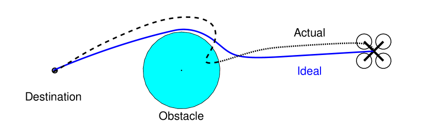
Figure 1: The ideal path is collision-free, while uncertain actuation dynamics may cause collision.

This paper assumes an essential velocity-tracking capability for the actuation system, which is described by the notion of input-to-output stability (IOS) [40, 41]. In the presence of uncertain actuation dynamics, a conventional QP algorithm may not be feasible, and the solution may be discontinuous even if it exists. Moreover, the uncertain actuation system leads to an unexpected feedback loop from the constrained position to the velocity-tracking error and possibly destroys the usual half-space robustness.

This paper proposes a seamless integration of numerical optimization and nonlinear control to address the major technical difficulty caused by uncertain actuation dynamics. Our first contribution lies in a new feasible-set reshaping technique by refining a standard QP algorithm for guaranteed feasibility, robustness, and local Lipschitz continuity. Based on the treatment above, the controlled multi-agent system is transformed into an interconnected system composed of two subsystems, one corresponding to the nominal controlled system subject to the velocity-tracking error and the other caused by the uncertain actuation dynamics. We employ gains to represent the interconnections and develop a nonlinear small-gain analysis to guarantee safety.

To the best of our knowledge, some techniques in this paper are reported for the first time. The feasible-set reshaping technique ensures (local) Lipschitz continuity of the solution of the refined QP algorithm and would be beneficial to other related problems with continuous motion constraints. The robustness analysis for collision avoidance subject to multiple safety constraints is still valuable when the controlled agents are free of uncertain actuation dynamics. The small-gain analysis takes advantage of the inherent interaction between the nominal system and the uncertain actuation dynamics. It motivates a new integration methodology for kinematics and dynamics control loops.

The rest of the paper is organized as follows. Section II introduces the system setup and gives the collision avoidance problem formulation. In Section III, we employ two examples to discuss the technical difficulty caused by the uncertain actuation dynamics. The main result of a refined QP algorithm with a reshaped feasible set is presented in Section IV. The proof of the main result, given in Section V, is based on several new properties of the refined QP algorithm and local small-gain analysis. In Section VI, we employ numerical simulations and a physical experiment based on quadrotors to illustrate the validity of the proposed method. Section VII presents some concluding remarks. Due to space limitations, some proofs are placed in the technical report [42].

Notations

The following notations are given to make the paper self-contained.

We use $|x|$ to represent the Euclidean norm of $x\in\mathbb{R}^{n}$, and use $|A|$ to represent the induced $2$-norm of $A\in\mathbb{R}^{m\times n}$. For a nonzero real vector $x$, we denote $\hat{x}=x/|x|$. For vectors $x,x^{\prime}\in\mathbb{R}^{n}$, $x<x^{\prime}$ represents that the corresponding elements $x_{i}$ and $x_{i}^{\prime}$ satisfy $x_{i}<x_{i}^{\prime}$. The notations $\leq$, $>$ and $\geq$ are defined in the same way for vectors. For a real vector $x$, $\min\{x\}$ and $\max\{x\}$ denote the smallest and the largest element of $x$, respectively. For a real vector $x$, $[x]_{i}$ represents the $i$-th element. For a real matrix $A$, $[A]_{i,j}$, $[A]_{i,:}$ and $[A]_{:,j}$ represent the element at the $i$-th row and the $j$-th column, the $i$-th row vector and the $j$-th column vector of the matrix $A$, respectively, $\min\{A\}$ denotes a column vector containing the minimum value of each row, and $\max\{A\}$ denotes a column vector containing the maximum value of each row. We use $\otimes$ to represent the Kronecker product, and use $\odot$ to represent the Hadamard product. In particular, for $A\in\mathbb{R}^{m\times n}$ and $B\in\mathbb{R}^{1\times n}$, $C=A\odot B$ is defined by $[C]_{i,j}=[A]_{i,j}[B]_{1,j}$. For $A\in\mathbb{R}^{n\times n}$, $\lambda_{\max}(A)$ and $\lambda_{\min}(A)$ take the maximum eigenvalue and the minimum eigenvalue, respectively, and $\sigma_{\max}(A)$ and $\sigma_{\min}(A)$ take the maximum singular value and the minimum singular value, respectively.

For a measurable and locally essentially bounded signal $u:\mathbb{R}_{+}\rightarrow\mathbb{R}^{m}$, $\|u\|_{[t_{1},t_{2})}=\operatorname{ess~{}sup}_{\tau\in[t_{1},t_{2})}|u(\tau)|$, and $\|u\|_{t}=\|u\|_{[0,t)}$. Let $f(t)$ be a real-valued function defined over an open interval $(a,b)$. The upper right Dini derivative of $f(t)$ at $t_{0}\in(a,b)$ is defined as $D^{+}f(t_{0})=\limsup_{t\rightarrow t_{0^{+}}}(f(t)-f(t_{0}))/(t-t_{0})$.

The definitions of positive definite functions and functions of classes $\mathcal{K}$, $\mathcal{K}_{\infty}$ and $\mathcal{KL}$ can be found in [43]. A continuous function $\alpha:(-a,b)\rightarrow(-c,\infty)$ with constants $a,b,c>0$ is said to be of class $\mathcal{K}^{e}$ if it is strictly increasing and $\alpha(0)=0$. A continuously differentiable function $\mu:(-a,\infty)\rightarrow(0,b)$ with constants $a$, $b>0$ is said to be of class $\mathcal{M^{-}C}$, denoted by $\mu\in\mathcal{M^{-}C}$, if it is strictly decreasing, strictly convex, $\lim_{s\rightarrow\infty}\mu(s)=0$, and $\lim_{s\rightarrow\infty}\partial\mu(s)/\partial s=0$. $\operatorname{Id}$ denotes the identity function. $\operatorname{sat}(r):=\max\{\min\{r,1\},0\}$ is a saturation function defined for $r\in\mathbb{R}$.

II Problem Formulation and Preliminaries

This section first introduces the class of systems to be studied in this paper, and then gives the problem formulation of collision avoidance.

Suppose there are $n_{a}$ agents and $n_{o}$ obstacles indexed by

$$\mathcal{N}_{a}=\{1,\ldots,n_{a}\},~{}~{}~{}\mathcal{N}_{o}=\{n_{a}+1,\ldots,n_{a}+n_{o}\},$$ (1)

respectively. Denote $\mathcal{N}_{ao}=\mathcal{N}_{a}\cup\mathcal{N}_{o}$, and $n_{ao}=n_{a}+n_{o}$. For each $i\in\mathcal{N}_{ao}$, we use $p_{i}\in\mathbb{R}^{n}$ to represent the position of the mobile agent or the obstacle, and use

$$p=\left[p_{1},\ldots,p_{n_{ao}}\right]$$ (2)

to represent the positions of all the mobile agents and the obstacles.

For $i\in\mathcal{N}_{a}$, each agent $i$ is modeled as a cascade connection of a nominal system and an uncertain actuation system. Specifically, the nominal system is represented by

$$\dot{p}_{i}=v_{i},$$ (3)

where $v_{i}\in\mathbb{R}^{n}$ is the velocity. The velocity $v_{i}$ is generated by an actuation system, which is in the general form:

$$\dot{z}_{i}=f(z_{i},v^{*}_{i}),~{}~{}v_{i}=g(z_{i},v^{*}_{i})$$ (4)

where $z_{i}\in\mathbb{R}^{m}$ is the state of the actuation system, $v^{*}_{i}\in\mathbb{R}^{n}$ represents the velocity reference signal, and $f$ and $g$ are locally Lipschitz functions.

The multi-agent system with each agent described by (3)-(4) is said to be safe if under some specific initial conditions

$$\min_{i\in\mathcal{N}_{a},~{}j\in\mathcal{N}_{ao}\setminus\{i\}}|p_{i}(0)-p_{j}(0)|\geq\underline{D}_{0},~{}~{}\max_{i\in\mathcal{N}_{a}}|z_{i}|\leq\bar{z}_{0},$$ (5)

with $\underline{D}_{0}$, $\bar{z}_{0}>0$, the relative positions of the multi-agent system satisfy

$$\min_{i\in\mathcal{N}_{a},~{}j\in\mathcal{N}_{ao}\setminus\{i\}}|p_{i}(t)-p_{j}(t)|\geq D,$$ (6)

for all $t\geq 0$, where $D>0$ is the safety distance.

We use $v_{i}^{c}\in\mathbb{R}^{n}$ to represent the velocity command signal for primary control objective. The safety control problem is concerned about designing controllers for the agents to incorporate the velocity command signals and the safety qualifications. The expected control system is shown in Figure 2.

Figure 2: Block diagram of the safety control system.

II-A Assumptions on the Actuation Systems and the Velocity Command Signals

In the presence of the uncertain actuation dynamics, the actual velocity $v_{i}$ may not equal to the velocity reference signal $v^{*}_{i}$. Define velocity-tracking error

$$\tilde{v}_{i}=v_{i}-v^{*}_{i}.$$ (7)

Then, the nominal system (3) can be rewritten as

$$\dot{p}_{i} =v_{i}=v^{*}_{i}+\tilde{v}_{i}.$$ (8)

In practice, it is essential that the actuation system is inherently stable and admits some velocity-tracking capability. In this paper, we assume that for a constant reference signal $v^{*}_{i}$, the actual velocity $v_{i}$ asymptotically converges to $v^{*}_{i}$, and for a time-varying $v^{*}_{i}$, the tracking error $\tilde{v}_{i}$ depends on the changing rate of $v^{*}_{i}$.

Suppose that the velocity reference signal $v^{*}_{i}$ is locally Lipschitz on the time-line, and denote

$$v^{*d}_{i}(t)=D^{+}v^{*}_{i}(t).$$ (9)

The following assumption is made on the uncertain actuation system.

Assumption 1 (Stability and reference-tracking capability of the actuation system)

Consider the actuation system (4). There exist locally Lipschitz functions $\alpha_{z1},\alpha_{z2},\gamma^{v^{*d}}_{\tilde{v}}\in\mathcal{K}$ and constants $c_{\tilde{v}}\geq 1$ and $\lambda>0$ such that for any $z_{i}(0)$ and any locally Lipschitz and bounded $v_{i}^{*}$,

$$|\tilde{v}_{i}(t)| \leq\beta_{\tilde{v}}(|z_{i}(0)|,t)+\gamma^{v^{*d}}_{\tilde{v}}(\|v^{*d}_{i}\|_{t})$$ (10)

$$|z_{i}(t)| \leq\alpha_{z1}(|z_{i}(0)|)+\alpha_{z2}(\|v^{*}_{i}\|_{t})$$ (11)

hold for all $t\geq 0$, where $\beta_{\tilde{v}}(s,t)=c_{\tilde{v}}e^{-\lambda t}s$ for $s,t\in\mathbb{R}_{+}$.

Remark 1

With the velocity-reference signal $v^{*}_{i}$’s Dini derivative as the input and the velocity-tracking error $\tilde{v}_{i}$ as the output, property (10) employs the notion of IOS to characterize the velocity-tracking capability: $\tilde{v}_{i}$ ultimately converges to the range of $\gamma^{v^{*d}}_{\tilde{v}}(\|v^{*d}\|_{\infty})$. Given bounded velocity reference signal $v^{*}_{i}$, property (11) guarantees the boundedness of state $z_{i}$. See, e.g., [41, 44, 45] for tutorials of the related notions.

Remark 2

Suppose the dynamics of the actuation system is neglectable. In that case, i.e., $v^{*}_{i}\equiv v_{i}$, the agent model is reduced to a single-integrator, which has been widely studied in the literature of safety control [46]. The double-integrator model [31] can also be transformed into the form of (3)-(4) by introducing a virtual control law to the velocity loop. Interestingly, the experimental data of a quadrotor in Section VI also coincides with model (3)-(4) and satisfies Assumption 1.

Example 1 gives a condition for linear control systems to satisfy Assumption 1.

Example 1 (Reference tracking capability of linear control systems)

Consider a linear control system

$$\dot{z}=Az+Bv^{*},~{}~{}v=Cz$$ (12)

where $z\in\mathbb{R}^{m}$ is the state, $v\in\mathbb{R}^{n}$ is the output, $v^{*}\in\mathbb{R}^{n}$ is the input, and $A$, $B$ and $C$ are real matrices with appropriate dimensions. It is assumed that $A$ is a Hurwitz matrix and satisfies

$$CA^{-1}B=-I_{n\times n}.$$ (13)

Define the tracking error $\tilde{v}=v-v^{*}$. For any constant input $v^{*}$, condition (13) implies that $\lim_{t\rightarrow\infty}\tilde{v}(t)=0$.

Suppose that $v^{*}$ is continuously differentiable, and denote $v^{*d}(t)=\dot{v}^{*}(t)$. Then, define $\zeta=Az+Bv^{*}$. Direct calculation yields:

$$\dot{\zeta} =A\dot{z}+Bv^{*d}=A\zeta+Bv^{*d},$$ (14)

$$\tilde{v} =Cz-v^{*}=CA^{-1}(\zeta-Bv^{*})-v^{*}=CA^{-1}\zeta.$$ (15)

Because $A$ is Hurwitz, the transformed linear control system (14)–(15) is stable. Property (10) can be proved by directly applying the definition of IOS-Lyapunov function [47]; see Section VI-A for details. $\Diamond$

In practice, $v^{c}_{i}$ is generated by the primary controller. Without loss of generality, we make the following assumption on the velocity command signal $v_{i}^{c}$.

Assumption 2 (Boundedness of the velocity command and its derivative)

For each $i\in\mathcal{N}_{a}$, $v_{i}^{c}$ is continuously differentiable with respect to time, and there exist positive constants $\bar{v}^{c}$ and $\bar{v}^{cd}$ such that

$$|v^{c}_{i}(t)|\leq\bar{v}^{c},~{}~{}|\dot{v}^{c}_{i}(t)|\leq\bar{v}^{cd}$$ (16)

for all $t\geq 0$.

II-B Characterization of Safety

For the multi-agent system (3)–(4), define

$$\tilde{p}_{ij}=p_{i}-p_{j}$$ (17)

to represent the relative positions. Then, from (8), we have

$$\dot{\tilde{p}}_{ij}=v_{i}-v_{j}=v^{*}_{i}-v^{*}_{j}+\tilde{v}_{i}-\tilde{v}_{j}.$$ (18)

To describe the safety of agent $i$ with respect to another agent or an obstacle $j$, we define

$$V(\tilde{p}_{ij})=\mu(|\tilde{p}_{ij}|-D_{s}),$$ (19)

where $\mu:(-D_{s},\infty)\rightarrow\mathbb{R}_{+}$ is an $\mathcal{M^{-}C}$ function and $D_{s}\in\mathbb{R}_{+}$ is safety margin. If the velocity reference signals $v^{*}_{i}$ and $v^{*}_{j}$ satisfy

$$-\hat{\tilde{p}}_{ij}^{T}(v^{*}_{i}-v^{*}_{j})\leq-\alpha_{V}(V(\tilde{p}_{ij})-\mu(0))$$ (20)

with $\alpha_{V}\in\mathcal{K}^{e}$, then along the trajectories of (18), we have

$$\nabla V\dot{\tilde{p}}_{ij}\leq\frac{\partial\mu(|\tilde{p}_{ij}|-D_{s})}{\partial(|\tilde{p}_{ij}|-D_{s})}\left(\alpha_{V}(V(\tilde{p}_{ij})-\mu(0))+\hat{\tilde{p}}_{ij}^{T}(\tilde{v}_{i}-\tilde{v}_{j})\right),$$ (21)

and thus

$$V(\tilde{p}_{ij})\geq\left(\alpha_{V}^{-1}(|\tilde{v}_{i}|+|\tilde{v}_{j}|)+\mu(0)\right)\Rightarrow\nabla V\dot{\tilde{p}}_{ij}\leq 0.$$ (22)

If the initial states satisfy $V(\tilde{p}_{ij}(0))\leq\mu(D-D_{s})$, and the velocity-tracking errors satisfy $\|\tilde{v}_{i}\|_{\infty}+\|\tilde{v}_{j}\|_{\infty}\leq\alpha_{V}(\mu(D-D_{s})-\mu(0))$, then

$$V(\tilde{p}_{ij}(t))\leq\mu(D-D_{s})$$ (23)

holds for all $t\geq 0$, which means safety by recalling equation (6).

Remark 3

If the agents are free of uncertain actuation dynamics, then the safety control problem would be readily solvable by applying barrier-function-based QP designs[16] and using the idea of forward invariance [18, Theorem 1]. However, for the class of multi-agent systems with uncertain actuation dynamics, the velocity-tracking errors may violate the safety constraint; see the discussions in Section III.

III Limitations of Standard Designs

This section employs examples to discuss the technical difficulty caused by the uncertain actuation dynamics. It is shown that the velocity-tracking errors may either lead to infeasibility of conventional QP-based controllers, or result in non-Lipschitz solutions. A non-Lipschitz solution may cause unexpected transient response of the uncertain actuation system and destroy the safety of the controlled agent.

III-A A QP-based Controller with an Extended Safety Margin

For convenience of notations, denote

$$V_{ij}(t) =V(\tilde{p}_{ij}(t)).$$ (24)

Given the velocity command $v^{c}_{i}$ for the primary control objective, inspired by the QP-based control strategy [31, 27], one may choose the actual velocity reference signal $v_{i}^{*}$ such that safety is ensured and at the same time $v_{i}^{*}$ is as close to the velocity command $v_{i}^{c}$ as possible:

$$v^{*}_{i} =\operatornamewithlimits{argmin}_{v^{*}_{i}\in\mathcal{P}^{o}_{i}(p)}\frac{1}{2}v^{*T}_{i}v^{*}_{i}-v^{cT}_{i}v^{*}_{i}$$ (25)

where

$$\mathcal{P}_{i}^{o}(p)=\left\{v^{*}_{i}\in\mathbb{R}^{n}:A^{o}_{i}(p)v^{*}_{i}+a^{o}_{i}(p)\leq 0\right\}$$ (26)

is the feasible set with

$$A^{o}_{i}(p) =[-\hat{\tilde{p}}_{i1},\ldots,-\hat{\tilde{p}}_{i(i-1)},-\hat{\tilde{p}}_{i(i+1)},\ldots,-\hat{\tilde{p}}_{in_{ao}}]^{T},$$ (27)

$$a^{o}_{i}(p) =[\alpha_{V}(V_{i1}-\mu_{0}),\ldots,\alpha_{V}(V_{i(i-1)}-\mu_{0}),\ldots$$

$$~{}~{}~{}~{}~{}~{}\alpha_{V}(V_{i(i+1)}-\mu_{0}),\ldots,\alpha_{V}(V_{in_{ao}}-\mu_{0})]^{T}.$$ (28)

Here, $\alpha_{V}$ is a continuously differentiable class $\mathcal{K}^{e}$ function, and $\mu_{0}=\mu(0)$. To avoid singularity, the algorithm requires $\tilde{p}_{ij}\neq 0$ for $i\in\mathcal{N}_{a}$ and $j\in\mathcal{N}_{ao}\setminus\{i\}$.

However, the velocity-tracking errors $\tilde{v}_{i}$ may violate the safety constraint of the conventional QP-based design [18, 20]. An intuitive solution is to extend the safety margin [48], which, however, still may not guarantee the feasibility of the QP algorithm if the total number of the constraints is larger than one; see Example 2.

Example 2 (Possible infeasibility of a conventional QP algorithm by extending safety margin to handle velocity-tracking error)

Consider the scenario involving one mobile agent with position $p_{1}$ and two obstacles with positions $p_{2}$ and $p_{3}$; see Figure 3. In this example, we consider $p_{2}=[0.5;0.5]$, $p_{3}=-[0.5;0.5]$, and $v_{1}^{c}=[1;-1]$. If the velocity-tracking error is neglectable, then one may consider

$$v_{1}^{*}=\operatornamewithlimits{argmin}_{v_{1}^{*}\in\mathcal{P}_{1}^{o}}\frac{1}{2}v^{*T}_{1}v^{*}_{1}-v^{cT}_{1}v^{*}_{1}$$ (29)

where $\mathcal{P}_{1}^{o}=\{v_{1}^{*}\in\mathbb{R}^{n}:A_{1}^{o}v_{1}^{*}+a_{1}^{o}\leq 0\}$ with $A_{1}^{o}=[-\hat{\tilde{p}}_{12},-\hat{\tilde{p}}_{13}]^{T}$ and $a_{1}^{o}=[|\tilde{p}_{12}|^{-1}-D^{-1},|\tilde{p}_{13}|^{-1}-D^{-1}]^{T}$.

When the velocity-tracking error is nonzero, one may consider extending the safety margin and redesigning the safety controller with new $a_{1}^{o}=[|\tilde{p}_{12}|^{-1}-D^{-1}_{s};|\tilde{p}_{13}|^{-1}-D^{-1}_{s}]$. But, such a treatment may result in an empty feasible set in specific cases. For example, in the case of $D=0.6$ and $D_{s}=1$, when $p_{1}=[0;0]$, the feasible set $\mathcal{P}_{1}^{o}$ in (26) should satisfy $\sqrt{2}^{-1}[1,1;-1,-1]v^{*}\leq(\sqrt{2}-1)[1;1]$, and thus is empty. $\Diamond$

Figure 3: Infeasibility of the QP algorithm by extending the safety margin to handle the velocity-tracking error.

III-B Introducing a Relaxation Parameter

An alternative solution is to introduce a relaxation parameter [18, 31, 20] to the QP algorithm as

$$\left[\begin{array}[]{@{}c@{}}v^{*}_{i}\\ \delta_{i}\end{array}\right]=\operatornamewithlimits{argmin}_{[v_{i}^{*};\delta_{i}]\in\mathcal{P}_{i}^{s}(p)}\frac{1}{2}\left[\begin{array}[]{@{}c@{}}v^{*}_{i}\\ \delta_{i}\end{array}\right]^{T}\left[\begin{array}[]{@{}c@{}}v^{*}_{i}\\ \delta_{i}\end{array}\right]-\left[\begin{array}[]{@{}c@{}}v_{i}^{c}\\ \delta\end{array}\right]^{T}\left[\begin{array}[]{@{}c@{}}v^{*}_{i}\\ \delta_{i}\end{array}\right]$$ (40)

where $\delta_{i}$ is the relaxation parameter, $\delta$ is intended to compensate the effect of $\delta_{i}$,

$$\mathcal{P}_{i}^{s}(p)=\left\{[v_{i}^{*};\delta_{i}]:A_{i}^{s}(p)v_{i}^{*}+a_{i}^{s}(p)\delta_{i}\leq 0,\delta_{i}\in[0,\delta]\right\}$$ (41)

is the feasible set with $A_{i}^{s}(p)=A^{o}_{i}(p)$ defined in (27), and without loss of generality,

$$a_{i}^{s}(p) =\frac{1}{\delta}a_{i}^{o}(p)$$ (42)

where $a_{i}^{o}(p)$ is defined in (28).

Clearly, if $\tilde{p}_{ij}\neq 0$ for $i\in\mathcal{N}_{a}$ and $j\in\mathcal{N}_{ao}\setminus\{i\}$, then zero is always an element of $\mathcal{P}_{i}^{s}(p)$ and thus the QP algorithm is always feasible. However, such a modification does not guarantee the Lipschitz continuity of the solution; see Example 3.

Example 3 (Lipschitz continuity of the solution to a conventional QP algorithm not guaranteed by simply adding a relaxation parameter)

Still consider the case in Example 2. We use $(\breve{A}_{i}^{s},\breve{a}_{i}^{s})$ to represent the non-redundant active constraints of the QP algorithm defined by (40), with $\breve{A}_{i}^{s}$ and $\breve{a}_{i}^{s}$ being submatrices of $A_{i}^{s}$ and $a_{i}^{s}$, respectively. From [49, Example 2.1.5], the solution to the QP algorithm is

$$v_{1}^{*}=v^{c}_{1}-\breve{A}_{1}^{sT}(\breve{A}_{1}^{s}\breve{A}_{1}^{sT}+\breve{a}_{1}^{s}\breve{a}_{1}^{sT})^{-1}(\breve{A}_{1}^{s}v_{1}^{c}+\breve{a}_{1}^{s}\delta).$$ (43)

Suppose that the non-redundant active constraints are not changed in some domain of $p$. Then, in this domain, taking the partial derivative of $v_{1}^{*}$ with respect to $\breve{a}_{1}^{s}$ yields

$$\frac{\partial v_{1}^{*}}{\partial\breve{a}_{1}^{sT}}= \frac{\delta\Lambda_{2}(2\Lambda_{3}\Lambda_{0}^{-1}-\Lambda_{1})-2\Lambda_{2}\Lambda_{3}\Lambda_{2}^{T}v_{1}^{c}\breve{a}_{1}^{sT}\Lambda_{0}^{-1}}{\Lambda_{1}^{2}}+$$

$$\frac{(v_{1}^{cT}\Lambda_{2}\breve{a}^{s}_{1})\otimes\Lambda_{2}+(v_{1}^{cT}\Lambda_{2})\otimes(\Lambda_{2}\breve{a}_{1}^{s})}{\Lambda_{1}}$$ (44)

where $\Lambda_{0}=\breve{A}_{1}^{s}\breve{A}_{1}^{sT}$, $\Lambda_{1}=(1+\breve{a}^{sT}_{1}\Lambda_{0}^{-1}\breve{a}^{s}_{1})$, $\Lambda_{2}=\breve{A}^{sT}_{1}\Lambda_{0}^{-1}$ and $\Lambda_{3}=\breve{a}^{s}_{1}\breve{a}^{sT}_{1}$. $\breve{A}^{s}_{1}$ is consisted of the relative positions between the agent and the obstacles. Thus, $\sigma_{\min}(\breve{A}^{s}_{1})$ cannot be guaranteed to be lower bounded by a positive constant. This means that the solution to the QP algorithm may not be Lipschitz. Indeed, [50, Theorem 3.1] requires a positive lower bound of $\sigma_{\min}(\breve{A}^{s}_{1})$ to guarantee the Lipschitz continuity of the QP problem. In this numerical example, we consider $D=0.6$, $D_{s}=0.68$, $v^{c}_{1}=[1;-1]$, $p_{1}\in\{p:|p-p_{2}|\geq D,|p-p_{3}|\geq D~{}\}$, $p_{2}=[0.5;0.5]$, $p_{3}=-[0.5;0.5]$, $\delta=100$, $A^{s}_{1}(p)=[-\hat{\tilde{p}}_{12},-\hat{\tilde{p}}_{13}]^{T}$ and $a^{s}_{1}(p)=\delta^{-1}\left[|\tilde{p}_{12}|^{-1}-D^{-1}_{s},|\tilde{p}_{12}|^{-1}-D^{-1}_{s}\right]^{T}$. Figure 4 shows how $p_{1}$ influences $|v_{1}^{*}|$. One may observe the sudden change of $|v_{1}^{*}|$ when $p_{1}$ is close to zero. $\Diamond$

Figure 4: $|v_{1}^{*}|$ with respect to different $p_{1}$: Lipschitz continuity of the solution to the QP algorithm cannot be guaranteed by simply adding a relaxation parameter.

Examples 2 and 3 show that the methods mentioned above do not guarantee the local Lipschitz property of the solution to the QP algorithm with respect to time. However, the local Lipschitz continuity of the solution is viewed to be essential for the robustness of a QP algorithm in practical systems. In the system setup in this paper, the non-Lipschitz velocity reference signal may lead to a large gain from the barrier function to the velocity-tracking error and result in the unexpected dynamic response of the actuation system, which may violate the safety of the nominal system. This is also verified by the numerical example in Subsection VI-B.

IV New QP-based Design with Relaxation Parameter and Reshaped Feasible Region

In this section, we present our solution to the safety control problem involving multiple controlled mobile agents and multiple stationary obstacles. Our major contribution lies in a new class of QP-based controllers with relaxation parameters and reshaped feasible sets to address the non-Lipschitz issue discussed in Section III. To be specific, positive bases are used to reshape the feasible sets for ensured feasibility and Lipschitz continuity.

The proposed safety controller is in the form of

$$\left[\begin{array}[]{@{}c@{}}v^{*}_{i}\\ \delta_{i}\end{array}\right]=\operatornamewithlimits{argmin}_{[v_{i}^{*};\delta_{i}]\in\mathcal{P}_{i}^{r}(p)}\frac{1}{2}\left[\begin{array}[]{@{}c@{}}v^{*}_{i}\\ \delta_{i}\end{array}\right]^{T}\left[\begin{array}[]{@{}c@{}}v^{*}_{i}\\ \delta_{i}\end{array}\right]-\left[\begin{array}[]{@{}c@{}}v_{i}^{c}\\ \delta\end{array}\right]^{T}\left[\begin{array}[]{@{}c@{}}v^{*}_{i}\\ \delta_{i}\end{array}\right]$$ (55)

where

$$\mathcal{P}^{r}_{i}(p)=\left\{[v^{*}_{i};\delta_{i}]:~{}A^{r}_{i}v^{*}_{i}+a^{r}_{i}(p)\delta_{i}\leq 0,\delta_{i}\in[0,\delta]\right\}$$ (56)

is the reshaped feasible set. Here, $A^{r}_{i}\in\mathbb{R}^{n_{p}\times n}$ is a constant matrix with $n_{p}>n$, and satisfies that each row is a unit vector, any $n$ rows are linearly independent, and for any unit vector $\hat{u}\in\mathbb{R}^{n}$,

$$\min_{q\in\mathcal{Q}(\hat{u})}\max_{j\in\mathcal{J}(\hat{u})}[A^{r}_{i}]_{j,:}q >0,$$ (57)

$$\operatorname{card}(\mathcal{J}(\hat{u})) \geq n,$$ (58)

where $\mathcal{Q}(\hat{u})=\{q\in\mathbb{R}^{n}:q^{T}\hat{u}>0\}$, $\mathcal{J}(\hat{u})=\{j=1,\ldots,n_{p}:[A^{r}_{i}]_{j,:}\hat{u}\geq c_{A}\}$ with $c_{A}$ being a positive constant less than $1$, and $\operatorname{card}$ takes the cardinality.

We choose $a^{r}_{i}:\mathbb{R}^{n\times n_{ao}}\rightarrow\mathbb{R}^{n_{p}}$ as

$$a^{r}_{i}(p) =\max\left\{\varphi\left(A^{s}_{i}(p),a^{s}_{i}(p),\frac{c_{P}}{\delta}\right)\right\}$$ (59)

with

$$\varphi\left(A^{s}_{i},a_{i}^{s},\frac{c_{P}}{\delta}\right)=A^{r}_{i}A^{sT}_{i}\odot a_{i}^{sT}$$

$$~{}~{}~{}-\operatorname{sat}(c_{K}(c_{A}-A^{r}_{i}A^{sT}_{i}))\odot(A^{r}_{i}A^{sT}_{i}\odot a_{i}^{sT}+\frac{c_{P}}{\delta}),$$ (60)

where $c_{A}$ is associated with $A^{r}_{i}$ given in the definition of $\mathcal{J}(\hat{u})$, $c_{K}\geq c_{A}^{-1}$ and $c_{P}$ can be any positive constants, and $\delta$, $A^{s}_{i}$ and $a^{s}_{i}$ are defined in (40)–(41).

Condition (57) guarantees that any vector in $\mathbb{R}^{n}$ can be represented by a strictly positive combination of some row vectors of $A^{r}_{i}$ [51, Theorem 3.3]. Based on [50, Theorem 3.1], it can be proved that such an $A^{r}_{i}$ can be used to guarantee Lipschitz continuity of the solution to the QP algorithm. The existence of such an $A^{r}_{i}$ is proved in Subsection V-A as part of the proof of the main result in Theorem 1.

In Example 4, we examine the refined QP algorithm (55) in the same scenario as in Examples 2 and 3.

Example 4 (Lipschitz continuity of the solution to the QP algorithm guaranteed by adding a relaxation parameter and reshaping the feasible set)

Continue Example 3. We construct a $\mathcal{P}^{r}_{i}$ in the form of (56) and examine the solution to the QP algorithm (55) with a reshaped feasible set. For any specific odd integer $n_{p}\geq 5$, a typical $A^{r}_{i}\in\mathbb{R}^{n_{p}\times 2}$ consists of the outward normal vectors to an odd-sided regular polygon, that is, each row of $A^{r}_{i}$ is $[\cos(2\pi j/n_{p}),~{}\sin(2\pi j/n_{p})]$ for $j=1,\ldots,n_{p}$. Accordingly, $c_{A}=\cos(2\pi/n_{p})$. In the numerical simulation, we choose $n_{p}=5$, $c_{K}=1$, $c_{P}=5/2$ and $c_{A}=\cos(2\pi/5)$. Figure 5 shows the original and the reshaped feasible sets when $p_{1}=[-0.4;0.4]$. Figure 6 shows how $p_{1}$ influences $|v_{1}^{*}|$, which is in accordance with our expectation of Lipschitz continuity. $\Diamond$

Figure 5: The relaxed and the reshaped feasible sets with $S_{i}:~{}[A^{s}_{1}]_{i,:}v^{*}_{1}=-[a^{s}_{1}]_{i}\delta_{1}$ for $i=1,2$ and $R_{i}:~{}[A^{r}_{1}]_{i,:}v^{*}_{1}=-[a^{r}_{1}]_{i}\delta_{1}$ for $i=1,\ldots,5$. $R_{3}$ corresponds to a redundant constraint, and is outside the range of the figure.

Figure 6: $|v_{1}^{*}|$ with respect to different $p_{1}$: In the scenario of Example 3, the Lipschitz continuity of the solution to the QP algorithm can be guaranteed by adding a relaxation parameter and reshaping the feasible set.

When the relaxation parameter $\delta_{i}$ goes to zero, the robustness with respect to the velocity-tracking error $\tilde{v}_{i}$ is weakened (see equation (117) in the proof of Proposition 4). In this case, motivated by [31], we set $v_{i}^{*}=0$. Hence, the implemented safety controller is defined as

$$\left[\begin{array}[]{@{}c@{}}v^{*}_{i}(t)\\ \delta_{i}(t)\end{array}\right]\!=\!\begin{cases}\operatornamewithlimits{argmin}\limits_{[v^{*}_{i};\delta_{i}]\in\mathcal{P}^{r}_{i}(p)}\dfrac{1}{2}\left[\begin{array}[]{@{}c@{}}v^{*}_{i}\\ \delta_{i}\end{array}\right]^{T}\!\left[\begin{array}[]{@{}c@{}}v^{*}_{i}\\ \delta_{i}\end{array}\right]\!-\!\left[\begin{array}[]{@{}c@{}}v_{i}^{c}\\ \delta\end{array}\right]^{T}\!\left[\begin{array}[]{@{}c@{}}v^{*}_{i}\\ \delta_{i}\end{array}\right],\\ ~{}~{}~{}~{}~{}~{}~{}~{}~{}~{}~{}~{}~{}~{}~{}~{}~{}~{}~{}~{}~{}~{}\text{if~{}}\inf_{\tau\in[0,t)}\delta_{i}(\tau)\neq 0\\ 0,~{}~{}~{}~{}~{}~{}~{}~{}~{}~{}~{}~{}~{}~{}~{}~{}~{}~{}~{}\text{if~{}}\inf_{\tau\in[0,t)}\delta_{i}(\tau)=0\end{cases}$$ (63)

where $\mathcal{P}^{r}_{i}$ is defined in (55).

For convenience of discussions later, we denote

$$T_{i}=\min\{t\in\mathbb{R}_{+}:\delta_{i}(t)=0\}$$ (64)

as the braking time of mobile agent $i$, and set $T_{i}=0$ for $i\in\mathcal{N}_{o}$. We use

$$\mathcal{N}_{s}(t)=\{i=1,\ldots,n_{a}:\delta_{i}(t)=0\}$$ (65)

to represent the set of the breaking agents, and denote

$$V_{m} =\max_{i\in\mathcal{N}_{a},j\in\mathcal{N}_{ao}\setminus\{i\}}V_{ij},$$ (66)

$$V_{R} =\max_{i\in\mathcal{N}_{a}\setminus\mathcal{N}_{s},j\in\mathcal{N}_{ao}\setminus\{i\}}V_{ij},$$ (67)

$$V_{S} =\max_{i\in\mathcal{N}_{s},j\in\mathcal{N}_{s}\cup\mathcal{N}_{o}\setminus\{i\}}V_{ij},$$ (68)

$$\tilde{v}_{m} =\operatornamewithlimits{argmax}_{x\in\{\tilde{v}_{i}:i\in\mathcal{N}_{a}\}}|x|,$$ (69)

$$z_{m} =\operatornamewithlimits{argmax}_{x\in\{z_{i}:i\in\mathcal{N}_{a}\}}|x|.$$ (70)

Our main result is given by Theorem 1.

Theorem 1

Under Assumptions 1 and 2, consider the multi-agent system (3)–(4) and the safety controller (55)–(63). There exist $\mu\in\mathcal{M^{-}C}$, $\alpha_{V}\in\mathcal{K}^{e}$ and positive constants $\delta$, $D$, $D_{s}$, $\bar{v}^{c}$, $\bar{v}^{cd}$, $\bar{z}_{m0}$ and $\bar{V}_{m0}$, such that for any initial state satisfying $|z_{m}(0)|\leq\bar{z}_{m0}$ and $V_{m}(0)\leq\bar{V}_{m0}$, property (6) holds for all $t\geq 0$.

The proof of Theorem 1 is given in Section V.

Remark 4

For the special case involving a single agent and a single obstacle as shown in Figure 1, it can be directly verified that the conventional QP algorithm (25) satisfies all the conditions given by [50, Theorem 3.1], and thus, the solution is Lipschitz. In this case, adding relaxation parameters and reshaping the feasible set are unnecessary. Still, the idea of considering the controlled multi-agent system as an interconnected system in Section IV is still valid even if the obstacle is moving. A detailed discussion can be found in [42].

V Properties of the Proposed Design and Proof of the Main Result

This section proves Theorem 1 by observing new properties of the proposed refined QP-based controller. We first show the existence of $A^{r}_{i}$ for feasible-set reshaping (Subsection V-A) and prove that the reshaped feasible set is a subset of the feasible set with relaxation parameters (Subsection V-B). Then, we use gains to describe the interconnections between the controlled nominal systems and the uncertain actuation systems (Subsections V-C and V-D) and present a small-gain analysis to guarantee the safety of the controlled multi-agent system (Subsection V-E).

V-A Existence of $A^{r}_{i}$ for Feasible-Region Reshaping

Proposition 1

There exist an $A^{r}_{i}\in\mathbb{R}^{n_{p}\times n}$ with $n_{p}>n$, any $n$ rows of which are linearly independent, such that for any unit vector $\hat{u}\in\mathbb{R}^{n}$, condition (57)–(58) is satisfied.

Due to space limitation, the proof of Proposition 1 is given in the technical report [42].

V-B Reshaped Feasible Region Belonging to the Original Feasible Region

The following proposition shows that the reshaped feasible set $\mathcal{P}^{r}_{i}$ is a subset of the relaxed feasible set $\mathcal{P}_{i}^{s}$.

Proposition 2

Consider $\mathcal{P}_{i}^{s}(p)$ defined by (40) and $\mathcal{P}^{r}_{i}(p)$ defined by (55). We have $\mathcal{P}^{r}_{i}(p)\subseteq\mathcal{P}_{i}^{s}(p)$.

Proof:

With $v^{*}_{i}\in\mathbb{R}^{n}$ and $\delta_{i}\in[0,\delta]$, we define

$$\mathcal{H}^{s}_{ik}(p) =\left\{[v^{*}_{i};\delta_{i}]:[A^{s}_{i}(p)]_{k,:}v^{*}_{i}+[a^{s}_{i}(p)]_{k,:}\delta_{i}\leq 0\right\}$$ (71)

$$\mathcal{H}^{r}_{ik}(p) =\left\{[v^{*}_{i};\delta_{i}]:\right.$$

$$\left.A^{r}_{i}v^{*}_{i}+\varphi([A^{s}_{i}(p)]_{k,:},[a^{s}_{i}(p)]_{k,:},c_{P}/\delta)\delta_{i}\leq 0\right\}$$ (72)

for $k=1,\ldots,n_{ao}-1$, where $\varphi$ is defined in (60).

Obviously, $\mathcal{H}^{s}_{ik}(p)$ corresponds to the $k$-th constraint of the feasible set $\mathcal{P}^{s}_{i}(p)$, and thus

$$\mathcal{P}^{s}_{i}(p)=\bigcap^{n_{ao}-1}_{k=1}\mathcal{H}^{s}_{ik}(p).$$ (73)

The definition of $\mathcal{P}^{r}_{i}$ in (56) implies that

$$A^{r}_{i}v^{*}_{i}+a^{r}_{i}(p)\delta_{i}\leq 0$$ (74)

holds for any $[v^{*}_{i};\delta_{i}]$ in $\mathcal{P}^{r}_{i}(p)$. We rewrite $\varphi$ defined in (60) as

$$\varphi(A^{s}_{i}(p),a^{s}_{i}(p),c_{P}/\delta)=$$

$$\left[\begin{array}[]{l}\varphi^{T}([A^{s}_{i}(p)]_{1,:},[a^{s}_{i}(p)]_{1,:},c_{P}/\delta)\\ ~{}~{}~{}~{}~{}~{}~{}~{}~{}~{}~{}~{}~{}~{}~{}~{}\vdots\\ \varphi^{T}([A^{s}_{i}(p)]_{n_{ao}-1,:},[a^{s}_{i}(p)]_{n_{ao}-1,:},c_{P}/\delta)\end{array}\right]^{T},$$ (78)

which together with the definition of $a^{r}_{i}$ in (59) implies that

$$\varphi([A^{s}_{i}(p)]_{k,:},[a^{s}_{i}(p)]_{k,:},c_{P}/\delta)\leq a^{r}_{i}(p).$$ (79)

for all $k\in\{1,\ldots,n_{ao}-1\}$. Then, by using $\delta_{i}\in[0,\delta]$ and combining (74) and (79), we have $\mathcal{P}^{r}_{i}\subseteq\mathcal{H}^{r}_{ik}(p)$ and thus

$$\mathcal{P}^{r}_{i}(p)\subseteq\bigcap^{n_{ao}-1}_{k=1}\mathcal{H}^{r}_{ik}(p).$$ (80)

Based on (73) and (80), we have

$$\mathcal{H}^{r}_{ik}(p)\subseteq\mathcal{H}^{s}_{ik}(p)~{}\text{for}~{}k=1,\ldots,n_{ao}-1$$

$$\Rightarrow \mathcal{P}^{r}_{i}(p)\subseteq\mathcal{P}^{s}_{i}(p).$$ (81)

Now we prove $\mathcal{H}^{r}_{ik}(p)\subseteq\mathcal{H}^{s}_{ik}(p)$.

For $k=1,\ldots,n_{ao}-1$, denote

$$\mathcal{V}([A^{s}_{i}(p)]_{k,:}) =\{[A^{r}_{i}]_{q,:}:~{}q\in\mathcal{J}([A^{s}_{i}(p)]_{k,:})\}.$$ (82)

Then, from the conditions for the definition of $A^{r}_{i}$ given by (57) and (58), $[A^{s}_{i}(p)]_{k,:}$ is a positive combination of some $n$ elements of $\mathcal{V}([A^{s}_{i}(p)]_{k,:})$ [51, Theorem 3.3]. We use these $n$ elements to form the rows of matrix $C^{r}_{ik}$, and define

$$\bar{\mathcal{H}}^{r}_{ik}(p)=\{[v^{*}_{i};\delta_{i}]:C^{r}_{ik}v^{*}_{i}+C^{r}_{ik}[A^{s}_{i}(p)]^{T}_{k,:}[a^{s}_{i}(p)]_{k,:}\delta_{i}\leq 0\}.$$ (83)

By using the definitions of $\varphi$ in (60) and $\mathcal{H}^{r}_{ik}(p)$ in (72), we have

$$\mathcal{H}^{r}_{ik}(p)\subseteq\bar{\mathcal{H}}^{r}_{ik}(p).$$ (84)

Since any $n$ rows of $A^{r}_{i}$ are linearly independent, by using the properties of positive combinations, we have $[A^{s}_{i}(p)]_{k,:}C^{r^{-1}}_{ik}\geq 0$. Multiplying both sides of the constraint inequality of $\bar{\mathcal{H}}^{r}_{ik}(p)$ in (83) by $[A^{s}_{i}(p)]_{k,:}C^{r^{-1}}_{ik}$ yields

$$[A^{s}_{i}(p)]_{k,:}C^{r^{-1}}_{ik}\left(C^{r}_{ik}v^{*}_{i}+C^{r}_{ik}[A^{s}_{i}(p)]^{T}_{k,:}[a^{s}_{i}(p)]_{k,:}\delta_{i}\right)$$

$$=[A^{s}_{i}(p)]_{k,:}v^{*}_{i}+[a^{s}_{i}(p)]_{k,:}\delta_{i}\leq 0.$$ (85)

Clearly, the last inequality is in accordance with the constraint inequality of $\mathcal{H}^{s}_{ik}(p)$ defined in (71), which means

$$\bar{\mathcal{H}}^{r}_{ik}(p)\subseteq\mathcal{H}^{s}_{ik}(p).$$ (86)

Properties (84) and (86) together imply

$$\mathcal{H}^{r}_{ik}(p)\subseteq\mathcal{H}^{s}_{ik}(p).$$ (87)

Recall (81). This completes the proof of Proposition 2. ∎

V-C Robustness of the Nominal System Safety

The following proposition gives the range of the relaxation parameter $\delta_{i}$, which is to be used for the robustness analysis later.

Proposition 3

For any $\tilde{p}_{ij}\neq 0$ with $i\in\mathcal{N}_{a}$ and $j\in\mathcal{N}_{ao}\setminus\{i\}$, the solution $[v^{*}_{i};\delta_{i}]$ to the QP algorithm (55)–(60) has the following properties:

1. If $\delta_{i}=0$, then $v^{*}_{i}=0$;

2. If $\delta_{i}>0$, then $a^{r}_{i}(p)$ is bounded;

3. By choosing $\delta$ large enough, it can be guaranteed that $\delta_{i}>0\Rightarrow\delta_{i}\geq\delta/2$.

Proof:

The properties are proved one-by-one.

Property 1: For any specific $\delta_{i}\geq 0$ and any $\tilde{p}_{ij}\neq 0$ with $i\in\mathcal{N}_{a}$ and $j\in\mathcal{N}_{ao}\setminus\{i\}$, define

$$\bar{\mathcal{P}}^{r}_{i}(p)=\left\{v^{*}_{i}:A^{r}_{i}v^{*}_{i}\leq-a^{r}_{i}(p)\delta_{i}\right\}.$$ (88)

Then, the definition of $A^{r}_{i}$ below (56) guarantees that $\bar{\mathcal{P}}^{r}_{i}$ is a bounded, closed, convex polyhedron.

Suppose that there exists some $d\neq 0$ such that $A^{r}_{i}d\leq 0$. Then, for any $v_{i}^{*}\in\bar{\mathcal{P}}^{r}_{i}(p)$ and any $\epsilon>0$,

$$A^{r}_{i}(v_{i}^{*}+\epsilon d)=A^{r}_{i}v_{i}^{*}+\epsilon A^{r}_{i}d\leq-a^{r}_{i}(p)\delta_{i},$$ (89)

i.e., $(v_{i}^{*}+\epsilon d)\in\bar{\mathcal{P}}^{r}_{i}(p)$. This means that $\bar{\mathcal{P}}^{r}_{i}(p)$ is not bounded.

By contradiction, $v_{i}^{*}$ is the only solution of the constraint $A^{r}_{i}v_{i}^{*}\leq 0$. Property 1 is proved.

Property 2: Recall the definitions of $\mathcal{P}^{s}_{i}$, $\mathcal{P}^{r}_{i}$ and $\mathcal{H}^{s}_{ik}$ in (41), (56) and (71), respectively. From the proof of Proposition 2, we have

$$\mathcal{P}^{r}_{i}(p)\subseteq\mathcal{P}^{s}_{i}(p)\subseteq\mathcal{H}^{s}_{ik}(p).$$ (90)

For $k=1,\ldots,n_{ao}-1$, denote

$$\mathcal{V}(-[A^{s}_{i}(p)]_{k,:})=\left\{[A^{r}_{i}]_{q,:}:~{}q\in\mathcal{J}(-[A^{s}_{i}(p)]_{k,:})\right\}.$$ (91)

Then, from the properties of $A^{r}_{i}$ given by (57) and (58), $-[A^{s}_{i}(p)]_{k,:}$ is a positive combination of some $n$ elements of $\mathcal{V}(-[A^{s}_{i}(p)]_{k,:})$. We define matrix $C^{r}_{ik}$ with these $n$ elements as the rows, define vector $a^{r}_{ik}$ with the elements of $a^{r}_{i}(p)$ corresponding to these $n$ rows, and define

$$\tilde{\mathcal{H}}^{r}_{ik}(p)=\{[v^{*}_{i},\delta_{i}]:C^{r}_{ik}v^{*}_{i}+a^{r}_{ik}(p)\delta_{i}\leq 0\}.$$ (92)

By using the definition of $\mathcal{P}^{r}_{i}$ in (56), we have

$$\mathcal{P}^{r}_{i}(p)\subseteq\tilde{\mathcal{H}}^{r}_{ik}(p).$$ (93)

Combining (90) and (93) implies

$$\mathcal{P}^{r}_{i}(p)\subseteq\mathcal{H}^{s}_{ik}(p)\cap\tilde{\mathcal{H}}^{r}_{ik}(p).$$ (94)

Since any $n$ rows of $A^{r}_{i}$ are linearly independent, by using the property of positive combinations, we have

$$-[A^{s}_{i}(p)]_{k,:}C^{r^{-1}}_{ik}=:k_{s}\geq 0.$$ (95)

Multiplying both sides of the constraint inequality of $\tilde{\mathcal{H}}^{r}_{ik}(p)$ in (92) by the nonnegative $k_{s}$ defined in (95) yields

$$-[A^{s}_{i}(p)]_{k,:}C^{r^{-1}}_{ik}C^{r}_{ik}v^{*}_{i}+k_{s}a^{r}_{ik}\delta_{i} =-[A^{s}_{i}(p)]_{k,:}v^{*}_{i}+k_{s}a^{r}_{ik}\delta_{i}$$

$$\leq 0.$$ (96)

Also, the definition of $\mathcal{H}^{s}_{ik}(p)$ in (72) implies that

$$[A^{s}_{i}(p)]_{k,:}v^{*}_{i}\leq-[a^{s}_{i}(p)]_{k,:}\delta_{i}.$$ (97)

By using (96) and (97), we have that any element $[v^{*}_{i},\delta_{i}]$ of $\mathcal{H}^{s}_{ik}(p)\cap\tilde{\mathcal{H}}^{r}_{ik}(p)$ satisfies

$$k_{s}a^{r}_{ik}\delta_{i}\leq[A^{s}_{i}(p)]_{k,:}v^{*}_{i}\leq-[a^{s}_{i}(p)]_{k,:}\delta_{i}.$$ (98)

If $k_{s}a^{r}_{ik}>-[a^{s}_{i}(p)]_{k,:}$, then the only element of $\mathcal{H}^{s}_{ik}(p)\cap\tilde{\mathcal{H}}^{r}_{ik}(p)$ is $0$, and thus, $\mathcal{P}^{r}_{i}(p)=\{0\}$. This contradicts with $\delta_{i}>0$. Thus, we have

$$[a^{s}_{i}(p)]_{k,:}\leq-k_{s}a^{r}_{ik}.$$ (99)

By using the definition of $\varphi$ in (60), we rewrite

$$[\varphi(A_{i}^{s},a^{s}_{i},c_{P}/\delta)]_{j,k}=-\frac{c_{P}}{\delta}\operatorname{sat}(c_{K}(c_{A}-[A^{r}_{i}A_{i}^{sT}]_{j,k}))$$

$$~{}~{}~{}~{}~{}[A^{r}_{i}A_{i}^{sT}]_{j,k}[a^{s}_{i}]_{k,:}(1-\operatorname{sat}(c_{K}(c_{A}-[A^{r}_{i}A_{i}^{sT}]_{j,k})))$$ (100)

and then we have

$$[\varphi(A_{i}^{s},a^{s}_{i},c_{P}/\delta)]_{j,k} \geq\min\{[A^{r}_{i}A_{i}^{sT}]_{j,k}[a^{s}_{i}]_{k,:},-\frac{c_{P}}{\delta}\}$$

$$\geq\frac{1}{\delta}\min\{\alpha_{V}(-\mu(0)),-c_{P}\}.$$ (101)

This, together with (99) implies

$$[a^{s}_{i}(p)]_{k,:} \leq-k_{s}a^{r}_{ik}\leq-k_{s}1_{n\times 1}\min\{a^{r}_{ik}\},$$

$$\leq\frac{1}{\delta}\sqrt{n}|k_{s}|\max\{-\alpha_{V}(-\mu(0)),c_{P}\}$$ (102)

where $1_{n\times 1}$ is the $n$-dimensional column vector of all ones.

On the other hand, by using the definitions of $a_{i}^{o}(p)$ in (28) and $a^{s}_{i}(p)$ in (42), we have

$$[a^{s}_{i}(p)]_{k,:}=\frac{1}{\delta}\alpha_{V}(V_{ik}-\mu(0))\geq\frac{1}{\delta}\alpha_{V}(-\mu(0)).$$ (103)

Combining (102) and (103) implies

$$\frac{1}{\delta}\alpha_{V}(-\mu(0)) \leq[a^{s}_{i}(p)]_{k,:}$$

$$\leq\frac{1}{\delta}|k_{s}|\sqrt{n}\max\{-\alpha_{V}(-\mu(0)),c_{P}\}.$$ (104)

The boundedness of $[a^{s}_{i}(p)]_{k,:}$ for all $k=1,\ldots,n_{ao}-1$ guarantees the boundedness of $a^{r}_{i}(p)$. This completes the proof of property 2.

Property 3: If $[v^{c}_{i};\delta]\in\mathcal{P}^{r}_{i}(p)$, then property 3 is obvious. Now, we consider the case of $[v^{c}_{i};\delta]\notin\mathcal{P}^{r}_{i}(p)$. We use $M_{i}=[\breve{A}^{r}_{i},\breve{a}^{r}_{i}]$ to represent the non-redundant active constraints of the QP algorithm, with $\breve{A}^{r}_{i}$ and $\breve{a}^{r}_{i}$ being submatrices of $A^{r}_{i}$ and $a^{r}_{i}$, respectively. From [49, Example 2.1.5], the solution to the QP algorithm is

$$\left[\begin{array}[]{c}v^{*}_{i}\\ \delta_{i}\end{array}\right]=\left(I-M_{i}^{T}(M_{i}M_{i}^{T})^{-1}M_{i}\right)\left[\begin{array}[]{c}v^{c}_{i}\\ \delta\end{array}\right].$$ (109)

Then, by using $M_{i}=[\breve{A}^{r}_{i},\breve{a}^{r}_{i}]$, we have

$$\delta_{i} =\delta-\breve{a}^{rT}_{i}(\breve{A}^{r}_{i}\breve{A}^{rT}_{i}+\breve{a}^{r}_{i}\breve{a}^{rT}_{i})^{-1}\left(\breve{a}^{r}_{i}\delta+\breve{A}^{r}_{i}v^{c}_{i}\right)$$

$$=\frac{\delta-\breve{a}^{rT}_{i}\left(\breve{A}^{r}_{i}\breve{A}^{rT}_{i}\right)^{-1}\breve{A}^{r}_{i}v^{c}_{i}}{1+\breve{a}^{rT}_{i}(\breve{A}^{r}_{i}\breve{A}^{rT}_{i})^{-1}\breve{a}^{r}_{i}},$$ (110)

where Sherman-Morrison-Woodbury formula [52] is used for the second equality. Since $\breve{a}^{r}_{i}$ is a submatrix of $a^{r}_{i}$, according to property 2 of Proposition 3, there exists a positive constant $\tau_{a}$ such that

$$|\breve{a}^{r}_{i}|\leq\frac{\tau_{a}}{\delta}.$$ (111)

Since any $n$ rows of $A^{r}_{i}$ are chosen to be linearly independent as required after (56), there exists a positive constant $c_{M}$ such that

$$\sup_{S_{A}\in\{[2^{S_{p}}]^{n}\setminus\{\emptyset\}\}}\left\{\lambda_{\max}^{\frac{1}{2}}\left(([A^{r}_{i}]_{S_{A},:}[A^{r}_{i}]_{S_{A},:}^{T})^{-1}\right)\right\}\leq c_{M}$$ (112)

where $S_{p}=\{1,2,\ldots,n_{p}\}$, $2^{S_{p}}$ is the power set of $S_{p}$, and $[2^{S_{p}}]^{n}$ denotes the set of subsets of $2^{S_{p}}$ with cardinality not larger than $n$.

$$\delta_{i} \geq\frac{\delta-\bar{v}^{c}c_{M}|\breve{a}^{r}_{i}|}{1+c_{M}^{2}|\breve{a}^{r}_{i}|^{2}}\geq\frac{\delta-\bar{v}^{c}c_{M}\tau_{a}\delta^{-1}}{1+c_{M}^{2}\tau^{2}_{a}\delta^{-2}}=\delta\frac{\delta^{2}-\bar{v}^{c}c_{M}\tau_{a}}{\delta^{2}+c_{M}^{2}\tau^{2}_{a}}$$ (113)

If

$$\delta^{2}\geq 2\bar{v}^{c}c_{M}\tau_{a}+c_{M}^{2}\tau_{a}^{2},$$ (114)

then (113) directly implies $\delta_{i}\geq\delta/2$. This completes the proof of Property 3. ∎

Based on Proposition 3, the following proposition shows a robust safety property of the controlled nominal systems in the presence of velocity-tracking errors.

Proposition 4

Consider the mobile agent defined by (8), and the controller defined by (55)–(63). Given any class $\mathcal{K}_{\infty}$ function $\gamma^{\tilde{v}}_{V}$ and any positive constant $c_{0}$, choose

$$\alpha_{V}(s) =4(1+c_{0})\left(\gamma^{\tilde{v}}_{V}\right)^{-1}(s)$$ (115)

for $s\geq 0$. Then, $\alpha_{V}$ is of class $\mathcal{K}^{e}$, and the following properties hold:

1. For any $\tilde{p}_{ij}\neq 0$ with $i\in\mathcal{N}_{a}$ and $j\in\mathcal{N}_{ao}\setminus\{i\}$, the QP algorithm (55)–(60) is feasible and has a unique solution;

2. There exist $\beta_{V}\in\mathcal{KL}$, $\theta>0$ and $d^{\tilde{v}}_{V}=(1+\theta)\mu_{0}$ such that for any $V_{ij}(0)\in\mathbb{R}_{+}$ and any piecewise continuous and bounded $\tilde{v}_{i}$, $\tilde{v}_{j}$ satisfying $\max_{k=i,j}\|\tilde{v}_{k}\|_{t}\leq\left(\gamma^{\tilde{v}}_{V}\right)^{-1}(\mu(-D_{s})-d^{\tilde{v}}_{V})$,

   $$V_{ij}(t)\leq\beta_{V}(V_{ij}(0),t)+\gamma^{\tilde{v}}_{V}\Big{(}\max_{k=i,j}\|\tilde{v}_{k}\|_{t}\Big{)}+d^{\tilde{v}}_{V}$$ (116)

   for all $0\leq t<\max\{T_{i},T_{j}\}$.

Proof:

The properties are proved one-by-one.

Property 1: For any $\tilde{p}_{ij}\neq 0$ with $i\in\mathcal{N}_{a}$ and $j\in\mathcal{N}_{ao}$, the feasible set $\mathcal{P}^{r}_{i}(p)$ defined in (56) forms a convex, closed set [7, Section 2.2.4]. Since zero is always an element of $\mathcal{P}^{r}_{i}(p)$, the QP algorithm is feasible. The uniqueness of the solution is guaranteed by the projection theorem [49, Proposition B.11].

Property 2: Recall $\tilde{p}_{ij}=p_{i}-p_{j}$ in (17) and $V_{ij}=V(\tilde{p}_{ij})$ in (24). By taking the derivative of $V_{ij}$ along the trajectories of (8), for any $[v^{*}_{i};\delta_{i}]\in\mathcal{P}^{r}_{i}(p)$, if $V_{ij}\leq\mu(-D_{s})$, we have

$$\nabla V_{ij}\dot{\tilde{p}}_{ij}=\nabla V_{ij}(v^{*}_{i}+\tilde{v}_{i}-v^{*}_{j}-\tilde{v}_{j})$$

$$~{}~{}~{}=\alpha_{\mu}(V_{ij})(-\hat{\tilde{p}}^{T}_{ij}(v^{*}_{i}-v^{*}_{j})-\hat{\tilde{p}}^{T}_{ij}(\tilde{v}_{i}-\tilde{v}_{j}))$$

$$~{}~{}~{}\leq\alpha_{\mu}(V_{ij})\left(-\frac{\delta_{ij}}{\delta}\alpha_{V}(V_{ij}-\mu_{0})-\hat{\tilde{p}}^{T}_{ij}(\tilde{v}_{i}-\tilde{v}_{j})\right)$$ (117)

where $\hat{\tilde{p}}^{T}_{ij}=\tilde{p}^{T}_{ij}/|\tilde{p}_{ij}|$,

$$\delta_{ij}=\begin{cases}\delta_{i}+\delta_{j},&\text{for}~{}j\in\mathcal{N}_{a}\setminus\{i\},\\ \delta_{i},&\text{for}~{}j\in\mathcal{N}_{o},\end{cases}$$ (118)

and

$$\alpha_{\mu}(s) =\begin{cases}-\frac{\partial\mu(\mu^{-1}(s))}{\partial\mu^{-1}(s)},&\text{if}~{}s>0,\\ 0,&\text{if}~{}s=0.\end{cases}$$ (119)

For the inequality in (117), we used the constraint of the feasible set $\mathcal{P}^{s}_{i}(p)$ in (40) and the property that $\mathcal{P}^{r}_{i}(p)\subseteq\mathcal{P}^{s}_{i}(p)$ given in Proposition 2.

With $\alpha_{V}$ defined by (115), for any $\tilde{p}_{ij}$ satisfying $V(\tilde{p}_{ij})\geq\mu_{0}$, it holds that

$$-\alpha_{V}(V_{ij}-\mu_{0})=-4(1+c_{0})\left(\gamma^{\tilde{v}}_{V}\right)^{-1}(V_{ij}-\mu_{0}).$$ (120)

From property 2 of Proposition 3, for all $0\leq t<\max\{T_{i},T_{j}\}$, it holds that

$$\frac{\delta_{ij}}{\delta}\geq\frac{1}{2}.$$ (121)

Then, (117), (120) and (121) together imply that

$$\nabla V_{ij}\dot{\tilde{p}}_{ij}\leq 2\alpha_{\mu}(V_{ij})\big{(}-(1+c_{0})(\gamma^{\tilde{v}}_{V})^{-1}(V_{ij}-\mu_{0})$$

$$+\max_{k=i,j}\|\tilde{v}_{k}\|_{t}\big{)}$$ (122)

as long as $\mu_{0}\leq V_{ij}\leq\mu(-D_{s})$.

Denote $d_{V}^{\tilde{v}}=(1+\theta)\mu_{0}$. In the case of

$$\gamma^{\tilde{v}}_{V}\Big{(}\max_{k=i,j}\|\tilde{v}_{k}\|_{t}\Big{)}+d^{\tilde{v}}_{V}\leq V_{ij}\leq\mu(-D_{s}),$$ (123)

it can be easily verified that

$$V_{ij}-\mu_{0}\geq\gamma^{\tilde{v}}_{V}\Big{(}\max_{k=i,j}\|\tilde{v}_{k}\|_{t}\Big{)},V_{ij}-\mu_{0}\geq\frac{\theta}{1+\theta}V_{ij}.$$ (124)

By substituting (124) into (122), we have that

$$\nabla V_{ij}\dot{\tilde{p}}_{ij}\leq-2c_{0}\alpha_{\mu}(V_{ij})(\gamma^{\tilde{v}}_{V})^{-1}\left(\frac{\theta}{1+\theta}V_{ij}\right)$$ (125)

holds in the case of (123).

Based on the discussion above, if $\alpha_{\mu}\in\mathcal{K}$, then there exists a $\beta_{V}\in\mathcal{KL}$ for property (116) [41].

Now, we show $\alpha_{\mu}\in\mathcal{K}$. By using the properties of $\mathcal{M^{-}C}$ functions and properties of limits of composition functions [53, Section 8.16], we have $\lim_{s\rightarrow\infty}\mu(s)=0$, $\lim_{s\rightarrow 0}\mu^{-1}(s)=\infty$, $\lim_{s\rightarrow\infty}\partial\mu(s)/\partial s=0$, and $\lim_{s\rightarrow 0}-\partial\mu(\mu^{-1}(s))/\partial\mu^{-1}(s)=0$. This validates the right continuity of $\alpha_{\mu}$ at the origin. Since $\mu$ is strictly decreasing, for any $s_{2}>s_{1}>0$, it holds that $\mu^{-1}(s_{1})>\mu^{-1}(s_{2})>0$. Also recall that $\mu$ is strictly convex. By using [7, Equation 3.3], we have

$$\mu(\mu^{-1}(s_{1})) >\mu(\mu^{-1}(s_{2}))-\alpha_{\mu}(s_{2})(\mu^{-1}(s_{1})-\mu^{-1}(s_{2})),$$ (126)

$$\mu(\mu^{-1}(s_{2})) >\mu(\mu^{-1}(s_{1}))-\alpha_{\mu}(s_{1})(\mu^{-1}(s_{2})-\mu^{-1}(s_{1})).$$ (127)

Then, it can be verified that

$$\alpha_{\mu}(s_{2})>\frac{s_{2}-s_{1}}{\mu^{-1}(s_{1})-\mu^{-1}(s_{2})}>\alpha_{\mu}(s_{1}),$$ (128)

and thus $\alpha_{\mu}$ is strictly increasing. This proves $\alpha_{\mu}\in\mathcal{K}$. ∎

Remark 5

Proposition 4 employs the gain $\gamma_{V}^{\tilde{v}}$ to represent the influence of $\max\{|\tilde{v}_{i}|,|\tilde{v}_{j}|\}$ on $V(\tilde{p}_{ij})$, and accordingly, the robustness of $V(\tilde{p}_{ij})$ with respect to $\max\{|\tilde{v}_{i}|,|\tilde{v}_{j}|\}$. With $v^{*}_{i}$ considered as the control input, Proposition 4 also shows how $\alpha_{V}$ can be chosen for a desired gain $\gamma_{V}^{\tilde{v}}$.

V-D Response of the Uncertain Actuation System

In this subsection, we study the dynamic response of the actuation system with the velocity reference signal generated by the refined QP-based controller.

Proposition 5

Under Assumptions 1 and 2, consider the multi-agent system modeled by (3)–(4) and the controller defined by (55)–(63). Then, the following properties hold:

1. For $t\in[0,T_{i})$, the solution to the QP algorithm (55)–(60) is Lipschitz with respect to $a^{r}_{i}$ and $v^{c}_{i}$;

2. There exist a class $\mathcal{K}$ function $\alpha^{V}_{v^{*}}$ such that

   $$|v^{*}_{i}(t)| \leq\alpha^{V}_{v^{*}}(V_{R}(t))+\bar{v}^{c},$$ (129)

   for all $t\geq 0$, where $V_{R}$ is defined in (67);

3. There exist $\beta^{V}_{\tilde{v}}\in\mathcal{KL}$, $\gamma^{V}_{\tilde{v}}$, $\gamma^{\tilde{v}}_{\tilde{v}}\in\mathcal{K}$, and a constant $d^{V}_{\tilde{v}}\in\mathbb{R}_{+}$ such that for all $z_{i}(0)\in\mathbb{R}^{m}$,

   $$|\tilde{v}_{i}(t)|\leq$$

   $$\begin{cases}\max\left\{\begin{array}[]{l}\beta_{\tilde{v}}^{V}(|z_{i}(0)|,t)+\gamma^{V}_{\tilde{v}}(\|V_{R}\|_{t})+d^{V}_{\tilde{v}},\\ \gamma^{\tilde{v}}_{\tilde{v}}(\|\tilde{v}_{m}\|_{t})\end{array}\right\},\\ \text{\hskip 103.0ptfor }t\in[0,T_{i}),\\ c_{\tilde{v}}e^{-\lambda(t-T_{i})}|z_{i}(T_{i})|,\text{\hskip 20.0ptfor }t\in[T_{i},\infty).\end{cases}$$ (130)

Proof:

Before the proofs, we rewrite the QP algorithm defined by (55)–(60) as

$$u=\operatornamewithlimits{argmin}_{u\in\{x\in\mathbb{R}^{n+1}:M_{F}x\leq 0,[x]_{n+1,:}\geq 0\}}0.5u^{T}u+ru$$ (131)

where

$$u=[v^{*}_{i};\delta_{i}],~{}~{}M_{F}=[A^{r}_{i},a^{r}_{i}],~{}~{}r=-[v^{c}_{i};\delta].$$ (132)

As for the proof of property 3 of Proposition 3, we define $M_{i}=[\breve{A}^{r}_{i},\breve{a}^{r}_{i}]$ to represent the non-redundant active constraints of the QP algorithm, where $\breve{A}^{r}_{i}$ and $\breve{a}^{r}_{i}$ are submatrices of $A^{r}_{i}$ and $a^{r}_{i}$, respectively.

Now we prove properties of Proposition 5 one-by-one.

Property 1: For $t\in[0,T_{i})$, we prove the Lipschitz continuity of the solution to the QP algorithm by using [50, Theorem 3.1] as follows.

• As already proved for property 1 of Proposition 4, the QP algorithm has a unique solution.

• Since $\breve{a}^{r}_{i}$ is a submatrix of $a^{r}_{i}$, according to property 2 of Proposition 3, $\breve{a}^{r}_{i}$ is bounded; since $\breve{A}^{r}_{i}$ is composed of unit vectors, $M_{i}$ is bounded.

• We use $\breve{n}$ to represent the number of non-redundant active constraints of the QP algorithm. By using the definition of $T_{i}$, we have $\breve{n}\leq n$ for all $t\in[0,T_{i})$. Since any $n$ rows of $A^{r}_{i}$ are linearly independent and $\breve{n}\leq n$, $\breve{A}^{r}_{i}$ and $M_{i}$ are full row rank, which means that there exists a $c_{\lambda}>0$ such that $\lambda_{\min}^{1/2}(\breve{A}^{r}_{i}\breve{A}^{rT}_{i})\geq c_{\lambda}$. It can be directly verified that $|M_{i}^{T}\lambda|\geq\lambda_{\min}^{1/2}(M_{i}M_{i}^{T})|\lambda|\geq\lambda_{\min}^{1/2}(\breve{A}^{r}_{i}\breve{A}^{rT}_{i})|\lambda|\geq c_{\lambda}|\lambda|$ for all $\lambda$.

Then, with all the conditions required by [50, Theorem 3.1] satisfied, we can prove the Lipschitz continuity of the solution with respect to $M_{F}$ and $r$. Since $\delta$ and $A^{r}_{i}$ are constant, property 1 can be proved by recalling the definitions of $M_{F}$ and $r$ in (132).

Property 2: When $t\geq T_{i}$, the controller (63) guarantees that $v^{*}_{i}\equiv 0$. When $t\in[0,T_{i})$, we consider the cases of $[v^{c}_{i};\delta]\notin\mathcal{P}^{r}_{i}$ and $[v^{c}_{i};\delta]\in\mathcal{P}^{r}_{i}$ separately. In the case of $[v^{c}_{i};\delta]\notin\mathcal{P}^{r}_{i}$, we have $v^{*}_{i}=v^{c}_{i}$.

Now we consider the case of $[v^{c}_{i};\delta]\notin\mathcal{P}^{r}_{i}$. Define

$$q_{i}(v^{c}_{i})=\operatornamewithlimits{argmin}\limits_{u_{i}\in\{x\in\mathbb{R}^{n}:A^{r}_{i}x+a^{r}_{i}\delta_{i}\leq 0\}}0.5u^{T}_{i}u_{i}-v^{cT}_{i}u_{i}.$$ (133)

We use $\check{A}^{r}_{i}$ and $\check{a}^{r}_{i}\delta_{i}$ to represent the non-redundant active constraints of (133). Clearly, $\check{A}^{r}_{i}$ and $\check{a}^{r}_{i}\delta_{i}$ are submatrices of $A^{r}_{i}$ and $a^{r}_{i}\delta_{i}$, respectively. By using the projection theorem [49, Proposition B.11], $q_{i}(v^{c}_{i})$ is continuous and nonexpansive, which means that

$$|q_{i}(v^{c}_{i})-q_{i}(0)|\leq|v^{c}_{i}|.$$ (134)

From (133), we also have $v^{*}_{i}=q_{i}(v^{c}_{i})$. Then following [49, Example 2.1.5], we have

$$|v^{*}_{i}| \leq|v^{c}_{i}|+|q_{i}(0)|=\bar{v}^{c}+\left|\check{A}^{rT}_{i}(\check{A}^{r}_{i}\check{A}^{rT}_{i})^{-1}\check{a}^{r}_{i}\delta_{i}\right|$$

$$\leq\bar{v}^{c}+\delta_{i}\sqrt{\check{a}^{rT}_{i}(\check{A}^{r}_{i}\check{A}^{rT}_{i})^{-1}\check{a}^{r}_{i}}.$$ (135)

By applying the Lagrange multiplier algorithms and Karush-Kuhn-Tucker optimality conditions [49], we have

$$\check{a}^{rT}_{i}(\check{A}^{r}_{i}\check{A}^{rT}_{i})^{-1}\geq 0.$$ (136)

Denote $\bar{a}_{i}=\max\{\check{a}^{r}_{i}\}1_{n\times 1}$. It can be easily verified that

$$(\bar{a}_{i}-\check{a}^{r}_{i})^{T}(\check{A}^{r}_{i}\check{A}^{rT}_{i})^{-1}(\bar{a}_{i}-\check{a}^{r}_{i})\geq 0,$$ (137)

$$\check{a}^{rT}_{i}(\check{A}^{r}_{i}\check{A}^{rT}_{i})^{-1}(\bar{a}_{i}-\check{a}^{r}_{i})\geq 0,$$ (138)

and thus,

$$\bar{a}_{i}^{T}(\check{A}^{r}_{i}\check{A}^{rT}_{i})^{-1}\bar{a}_{i}=(\bar{a}_{i}-\check{a}^{r}_{i})^{T}(\check{A}^{r}_{i}\check{A}^{rT}_{i})^{-1}(\bar{a}_{i}-\check{a}^{r}_{i})$$

$$~{}~{}~{}~{}~{}~{}~{}~{}+2\check{a}^{rT}_{i}(\check{A}^{r}_{i}\check{A}^{rT}_{i})^{-1}(\bar{a}_{i}-\check{a}^{r}_{i})+\check{a}^{rT}_{i}(\check{A}^{r}_{i}\check{A}^{rT}_{i})^{-1}\check{a}^{r}_{i}$$

$$~{}~{}~{}~{}~{}~{}~{}~{}\geq\check{a}^{rT}_{i}(\check{A}^{r}_{i}\check{A}^{rT}_{i})^{-1}\check{a}^{r}_{i},$$ (139)

where $\bar{a}_{i}=\max\{\check{a}^{r}_{i}\}1_{n\times 1}$. This, together with (135) implies

$$|v^{*}_{i}|\leq|v^{c}_{i}|+\delta_{i}\sqrt{\bar{a}_{i}^{T}(\check{A}^{r}_{i}\check{A}^{rT}_{i})^{-1}\bar{a}_{i}}\leq\bar{v}^{c}+c_{M}\sqrt{n}\max\{\check{a}^{r}_{i}\delta\}$$

$$\leq\bar{v}^{c}+c_{M}\sqrt{n}\max_{\begin{subarray}{l}j\in\{1,\ldots,n_{p}:[A^{r}_{i}]_{j,:}\text{~{}is a row of~{}}\check{A}^{r}_{i}\}\\ k\in\{1,\ldots,n_{ao}-1\}\end{subarray}}[\varphi(A_{i}^{s},a^{s}_{i}\delta,c_{P})]_{j,k}$$

$$\leq\bar{v}^{c}+c_{M}\sqrt{n}\alpha_{V}(V_{R}-\mu_{0})\leq c_{M}\sqrt{n}\alpha_{V}(V_{R})+\bar{v}^{c},$$ (140)

where we use (139) for the first inequality, use the definition of $c_{M}$ in (112) and property 3 of Proposition 3 for the second inequality and use the equivalent representation of $\varphi$ in (100) for the fourth inequality.

Thus, property 2 is proved by defining $\alpha^{V}_{v^{*}}(s)=c_{M}\sqrt{n}\alpha_{V}(s)$.

Property 3: When $t\geq T_{i}$, controller (63) gives $v^{*}_{i}\equiv 0$. Then, by using the definition of $\tilde{v}_{i}$ in (7) and property (10), we have

$$|\tilde{v}_{i}(t)|\leq c_{\tilde{v}}e^{-\lambda(t-T_{i})}|z_{i}(T_{i})|$$ (141)

for all $t\geq T_{i}$.

Now, we consider the case of $t\in[0,T_{i})$. Property 1 already shows the Lipschitz continuity of (63) with respect to $a^{r}_{i}$ and $v^{c}_{i}$. To prove property 3, we first show the existence of two class $\mathcal{K}$ functions $\alpha^{V}_{v^{*d}}$ and $\alpha^{\tilde{v}}_{v^{*d}}$, and a positive constant $c^{V}_{v^{*d}}$ such that

$$|v^{*d}_{i}(t)| \leq\alpha^{\tilde{v}}_{v^{*d}}(|\tilde{v}_{m}(t)|)+\alpha^{V}_{v^{*d}}(V_{R}(t))+c^{V}_{v^{*d}}$$ (142)

for all $t\in[0,T_{i})$. By using weak triangular inequality in [40], properties (10) and (142) together guarantee the first case in (130) with

$$d^{V}_{\tilde{v}}=(1+k_{\tilde{v}})\gamma^{v^{*d}}_{\tilde{v}}\circ\rho^{v^{*d}}_{\tilde{v}}(c^{V}_{v^{*d}}),$$ (143)

$$\gamma^{V}_{\tilde{v}}(s)=(1+k_{\tilde{v}})\gamma^{v^{*d}}_{\tilde{v}}\circ\rho^{v^{*d}}_{\tilde{v}}(\alpha^{V}_{v^{*d}}(s)+c^{V}_{v^{*d}})-d^{V}_{\tilde{v}},$$ (144)

$$\beta_{\tilde{v}}^{V}(s,t)=(1+k_{\tilde{v}})\beta_{\tilde{v}}(s,t),$$ (145)

$$\gamma^{\tilde{v}}_{\tilde{v}}(s)=(1+k_{\tilde{v}}^{-1})\gamma^{v^{*d}}_{\tilde{v}}\!\circ\!\rho^{v^{*d}}_{\tilde{v}}\!\circ\!(\rho^{v^{*d}}_{\tilde{v}}\!\!\!\!-\operatorname{Id})^{-1}\!\circ\!\alpha^{\tilde{v}}_{v^{*d}}(s),$$ (146)

where $\rho^{v^{*d}}_{\tilde{v}}$ is a function of class $\mathcal{K}_{\infty}$ such that $\rho^{v^{*d}}_{\tilde{v}}-\operatorname{Id}$ is of class $\mathcal{K}_{\infty}$.

In the case of $[v^{c}_{i};\delta]\in\mathcal{P}^{r}_{i}$, $v^{c}_{i}$ is the solution to the QP algorithm, and thus $|v^{*d}_{i}|\leq\bar{v}^{cd}$. In this case, property (142) is obvious.

Now we consider the case of $[v^{c}_{i};\delta]\notin\mathcal{P}^{r}_{i}$. By using [50, Theorem 3.1], there exists a positive constant $c_{\mathcal{P}}\geq 1$ such that

$$\left|v^{*d}_{i}\right|\leq c_{\mathcal{P}}\bar{v}^{cd}+2c_{\mathcal{P}}^{2}\sqrt{\bar{v}^{c^{2}}+\delta^{2}}\left|D^{+}a^{r}_{i}(p(t))\right|.$$ (147)

If there exist two class $\mathcal{K}$ functions $\alpha^{V}_{\varphi}$ and $\alpha^{\tilde{v}}_{\varphi}$ such that

$$\left|D^{+}a^{r}_{i}(p(t))\right|\leq\alpha^{V}_{\varphi}(V_{R})+\alpha^{\tilde{v}}_{\varphi}(|\tilde{v}_{m}|),$$ (148)

then property (142) is established.

Now we prove inequality (148) holds for all $[v^{c}_{i};\delta]\notin\mathcal{P}^{r}_{i}$. By taking derivatives of $A^{s}_{i}$ and $a^{s}_{i}$ with respect to $t$, we obtain

$$\frac{\partial A^{s}_{i}}{\partial t} =\left[A^{d}_{i1},\ldots,A^{d}_{i(i-1)},A^{d}_{i(i+1)},\ldots,A^{d}_{in_{ao}}\right]^{T}$$ (149)

$$\frac{\partial a^{s}_{i}}{\partial t} =\left[a^{d}_{i1},\ldots,a^{d}_{i(i-1)},a^{d}_{i(i+1)},\ldots,a^{d}_{in_{ao}}\right]^{T}$$ (150)

where $A^{d}_{ij}=-(I-\hat{\tilde{p}}_{ij}\hat{\tilde{p}}^{T}_{ij})(v_{i}-v_{j})|\tilde{p}_{ij}|^{-1}$ and $a^{d}_{ij}=\delta^{-1}\alpha_{\mu}(V_{ij})\hat{\tilde{p}}^{T}_{ij}(v_{i}-v_{j})(\partial\alpha_{V}(V_{ij}-\mu_{0}))/(\partial(V_{ij}-\mu_{0}))$ with $j\in\mathcal{N}_{ao}\setminus\{i\}$. By using the definition of velocity-tracking error in (7), the maximal velocity of agents satisfies

$$\max_{i\in\mathcal{N}_{a}}|v_{i}| =|\tilde{v}_{m}|+\max_{i\in\mathcal{N}_{a}}|v^{*}_{i}|=|\tilde{v}_{m}|+\max_{i\in\mathcal{N}_{a}\setminus\mathcal{N}_{s}}|v^{*}_{i}|$$

$$\leq|\tilde{v}_{m}|+\alpha^{V}_{v^{*}}(V_{R})+\bar{v}^{c}.$$ (151)

The definition of $\alpha_{V}$ shows the lower bound of $\alpha_{V}(V_{ij}-\mu_{0})$ and implies that there exist a class $\mathcal{K}$ function $\alpha^{d}_{V}$ and a constant $c^{d}_{V}\in\mathbb{R}_{+}$ such that

$$\left|\frac{\partial\alpha_{V}(V_{ij}-\mu_{0})}{\partial(V_{ij}-\mu_{0})}\right|\leq\alpha^{d}_{V}(V_{R})+c^{d}_{V}.$$ (152)

Then, (149), (150) and (152) imply

$$\left|\frac{\partial A^{s}_{i}}{\partial t}\right| \leq 2\sqrt{n_{ao}-1}\alpha_{p}(V_{R})\max_{i\in\mathcal{N}_{a}}|v_{i}|,$$ (153)

$$\left|\frac{\partial a^{s}_{i}}{\partial t}\right| \leq\frac{2\sqrt{n_{ao}-1}}{\delta}\alpha_{\mu}(V_{R})(\alpha^{d}_{V}(V_{R})+c^{d}_{V})\max_{i\in\mathcal{N}_{a}}|v_{i}|,\!\!$$ (154)

where $\alpha_{\mu}$ is a class $\mathcal{K}$ function defined in (119), and

$$\alpha_{p}(s)=\begin{cases}\frac{1}{\mu^{-1}(s)+D_{s}},&\text{for}~{}s>0,\\ 0,&\text{for}~{}s=0.\end{cases}$$ (155)

Clearly, $\alpha_{p}(s)$ is a class $\mathcal{K}$ function. Each row of $A^{s}_{i}$ is a unit vector, and $a^{s}_{i}$ is bounded when $[v^{c}_{i};\delta]\notin\mathcal{P}^{r}_{i}$ and $t\in[0,T_{i})$ (see (104)). By using the definition of $\varphi$ in (60), we have that $\varphi$ is locally Lipschitz with respect to $A^{s}_{i}$ and $a^{s}_{i}$, and thus, there exists a constant $c_{\varphi}>0$ satisfying

$$\left|D^{+}a^{r}_{i}(p(t))\right| \leq c_{\varphi}\left(\left|\frac{\partial A^{s}_{i}}{\partial t}\right|+\left|\frac{\partial a^{s}_{i}}{\partial t}\right|\right)$$ (156)

for all $t\in[0,T_{i})$. By substituting (151), (153) and (154) into the inequality above, we can prove that (148) holds with

$$\alpha^{V}_{\varphi}(s) =\left(\alpha^{V}_{v^{*}}(s)+\bar{v}^{c}+\frac{\alpha^{d}_{Aa}(s)}{4k_{\varphi}}\right)\alpha^{d}_{Aa}(s),$$ (157)

$$\alpha^{\tilde{v}}_{\varphi}(s) =k_{\varphi}s^{2},$$ (158)

where $k_{\varphi}$ is a positive constant and $\alpha^{d}_{Aa}(s)=2c_{\varphi}(n_{ao}-1)^{1/2}\left(\alpha_{p}(s)+\delta^{-1}\alpha_{\mu}(s)(\alpha^{d}_{V}(s)+c^{d}_{V})\right)$. From (147), (148) and (158), we have that (142) holds for all $t\in[0,T_{i})$. This together with (141) proves property 3.

This ends the proof of Proposition 5. ∎

V-E Small-Gain Analysis for Safety of the Multi-Agent System

Propositions 4 and 5 naturally result in two interconnected subsystems, each of which admits a gain property (see Figure 7). We employ a small-gain analysis to guarantee the safety of the closed-loop system.

We suppose that the parameters are chosen to satisfy the following small-gain-like condition:

$$(\operatorname{Id}+\epsilon_{1})\circ\gamma^{\tilde{v}}_{V}\circ(\operatorname{Id}+\epsilon_{2})\circ\gamma^{V}_{\tilde{v}}(s)\leq s,$$

$$\hskip 75.0pt\forall s\in[\mu(0),\mu(D-D_{s})]$$ (159)

$$\gamma^{\tilde{v}}_{\tilde{v}}(s)<s,\hskip 30.0pt\forall s\in[d^{V}_{\tilde{v}},\alpha_{V}(\mu(D-D_{s})-\mu(0))]$$ (160)

with $\epsilon_{1},\epsilon_{2}\in\mathcal{K}_{\infty}$.

For any agent $i\in\mathcal{N}_{a}$ and any agent or obstacle $j\in\mathcal{N}_{ao}\setminus\{i\}$, we consider the following two cases.

Case (A): $t<\min_{k\in\mathcal{N}_{a}}T_{k}$.

Recall the definitions of $V_{m}$, $\tilde{v}_{m}$ and $z_{m}$ given before Theorem 1. In this case, properties (116) and (130) imply

$$|\tilde{v}_{m}(t)| \leq\max\left\{\begin{array}[]{l}\beta_{\tilde{v}}^{V}(|z_{m}(0)|,t)+\gamma^{V}_{\tilde{v}}(\|V_{m}\|_{t})+d^{V}_{\tilde{v}},\\ \gamma^{\tilde{v}}_{\tilde{v}}(\|\tilde{v}_{m}\|_{t})\end{array}\right\},$$ (163)

$$V_{m}(t) \leq\beta_{V}(V_{m}(0),t)+\gamma^{\tilde{v}}_{V}(\|\tilde{v}_{m}\|_{t})+d^{\tilde{v}}_{V}.$$ (164)

Figure 7: Gain interconnection between $V_{m}$ and $\tilde{v}_{m}$.

By taking the superemum of the left-hand sides of the inequalities above and using the definition of class $\mathcal{KL}$ functions, we have

$$\|\tilde{v}_{m}\|_{t} \leq\max\left\{\begin{array}[]{l}\beta_{\tilde{v}}^{V}(|z_{m}(0)|,0)+\gamma^{V}_{\tilde{v}}(\|V_{m}\|_{t})+d^{V}_{\tilde{v}},\\ \gamma^{\tilde{v}}_{\tilde{v}}(\|\tilde{v}_{m}\|_{t})\end{array}\right\},$$ (167)

$$\|V_{m}\|_{t} \leq\beta_{V}(V_{m}(0),0)+\gamma^{\tilde{v}}_{V}(\|\tilde{v}_{m}\|_{t})+d^{\tilde{v}}_{V}.$$ (168)

With $\gamma_{\tilde{v}}^{\tilde{v}}(s)<s$ for $d^{V}_{\tilde{v}}\leq s\leq\alpha_{V}(\mu(D-D_{s})-\mu(0))$ given by (160), property (167) implies

$$\|\tilde{v}_{m}\|_{t} \leq\beta_{\tilde{v}}^{V}(|z_{m}(0)|,0)+\gamma^{V}_{\tilde{v}}(\|V_{m}\|_{t})+d^{V}_{\tilde{v}}$$ (169)

as long as $\|\tilde{v}_{m}\|_{t}\leq\alpha_{V}(\mu(D-D_{s})-\mu(0))$.

By substituting (168) into (169), we have

$$\|V_{m}\|_{t}\leq\gamma^{\tilde{v}}_{V}\circ(\operatorname{Id}+\epsilon_{2})\circ\gamma^{V}_{\tilde{v}}(\|V_{m}\|_{t})+\Delta_{V}$$ (170)

where

$$\Delta_{V} =\gamma^{\tilde{v}}_{V}\circ(\operatorname{Id}+\epsilon_{2}^{-1})\circ(\beta^{V}_{\tilde{v}}(|z_{m}(0)|,0)+d^{V}_{\tilde{v}})$$

$$~{}~{}~{}+\beta_{V}(V_{m}(0),0)+d^{\tilde{v}}_{V}$$ (171)

with $\epsilon_{2}$ being a class $\mathcal{K}_{\infty}$ function.

Condition (159) implies

$$\gamma^{\tilde{v}}_{V}\circ(\operatorname{Id}+\epsilon_{2})\circ\gamma^{V}_{\tilde{v}}(s)\leq(\operatorname{Id}+\epsilon_{1})^{-1}(s)$$ (172)

for all $s\in[\mu(0),\mu(D-D_{s})]$, and thus

$$\gamma^{\tilde{v}}_{V}\circ(\operatorname{Id}+\epsilon_{2})\circ\gamma^{V}_{\tilde{v}}(s)\leq(\operatorname{Id}+\epsilon_{1})^{-1}(s)+d_{1}$$ (173)

for all $s\in[0,\mu(D-D_{s})]$, with $d_{1}=\gamma^{\tilde{v}}_{V}\circ(\operatorname{Id}+\epsilon_{2})\circ\gamma^{V}_{\tilde{v}}(\mu(0))$.

By substituting (173) into (170), we have

$$\|V_{m}\|_{t}\leq(\operatorname{Id}+\epsilon_{1})^{-1}(\|V_{m}\|_{t})+d_{1}+\Delta_{V},$$ (174)

and thus

$$\|V_{m}\|_{t} \leq(\operatorname{Id}-(\operatorname{Id}+\epsilon_{1})^{-1})^{-1}(d_{1}+\Delta_{V})$$

$$=(\operatorname{Id}+\epsilon_{1}^{-1})(d_{1}+\Delta_{V}),$$ (175)

provided that $\|V_{m}\|_{t}\leq\mu(D-D_{s})$. With (169), this means that

$$\|\tilde{v}_{m}\|_{t} \leq\beta_{\tilde{v}}^{V}(|z_{m}(0)|,0)$$

$$~{}~{}~{}+\gamma^{V}_{\tilde{v}}\circ(\operatorname{Id}+\epsilon_{1}^{-1})(d_{1}+\Delta_{V})+d^{V}_{\tilde{v}}.$$ (176)

It can be verified that, $\|V_{m}\|_{t}$ and $\|\tilde{v}_{m}\|_{t}$ are monotone with respect to $\mu(0)$, $\bar{v}^{cd}$ and the upper bounds of the initial states and the external inputs. Thus, all the conditions in the proof above can be satisfied by appropriately choosing these values, and the boundedness of $V_{m}$ and $\tilde{v}_{m}$ is proved. Then, by directly applying properties (129) and (11), the maximal state $z_{m}$ of the actuation systems is bounded.

Case (B): $t\geq\min_{k\in\mathcal{N}_{a}}T_{k}$.

In this case, $\mathcal{N}_{S}$ is not empty and the cardinality of $\mathcal{N}_{S}$ is nondecreasing with respect to $t$.

In accordance with the definitions of $V_{R}$ and $V_{S}$ in (67) and (68), we define

$$\tilde{v}_{R}=\operatornamewithlimits{argmax}_{x\in\{\tilde{v}_{i}:i\in\mathcal{N}_{a}\setminus\mathcal{N}_{S}\}}|x|,~{}~{}~{}\tilde{v}_{S}=\operatornamewithlimits{argmax}_{x\in\{\tilde{v}_{i}:i\in\mathcal{N}_{S}\}}|x|,$$ (177)

to represent the maximal velocity-tracking error of the agents belonging to $\mathcal{N}_{a}\setminus\mathcal{N}_{S}$ and $\mathcal{N}_{S}$, respectively. By using the definitions of $V_{m}$, $V_{R}$, $V_{S}$, $\tilde{v}_{m}$, $\tilde{v}_{R}$ and $\tilde{v}_{S}$, we have

$$V_{m}=\max\{V_{R},V_{S}\},~{}~{}~{}~{}|\tilde{v}_{m}|=\max\{|\tilde{v}_{R}|,|\tilde{v}_{S}|\}.$$ (178)

Thus, the boundedness of $V_{m}$ and $\tilde{v}_{m}$ is guaranteed by proving the boundedness of $V_{R}$, $V_{S}$, $\tilde{v}_{R}$ and $\tilde{v}_{S}$.

Denote

$$T_{S}=\max_{i\in\mathcal{N}_{S}}T_{i}.$$ (179)

(B1) Boundedness of $\tilde{v}_{S}$ and $V_{S}$. For any $i\in\mathcal{N}_{S}$ and $t\geq T_{S}$, we have $v^{*d}_{i}(t)\equiv 0$, and the following property can be verified by directly applying property (10):

$$|\tilde{v}_{i}(t)|\leq c_{\tilde{v}}|z_{i}(T_{S})|e^{-\lambda(t-T_{S})},$$ (180)

which implies

$$|\tilde{v}_{S}(t)|\leq c_{\tilde{v}}|z_{m}(T_{S})|e^{-\lambda(t-T_{S})}\leq c_{\tilde{v}}|z_{m}(T_{S})|.$$ (181)

This means the boundedness of $\tilde{v}_{S}$.

For any $i\in\mathcal{N}_{S}$ and any $j\in\mathcal{N}_{S}\cup\mathcal{N}_{o}\setminus\{i\}$, by using (3) and (19), we have

$$|V_{ij}(t)|=\mu\left(\left|\tilde{p}_{ij}(T_{S})+\int^{t}_{T_{S}}(v_{i}(\tau)-v_{j}(\tau))d\tau\right|-D_{s}\right)$$

$$\leq\mu\left(\mu^{-1}(V_{ij}(T_{S}))-\int^{t}_{T_{S}}|\tilde{v}_{i}(\tau)|+|\tilde{v}_{j}(\tau)|d\tau\right)$$

$$\leq\mu\left(\mu^{-1}(V_{ij}(T_{S}))-c_{\tilde{v}}\lambda^{-1}(|z_{i}(T_{S})|+|z_{j}(T_{S})|)\right)$$ (182)

for all $t\geq T_{S}$. We use (7) for the first inequality and use (10) for the last inequality above. It is a direct consequence that

$$|V_{S}(t)|\leq\mu\left(\mu^{-1}(V_{S}(T_{S}))-2c_{\tilde{v}}\lambda^{-1}|z_{m}(T_{S})|\right)$$ (183)

for all $t\geq T_{S}$. This shows the boundedness of $V_{S}$.

(B2) Boundedness of $\tilde{v}_{R}$ and $V_{R}$. Properties (116) and (130) imply that

$$|\tilde{v}_{R}(t)|\leq\max$$

$$\left\{\begin{array}[]{l}\beta_{\tilde{v}}^{V}(|z_{m}(T_{S})|,t-T_{S})+\gamma^{V}_{\tilde{v}}(\|V_{R}\|_{[T_{S},t)})+d^{V}_{\tilde{v}},\\ \gamma^{\tilde{v}}_{\tilde{v}}(\|\tilde{v}_{R}\|_{[T_{S},t)})\end{array}\right\},$$ (186)

$$|V_{R}(t)|\leq\beta_{V}(V_{R}(T_{S}),t-T_{S})+d^{\tilde{v}}_{V}$$

$$~{}~{}~{}~{}~{}+\gamma^{\tilde{v}}_{V}(\max\{\|\tilde{v}_{R}\|_{[T_{S},t)},\|\tilde{v}_{S}\|_{[T_{S},t)}\})$$ (187)

for all $t\geq T_{S}$. From (181), it can be easily verified that

$$\|\tilde{v}_{S}\|_{[T_{S},t)}\leq c_{\tilde{v}}|z_{m}(T_{S})|.$$ (188)

By combining (187) and (188), we have

$$|V_{R}(t)|\leq\beta_{V}(V_{R}(T_{S}),t-T_{S})+\gamma^{\tilde{v}}_{V}(\|\tilde{v}_{R}\|_{[T_{S},t)})$$

$$~{}~{}~{}~{}+\gamma^{\tilde{v}}_{V}(c_{\tilde{v}}|z_{m}(T_{S})|)+d^{\tilde{v}}_{V}$$

$$~{}=\beta_{V}(V_{R}(T_{S}),t-T_{S})+\gamma^{\tilde{v}}_{V}(\|\tilde{v}_{R}\|_{[T_{S},t)})+d^{\tilde{v}}_{V_{k}}$$ (189)

for all $t\geq T_{S}$.

Properties (186) and (189) result in an interconnection between $\tilde{v}_{R}$ and $V_{R}$, with a structure quite similar with the one between $\tilde{v}_{m}$ and $V_{m}$ shown in Figure 7. The boundedness of $\tilde{v}_{R}$ and $V_{R}$ can be proved following the small-gain analysis as for Case (A). The boundedness of $V_{m}$, $\tilde{v}_{m}$ and $z_{m}$ can be proved by combining the analysis in Cases (B1) and (B2).

Due to space limitation, a step-by-step guideline of choosing controller parameters to satisfy the conditions required in the proofs above is given in the technical report [42].

This completes the proof of Theorem 1.

VI Simulation and Experiment

In this section, we consider two safety control scenarios for quadrotors. Numerical simulations and physical experiments are used to verify our approach.

The experimental system for model identification and algorithm verification is composed of quadrotors (Crazyflie 2.0 with original onboard attitude controller), an optical motion capture system (OptiTrack), and a laptop computer running the Robot Operating System (ROS). The motion capture system measures the real-time positions and velocities of the quadrotors. Data transmission from the laptop computer to the quadrotors is based on Crazyradio PA, and that from the motion capture system to the laptop computer is through a TCP/IP ethernet.

VI-A An Identified Model of a Quadrotor and Verification of Assumption 1

The quadrotor velocity is controlled by a PID controller designed by Matlab Control System Designer and implemented by ROS. We perform system identification for the velocity-controlled quadrotor by using Matlab System Identification Toolbox based on indoor experiment data.

The identified model with $v^{*}$ as the input and the actual velocity $v$ as the output is in the form of (12) where

$$A =\operatorname{diag}\{A_{11},A_{22},A_{33},A_{44}\},$$ (190)

$$B^{T} =\left[\begin{array}[]{cccc}B_{11}^{T}&B_{21}^{T}&0&0\\ 0&0&B_{32}^{T}&B_{42}^{T}\end{array}\right],$$ (193)

$$C =\left[\begin{array}[]{cccc}C_{11}&0&C_{13}&0\\ 0&C_{22}&0&C_{24}\end{array}\right],$$ (196)

with $A_{11}=[-1.58,2.92;-2.92,-1.58]$, $A_{22}=[-2.68,7.18;-7.18,-2.68]$, $A_{33}=[-2.56,6.86;-6.86,-2.56]$, $A_{44}=[-2.14,3.71;-3.71,-2.14]$, $B_{11}^{T}=[1.65,0.65]$, $B_{21}^{T}=[1.5,0.92]$, $B_{32}^{T}=[1.58,0.84]$, $B_{42}^{T}=[1.51,-2.29]$, $C_{11}=[0.78,-1.98]$, $C_{13}=[2.13,2.41]$, $C_{22}=[-2.2,-2.82]$, $C_{24}^{T}=[-1.51,-0.99]$.

Choose $Q=A+A^{T}$ and $P=I_{8\times 8}$. Then, $PA+A^{T}P=-Q$. Define $V(\zeta)=\zeta^{T}P\zeta$ with $\zeta=Az+Bv^{*}$. By taking the derivative of $V(\zeta)$ along the trajectories of the system (14)–(15), we have

$$\nabla V\dot{\zeta}=\zeta^{T}(A^{T}P+PA)\zeta+2\zeta^{T}PBv^{*d}$$

$$=-\xi|\zeta|^{2}-\zeta^{T}(Q-\xi I)\zeta+2\zeta^{T}PBv^{*d}$$

$$\leq-\xi|\zeta|^{2}-|\zeta|\left(\lambda_{\min}(Q-\xi I)\sqrt{\lambda^{-1}_{\max}(P)V}-2|PB||v^{*d}|\right)$$ (197)

where $\xi$ is a constant satisfying $0\leq\xi\leq\lambda_{\min}(Q)$.

It is a direct consequence that

$$V(\zeta)\geq\left(\frac{2\lambda^{1/2}_{\max}(P)|PB||v^{*d}|}{\lambda_{\min}(Q-\xi I)}\right)^{2}\!\!\Rightarrow\!\nabla V\dot{\zeta}\leq-\xi|\zeta|^{2}.$$ (198)

By directly applying the definitions of input-to-state stability (ISS) and ISS-Lyapunov function [41], there exists a $\beta\in\mathcal{KL}$ such that

$$V(\zeta(t))\leq\max\left\{\beta(|\zeta(0)|,t),\left(\frac{2\lambda^{1/2}_{\max}(P)|PB||v^{*d}|}{\lambda_{\min}(Q-\xi I)}\right)^{2}\right\}$$ (199)

for all $t\geq 0$.

By applying the norm inequality to (15), we have

$$|\tilde{v}|^{2} \leq\lambda_{\max}(C_{\zeta}^{T}C_{\zeta})|\zeta|^{2}\leq\frac{\lambda_{\max}(C_{\zeta}^{T}C_{\zeta})}{\lambda_{\min}(P)}V(\zeta)$$ (200)

with $C_{\zeta}=CA^{-1}$.

Properties (198) and (199) together imply

$$|\tilde{v}(t)| \leq 2\sqrt{\frac{\lambda_{\max}(P)\lambda_{\max}(C_{\zeta}^{T}C_{\zeta})}{\lambda_{\min}(P)}}\frac{|B^{T}P|}{\lambda_{\min}(Q-\xi I)}|v^{*d}|$$

$$~{}~{}~{}+\sqrt{\frac{\lambda_{max}(C_{\zeta}^{T}C_{\zeta})}{\lambda_{\min}(P)}\beta(|\zeta(0)|,t)}.$$ (201)

Clearly, (201) is in the form of (10). Property (11) can also be easily validated based on the Lyapunov formulation above. Assumption 1 is verified.

VI-B Collision Avoidance in the Case of One Mobile Agent and Two Obstacles

In this subsection, we consider the scenario in Examples 3 and 4. The identified quadrotor model given in Subsection VI-A is used for numerical simulations.

The QP algorithm with relaxation parameter and reshaped feasible set (RPRF) defined by (55)–(63) is compared with the QP algorithm with relaxation parameter (RP) defined by (40)–(42), to show the effectiveness of the proposed method.

In particular, we consider constant velocity command:

$$v_{1}^{c}(t) \equiv[2;-2].$$ (202)

For both of the algorithms, we choose

$$D =0.6, D_{s} =0.65, \delta =100,$$ (203)

$$\mu(s) =\frac{1}{s+D_{s}}, V(\tilde{p}) =|\tilde{p}|^{-1}, \alpha_{V}(s) =0.75s.$$ (204)

For the QP algorithm with RPRF, we also choose

$$c_{K} =1, c_{P} =2\sqrt{2}$$ (205)

and $[A_{1}^{r}]_{j,:}=[\cos(2\pi j/11),~{}\sin(2\pi j/11)]$ for $j=1,\ldots,n_{p}$ with $n_{p}=11$. Accordingly, $c_{A}=\cos(2\pi/11)$.

Figures 8 and 9 show the trajectories of the controlled mobile agent and the velocity reference signals with the two algorithms. Due to the uncertain actuation dynamics, the velocity reference signal generated by the QP algorithm with RP leads to an unexpected response and causes collision. The QP algorithm with RPRF avoids collision.

Figure 8: Trajectories of the controlled mobile agent with different QP-based controllers.

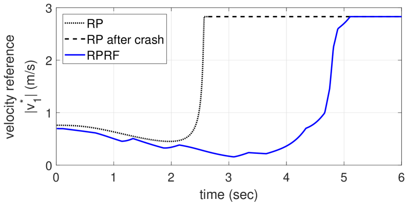
Figure 9: Velocity reference signals with different QP-based controllers.

VI-C Collision Avoidance in the Case of Three Quadrotors

To verify the proposed method in practice, we consider a scenario of three quadrotors swapping positions.

The primary controller is trajectory tracking. The reference trajectories of the agents are generated by sinusoidal functions:

$$p^{r}_{1}(t) =[-\cos(2\pi t/15);-\cos(2\pi t/15);1],$$ (206)

$$p^{r}_{2}(t) =[\cos(2\pi t/15)-0.23;\cos(2\pi t/15)+0.23;1],$$ (207)

$$p^{r}_{3}(t) =[\cos(2\pi t/15)+0.23;\cos(2\pi t/15)-0.23;1].$$ (208)

And the velocity commands are generated by feedforward-feedback controllers:

$$v_{i}^{c}(t)=-1.7(p_{i}(t)-p_{i}^{r}(t))+\dot{p}_{i}^{r}(t)$$ (209)

for $i=1,2,3$.

For both of the algorithms, we choose

$$D =0.2, D_{s} =0.3, \delta =100,$$ (210)

$$\mu(s) =\frac{1}{s+D_{s}}, V(\tilde{p}) =|\tilde{p}|^{-1}, \alpha_{V}(s) =0.3s.$$ (211)

For the QP algorithm with RPRF, we also choose

$$c_{K} =1, c_{P} =1$$ (212)

and $[A_{1}^{r}]_{j,:}=[\cos(2\pi j/n_{p}),~{}\sin(2\pi j/n_{p})]$ for $j=1,\ldots,n_{p}$ with $n_{p}=11$. Accordingly, $c_{A}=\cos(2\pi/11)$.

Figures 10 and 11 show the trajectories of the controlled mobile agents and the norms of the velocity reference signals with the two algorithms. Although collision avoidance is achieved in both of the cases, one may recognize a sudden change of agent 1’s velocity reference signal at $t=4.1$ when the QP-based algorithm without feasible-set reshaping is applied.

Figure 10: Trajectories of the agents with different QP-based controllers.

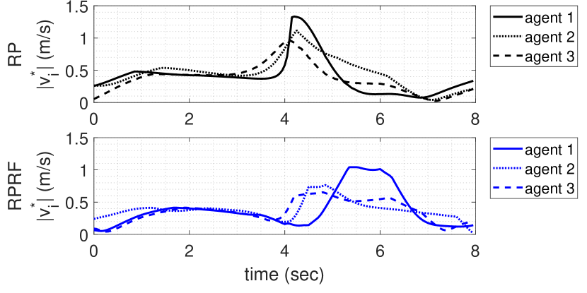
Figure 11: Norms of the velocity reference signals with different QP-based controllers.

VII Conclusions

This paper has developed a systematic solution to the control of safety-critical multi-agent systems subject to uncertain actuation dynamics. The major contribution lies in a seamless integration of a new QP-based design with reshaped feasible set and a nonlinear small-gain analysis. In particular, the new feasible-set reshaping technique has been proved to be quite useful for feasibility of the refined QP algorithm and Lipschitz continuity of its solution. The nonlinear small-gain analysis takes advantage of the interconnection between the controlled nominal system and the uncertain actuation system for ensured safety.

We imagine that the new techniques are beneficial to solving multi-objective control problems for more general systems, e.g., control-affine systems and nonholonomic systems, and control systems subject to information constraints, e.g., partial-state feedback and sampled-data feedback. It is also of theoretical and practical interest to study distributed and coordinated implementations of the algorithms.

Appendix A Technical Lemmas on Linear Spans and Positive Spans

The following two lemmas are used to prove the implementability of the feasible-set reshaping technique proposed in this paper. One may consult [51] for basic notions of positive linear combination. Due to space limitation, the proofs of the lemmas are given in the technical report [42].

Lemma 1

Suppose that any $n$ of the nonzero vectors $v_{1},\ldots,v_{m}\in\mathbb{R}^{n}$ with $m\geq n$ are linearly independent. For any specific $v^{*}\in\mathbb{R}^{n}$ and any positive constant $\epsilon$, one can find a vector $v_{m+1}\in\mathbb{R}^{n}$ such that $|v_{m+1}-v^{*}|\leq\epsilon$ and any $n$ of the vectors $v_{1},\ldots,v_{m+1}$ are linearly independent.

Lemma 2

There exist $v_{1},\ldots,v_{r}\in\mathbb{R}^{n}$ with $r\geq n+1$, any $n$ of which are linearly independent, to positively span $\mathbb{R}^{n}$.

Si Wu received the B.E. degree in Automation from Henan Polytechnic University, China, in 2017, and the M.E. degree in Control Engineering from Northeastern University, China, in 2020. He is pursuing his Ph.D. degree in Control Science and Engineering at Northeastern University. His research interest focuses on nonlinear control theory and applications to vehicles and robotic systems. He was a leading team member winning the IMAV 2019 outdoor competition.

Tengfei Liu received the B.E. degree in automation, in 2005, the M.E. degree in control theory and control engineering, in 2007, both from South China University of Technology, Guangzhou, China, and the Ph.D. degree in engineering from RSISE, the Australian National University, Canberra, Australia, in 2011. From 2011 to 2013, he was a Postdoc with faculty fellowship at Polytechnic Institute of New York University. Since 2014, he has been a Faculty Member with Northeastern University, Shenyang, China. His research interests include stability and control of interconnected nonlinear systems.

Magnus Egerstedt is the Dean of Engineering and a Professor in the Department of Electrical Engineering and Computer Science at the University of California, Irvine. Prior to joining UCI, Egerstedt was on the faculty at the Georgia Institute of Technology. He received the M.S. degree in Engineering Physics and the Ph.D. degree in Applied Mathematics from the Royal Institute of Technology, Stockholm, Sweden, the B.A. degree in Philosophy from Stockholm University, and was a Postdoctoral Scholar at Harvard University. Dr. Egerstedt conducts research in the areas of control theory and robotics, with particular focus on control and coordination of multi-robot systems. Magnus Egerstedt is a Fellow of IEEE and IFAC, and is a Foreign member of the Royal Swedish Academy of Engineering Science. He has received a number of teaching and research awards, including the Ragazzini Award, the O. Hugo Schuck Best Paper Award, the Outstanding Doctoral Advisor Award and the HKN Outstanding Teacher Award from Georgia Tech, and the Alumni of the Year Award from the Royal Institute of Technology.

Zhong-Ping Jiang received the M.Sc. degree in statistics from the University of Paris XI, France, in 1989, and the Ph.D. degree in automatic control and mathematics from the Ecole des Mines de Paris (now, called ParisTech-Mines), France, in 1993, under the direction of Prof. Laurent Praly. Currently, he is a Professor of Electrical and Computer Engineering at the Tandon School of Engineering, New York University. His main research interests include stability theory, robust/adaptive/distributed nonlinear control, robust adaptive dynamic programming, reinforcement learning and their applications to information, mechanical and biological systems. He has served as Deputy Editor-in-Chief, Senior Editor and Associate Editor for numerous journals. Prof. Jiang is a Fellow of the IEEE, a Fellow of the IFAC, a Fellow of the CAA and is among the Clarivate Analytics Highly Cited Researchers. In 2021, he is elected as a foreign member of the Academy of Europe.

References

• [1] J.-C. Latombe, Robot Motion Planning.   Springer, 1991.
• [2] R. C. Arkin, Behavior-Based Robotics.   MIT Press, 1998.
• [3] H. Choset, K. M. Lynch, S. Hutchinson, G. A. Kantor, W. Burgard, L. E. Kavraki, and S. Thrun, Principles of Robot Motion: Theory, Algorithms, and Implementations.   MIT Press, 2005.
• [4] W. Ren and R. W. Beard, Distributed Consensus in Multi-vehicle Cooperative Control: Theory and Applications.   Springer, 2008.
• [5] F. Bullo, J. Cortés, and S. Martinez, Distributed Control of Robotic Networks: A Mathematical Approach to Motion Coordination Algorithms.   Princeton University Press, 2009.
• [6] M. Mesbahi and M. Egerstedt, Graph Theoretic Methods in Multiagent Networks.   Princeton University Press, 2010.
• [7] S. P. Boyd and L. Vandenberghe, Convex Optimization.   Cambridge University Press, 2004.
• [8] E. Polak, T. H. Yang, and D. Q. Mayne, “A method of centers based on barrier functions for solving optimal control problems with continuum state and control constraints,” SIAM Journal on Control and Optimization, vol. 31, pp. 159–179, 1993.
• [9] A. G. Wills and W. P. Heath, “Barrier function based model predictive control,” Automatica, vol. 40, pp. 1415–1422, 2004.
• [10] K. B. Ngo, R. Mahony, and Z. P. Jiang, “Integrator backstepping using barrier functions for systems with multiple state constraints,” in Proceedings of the 44th IEEE Conference on Decision and Control, 2005, pp. 8306–8312.
• [11] K. P. Tee, S. S. Ge, and E. H. Tay, “Barrier Lyapunov functions for the control of output-constrained nonlinear systems,” Automatica, vol. 45, pp. 918–927, 2009.
• [12] P. Wieland and F. Allgower, “Constructive safety using control barrier functions,” in Proceedings of the 7th IFAC Symposium on Nonlinear Control System, 2007, pp. 462–467.
• [13] S. Prajna, A. Jadbabaie, and G. J. Pappas, “A framework for worst-case and stochastic safety verification using barrier certificates,” IEEE Transactions on Automatic Control, vol. 52, pp. 1415–1428, 2007.
• [14] A. D. Ames, J. W. Grizzle, and P. Tabuada, “Control barrier function based quadratic programs with application to adaptive cruise control,” in Proceedings of the 53rd IEEE Conference on Decision and Control, 2014, pp. 6271–6278.
• [15] R. Wisniewski and C. Sloth, “Converse barrier certificate theorems,” IEEE Transactions on Automatic Control, vol. 61, pp. 1356–1361, 2016.
• [16] M. Z. Romdlony and B. Jayawardhana, “Stabilization with guaranteed safety using control Lyapunov–barrier function,” Automatica, vol. 66, pp. 39–47, 2016.
• [17] Z. Artstein, “Stabilization with relaxed controls,” Nonlinear Analysis: Theory, Methods & Applications, vol. 7, pp. 1163–1173, 1983.
• [18] A. D. Ames, X. Xu, J. W. Grizzle, and P. Tabuada, “Control barrier function based quadratic programs for safety critical systems,” IEEE Transactions on Automatic Control, vol. 62, pp. 3861–3876, 2017.
• [19] X. Xu, P. Tabuada, J. W. Grizzle, and A. D. Ames, “Robustness of control barrier functions for safety critical control,” in Proceedings of the 19th IFAC World Congress, 2014, pp. 054–061.
• [20] M. Jankovic, “Robust control barrier functions for constrained stabilization of nonlinear systems,” Automatica, vol. 96, pp. 359–367, 2018.
• [21] E. D. Sontag, “A ‘universal’ construction of Artstein’s theorem on nonlinear stabilization,” Systems & Control Letters, vol. 13, pp. 117–123, 1989.
• [22] R. A. Freeman and P. V. Kokotović, Robust Nonlinear Control Design: State-space and Lyapunov Techniques.   Boston: Birkhäuser, 1996.
• [23] A. Escande, N. Mansard, and P.-B. Wieber, “Hierarchical quadratic programming: Fast online humanoid-robot motion generation,” International Journal of Robotics Research, vol. 33, pp. 1006–1028, 2014.
• [24] D. Mellinger and V. Kumar, “Minimum snap trajectory generation and control for quadrotors,” in Proceedings of the 2011 IEEE International Conference on Robotics and Automation, 2011, pp. 2520–2525.
• [25] A. D. Ames and M. Powell, “Towards the unification of locomotion and manipulation through control Lyapunov functions and quadratic programs,” in Control of Cyber-Physical Systems, D. Tarraf, Ed.   Springer, 2013, pp. 219–240.
• [26] M. Z. Romdlony and B. Jayawardhana, “On the new notion of input-to-state safety,” in Proceedings of the 55th Conference on Decision and Control, 2016, pp. 6403–6409.
• [27] S. Kolathaya and A. D. Ames, “Input-to-state safety with control barrier functions,” IEEE Control Systems Letters, vol. 3, pp. 108–113, 2019.
• [28] P. Ong and J. Cortés, “Universal formula for smooth safe stabilization,” in Proceedings of the 58th IEEE Conference on Decision and Control, 2019, pp. 2373–2378.
• [29] B. J. Morris, M. J. Powell, and A. D. Ames, “Continuity and smoothness properties of nonlinear optimization-based feedback controllers,” in Proceedings of the 54th IEEE Conference on Decision and Control, 2015, pp. 151–158.
• [30] W. S. Cortez, D. Oetomo, C. Manzie, and P. Choong, “Control barrier functions for mechanical systems: Theory and application to robotic grasping,” IEEE Transactions on Control Systems Technology, vol. 29, pp. 530–545, 2021.
• [31] L. Wang, A. D. Ames, and M. Egerstedt, “Safety barrier certificates for collisions-free multirobot systems,” IEEE Transactions on Robotics, vol. 33, pp. 661–674, 2017.
• [32] P. Glotfelter, J. Cortes, and M. Egerstedt, “Nonsmooth barrier functions with applications to multi-robot systems,” IEEE Control Systems Letters, vol. 1, pp. 310–315, 2017.
• [33] S. Wilson, P. Glotfelter, L. Wang, S. Mayya, G. Notomista, M. Mote, and M. Egerstedt, “The robotarium: Globally impactful opportunities, challenges, and lessons learned in remote-access, distributed control of multirobot systems,” IEEE Control Systems Magazine, vol. 40, pp. 26–44, 2020.
• [34] A. Ames, S. Coogan, M. Egerstedt, G. Notomista, K. Sreenath, and P. Tabuada, “Control barrier functions: Theory and applications,” in Proceedings of the 18th European Control Conference, 2019, pp. 3420–3431.
• [35] P. Fiorini and Z. Shiller, “Motion planning in dynamic environments using velocity obstacles,” International Journal of Robotics Research, vol. 17, pp. 760–772, 1998.
• [36] J. van den Berg, S. J. Guy, M. Lin, and D. Manocha, “Reciprocal $n$-body collision avoidance,” in Robotics Research, B. Siciliano, O. Khatib, and F. Groen, Eds.   Springer-Verlag, 2011, pp. 3–19.
• [37] M. Rufli, J. Alonso-Mora, and R. Siegwart, “Reciprocal collision avoidance with motion continuity constraints,” IEEE Transactions on Robotics, vol. 29, no. 4, pp. 899–912, 2013.
• [38] A. Singletary, K. Klingebiel, J. Bourne, A. Browning, P. Tokumaru, and A. Ames, “Comparative analysis of control barrier functions and artificial potential fields for obstacle avoidance,” in Proceedings of the 2021 IEEE/RSJ International Conference on Intelligent Robots and Systems.   IEEE, 2021, pp. 8129–8136.
• [39] O. Khatib, “Real-time obstacle avoidance for manipulators and mobile robots,” International Journal of Robotics Research, vol. 5, pp. 90–98, 1986.
• [40] Z. P. Jiang, A. R. Teel, and L. Praly, “Small-gain theorem for ISS systems and applications,” Mathematics of Control, Signals, and Systems, vol. 7, pp. 95–120, 1994.
• [41] E. D. Sontag, “Input to state stability: Basic concepts and results,” in Nonlinear and Optimal Control Theory, P. Nistri and G. Stefani, Eds.   Berlin: Springer-Verlag, 2008, pp. 163–220.
• [42] S. Wu, T. Liu, M. Egerstedt, and Z. P. Jiang, “Quadratic programming for continuous control of safety-critical multi-agent systems under uncertainty,” Northeastern University, Tech. Rep., 2021, http://faculty.neu.edu.cn/liutengfei/en/zdylm/309596/list/index.htm.
• [43] H. K. Khalil, Nonlinear Systems, 3rd ed.   NJ: Prentice-Hall, 2002.
• [44] T. Liu, Z. P. Jiang, and D. J. Hill, Nonlinear Control of Dynamic Networks.   FL: CRC Press, 2014.
• [45] Z. P. Jiang and T. Liu, “Small-gain theory for stability and control of dynamical networks: A survey,” Annual Reviews in Control, vol. 46, pp. 58–79, 2018.
• [46] P. Glotfelter, I. Buckley, and E. Magnus, “Hybrid nonsmooth barrier functions with applications to provably safe and composable collision avoidance for robotic systems,” IEEE Robotics and Automation Letters, vol. 4, no. 2, pp. 1303–1310, 2019.
• [47] E. Sontag and Y. Wang, “Lyapunov characterizations of input to output stability,” SIAM Journal on Control and Optimization, vol. 39, pp. 226–249, 2000.
• [48] D. Fox, W. Burgard, and S. Thrun, “The dynamic window approach to collision avoidance,” IEEE Robotics & Automation Magazine, vol. 4, pp. 23–33, 1997.
• [49] D. P. Bertsekas, Nonlinear Programming, 2nd ed.   Athena Scientific, 1999.
• [50] W. W. Hager, “Lipschitz continuity for constrained processes,” SIAM Journal on Control and Optimization, vol. 17, pp. 321–338, 1979.
• [51] C. Davis, “Theory of positive linear dependence,” American Journal of Mathematics, vol. 76, pp. 733–746, 1954.
• [52] R. A. Horn and C. R. Johnson, Matrix Analysis.   Cambridge University Press, 2012.
• [53] K. G. Binmore, Mathematical Analysis: A Straightforward Approach.   Cambridge University Press, 1982.