Analysis of UAV Radar and Communication Network Coexistence with Different Multiple Access Protocols

Abstract

Unmanned aerial vehicles (UAVs) are expected to be used extensively in the future for various applications, either as user equipment (UEs) connected to a cellular wireless network, or as an infrastructure extension of an existing wireless network to serve other UEs. Next generation wireless networks will consider the use of UAVs for joint communication and radar and/or as dedicated radars for various sensing applications. Increasing number of UAVs will naturally result in larger number of communication and/or radar links that may cause interference to nearby networks, exacerbated further by the higher likelihood of line-of-sight signal propagation from UAVs even to distant receivers. With all these, it is critical to study network coexistence of UAV-mounted base stations (BSs) and radar transceivers. In this paper, using stochastic geometry, we derive closed-form expressions to characterize the performance of coexisting UAV radar and communication networks for spectrum overlay multiple access (SOMA) and time-division multiple access (TDMA). We evaluate successful ranging probability (SRP) and the transmission capacity (TC) and compare the performance of TDMA and SOMA. Our results show that SOMA can outperform TDMA on both SRP and TC when the node density of active UAV-radars is larger than the node density of UAV-comms.

I Introduction

Recently, various different applications of cellular-connected unmanned aerial vehicles (UAVs) have been getting significant attention due to their cost-efficient deployment and controllable mobility. UAVs are utilized in many fields such as environmental monitoring and surveillance [1], public safety [2], video broadcasting [3], and delivery [4]. Moreover, UAV-mounted base stations (UAV-BS) and user equipment (UAV-UE), as well as UAV-mounted radars (UAV-radar) are commonly considered in sensing and communication applications, since the UAVs are available to quickly change the position to serve users at the outage area, and/or surveil/track the location of detected moving targets. Joint design of the radar and communication systems is considered as one of the key research areas for wireless networks beyond 5G systems which can benefit significantly from the use of autonomous UAVs.

In the meanwhile, as the demand for using wider bandwidths has been increasing to support higher throughput and massive connectivity, the band of operation for broadband wireless networks has been moving to higher frequencies such as millimeter-wave (mmWave) and sub/THz bands that are also commonly used by radar systems. Some traditional radar bands, including certain bands below 6 GHz, are also being opened for shared use with communication networks due to the increasing congestion in the dedicated spectrum for cellular networks. All these developments call for rigorously studying the coexistence scenarios for radar and communication networks and coming up with strategies for effective spectrum sharing [5].

Stochastic geometry-based techniques are commonly used in the literature for obtaining closed-form expressions on the performance of wireless networks where transmit sources are randomly deployed in the spatial domain [6]. For example, the analysis of accumulated interference from multiple nodes following a homogeneous Poisson point process (HPPP) is useful to evaluate the capacity of wireless networks [6]. In this paper, we specifically investigate UAV radar sensing and communication network coexistence scenarios. In particular, we consider scenarios where radar transmission and data transmission are coordinated by two different multiple-access protocols: spectrum overlay multiple access (SOMA) and time-division multiple access (TDMA). In SOMA, radar sensing and data communication share the same spectrum so that the spectrum is overlapped. On the other hand, in TDMA, radar detection and communication are separated by time. We utilize stochastic geometry-based analysis where UAVs are randomly located in 3D space following a two-dimensional homogeneous Poisson point process (HPPP). We individually analyze the radar detection performance and the data communication performance using the successful ranging probability (SRP) and the transmission capacity (TC), respectively.

Table I: Literature review for stochastic geometry based wireless network performance analysis.

Ref.	Analysis objective	Application	Radar	Networks
[7]	TC with different spatial diversity techniques	Terrestrial	✗	Ad hoc
[8]	Information and energy outage probability and area harvested energy	Terrestrial	✗	SWIPT in ad hoc networks
[9]	Channel outage and packet loss probability	Terrestrial	✗	DL URLLC communications
[10, 11]	SRP	Terrestrial	✓	Radar with road scenario
[12]	SRP	Terrestrial	✓	Radar networks
[13, 14]	Coverage probability with different antenna patterns and directivity	Terrestrial	✗	DL cellular
[15]	Connection and secrecy probability	Terrestrial	✗	DL secure communication cellular
[16]	Coverage probability with underlay and overlay protocols	UAV	✗	UAV-to-UAV and UL terrestrial
[17]	Coverage probability and spectral efficiency	UAV	✗	Two-tiers cellular
[18, 19]	Coverage probability and spectral efficiency	UAV	✗	DL communication
[20]	Successful transmission probability, energy and SINR coverage	UAV	✗	DL SWIPT and UL communication
[21]	Coverage probability	UAV	✗	UAV-aided DL and UL communication
[22]	LoS probability	UAV	✗	BS-to-UAV link
[23]	Coverage probability, motion energy, and flight time	UAV	✗	UAV path planning
[24]	Connection, secrecy, and energy-information outage probability	UAV	✗	Secure communication in SWIPT
This work	SRP and TC	UAV	✓	Radar and communication coexistence

Contributions of this paper can be summarized as follows:

• We derive closed-form expressions for SRP and TC on the UAV radar and communication coexistence scenario where UAVs are placed following HPPP with a guard zone.

• We analyze the performance of SRP and TC in SOMA and TDMA, respectively. We also investigate behaviors of SRP and TC depending on the node density, radius of the guard zone, power splitting factor in SOMA, and time division factor in TDMA.

• We analytically compare TDMA and SOMA on SRP and TC and show that TDMA outperforms SOMA on SRP while SOMA is better than TDMA on TC in the general condition. Furthermore, we analyze the condition that SOMA can be superior to TDMA on both SRP and TC metrics.

The rest of this paper is organized as follows. Section II presents the literature review. In Section III, we describe the UAV radar and communication network coexistence design. In Section IV, we provide the signal propagation model when UAVs are distributed by HPPP. In Section V, we derive the closed-form expressions of the SRP and the TC. In Section VI, we analyze SRP depending on the system parameters and the multiple access protocols. In Section VII, we analyze the TC depending on the system parameters and the multiple access protocols. In Section VIII, we compare the SRP and the TC performance of SOMA and TDMA. In Section IX, we show the simulation results to verify the analysis in previous sections, and Section X provides concluding remarks.

II Literature Review

The operation of UAVs on BSs and radar detectors have been investigated in the literature. A flying UAV-BS can maximize the capacity or minimize the outage of networks by optimizing UAV trajectory [25, 26]. In [27, 28], the trajectory and precoder of UAV-BS are optimized to maximize physical layer secrecy. In [29], a UAV-radar is used in measuring the depth of the snow on the sea. Human detection and classification by a UAV-radar have been studied in [30]. Target detection using radar imaging from UAV-radar has been investigated in [31]. In [32], the feasibility of a surveillance system using a UAV-radar has been explored.

The study of coexistence networks has been explored in the literature. In [33], a beamforming approach has been studied to facilitate the coexistence between downlink (DL) multi-user-multiple-input-multiple-output (MU-MIMO) communication and MIMO radar system. In [34], the joint design of the radar and communication system for the coexistence of MIMO radar and MIMO communication has been studied. Moreover, UAV communication and radar sensing network coexistence that utilizes the spectrum for both purposes has been investigated for an efficient and flexible system design [35]. In [36], joint UAV communication and cooperative sensing network based on beam sharing scheme has been explored.

Stochastic geometry based network analysis has been thoroughly investigated in the literature. TC is analyzed in ad hoc networks with different spatial diversity techniques where transmitting nodes are distributed by an HPPP [7], and this work is extended to the wireless information and power transfer (SWIPT)-based ad hoc networks in [8]. In [9], packet loss probability depending on the packet size, packet duration, and SINR are derived in downlink ultra-reliable and low-latency communications (URLLC) scenarios where distributed antenna ports are randomly placed following an HPPP. In [10, 11, 12], the effect of radar interference on the radar detection performance is analyzed and SRP is evaluated using stochastic geometry. More specifically, the geometric layout of vehicles on a road where the locations of vehicles on a certain lane are decided by unidimensional HPPP model is investigated in [10, 11]. In [11], radar cross-section (RCS) characteristics are modeled and analyzed using HPPPs for automotive radar network scenarios. In [13, 14], the effects of different directional antenna patterns, node densities, and antenna array sizes on coverage probability are studied for mmWave networks. The locations of BSs and the eavesdroppers are randomly distributed by independent HPPPs in [15], and closed-form expression of secrecy probability for secure communications is explored.

Closed-form analysis of network performance using stochastic geometry techniques have also been studied in UAV networks in [16, 17, 18, 19, 20, 21, 22, 23, 24]. In [16], coexisting UAV-to-UAV links and uplink (UL) ground-BS to ground-user links are considered. Then, coverage of two different scenarios are studied, where the spectrum for each link is either reused, or it is allocated in a dedicated manner. The literature review with representative works related to stochastic geometry-based wireless network performance analysis is summarized in Table I. To the best of our knowledge, the study of radar networks based on stochastic geometry has been limited, and UAV communication and radar network coexistence scenario has not been investigated yet.

Table II: Key symbols and notations used in this paper.

Symbol	Definition
${\lambda_{\rm r}}^{\prime}$	Node density of UAV-radars
${\lambda_{\rm d}}^{\prime}$	Node density of UAV-comms
${\bar{\lambda}}_{\rm r}$	Active node density of UAV-radars
${\lambda_{\rm r}}$	Effective node density of active UAV-radars in HPPP
${\lambda_{\rm d}}$	Effective node density of UAV-comms in HPPP
$\mathsf{h}_{\rm UAV}$	UAVs height
$r_{0}$	Radius of guard zone
$\phi$	Power splitting factor
$\tau$	Time division factor
$\delta$	Duty circle
$\mathsf{P}_{\rm Tx}$	Transmit power
$\mathsf{G}_{\rm t}$	Tx antenna gain
$\alpha$	Path-loss exponent
$\alpha_{\rm I}$	Path-loss exponent from the interference
$\mathsf{G}_{\rm r}$	Receiver antenna gain
$\mathsf{G}_{\rm rI}$	Receiver antenna gain from the interference
$\bar{\sigma}$	Average RCS
$\sigma$	RCS
$S_{\rm e}$	Effective aperture of radar receiver
$\mathsf{G}_{\rm p}$	Processing gain of radar receiver
$f_{\rm c}$	Carrier frequency
$R_{0}$	Target distance
$r_{i}$	Distance from the interferer
$c$	Speed of light
$h_{0}$	Small-scale fading
$h_{i}$	Small-scale fading from the interference
$\beta_{\rm th}$	Target SINR threshold for outage probability
$\gamma{\rm th}$	Target SINR threshold for successful range probability
$\beta_{0}$	SINR of the received data signal
$\gamma{0}$	SINR of the received radar signal
$N_{0}$	Noise power

III System Model

We consider UAV networks where radar nodes and communication nodes coexist. Radar-mounted UAVs (UAV-radars) detect and track a target on the ground by transmitting radar signals and receiving the reflected signals from the target. On the other hand, UAVs that are equipped with a BS (UAV-comms) communicate with a ground user. We assume that UAV-radars and UAV-comms follow a two-dimensional HPPP independently where the node densities are ${\lambda_{\rm r}}^{\prime}$ and ${\lambda_{\rm d}}^{\prime}$ respectively. All UAVs fly at a fixed identical height $\mathsf{h}_{\rm UAV}$. Fig. 1 describes two different network representations of the radar detection scenario and the communication scenario in the HPPP model. The guard zone with radius $r_{0}$ is considered between two UAVs, or between a UAV and a user to protect them from potential strong interference. The distance between a UAV-radar and a target in the radar detection scenario and the distance between a UAV-comm and a served user in the communication scenario is $R_{0}$. UAV-radars are assigned to active UAV-radar by the random spectrum access with the duty cycle $\delta$, and the rest of UAV-radars remain inactive UAV-radars in the networks.

(a)

(b)

Figure 1: UAV radar and communication network coexistence. A blue UAV is either: (a) a typical UAV-radar that detects a target using radar transmission; or (b) a serving UAV that communicates with a typical user. The green UAV-comms or the red (active) UAV-radars can interfere with radar detection or communication signals. The black (inactive) UAV-radars do not transmit any interference signals. To avoid strong interference, a guard zone is with a radius $r_{0}$ established between UAVs, and between a UAV and a user.

Figure 2: Two different multiple access schemes: SOMA (left) and TDMA (right).

In the radar and communication coexistence, UAV-radars and UAV-comms need to coordinate the time and spectrum resources for radar and data transmissions. We consider two different multiple access schemes: SOMA where radar signal and data signal share the same spectrum during transmission time, and TDMA where the time for radar and data transmission is scheduled at separate time slots. Fig. 2 illustrates different radar and data allocations depending on multiple access schemes. The power allocated to radar and communication is determined by power splitting factor $\phi$ for SOMA, and the time duration assigned to radar and communication is decided by time division factor $\tau$ for TDMA. Note that the interference behavior in this network coexistence is dependent on the multiple access. In this paper, we focus on the analysis and comparison of SOMA and TDMA on data transmission and radar detection. The key parameters are summarized in Table II.

IV Signal Propagation Models in HPPP

In this section, we describe signal and interference models in HPPP when SOMA and TDMA are adopted respectively. Throughout this paper, we denote SOMA and TDMA as $\rm s.o.$ and $\rm t.d.$ at the superscript.

IV-A Radar and Data Signal Models

IV-A1 SOMA

We place a typical UAV-radar with the origin $(0,\leavevmode\nobreak\ 0,\leavevmode\nobreak\ \mathsf{h}_{\rm UAV})$ and distance from the target at $(x_{\rm t},y_{\rm t},0)$ is $R_{0}=\sqrt{x_{\rm t}^{2}+y_{\rm t}^{2}+(\mathsf{h}_{\rm UAV})^{2}}$ as in Fig. 1(a). We assume that the height of a UAV-radar $\mathsf{h}_{\rm UAV}$ is sufficiently high so that line-of-sight is secured to detect the target and the free-space path loss model can be considered [37]. The power of the received signal that is reflected back from the target can be expressed as [10],

$$\mathsf{P}_{\rm r}^{\rm s.o.}=\left(\frac{(1-\phi)\mathsf{P}_{\rm Tx}\mathsf{G}_{\rm t}}{4\pi R_{0}^{\alpha}}\right)\left(\frac{\sigma S_{\rm e}}{4\pi R_{0}^{\alpha}}\right)\mathsf{G}_{\rm p},$$ (1)

where $\mathsf{P}_{\rm Tx}$, $\mathsf{G}_{\rm t}$, $\alpha$ indicate transmit power, Tx antenna gain, and path loss exponent, and $\sigma$, $S_{\rm e}$, $\mathsf{G}_{\rm p}$ denote radar cross-section (RCS) of the target, the effective aperture of radar receiver, and the processing gain. Swerling I model is considered for the RCS and the RCS of the target follows the exponential distribution, $\sigma\sim\frac{1}{\bar{\sigma}}e^{-\frac{\sigma}{\bar{\sigma}}}$ [11]. The effective area is given by

$$S_{\rm e}=\frac{\mathsf{G}_{\rm r}c^{2}}{4\pi f_{\rm c}^{2}},$$ (2)

where $c$, $f_{\rm c}$ denote the speed of light and the carrier frequency. Then, the power of the reflected back radar signal in (1) can be rewritten as

$$\mathsf{P}_{\rm r}^{\rm s.o.}=\frac{(1-\phi)\mathsf{P}_{\rm Tx}\mathsf{G}_{\rm t}\mathsf{G}_{\rm r}\mathsf{G}_{\rm p}c^{2}\sigma}{(4\pi)^{3}f_{\rm c}^{2}R_{0}^{2\alpha}}.$$ (3)

In the communication scenario as in Fig. 1(b), a typcial user is located at the origin and it receives the signal from the serving UAV-comm at $(x_{\rm t},y_{\rm t},\mathsf{h}_{\rm UAV})$, which is at a distance of $R_{0}=\sqrt{x_{\rm t}^{2}+y_{\rm t}^{2}+(\mathsf{h}_{\rm UAV})^{2}}$ from the user. The power of the received signal of the user is given by

$$\mathsf{P}_{\rm d}^{\rm s.o.}=\frac{\phi\mathsf{P}_{\rm Tx}\mathsf{G}_{\rm t}\mathsf{G}_{\rm r}c^{2}}{(4\pi)^{2}f_{\rm c}^{2}R_{0}^{\alpha}}h_{0},$$ (4)

where $h_{0}\sim\exp(1)$ represents Rayleigh small-scale fading. Note that the allocated power of the radar and the data signals are split by the power splitting factor $\phi$ in SOMA as illustrated in Fig 2.

IV-A2 TDMA

The received signal power of the radar signal and the data signal in TDMA are expressed as

$$\mathsf{P}_{\rm r}^{\rm t.d.}=\frac{\mathsf{P}_{\rm Tx}\mathsf{G}_{\rm t}\mathsf{G}_{\rm r}\mathsf{G}_{\rm p}c^{2}\sigma}{(4\pi)^{3}f_{\rm c}^{2}R_{0}^{2\alpha}},$$ (5)

$$\mathsf{P}_{\rm d}^{\rm t.d.}=\frac{\mathsf{P}_{\rm Tx}\mathsf{G}_{\rm t}\mathsf{G}_{\rm r}c^{2}}{(4\pi)^{2}f_{\rm c}^{2}R_{0}^{\alpha}}h_{0}.$$ (6)

Since the radar detection and communication are separately conducted in different time slots in TDMA, transmit power is not adjusted as in SOMA.

IV-B Effective Radar and Communication Node Densities

The PPP in this network introduces the guard zone and it can be modeled by the Matérn hard-core point processes (MHCPP) type-II, which can be further approximated by the HPPP model.

IV-B1 SOMA

The approximated effective node density of the radar and the communication from MHCPP type-II can be written as [38]

$$\lambda_{\rm r}^{\rm s.o.}=\frac{1-e^{-\bar{\lambda}_{\rm r}^{\rm s.o.}\pi r_{0}^{2}}}{\pi r_{0}^{2}},\leavevmode\nobreak\ \lambda_{\rm d}^{\rm s.o.}=\frac{1-e^{-\lambda^{\prime}_{\rm d}\pi r_{0}^{2}}}{\pi r_{0}^{2}},$$ (7)

where ${\bar{\lambda}}_{\rm r}^{\rm s.o.}=\delta\lambda^{\prime}_{\rm r}$ is the active UAV-radar node density, and $\delta$ is the duty cycle.

IV-B2 TDMA

The effective node density of the radar and the communication from MHCPP type-II can be written as

$$\lambda_{\rm r}^{\rm t.d.}=\frac{1-e^{-\bar{\lambda}^{\rm t.d.}_{\rm r}\pi r_{0}^{2}}}{\pi r_{0}^{2}},\leavevmode\nobreak\ \lambda_{\rm d}^{\rm t.d.}=\frac{1-e^{-\lambda^{\prime}_{\rm d}\pi r_{0}^{2}}}{\pi r_{0}^{2}},$$ (8)

where ${\bar{\lambda}}_{\rm r}^{\rm t.d.}=\frac{\delta}{1-\tau}\lambda^{\prime}_{\rm r}$ is the active UAV-radar node density. Note that the duty cycle $\delta$ in SOMA increases to $\frac{\delta}{1-\tau}$ in TDMA as much as the reduced radar transmission time by $\tau$, since it is assumed that the total number of active UAV-radar nodes during the time period is the same for both SOMA and TDMA. Since the effective node density of UAV-comms for TDMA and SOMA is equal, we merge the notation of the node density as $\lambda_{\rm d}=\lambda_{\rm d}^{\rm s.o.}=\lambda_{\rm d}^{\rm t.d.}$.

IV-C Interference Models

In this subsection, we obtain the power of interference coming from nearby active UAV-radars and UAV-comms in the HPPP model.

IV-C1 SOMA

Since the radar detection and communication occupy the same spectrum band at the same time, the aggregated interference power from UAV-radars and UAV-comms can be expressed as

$$\mathsf{I}^{\rm s.o.} =\underbrace{\sum_{r_{i}\in\Phi(\lambda_{\rm d})\backslash r_{0}}\frac{\phi\mathsf{P}_{\rm Tx}\mathsf{G}_{\rm t}\mathsf{G}_{\rm rI}c^{2}}{(4\pi)^{2}f_{\rm c}^{2}r_{i}^{\alpha_{\rm I}}}h_{i}}_{\text{interfence from nearby UAV-comms }(\mathsf{I}_{1})}$$

$$+\underbrace{\sum_{r_{j}\in\Phi(\lambda_{\rm r}^{\rm s.o.})\backslash r_{0}}\frac{(1-\phi)\mathsf{P}_{\rm Tx}\mathsf{G}_{\rm t}\mathsf{G}_{\rm rI}c^{2}}{(4\pi)^{2}f_{\rm c}^{2}r_{j}^{\alpha_{\rm I}}}h_{j}}_{\text{interfence from nearby UAV-radars }(\mathsf{I}_{2})},$$ (9)

where $r\in\Phi(\lambda)\backslash r_{0}$ means a two-dimensional HPPP with a density $\lambda$ and $r>r_{0}$, $\mathsf{G}_{\rm rI}$ and $\alpha_{\rm I}$ are Rx antenna gain and path-loss exponent from the interfering signals, respectively, $h_{i}$, $h_{j}$ represent small-scale fading from the interference, and $r_{i}$, $r_{j}$ are distance between a typical UAV-radar or user and an interferer. Since the radar detection and communication are carried out together in SOMA, the interference power at both the typical UAV-radar (Fig. 1(a)) and the typical information receiver (Fig. 1(b)) is the same: $\mathsf{I}^{\rm s.o.}=\mathsf{I}^{\rm s.o.}_{\rm d}=\mathsf{I}^{\rm s.o.}_{\rm r}$.

IV-C2 TDMA

The interfence comes only from the UAV-radars in the radar detection scenario. Likewise, the interference comes only from UAV-comms in communication scenario. Then the aggregated interference power for each case can be expressed as

$$\mathsf{I}^{\rm t.d.}_{\rm r} =\sum_{r_{i}\in\Phi(\lambda_{\rm r}^{\rm t.d.})\backslash r_{0}}\frac{\mathsf{P}_{\rm Tx}\mathsf{G}_{\rm t}\mathsf{G}_{\rm rI}c^{2}}{(4\pi)^{2}f_{\rm c}^{2}r_{i}^{\alpha_{\rm I}}}h_{i},$$ (10)

$$\mathsf{I}^{\rm t.d.}_{\rm d} =\sum_{r_{i}\in\Phi(\lambda_{\rm d})\backslash r_{0}}\frac{\mathsf{P}_{\rm Tx}\mathsf{G}_{\rm t}\mathsf{G}_{\rm rI}c^{2}}{(4\pi)^{2}f_{\rm c}^{2}r_{i}^{\alpha_{\rm I}}}h_{i}.$$ (11)

V Performance Analysis of Radar Detection and Data Communication

In this section, we discuss performance evaluation metrics for two different scenarios. Specifically, we derive the SRP in the radar detection scenario and the TC in the communication scenario.

V-A Successful Ranging Probability

SRP is the probability that a UAV-radar succeeds in detecting the target, which is decided by the signal-to-interference-plus-noise ratio (SINR). SRP is defined by

$$\mathsf{Pr_{s.r.}}(\gamma_{\rm th})=\mathsf{Pr}(\gamma_{0}>\gamma_{\rm th}),$$ (12)

where $\gamma_{0}=\frac{\mathsf{P}_{\rm r}}{\mathsf{I}_{\rm r}+\mathsf{N}_{0}}$ and $\mathsf{N}_{0}$ are SINR of the received radar signal and the noise power, respectively. In addition, $\gamma_{\rm th}$ denotes SINR threshold where the target is successfully detected. In what follows, we derive the closed-form expression of SRP in both SOMA and TDMA.

V-A1 SOMA

SRP in (12) can be derived from (3), (IV-C1) as follows:

$$\mathsf{Pr_{s.r.}^{\rm s.o.}}(\gamma_{\rm th})=\mathsf{Pr}\left(\frac{\mathsf{P}^{\rm s.o.}_{\rm r}}{\mathsf{I}^{\rm s.o.}+\mathsf{N}_{0}}>\gamma_{\rm th}\right)$$

$$=\mathsf{Pr}\left(\frac{(1-\phi)\mathsf{P}_{\rm Tx}\mathsf{G}_{\rm t}\mathsf{G}_{\rm r}\mathsf{G}_{\rm p}c^{2}\sigma}{\mathsf{I}^{\rm s.o.}+\mathsf{N}_{0}}>(4\pi)^{3}f_{\rm c}^{2}R_{0}^{2\alpha}\gamma_{\rm th}\right)$$

$$\approx\mathsf{Pr}\left(\sigma>\frac{(4\pi)^{3}f_{\rm c}^{2}R_{0}^{2\alpha}\gamma_{\rm th}\mathsf{I}^{\rm s.o.}}{(1-\phi)\mathsf{P}_{\rm Tx}\mathsf{G}_{\rm t}\mathsf{G}_{\rm r}\mathsf{G}_{\rm p}c^{2}}\right)$$

$$=\int_{0}^{\infty}\left\{1-F_{\sigma}\left(\frac{(4\pi)^{3}f_{\rm c}^{2}R_{0}^{2\alpha}\gamma_{\rm th}y}{(1-\phi)\mathsf{P}_{\rm Tx}\mathsf{G}_{\rm t}\mathsf{G}_{\rm r}\mathsf{G}_{\rm p}c^{2}}\right)\right\}f_{\mathsf{I}^{\rm s.o.}}(y){\rm d}y$$

$$=\int_{0}^{\infty}e^{-\frac{(4\pi)^{3}f_{\rm c}^{2}R_{0}^{2\alpha}\gamma_{\rm th}y}{(1-\phi)\mathsf{P}_{\rm Tx}\mathsf{G}_{\rm t}\mathsf{G}_{\rm r}\mathsf{G}_{\rm p}c^{2}\bar{\sigma}}}f_{\mathsf{I}^{\rm s.o.}}(y){\rm d}y$$

$$=\mathcal{L}_{\mathsf{I}^{\rm s.o.}}\left(\frac{(4\pi)^{3}f_{\rm c}^{2}R_{0}^{2\alpha}\gamma_{\rm th}}{(1-\phi)\mathsf{P}_{\rm Tx}\mathsf{G}_{\rm t}\mathsf{G}_{\rm r}\mathsf{G}_{\rm p}c^{2}\bar{\sigma}}\right)$$ (13)

where the approximation comes from the interference limit regime assumption, $F_{\sigma}(X)=1-e^{-\frac{X}{\bar{\sigma}}}$ is the cumulative distribution function (CDF) of $\sigma$, and $f_{\mathsf{I}^{\rm s.o.}}(\rm x)$ is the probability density function (PDF) of $\mathsf{I}^{\rm s.o.}$, $\mathcal{L}_{\mathsf{I}^{\rm s.o.}}(z)$ indicates Laplace transform of the PDF of $\mathsf{I}^{\rm s.o.}$.

$\mathcal{L}_{\mathsf{I}^{\rm s.o.}}(z)$ can be derived as follows. The interference term can be rewritten as $\mathsf{I}^{\rm s.o.}=\mathsf{I}_{1}+\mathsf{I}_{2}$ where $\mathsf{I}_{1}$, $\mathsf{I}_{2}$ are the first and the second terms in (IV-C1) respectively. Then, we can obtain [9]

$$\mathcal{L}_{\mathsf{I}_{1}}(z) =\exp{\left\{-2\pi\lambda_{\rm d}{\rm A}_{1}(z)\frac{(z\phi{\rm K}_{1})^{\frac{2}{\alpha_{\rm I}}}}{\alpha_{\rm I}}\right\}},$$

$$\mathcal{L}_{\mathsf{I}_{2}}(z) =\exp{\left\{-2\pi\lambda_{\rm r}^{\rm s.o.}{\rm A}_{2}(z)\frac{(z(1-\phi){\rm K}_{1})^{\frac{2}{\alpha_{\rm I}}}}{\alpha_{\rm I}}\right\}},$$ (14)

where ${\rm A}_{1}(z)={\rm B}\left(\frac{2}{\alpha_{\rm I}},1-\frac{2}{\alpha_{\rm I}}\right)-{\rm B}\left(\frac{1}{1+z\phi{\rm K}_{1}r_{0}^{-\alpha_{\rm I}}};\frac{2}{\alpha_{\rm I}},1-\frac{2}{\alpha_{\rm I}}\right)$, ${\rm A}_{2}(z)={\rm B}\left(\frac{2}{\alpha_{\rm I}},1-\frac{2}{\alpha_{\rm I}}\right)-{\rm B}\left(\frac{1}{1+z(1-\phi){\rm K}_{1}r_{0}^{-\alpha_{\rm I}}};\frac{2}{\alpha_{\rm I}},1-\frac{2}{\alpha_{\rm I}}\right)$, ${\rm K_{1}}=\frac{\mathsf{P}_{\rm Tx}\mathsf{G}_{\rm t}\mathsf{G}_{\rm rI}c^{2}}{(4\pi)^{2}f_{\rm c}^{2}}$, ${\rm B}(a,b)$ is the beta function, and ${\rm B}(x;a,b)=\int_{0}^{x}u^{a-1}(1-u)^{b-1}{\rm d}u$ is the incomplete beta fucntion. Then, we can derive

$$\mathcal{L}_{\mathsf{I}^{\rm s.o.}}(z)=\mathcal{L}_{\mathsf{I}_{1}}(z)\mathcal{L}_{\mathsf{I}_{2}}(z)=$$

$$\exp{\left\{-2\pi\left(\phi^{\frac{2}{\alpha_{\rm I}}}\lambda_{\rm d}{\rm A}_{1}(z)+\left(1-\phi\right)^{\frac{2}{\alpha_{\rm I}}}\lambda_{\rm r}^{\rm s.o.}{\rm A}_{2}(z)\right)\frac{(z{\rm K}_{1})^{\frac{2}{\alpha_{\rm I}}}}{\alpha_{\rm I}}\right\}}.$$ (15)

Then, the closed-form expression of SRP in SOMA can be obtained as (V-A1) at the top of the next page.

$$\mathsf{Pr_{s.r.}^{\rm s.o.}}(\gamma_{\rm th})=\exp\left\{-2\pi\left(\left(\frac{\phi}{1-\phi}\right)^{\frac{2}{\alpha_{\rm I}}}\lambda_{\rm d}\underbrace{\left\{{\rm B}\left(\frac{2}{\alpha_{\rm I}},1-\frac{2}{\alpha_{\rm I}}\right)-{\rm B}\left(\frac{1}{1+\left(\frac{\phi 4\pi{\rm G}_{\rm rI}R_{0}^{2\alpha}\gamma_{\rm th}}{(1-\phi)\mathsf{G}_{\rm r}\mathsf{G}_{\rm p}\bar{\sigma}}\right)r_{0}^{-\alpha_{\rm I}}};\frac{2}{\alpha_{\rm I}},1-\frac{2}{\alpha_{\rm I}}\right)\right\}}_{C_{1}}+\right.\right.$$

$$\left.\left.\lambda_{\rm r}^{\rm s.o.}\underbrace{\left\{{\rm B}\left(\frac{2}{\alpha_{\rm I}},1-\frac{2}{\alpha_{\rm I}}\right)-{\rm B}\left(\frac{1}{1+\left(\frac{4\pi{\rm G}_{\rm rI}R_{0}^{2\alpha}\gamma_{\rm th}}{\mathsf{G}_{\rm r}\mathsf{G}_{\rm p}\bar{\sigma}}\right)r_{0}^{-\alpha_{\rm I}}};\frac{2}{\alpha_{\rm I}},1-\frac{2}{\alpha_{\rm I}}\right)\right\}}_{C_{2}}\right)\frac{\left(\frac{4\pi{\rm G}_{\rm rI}R_{0}^{2\alpha}\gamma_{\rm th}}{\mathsf{G}_{\rm r}\mathsf{G}_{\rm p}\bar{\sigma}}\right)^{\frac{2}{\alpha_{\rm I}}}}{\alpha_{\rm I}}\right\}$$ (16)

$$\mathsf{Pr_{s.r.}^{\rm t.d.}}(\gamma_{\rm th})=\exp\left\{-2\pi\lambda_{\rm r}^{\rm t.d.}\underbrace{\left\{{\rm B}\left(\frac{2}{\alpha_{\rm I}},1-\frac{2}{\alpha_{\rm I}}\right)-{\rm B}\left(\frac{1}{1+\left(\frac{4\pi{\rm G}_{\rm rI}R_{0}^{2\alpha}\gamma_{\rm th}}{\mathsf{G}_{\rm r}\mathsf{G}_{\rm p}\bar{\sigma}}\right)r_{0}^{-\alpha_{\rm I}}};\frac{2}{\alpha_{\rm I}},1-\frac{2}{\alpha_{\rm I}}\right)\right\}}_{C_{2}}\frac{\left(\frac{4\pi{\rm G}_{\rm rI}R_{0}^{2\alpha}\gamma_{\rm th}}{\mathsf{G}_{\rm r}\mathsf{G}_{\rm p}\bar{\sigma}}\right)^{\frac{2}{\alpha_{\rm I}}}}{\alpha_{\rm I}}\right\}$$ (17)

$$C^{\rm s.o.}={\lambda}_{\rm d}\log(1+\beta_{\rm th})\exp\left\{-2\pi\left(\lambda_{\rm d}\underbrace{\left\{{\rm B}\left(\frac{2}{\alpha_{\rm I}},1-\frac{2}{\alpha_{\rm I}}\right)-{\rm B}\left(\frac{1}{1+\left(\frac{{\rm G}_{\rm rI}R_{0}^{\alpha}\beta_{\rm th}}{\mathsf{G}_{\rm r}}\right)r_{0}^{-\alpha_{\rm I}}};\frac{2}{\alpha_{\rm I}},1-\frac{2}{\alpha_{\rm I}}\right)\right\}}_{C_{3}}+\right.\right.$$

$$\left.\left.\left(\frac{1-\phi}{\phi}\right)^{\frac{2}{\alpha_{\rm I}}}\lambda_{\rm r}^{\rm s.o.}\underbrace{\left\{{\rm B}\left(\frac{2}{\alpha_{\rm I}},1-\frac{2}{\alpha_{\rm I}}\right)-{\rm B}\left(\frac{1}{1+\left(\frac{(1-\phi){\rm G}_{\rm rI}R_{0}^{\alpha}\beta_{\rm th}}{\phi\mathsf{G}_{\rm r}}\right)r_{0}^{-\alpha_{\rm I}}};\frac{2}{\alpha_{\rm I}},1-\frac{2}{\alpha_{\rm I}}\right)\right\}}_{C_{4}}\right)\frac{\left(\frac{{\rm G}_{\rm rI}R_{0}^{\alpha}\beta_{\rm th}}{\mathsf{G}_{\rm r}}\right)^{\frac{2}{\alpha_{\rm I}}}}{\alpha_{\rm I}}\right\}$$ (18)

$$C^{\rm t.d.}=\tau{\lambda}_{\rm d}\log(1+\beta_{\rm th})\exp\left\{-2\pi\lambda_{\rm d}\underbrace{\left\{{\rm B}\left(\frac{2}{\alpha_{\rm I}},1-\frac{2}{\alpha_{\rm I}}\right)-{\rm B}\left(\frac{1}{1+\left(\frac{{\rm G}_{\rm rI}R_{0}^{\alpha}\beta_{\rm th}}{\mathsf{G}_{\rm r}}\right)r_{0}^{-\alpha_{\rm I}}};\frac{2}{\alpha_{\rm I}},1-\frac{2}{\alpha_{\rm I}}\right)\right\}}_{C_{3}}\frac{\left(\frac{{\rm G}_{\rm rI}R_{0}^{\alpha}\beta_{\rm th}}{\mathsf{G}_{\rm r}}\right)^{\frac{2}{\alpha_{\rm I}}}}{\alpha_{\rm I}}\right\}$$ (19)

V-A2 TDMA

SRP can be derived from (5), (10) as follow:

$$\mathsf{Pr_{s.r.}^{\rm t.d.}}(\gamma_{\rm th}) =\mathsf{Pr}\left(\frac{\mathsf{P}^{\rm t.d.}_{\rm r}}{\mathsf{I}^{\rm t.d.}_{\rm r}+\mathsf{N}_{0}}>\gamma_{\rm th}\right),$$

$$=\mathcal{L}_{\mathsf{I}^{\rm t.d.}_{\rm r}}\left(\frac{(4\pi)^{3}f_{\rm c}^{2}R_{0}^{2\alpha}\gamma_{\rm th}}{\mathsf{P}_{\rm Tx}\mathsf{G}_{\rm t}\mathsf{G}_{\rm r}\mathsf{G}_{\rm p}c^{2}\bar{\sigma}}\right),$$ (20)

$$\mathcal{L}_{\mathsf{I}^{\rm t.d.}_{\rm r}}(z) =\exp{\left\{-2\pi\lambda_{\rm r}^{\rm t.d.}{\rm A}_{3}(z)\frac{(z{\rm K}_{1})^{\frac{2}{\alpha_{\rm I}}}}{\alpha_{\rm I}}\right\}},$$ (21)

where ${\rm A}_{3}(z)={\rm B}(\frac{2}{\alpha_{\rm I}},1-\frac{2}{\alpha_{\rm I}})-{\rm B}(\frac{1}{1+z{\rm K}_{1}r_{0}^{-\alpha_{\rm I}}};\frac{2}{\alpha_{\rm I}},1-\frac{2}{\alpha_{\rm I}})$. Note that detailed mathematical steps are skipped, since many steps are similar to (V-A1), (V-A1). Then, the closed-form expression of SRP in TDMA can be expressed as (V-A2) at the top of the next page.

V-B Transmission Capacity

TC is defined by the achievable data rate given an outage constraint multiplied by the spatial density and the data transmission time duration [7, 8]. At first, the outage probability can be expressed as

$$\mathsf{Pr_{out}}(\beta_{\rm th})=\mathsf{Pr}(\beta_{0}<\beta_{\rm th}),$$ (22)

where $\beta_{0}=\frac{\mathsf{P}_{\rm d}}{\mathsf{I}_{\rm d}+\mathsf{N}_{0}}$ is SINR of the received data signal, and $\beta_{\rm th}$ is a target SINR. Then, TC is given as

$$C^{\rm s.o.} ={\lambda}_{\rm d}(1-\mathsf{Pr_{out}}(\beta_{\rm th}))\log(1+\beta_{\rm th}),$$ (23)

$$C^{\rm t.d.} =\tau{\lambda}_{\rm d}(1-\mathsf{Pr_{out}}(\beta_{\rm th}))\log(1+\beta_{\rm th}),$$ (24)

where $C^{\rm s.o.},\leavevmode\nobreak\ C^{\rm t.d.}$ denote transmission capacity of SOMA and TDMA, respectively. Next, we derive the closed-form expression of TC in both SOMA and TDMA.

V-B1 SOMA

Outage probability in (22) can be derived as

$$\mathsf{Pr_{out}^{s.o.}}(\beta_{\rm th})=1-\mathsf{Pr}\left(\frac{\mathsf{P}^{\rm s.o.}_{\rm d}}{\mathsf{I}^{\rm s.o.}+\mathsf{N}_{0}}>\beta_{\rm th}\right)$$

$$=1-\int_{0}^{\infty}\left\{1-F_{h_{0}}\left(\frac{(4\pi)^{2}f^{2}R_{0}^{\alpha}\beta_{\rm th}y}{\phi\mathsf{P}_{\rm Tx}\mathsf{G}_{\rm t}\mathsf{G}_{\rm r}c^{2}}\right)\right\}f_{\mathsf{I}^{\rm s.o.}}(y){\rm d}y$$

$$=1-\mathcal{L}_{\mathsf{I}^{\rm s.o.}}\left(\frac{(4\pi)^{2}f^{2}R_{0}^{\alpha}\beta_{\rm th}}{\phi\mathsf{P}_{\rm Tx}\mathsf{G}_{\rm t}\mathsf{G}_{\rm r}c^{2}}\right),$$ (25)

where $F_{h_{0}}(X)=1-e^{-X}$. From (V-A1), (23), and (V-B1), the closed-from expression of the TC in SOMA is given as (V-A1) at the top of the next page.

V-B2 TDMA

Outage probability in TDMA can be derived as

$$\mathsf{Pr_{out}^{t.d.}}(\beta_{\rm th}) =1-\mathsf{Pr}\left(\frac{\mathsf{P}^{\rm t.d.}_{\rm d}}{\mathsf{I}^{\rm t.d.}_{\rm d}+\mathsf{N}_{0}}>\beta_{\rm th}\right)$$

$$=1-\mathcal{L}_{\mathsf{I}^{\rm t.d.}_{\rm d}}\left(\frac{(4\pi)^{2}f^{2}R_{0}^{\alpha}\beta_{\rm th}}{\mathsf{P}_{\rm Tx}\mathsf{G}_{\rm t}\mathsf{G}_{\rm r}c^{2}}\right).$$ (26)

The Laplace transform of $\mathsf{I}^{\rm t.d.}_{\rm d}$ can be derived as

$$\mathcal{L}_{\mathsf{I}^{\rm t.d.}_{\rm d}}(z) =\exp{\left\{-2\pi\lambda_{\rm d}\int_{r_{0}}^{\infty}\mathbb{E}_{h}\left[1-e^{-z{\rm K}_{1}hr^{-\alpha_{\rm I}}}\right]r{\rm d}r\right\}}$$

$$=\exp{\left\{-2\pi\lambda_{\rm d}{\rm A}_{3}(z)\frac{(z{\rm K}_{1})^{\frac{2}{\alpha_{\rm I}}}}{\alpha_{\rm I}}\right\}}.$$ (27)

From (23), (V-B2), (V-B2), the closed-form expression of the TC in TDMA can be derived as (19) at the top of the page.

VI Network Design Strategy for Successful Ranging Probability

In this section, we discuss how network parameters such as node densities, radius of guard zone, power splitting factor, and time division factor are determined from the analysis in Section V for a given SRP constraint.

VI-A Node Densities

The density of the node in the networks affects the power of the interference signal. Specifically, as the UAV-radar node density $\lambda_{\rm r}^{\prime}$ increases, the interference power at the typical UAV-radar increases and therefore, the SINR of the received radar signal decreases, which results in the lower SRP. In SOMA, SINR is also affected by the UAV-comm node density $\lambda_{\rm d}^{\prime}$ due to the simultaneous transmission of data and radar signals. Therefore, one can be interested in finding the maximum node density given a target SRP ($\mathsf{\bar{Pr}_{s.r.}}$) and SINR threshold $\gamma_{\rm th}$ of the SRP.

VI-A1 SOMA

When SINR threshold $\gamma_{\rm th}$ and the target SRP are given, we can rearrange (V-A1) such that only the terms that are related to the node densities $\lambda_{\rm d}$ and $\lambda_{\rm r}^{\rm s.o.}$ are placed to the left side of the equation. Then, we obtain inequality as follows:

$$\left(\frac{\phi}{1-\phi}\right)^{\frac{2}{\alpha_{\rm I}}}C_{1}\lambda_{\rm d}+C_{2}\lambda_{\rm r}^{\rm s.o.}\leq\frac{-\log\mathsf{\bar{Pr}_{s.r.}^{\rm s.o.}}\alpha_{\rm I}}{2\pi\left(\frac{4\pi{\rm G}_{\rm rI}R_{0}^{2\alpha}\gamma_{\rm th}}{\mathsf{G}_{\rm r}\mathsf{G}_{\rm p}\bar{\sigma}}\right)^{\frac{2}{\alpha_{\rm I}}}},$$ (28)

where $C_{1}$ and $C_{2}$ are indicated in (V-A1). If we assume a condition $\lambda_{\rm d}=\lambda_{\rm r}^{\rm s.o.}$, the above inequality can be rewritten as

$$\lambda_{\rm d}=\lambda_{\rm r}^{\rm s.o.}\leq\frac{-\log\mathsf{\bar{Pr}_{s.r.}^{\rm s.o.}}\alpha_{\rm I}}{2\pi\left(\frac{4\pi{\rm G}_{\rm rI}R_{0}^{2\alpha}\gamma_{\rm th}}{\mathsf{G}_{\rm r}\mathsf{G}_{\rm p}\bar{\sigma}}\right)^{\frac{2}{\alpha_{\rm I}}}\left(\left(\frac{\phi}{1-\phi}\right)^{\frac{2}{\alpha_{\rm I}}}C_{1}+C_{2}\right)}.$$ (29)

The maximum node densities $\lambda_{\rm d}^{\star}$ and $\lambda_{\rm r}^{\rm s.o.\star}$ can be obtained when (29) goes to equality. Note that this analysis can be easily extended to the condition that $\lambda_{\rm d}$ and $\lambda_{\rm r}^{\rm s.o.}$ are given by the different ratio ($\lambda_{\rm d}\propto\lambda_{\rm r}^{\rm s.o.}$) to find the maximum node densities.

VI-A2 TDMA

In the same manner of obtaining (29) for SOMA, the maximum node densities of the UAV-radar $\lambda_{\rm r}^{\rm t.d.\star}$ with the given target SRP and SINR threshold can be expressed from (V-A2) as

$$\lambda_{\rm r}^{\rm t.d.\star}=\frac{-\log\mathsf{\bar{Pr}_{s.r.}^{\rm s.o.}}\alpha_{\rm I}}{2\pi\left(\frac{4\pi{\rm G}_{\rm rI}R_{0}^{2\alpha}\gamma_{\rm th}}{\mathsf{G}_{\rm r}\mathsf{G}_{\rm p}\bar{\sigma}}\right)^{\frac{2}{\alpha_{\rm I}}}C_{2}}.$$ (30)

VI-B Radius of Guard Zone

Guard zone constrains the minimum distance between nodes to avoid strong interference. As the minimum distance increases, the power of the interference decreases. This implies that SRP is reduced as radius of guard zone $r_{0}$ increases. When we design networks with target SRP ($\mathsf{\bar{Pr}_{s.r.}}$) and the SINR threshold $\gamma_{\rm th}$, the minimum radius of the guard zone $r_{0}$ that satisfies the target performance can be obtain by solving (V-A1) in SOMA and (V-A2) in TDMA for $r_{0}$.

VI-C Power Splitting Factor $\phi$ in SOMA

Power splitting factor $\phi$ determines the transmit power ratio between UAV-comms and UAV-radars in SOMA where the radar signal power proportionally decreases as $\phi$ increases. From the closed-form expression of the SRP in (V-A1), the terms that are affected by $\phi$ are $\left(\frac{\phi}{1-\phi}\right)^{\frac{2}{\alpha_{\rm I}}}$ and ${\rm B}\left(\frac{1}{1+\left(\frac{\phi 4\pi{\rm G}_{\rm rI}R_{0}^{2\alpha}\gamma_{\rm th}}{(1-\phi)\mathsf{G}_{\rm r}\mathsf{G}_{\rm p}\bar{\sigma}}\right)r_{0}^{-\alpha_{\rm I}}};\frac{2}{\alpha_{\rm I}},1-\frac{2}{\alpha_{\rm I}}\right)$. Since $\frac{\phi}{1-\phi}$ and incomplete beta function are monotonic increasing functions, it is easily proved that SRP is decreasing function with respect to the power splitting factor $\phi$. This can be intuitively interpreted as higher transmit power of UAV-comms increasing the power of the interference signal.

Proposition 1

When $0\leq\phi<0.5$, the impact of the UAV-comm node density $\lambda_{\rm d}$ on SRP is less than the UAV-radar node density $\lambda_{\rm r}^{\rm s.o.}$. When $\phi=0.5$, the impact of the communication node density $\lambda_{\rm d}$ on SRP is equal to the radar node density $\lambda_{\rm r}^{\rm s.o.}$, while when $0.5<\phi\leq 1$, the impact of the communication node density $\lambda_{\rm d}$ on SRP is greater than the radar node density $\lambda_{\rm r}^{\rm s.o.}$.

Proof:

From (V-A1), we can observe that varying $\phi$ only affects the node density of UAV-comm $\lambda_{\rm d}$ term, not the node density of UAV-radar $\lambda_{\rm r}^{\rm s.o.}$ term. Then, when $\phi=0.5$, $\frac{\phi}{1-\phi}$ becomes 1, which leads to the result that the impact of $\lambda_{\rm d}$ becomes the same as the impact of $\lambda_{\rm r}^{\rm s.o.}$. On the other hand, when $\phi$ is greater than 0.5, $\frac{\phi}{1-\phi}$ becomes greater than 1 as well, which makes the multiplying term by $\lambda_{\rm d}$ becomes greater than the multiplying term by $\lambda_{\rm r}^{\rm s.o.}$. In the same way, when $\phi$ is less than 0.5, the multiplying term by $\lambda_{\rm d}$ becomes less than the multiplying term by $\lambda_{\rm r}^{\rm s.o.}$. ∎

Propostion 1 implies that SRP is affected by the ratio between the node density of UAV-comm ($\lambda_{\rm d}$) and the UAV-radar ($\lambda_{\rm r}^{\rm s.o.}$) and when $\phi$ is given, a different ratio of UAV-comm and UAV-radar node density can improve SRP, which is observed in Fig. 6 of Section IX.

VI-D Time Division Factor $\tau$ in TDMA

As we mention in Section IV-B, the increase in $\tau$ reduces radar transmission time and increase the duty cycle, which results in higher node density of the active UAV-radar $\bar{\lambda}^{\rm t.d.}_{\rm r}$. The effective UAV-radar node density $\lambda_{\rm r}^{\rm t.d.}$ in the HPPP approximation is proportionally increased by $\bar{\lambda}^{\rm t.d.}_{\rm r}$ in (8).

VII Network Design Strategy for Transmission Capacity

In this section, we analyze TC depending on network design parameters. We find the node densities that maximize the TC and we investigate the impact of the radius of guard zone. We also investigate the effect of the power splitting factor and the time division factor on the TC.

VII-A Node Densities

As the node density of the UAV-comm $\lambda_{\rm d}$ increases, SINR is decreased by the larger number of interferers but the higher node density can increase the capacity of the unit area. Because of this trade-off, we can find the maximum node density $\lambda_{\rm d}$ that maximizes TC.

VII-A1 SOMA

When target SINR $\beta_{\rm th}$, the UAV-radar node density $\lambda_{\rm r}^{\rm s.o.}$, radius of guard zone $r_{0}$, and the power splitting factor $\phi$ are given, we can find the $\lambda_{\rm d}$ that maximizes the TC from (V-A1). The term in (V-A1) that is affected by $\lambda_{\rm d}$ are written as

$$D_{1}={\lambda}_{\rm d}\log(1+\beta_{\rm th})\exp\left(-2\pi{\lambda}_{\rm d}C_{3}\frac{\left(\frac{{\rm G}_{\rm rI}R_{0}^{\alpha}\beta_{\rm th}}{\mathsf{G}_{\rm r}}\right)^{\frac{2}{\alpha_{\rm I}}}}{\alpha_{\rm I}}\right),$$ (31)

where $C_{3}$ is indicated in (V-A1). From (31), the first and the second derivative of transmission capacity with respective to ${\lambda}_{\rm d}$ can be expressed as

$$(C^{\rm s.o.})^{{}^{\prime}} =\log(1+\beta_{\rm th})\exp\left(-2\pi{\lambda}_{\rm d}C_{3}^{\prime}\right)\left(1-2\pi{\lambda}_{\rm d}C_{3}^{\prime}\right),$$ (32)

$$(C^{\rm s.o.})^{{}^{\prime\prime}} =4\pi C_{3}^{\prime}\log(1+\beta_{\rm th})\exp\left(-2\pi{\lambda}_{\rm d}C_{3}^{\prime}\right)\left(\pi{\lambda}_{\rm d}C_{3}^{\prime}-1\right),$$ (33)

where $C_{3}^{\prime}=C_{3}\frac{\left(\frac{{\rm G}_{\rm rI}R_{0}^{\alpha}\beta_{\rm th}}{\mathsf{G}_{\rm r}}\right)^{\frac{2}{\alpha_{\rm I}}}}{\alpha_{\rm I}}$. Then, transmission capacity is maximized at

$${\lambda}_{\rm d}^{\star}=\frac{1}{2\pi C_{3}^{\prime}}\quad\quad\text{(SOMA)}.$$ (34)

In SOMA, the node density of UAV-radar $\lambda_{\rm r}^{\rm s.o.}$ also increases the power of interference, which reduces the TC. In $\eqref{eq:tc_so_ana}$, the terms that include the radar node density $\lambda_{\rm r}^{\rm s.o.}$ are given as

$$D_{2}={\lambda}_{\rm d}\log(1+\beta_{\rm th})\exp\left(-2\pi\left(\frac{1-\phi}{\phi}\right)^{\frac{2}{\alpha_{\rm I}}}{\lambda}_{\rm r}^{\rm s.o.}C_{4}^{\prime}\right),$$ (35)

where $C_{4}^{\prime}=C_{4}\frac{\left(\frac{{\rm G}_{\rm rI}R_{0}^{\alpha}\beta_{\rm th}}{\mathsf{G}_{\rm r}}\right)^{\frac{2}{\alpha_{\rm I}}}}{\alpha_{\rm I}}$. From the above equation, it can be found that TC is a decreasing function of the ${\lambda}_{\rm r}^{\rm s.o.}$.

VII-A2 TDMA

Similarly to SOMA, we can optimize the UAV-comm node density $\lambda_{\rm d}$ in TDMA. From $\eqref{eq:tc_td_ana}$, the TC can be rewritten as

$$C^{\rm t.d.}=\tau{\lambda}_{\rm d}\log(1+\beta_{\rm th})\exp\left(-2\pi{\lambda}_{\rm d}C_{3}^{\prime}\right).$$ (36)

Then, the optimal UAV-comm node density that maximizes TC can be derived as

$${\lambda}_{\rm d}^{\star}=\frac{1}{2\pi C_{3}^{\prime}}\quad\quad\text{(TDMA)}.$$ (37)

In addition, the TC in TDMA is not affected by $\lambda_{\rm r}^{\rm t.d.}$.

Remark 1

From the above analysis, TC is maximized at ${\lambda}_{\rm d}^{\star}=\frac{1}{2\pi C_{3}^{\prime}}$ for both SOMA and TDMA. On the other hand, the TC in SOMA decreases as $\lambda_{\rm r}^{\rm s.o.}$ increases, while TC in TDMA is independent of $\lambda_{\rm r}^{\rm t.d.}$.

VII-B Radius of Guard Zone

Guard zone improves SINR and it reduces the effective node density $\lambda_{\rm d}$ from (7). Therefore, as radius of guard zone, $r_{0}$, increases TC would be either improved by higher SINR or degraded by the lower node density. Since it is mathematically intractable to obtain the first and the second derivatives of TC with respect to $r_{0}$ in (V-A1) and (19), we observe the effect of $r_{0}$ by simulations. From simulation results in Fig. 3(b), it is observed that the maximum TC decreases as the $r_{0}$ increases from 5 m to 25 m, which implies that the TC is a decreasing function of $r_{0}$ in a typical parameter setup.

VII-C Power Splitting Factor $\phi$ and Time Division Factor $\tau$

In SOMA, TC is improved as $\phi$ increases since the transmit power of UAV-comm becomes higher, which improves SINR. The terms in (V-A1) that are affected by $\phi$ are $\left(\frac{1-\phi}{\phi}\right)^{\frac{2}{\alpha_{\rm I}}}$ and ${\rm B}\left(\frac{1}{1+\left(\frac{(1-\phi){\rm G}_{\rm rI}R_{0}^{\alpha}\beta_{\rm th}}{\phi\mathsf{G}_{\rm r}}\right)r_{0}^{-\alpha_{\rm I}}};\frac{2}{\alpha_{\rm I}},1-\frac{2}{\alpha_{\rm I}}\right)$. Since $\frac{1-\phi}{\phi}$ is a decreasing function and an incomplete beta function is a monotonic increasing function, it is easily proved that TC is an increasing function in terms of $\phi$.

In TDMA, $\tau$ decides the time duration of the data transmission, and larger $\tau$ increases TC. From (19), it is observed that TC is linearly increasing with respect to $\tau$.

VIII Performance Comparison of SOMA and TDMA

We compare the performance of SRP and transmission capacity between two different multiple access strategies to give intuition in the design of UAV radar sensing and communication network coexistence. We consider two different scenarios when $\phi=\tau=0.5$: case 1 and case 2. In case 1, we analyze the condition where the node density of UAV-comms and active UAV-radars is equal, and we compare SOMA with TDMA by SRP and TC. In case 2, we analyze the condition that the node density of UAV-radars is greater than that of UAV-comms, and we find the condition that both SRP and TC of SOMA are higher than those of TDMA.

VIII-A Case 1: $\lambda_{\rm d}^{\prime}=\bar{\lambda}_{\rm r}\neq 0$

We first analyze a special case that $\lambda_{\rm d}^{\prime}=\bar{\lambda}_{\rm r}\neq 0$ and $\phi=\tau=0.5$ where the active UAV-radar and the UAV-comm node density are equal and the resources allocation of the data transmission and the radar detection are the same. In this condition, SRP of SOMA and TDMA can be rewritten from (V-A1) and (V-A2) as

$$\mathsf{Pr_{s.r.}^{\rm s.o.}}(\gamma_{\rm th}) =\exp\left\{-4\pi\lambda_{\rm r}^{\rm s.o.}C_{2}\frac{\left(\frac{4\pi{\rm G}_{\rm rI}R_{0}^{2\alpha}\gamma_{\rm th}}{\mathsf{G}_{\rm r}\mathsf{G}_{\rm p}\bar{\sigma}}\right)^{\frac{2}{\alpha_{\rm I}}}}{\alpha_{\rm I}}\right\},$$

$$\mathsf{Pr_{s.r.}^{\rm t.d.}}(\gamma_{\rm th}) =\exp\left\{-2\pi\lambda_{\rm r}^{\rm t.d.}C_{2}\frac{\left(\frac{4\pi{\rm G}_{\rm rI}R_{0}^{2\alpha}\gamma_{\rm th}}{\mathsf{G}_{\rm r}\mathsf{G}_{\rm p}\bar{\sigma}}\right)^{\frac{2}{\alpha_{\rm I}}}}{\alpha_{\rm I}}\right\}.$$ (38)

Then, we can derive the following proposition.

Proposition 2

In case 1, SRP of TDMA is always greater than SOMA: $\mathsf{Pr_{s.r.}^{\rm s.o.}}(\gamma_{\rm th})<\mathsf{Pr_{s.r.}^{\rm t.d.}}(\gamma_{\rm th})$.

Proof:

From (VIII-A), proposition 2 is proved if $2\lambda_{\rm r}^{\rm s.o.}>\lambda_{\rm r}^{\rm t.d.}$ holds. From (7), (8), the statement can be derived as

$$2-2e^{-\bar{\lambda}_{\rm r}^{\rm s.o.}\pi r_{0}^{2}}>1-e^{-\bar{\lambda}_{\rm r}^{\rm t.d.}\pi r_{0}^{2}}$$

$$\to 2-2e^{-\lambda_{\rm r}^{\prime}\delta\pi r_{0}^{2}}>1-e^{-2\lambda_{\rm r}^{\prime}\delta\pi r_{0}^{2}}$$

$$\to \left(e^{-\lambda_{\rm r}^{\prime}\delta\pi r_{0}^{2}}\right)^{2}-2e^{-\lambda_{\rm r}^{\prime}\delta\pi r_{0}^{2}}+1>0$$

$$\to \left(e^{-\lambda_{\rm r}^{\prime}\delta\pi r_{0}^{2}}-1\right)^{2}>0.$$ (39)

∎

Next, in this special case, TC can be rewritten from (V-A1), (19) as

$$C^{\rm s.o.} ={\lambda}_{\rm d}\log(1+\beta_{\rm th})\exp\left\{-4\pi\lambda_{\rm d}C_{3}^{\prime}\right\},$$

$$C^{\rm t.d.} =\frac{1}{2}{\lambda}_{\rm d}\log(1+\beta_{\rm th})\exp\left\{-2\pi\lambda_{\rm d}C_{3}^{\prime}\right\}.$$ (40)

Then, we can derive the following proposition.

Proposition 3

In case 1, transmission capacity of SOMA is greater than TDMA, when outage probability $\mathsf{Pr_{out}^{t.d.}}(\beta_{\rm th})<\frac{1}{2}$, $\mathsf{Pr_{out}^{s.o.}}(\beta_{\rm th})<\frac{3}{4}$.

Proof:

From (VIII-A), $C^{\rm s.o.}>C^{\rm t.d.}$, if the following inequality holds:

$${\lambda}_{\rm d}\log(1+\beta_{\rm th})\left(\exp\left\{-2\pi\lambda_{\rm d}C_{3}^{\prime}\right\}\right)^{2}$$

$$>\frac{1}{2}{\lambda}_{\rm d}\log(1+\beta_{\rm th})\exp\left\{-2\pi\lambda_{\rm d}C_{3}^{\prime}\right\}$$

$$\to \quad\quad\exp\left\{-2\pi\lambda_{\rm d}C_{3}^{\prime}\right\}>\frac{1}{2},$$

$$\to \quad\quad 1-\mathsf{Pr_{out}^{t.d.}}(\beta_{\rm th})>\frac{1}{2},$$

$$\to \quad\quad\mathsf{Pr_{out}^{t.d.}}(\beta_{\rm th})<\frac{1}{2},$$

$$\to \quad\quad\mathsf{Pr_{out}^{s.o.}}(\beta_{\rm th})=1-\left(\exp\left\{-2\pi\lambda_{\rm d}C_{3}^{\prime}\right\}\right)^{2}<\frac{3}{4}.$$ (41)

∎

Note that the condition that outage probability is greater than $\frac{3}{4}$ is a generally desirable condition. Therefore, in case 1 ($\lambda_{\rm d}^{\prime}=\bar{\lambda}_{\rm r}\neq 0$ and $\phi=\tau=0.5$), TDMA outperforms SOMA for SRP, but SOMA is better than TDMA for TC.

VIII-B Case 2: $\lambda_{\rm d}^{\prime}<\bar{\lambda}_{\rm r}$

We can also analyze another special case where $\lambda_{\rm d}^{\prime}<\bar{\lambda}_{\rm r}$, $\phi=\tau=0.5$, and an additional condition that the UAV-radar node density $\lambda_{\rm r}^{\prime}$ is sufficiently small. Then, the effective UAV-radar node densities $\lambda_{\rm r}^{\rm s.o.}$, $\lambda_{\rm r}^{\rm t.d.}$ in (7), (8) can be approximated by the first order Taylor expansion at $\lambda_{\rm r}^{\prime}=0$ as $\lambda_{\rm r}^{\rm s.o.}\approx\delta\lambda_{\rm r}^{\prime}$ and $\lambda_{\rm r}^{\rm t.d.}\approx 2\delta\lambda_{\rm r}^{\prime}$. In this condition, we can have the following proposition.

Proposition 4

In case 2 where $\lambda_{\rm d}^{\prime}<\bar{\lambda}_{\rm r}$, the radar node density $\lambda_{\rm r}^{\prime}$ is sufficient small, and $\phi=\tau=0.5$, SRP of SOMA is greater than TDMA.

Proof:

From (V-A1) and (V-A2), we can obtain SRP in case 2 as follows:

$$\mathsf{Pr_{s.r.}^{\rm s.o.}}(\gamma_{\rm th}) =\exp\left\{-2\pi(\lambda_{\rm d}+\delta\lambda_{\rm r}^{\prime})C_{2}\frac{\left(\frac{4\pi{\rm G}_{\rm rI}R_{0}^{2\alpha}\gamma_{\rm th}}{\mathsf{G}_{\rm r}\mathsf{G}_{\rm p}\bar{\sigma}}\right)^{\frac{2}{\alpha_{\rm I}}}}{\alpha_{\rm I}}\right\},$$

$$\mathsf{Pr_{s.r.}^{\rm t.d.}}(\gamma_{\rm th}) =\exp\left\{-2\pi(2\delta\lambda_{\rm r}^{\prime})C_{2}\frac{\left(\frac{4\pi{\rm G}_{\rm rI}R_{0}^{2\alpha}\gamma_{\rm th}}{\mathsf{G}_{\rm r}\mathsf{G}_{\rm p}\bar{\sigma}}\right)^{\frac{2}{\alpha_{\rm I}}}}{\alpha_{\rm I}}\right\}.$$ (42)

Then, we can easily prove that $\mathsf{Pr_{s.r.}^{\rm s.o.}}>\mathsf{Pr_{s.r.}^{\rm t.d.}}(\gamma_{\rm th})$ if $\lambda_{\rm d}^{\prime}<\delta\lambda_{\rm r}^{\prime}=\bar{\lambda}_{\rm r}$. ∎

Next, we can also obtain the following proposition regarding TC.

Proposition 5

In the case that $\phi=\tau=0.5$, TC of SOMA is greater than TDMA, when $\mathsf{Pr}(\beta_{1}<\beta_{\rm th})<\frac{1}{2}$, where $\beta_{1}=\frac{\mathsf{P}^{\rm s.o.}_{\rm r}}{\mathsf{I}_{1}}$ denotes SIR in SOMA considering the interference only comes from the active UAV-radar nodes ( $\mathsf{I}_{1}$ in (IV-C1)).

Proof:

In the case that $\phi=\tau=0.5$, transmission capacity can be rewritten from (V-A1), (19) as

$$C^{\rm s.o.} ={\lambda}_{\rm d}\log(1+\beta_{\rm th})\exp\left\{-2\pi\lambda_{\rm d}C_{3}^{\prime}\right\}\exp\left\{-2\pi\lambda_{\rm r}^{\rm s.o.}C_{3}^{\prime}\right\},$$

$$C^{\rm t.d.} =\frac{1}{2}{\lambda}_{\rm d}\log(1+\beta_{\rm th})\exp\left\{-2\pi\lambda_{\rm d}C_{3}^{\prime}\right\}.$$ (43)

Then, $C^{\rm s.o.}>C^{\rm t.d.}$ holds, when

$$1-\exp\left\{-2\pi\lambda_{\rm r}^{\rm s.o.}C_{3}^{\prime}\right\}<\frac{1}{2}$$

$$\to\leavevmode\nobreak\ \mathsf{Pr}(\beta_{1}<\beta_{\rm th})<\frac{1}{2},$$ (44)

where $\mathsf{I}_{1}=\sum_{r_{j}\in\Phi(\lambda_{\rm r}^{\rm s.o.})\backslash r_{0}}\frac{\frac{1}{2}\mathsf{P}_{\rm Tx}\mathsf{G}_{\rm t}\mathsf{G}_{\rm rI}c^{2}}{(4\pi)^{2}f_{\rm c}^{2}r_{j}^{\alpha_{\rm I}}}h_{j}$. ∎

Remark 2

From Proposition 4 and Proposition 5, SOMA can outperform TDMA in both SRP and TC, if the conditions in Proposition 4 and Proposition 5 are satisfied. This implies that the active UAV-radar node density is greater than the UAV-comm node density ($\lambda_{\rm d}^{\prime}<\bar{\lambda}_{\rm r}$) while the outage probability considering the interference only from the active UAV-radars is less than 0.5. Moreover, when the first condition holds, the second condition is generally desirable since the target outage probability is mostly less than 0.5 and the interference coming from the UAV-comms is smaller than the active UAV-radars.

Table III: Parameter settings for UAV radar and communication network coexistence analysis.

Parameter	Value
Transmit power ($\mathsf{P}_{\mathsf{Tx}}$)	$20$ dBm
Transmitter antenna gain ($\mathsf{G}_{\rm t}$)	10 dBi
Receiver antenna gain ($\mathsf{G}_{\rm r}$)	10 dBi
Receiver antenna gain from the interference ($\mathsf{G}_{\rm rI}$)	-10 dBi
Target distance ($R_{0}$)	50 m
Average RCS ($\bar{\sigma}$)	30 dBsm
Path-loss exponent ($\alpha$)	2.0
Path-loss exponent from the interference ($\alpha_{\rm I}$)	2.5
Processing gain ($\mathsf{G}_{\rm p}$)	10 dBi
Duty cycle ($\delta$)	0.1
Carrier frequency ($f_{\rm c}$)	$35$ GHz

(a)

(b)

Figure 3: SRP and TC depending on SINR threshold and radius of guard zone ($r_{0}$) where $\phi=0.5$, $\tau=0.5$, $\lambda^{\prime}_{\rm d}=0.01$, $\lambda^{\prime}_{\rm r}=0.1$. In case 1, TDMA outperforms SOMA on SRP while SOMA is superior to TDMA on TC.

IX Simulation Results

In this section, we evaluate the performance of UAV radar and communication network coexistence based on simulation and analysis. SRP and TC with SOMA and TDMA are presented with the change of the different parameters. We consider 35 GHz carrier frequency for mmWave communication and Ka-band radar. The key parameters are listed in Table III.

IX-A SRP and TC Dependence SINR Threshold and Radius of Guard Zone

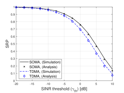
(a)

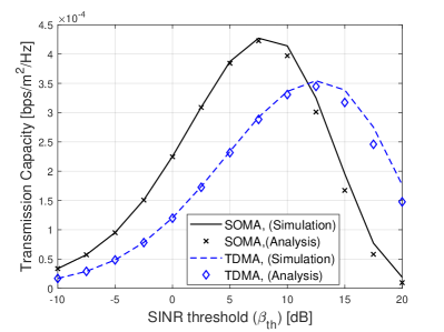
(b)

Figure 4: The SRP and the TC depending on SINR threshold where $\lambda^{\prime}_{\rm d}=0.00025$, $\lambda^{\prime}_{\rm r}=0.005$, $r_{0}=5$ m, $\phi=0.5$, $\tau=0.5$. In case 2, SOMA outperforms TDMA on both the SRP and the TC.

In this subsection, we compare SOMA and TDMA by SRP and TC depending on radius of guard zone and SINR threshold. In Fig. 3, we show SRP and TC of both SOMA and TDMA with $\lambda^{\prime}_{\rm d}$, $\lambda^{\prime}_{\rm r}$ and $\phi$, $\tau$ by case 1 in Section VIII-A. As we discuss in Proposition 2 and Proposition 3, TDMA outperforms SOMA in SRP while SOMA is superior to TDMA in the TC. We also observe that as radius of guard zone $r_{0}$ increases, SRP improves but TC degrades, which is matched to the analysis in Section VI-B and Section VII-B.

Fig. 4 shows SRP and TC with a system configuration in case 2 in Section VIII-B. It is observed that both SRP and TC could be better in SOMA if we consider case 2, which is mentioned in Remark 2. Note that in a general system parameter setting, we obtain SRP and the TC performance of case 1.

IX-B SRP and TC Dependence Power Splitting Factor and Time Division Factor

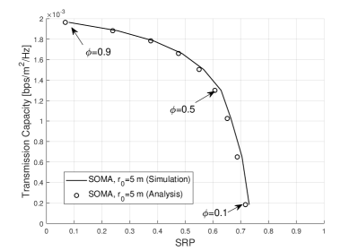
(a)

(b)

Figure 5: Change of SRP and TC as $\phi$ in SOMA and $\tau$ in TDMA increases where $\lambda^{\prime}_{\rm d}=0.01$, $\lambda^{\prime}_{\rm r}=0.1$, $\beta_{\rm th}=-5$ dB, $\gamma_{\rm th}=-10$ dB.

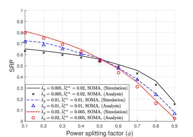
Figure 6: Change of SRP as $\phi$ increases with different ratio of the node density of the UAV-radar and the UAV-comm where $\gamma_{\rm th}=-10$ dB, which is analyzed in Propostion 1.

In this subsection, we evaluate SRP and TC depending on $\phi$ in SOMA and $\tau$ in TDMA. Fig. 5(a) shows that as $\phi$ increases TC improves but SRP decreases as we discuss in Section VI-C and in Section VII-C, which represents the impact of the different power ratio between the radar signal and the data signal on SRP and TC. In, Fig. 5(b), it is observed that TC increases as $\tau$ becomes large. On the other hand, the SRP slowly decreases as $\tau$ increases when we compare it with $\phi$ in SOMA in Fig. 5(a).

Fig. 6 show the effect of the different radio of the active UAV-radar node density $\bar{\lambda}_{\rm r}^{\rm s.o.}$ and the UAV-comm node density $\lambda_{\rm d}^{\prime}$ on the SRP in SOMA. It is observed that when $0.1<\phi<0.5$, higher UAV-comm node density achieves higher SRP while when $0.5<\phi<1$, higher active UAV-radar node density achieves higher SRP, which can be interpreted by Proposition 1.

IX-C SRP and TC Dependence Node Density of UAV-radar and UAV-comm

(a)

(b)

Figure 7: Change of SRP and TC depending on the UAV-radar node density where $\lambda^{\prime}_{\rm d}=0.01$, $r_{0}=5$ m, $\beta_{\rm th}=0$ dB, $\gamma_{\rm th}=-10$ dB, $\phi=0.5$, $\tau=0.5$.

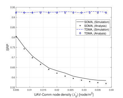
(a)

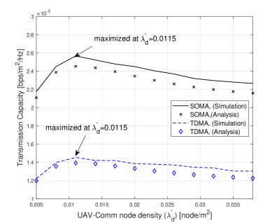
(b)

Figure 8: Change of SRP and TC depending on the UAV-comm node density where $\lambda^{\prime}_{\rm r}=0.01$, $r_{0}=5$ m, $\beta_{\rm th}=0$ dB, $\gamma_{\rm th}=-10$ dB, $\phi=0.5$, $\tau=0.5$.

In this subsection, we simulate the dependence of SRP and TC on the node density of the UAV-radar ($\lambda_{\rm r}^{\prime}$) and the UAV-comm ($\lambda_{\rm d}^{\prime}$). As we discuss in Section VI-A and Section VII-A, Fig. 7(a) shows that SRP is a decreasing function of $\lambda_{\rm r}^{\prime}$ for both SOMA and TDMA. In addition, in Fig. 7(b), it is observed that TC decreases as $\lambda_{\rm r}^{\prime}$ increases in SOMA, however, the TC is not affected by $\lambda_{\rm r}^{\prime}$ in TDMA.

In Fig. 8(a), we observe that SRP is a decreasing function of $\lambda_{\rm d}^{\prime}$ in SOMA, while SRP is not affected by $\lambda_{\rm r}^{\prime}$ in TDMA. Fig. 8 shows that TC is maximized at ${\lambda}_{\rm d}^{\prime\star}=0.0115$ for both SOMA and TDMA, which can be derived from Remark 1 and (7).

X Conclusion

In this paper, we investigate the coexistence of UAV radar and communication network. We deploy UAV-radars and UAV-comms by using HPPP where UAV-radars detect and track targets and UAV-comms communicate with their serving users in the same frequency band. We take into account two different multiple-access protocols, SOMA, and TDMA, to operate both radar signals and data signals simultanously. We analyze the performance of SRP in the radar detection scenario and TC in the data communication scenario. We show that in general, TDMA outperforms SOMA on SRP, while SOMA outperforms TDMA on TC. However, SOMA can achieve higher SRP as well as higher TC when the node density of UAV-radars is higher than that of UAV-comms (i.e., $\lambda_{\rm d}^{\prime}<\bar{\lambda}_{\rm r}$), for $\phi=\tau=0.5$, and $\mathsf{Pr}(\beta_{1}<\beta_{\rm th})<\frac{1}{2}$. We also find the UAV-comm node density that maximizes TC by derving the first and the second derivative of its analytic form and analyze the behavior of SRP and TC depending on the node density, the radius of the guard zone, the power splitting factor, and time division factor.

References

[1]
S. Hayat, E. Yanmaz, and R. Muzaffar, “Survey on Unmanned Aerial Vehicle
Networks for Civil Applications: A Communications Viewpoint,” IEEE
Commun. Surveys Tuts., vol. 18, no. 4, pp. 2624–2661, Apr. 2016.
[2]
A. Merwaday and I. Guvenc, “UAV Assisted Heterogeneous Networks for Public
Safety Communications,” in Proc. IEEE Wireless Commun. Netw. Conf. (WCNC), New Orleans, LA, USA, Mar. 2015, pp. 329–334.
[3]
P. Chandhar, D. Danev, and E. G. Larsson, “Massive MIMO for Communications
With Drone Swarms,” IEEE Trans. Wireless Commun., vol. 17, no. 3,
pp. 1604–1629, Mar. 2018.
[4]
S. Ortiz, C. T. Calafate, J.-C. Cano, P. Manzoni, and C. K. Toh, “A UAV-Based
Content Delivery Architecture for Rural Areas and Future Smart Cities,”
IEEE Internet Computing, vol. 23, no. 1, pp. 29–36, Jan. 2019.
[5]
L. Zheng, M. Lops, Y. C. Eldar, and X. Wang, “Radar and Communication
Coexistence: An Overview: A Review of Recent Methods,” IEEE Sig.
Proc. Mag., vol. 36, no. 5, pp. 85–99, Sep. 2019.
[6]
H. ElSawy, A. Sultan-Salem, M.-S. Alouini, and M. Z. Win, “Modeling and
Analysis of Cellular Networks Using Stochastic Geometry: A Tutorial,”
IEEE Commun. Surveys Tuts., vol. 19, no. 1, pp. 167–203, 2017.
[7]
A. M. Hunter, J. G. Andrews, and S. Weber, “Transmission Capacity of Ad Hoc
Networks with Spatial Diversity,” IEEE Trans. Wireless Commun.,
vol. 7, no. 12, pp. 5058–5071, Dec. 2008.
[8]
J. Park, B. Clerckx, C. Song, and Y. Wu, “An Analysis of the Optimum Node
Density for Simultaneous Wireless Information and Power Transfer in Ad Hoc
Networks,” IEEE Trans. Veh. Technol., vol. 67, no. 3, pp.
2713–2726, Mar. 2018.
[9]
J. Park, J.-P. Hong, W. Shin, and S. Kim, “Performance Analysis of
Distributed Antenna System for Downlink Ultrareliable Low-Latency
Communications,” IEEE Syst. J., vol. 15, no. 1, pp. 518–525, Mar.
2021.
[10]
A. Al-Hourani, R. J. Evans, S. Kandeepan, B. Moran, and H. Eltom, “Stochastic
Geometry Methods for Modeling Automotive Radar Interference,” IEEE
Trans. Intell. Transp. Syst., vol. 19, no. 2, pp. 333–344, Feb. 2018.
[11]
Z. Fang, Z. Wei, X. Chen, H. Wu, and Z. Feng, “Stochastic Geometry for
Automotive Radar Interference With RCS Characteristics,” IEEE
Wireless Commun. Lett., vol. 9, no. 11, pp. 1817–1820, Nov. 2020.
[12]
A. Munari, L. Simić, and M. Petrova, “Stochastic Geometry Interference
Analysis of Radar Network Performance,” IEEE Commun. Lett.,
vol. 22, no. 11, pp. 2362–2365, Nov. 2018.
[13]
M. Rebato, J. Park, P. Popovski, E. De Carvalho, and M. Zorzi, “Stochastic
Geometric Coverage Analysis in mmWave Cellular Networks With Realistic
Channel and Antenna Radiation Models,” IEEE Trans. Commun.,
vol. 67, no. 5, pp. 3736–3752, May 2019.
[14]
X. Yu, J. Zhang, M. Haenggi, and K. B. Letaief, “Coverage Analysis for
Millimeter Wave Networks: The Impact of Directional Antenna Arrays,”
IEEE J. Sel. Areas Commun., vol. 35, no. 7, pp. 1498–1512, July
2017.
[15]
C. Wang and H.-M. Wang, “Physical Layer Security in Millimeter Wave Cellular
Networks,” IEEE Trans. Wireless Commun., vol. 15, no. 8, pp.
5569–5585, Aug. 2016.
[16]
M. M. Azari, G. Geraci, A. Garcia-Rodriguez, and S. Pollin, “UAV-to-UAV
Communications in Cellular Networks,” IEEE Trans. Wireless
Commun., vol. 19, no. 9, pp. 6130–6144, Sep. 2020.
[17]
C.-H. Liu, K.-H. Ho, and J.-Y. Wu, “MmWave UAV Networks With Multi-Cell
Association: Performance Limit and Optimization,” IEEE J. Sel.
Areas Commun., vol. 37, no. 12, pp. 2814–2831, Dec. 2019.
[18]
V. V. Chetlur and H. S. Dhillon, “Downlink Coverage Analysis for a Finite 3-D
Wireless Network of Unmanned Aerial Vehicles,” IEEE Trans. Commun., vol. 65, no. 10, pp. 4543–4558, Oct. 2017.
[19]
W. Yi, Y. Liu, Y. Deng, and A. Nallanathan, “Clustered UAV Networks With
Millimeter Wave Communications: A Stochastic Geometry View,” IEEE
Trans. Commun., vol. 68, no. 7, pp. 4342–4357, July 2020.
[20]
X. Wang and M. C. Gursoy, “Coverage Analysis for Energy-Harvesting
UAV-Assisted mmWave Cellular Networks,” IEEE J. Sel. Areas
Commun., vol. 37, no. 12, pp. 2832–2850, Dec. 2019.
[21]
W. Yi, Y. Liu, E. Bodanese, A. Nallanathan, and G. K. Karagiannidis, “A
Unified Spatial Framework for UAV-Aided MmWave Networks,” IEEE
Trans. Commun., vol. 67, no. 12, pp. 8801–8817, Dec. 2019.
[22]
M. Gapeyenko, D. Moltchanov, S. Andreev, and R. W. Heath, “Line-of-Sight
Probability for mmWave-Based UAV Communications in 3D Urban Grid
Deployments,” IEEE Trans. Wireless Commun., vol. 20, no. 10, pp.
6566–6579, Oct. 2021.
[23]
Z. Huang, C. Chen, and M. Pan, “Multiobjective UAV Path Planning for
Emergency Information Collection and Transmission,” IEEE Internet
Things J., vol. 7, no. 8, pp. 6993–7009, Aug. 2020.
[24]
X. Sun, W. Yang, and Y. Cai, “Secure Communication in NOMA-Assisted
Millimeter-Wave SWIPT UAV Networks,” IEEE Internet Things J.,
vol. 7, no. 3, pp. 1884–1897, Mar. 2020.
[25]
M. M. U. Chowdhury, S. J. Maeng, E. Bulut, and I. Guvenc, “3-D Trajectory
Optimization in UAV-Assisted Cellular Networks Considering Antenna Radiation
Pattern and Backhaul Constraint,” IEEE Trans. Aerosp. Electron.
Syst., vol. 56, no. 5, pp. 3735–3750, Oct. 2020.
[26]
Y. Pan, K. Wang, C. Pan, H. Zhu, and J. Wang, “UAV-Assisted and Intelligent
Reflecting Surfaces-Supported Terahertz Communications,” IEEE
Wireless Commun. Lett., vol. 10, no. 6, pp. 1256–1260, June 2021.
[27]
M. Cui, G. Zhang, Q. Wu, and D. W. K. Ng, “Robust Trajectory and Transmit
Power Design for Secure UAV Communications,” IEEE Trans. Veh. Technol., vol. 67, no. 9, pp. 9042–9046, Sep. 2018.
[28]
S. J. Maeng, Y. Yapici, I. Guvenc, H. Dai, and A. Bhuyan, “Precoder Design
for mmWave UAV Communications with Physical Layer Security,” in
Proc. IEEE Int. Workshop Signal Process. Adv. Wireless Commun. (SPAWC), Atlanta, GA, USA, May 2020, pp. 1–5.
[29]
R. O. R. Jenssen, M. Eckerstorfer, and S. Jacobsen, “Drone-Mounted
Ultrawideband Radar for Retrieval of Snowpack Properties,” IEEE
Trans. Instrum. Meas., vol. 69, no. 1, pp. 221–230, Jan. 2020.
[30]
S. Z. Gurbuz, U. Kaynak, B. Ozkan, O. C. Kocaman, F. Kiyici, and B. Tekeli,
“Design Study of a Short-range Airborne UAV Radar for Human Monitoring,”
in Proc. IEEE Asilomar Conf. on Signals, Syst., and Comput.,
Pacific Grove, CA, USA, Nov. 2014, pp. 568–572.
[31]
G. Fasano, A. Renga, A. R. Vetrella, G. Ludeno, I. Catapano, and F. Soldovieri,
“Proof of Concept of Micro-UAV-based Radar Imaging,” in Proc.
International Conference on Unmanned Aircraft Systems (ICUAS), Miami, FL,
USA, June 2017, pp. 1316–1323.
[32]
E. Vinogradov, D. A. Kovalev, and S. Pollin, “Simulation and Detection
Performance Evaluation of a UAV-mounted Passive Radar,” in Proc. IEEE Int. Symp. Personal, Indoor, Mobile Radio Commun. (PIMRC), Bologna,
Italy, Sep. 2018, pp. 1185–1191.
[33]
F. Liu, C. Masouros, A. Li, and T. Ratnarajah, “Robust MIMO Beamforming for
Cellular and Radar Coexistence,” IEEE Wireless Commun. Lett.,
vol. 6, no. 3, pp. 374–377, June 2017.
[34]
J. Qian, M. Lops, L. Zheng, and X. Wang, “Joint Design for Co-existence of
MIMO Radar and MIMO Communication System,” in Proc. IEEE Asilomar
Conf. on Signals, Syst., and Comput., Pacific Grove, CA, USA, Oct. 2017,
pp. 568–572.
[35]
Q. Wu, J. Xu, Y. Zeng, D. W. K. Ng, N. Al-Dhahir, R. Schober, and A. L.
Swindlehurst, “A Comprehensive Overview on 5G-and-Beyond Networks With
UAVs: From Communications to Sensing and Intelligence,” IEEE J.
Sel. Areas Commun., vol. 39, no. 10, pp. 2912–2945, Oct. 2021.
[36]
X. Chen, Z. Feng, Z. Wei, F. Gao, and X. Yuan, “Performance of Joint
Sensing-Communication Cooperative Sensing UAV Network,” IEEE
Trans. Veh. Technol., vol. 69, no. 12, pp. 15 545–15 556, Dec. 2020.
[37]
A. Al-Hourani, S. Kandeepan, and S. Lardner, “Optimal LAP Altitude for
Maximum Coverage,” IEEE Wireless Commun. Lett., vol. 3, no. 6, pp.
569–572, Dec. 2014.
[38]
M. Haenggi, “Mean Interference in Hard-Core Wireless Networks,”
IEEE Commun. Lett., vol. 15, no. 8, pp. 792–794, Aug. 2011.