Top-Down Synthesis for Library Learning

Abstract.

This paper introduces corpus-guided top-down synthesis as a mechanism for synthesizing library functions that capture common functionality from a corpus of programs in a domain specific language (DSL). The algorithm builds abstractions directly from initial DSL primitives, using syntactic pattern matching of intermediate abstractions to intelligently prune the search space and guide the algorithm towards abstractions that maximally capture shared structures in the corpus. We present an implementation of the approach in a tool called Stitch and evaluate it against the state-of-the-art deductive library learning algorithm from DreamCoder. Our evaluation shows that Stitch is 3-4 orders of magnitude faster and uses 2 orders of magnitude less memory while maintaining comparable or better library quality (as measured by compressivity). We also demonstrate Stitch’s scalability on corpora containing hundreds of complex programs that are intractable with prior deductive approaches and show empirically that it is robust to terminating the search procedure early—further allowing it to scale to challenging datasets by means of early stopping.

1. Introduction

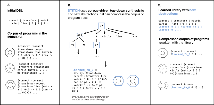
Figure 1. (A) Given an initial DSL of lower-level primitives and a corpus of programs written in the initial DSL, (B) Stitch uses a fast and memory efficient corpus-guided top-down search algorithm to construct function abstractions which maximally capture shared structure across the corpus of programs. (C) Stitch automatically rewrites the initial corpus using the learned library functions.

One way programmers manage complexity is by hiding functionality behind functional abstractions. For example, consider the graphics programs at the bottom of Fig. 1A. Each uses a generic set of drawing primitives and renders a technical schematic of a hardware component, shown to the left of each program. Faced with the task of writing more of these rendering programs, an experienced human programmer likely would not continue using these low-level primitives. Instead, they would introduce new functional abstractions, like the one at the bottom of Fig. 1B which renders a regular polygon given a size and number of sides. Useful abstractions like these allow more concise and legible programs to render the existing schematics. More importantly, well-written abstractions should generalize, making it easier to write new graphics programs for similar graphics tasks.

Recently, the program synthesis community has introduced new approaches that can mimic this process, automatically building a library of functional abstractions in order to tackle more complex synthesis problems (Ellis et al., 2021, 2020; Shin et al., 2019; Lázaro-Gredilla et al., 2019; Dechter et al., 2013). One popular approach to library learning is to search for common tree fragments across a corpus of programs, which can be introduced as new abstractions (Shin et al., 2019; Lázaro-Gredilla et al., 2019; Dechter et al., 2013). Ellis et al. 2021, however, introduces an algorithm that reasons about variable bindings to abstract out well-formed functions instead of just tree fragments. While it produces impressive results, the system in Ellis et al. 2021 takes a deductive approach to library learning that is difficult to scale to larger datasets of longer and deeper input programs. This approach is deductive in that it uses semantics-preserving rewrite rules to attempt to refactor existing programs to expose shared structure. This requires representing and evaluating an exponentially large space of proposed refactorings to identify common functionality across the corpus. Prior work, such as Ellis et al. 2021, 2020, approaches this challenge by combining a dynamic bottom-up approach to refactoring with version spaces to more efficiently search over the refactored programs. However, these deductive approaches face daunting memory and search requirements as the corpus scales in size and complexity.

This paper introduces an alternate approach to library learning, while preserving the focus on well-formed function abstractions from Ellis et al. 2021. Instead of taking a deductive approach based on refactoring the corpus with rewrite rules, we directly synthesize abstractions. We call this approach corpus-guided top-down synthesis, and it is based on the insight that when applied to the task of synthesizing abstractions, top-down search can be guided precisely towards discovering shared abstractions over a set of existing training programs. At every step of the search, syntactic comparisons between a partially constructed abstraction and the set of training programs can be used to strongly constrain the search space and direct the search towards abstractions that capture the greatest degree of shared syntactic structure.

We implement this approach in Stitch, a corpus-guided top-down library learning tool written in Rust (Fig. 1). Stitch is open-source and available both as a Python package and a Rust crate; the code, installation instructions, and tutorials are available at the GitHub. We evaluate Stitch through a series of experiments (Section 6), and find that: Stitch learns libraries of comparable quality to those found by the algorithm of Ellis et al. 2021 on their iterative bootstrapped library learning task, while being 3-4 orders of magnitude faster and using 2 orders of magnitude less memory (Section 6.1); Stitch learns high quality libraries within seconds to single-digit minutes when run on corpora containing a few hundred programs with mean lengths between 76–189 symbols (sourced from Wong et al. 2022), while even the simplest of these corpora lies beyond the reach of the algorithm of Ellis et al. 2021 (Section 6.2); and that Stitch degrades gracefully when resources are constrained (Section 6.3). We also perform ablation studies to expose the relative impact of different optimizations in Stitch (Section 6.4). Finally, we show that Stitch is complementary to deductive rewrite approaches (Section 6.5).

In summary, our paper makes the following contributions:

1. Corpus-guided top-down synthesis (CTS): A novel, strongly-guided branch-and-bound algorithm for synthesizing function abstractions (Sec. 3).

2. CTS for program compression: An instantiation of the CTS framework for utility functions favoring abstractions that compress a corpus of programs (Sec. 4).

3. Stitch: A parallel Rust implementation of CTS for compression that achieves 3-4 orders of magnitude of speed and memory improvements over prior work, and the analysis of its performance, scaling, and optimizations through several experiments (Sec. 6).

2. Overview

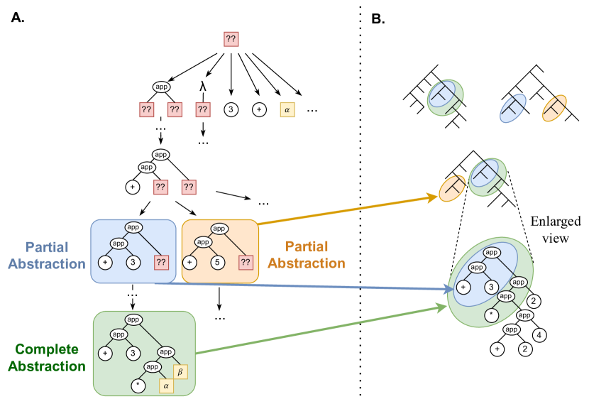
Figure 2. (A) Schematic of corpus-guided top-down search (CTS). Partial abstractions can contain holes indicating unfinished subtrees, denoted ??, while complete abstractions do not contain holes. (B) Partial and complete abstractions match at locations in the corpus. The blue partial abstraction can be expanded into the green complete abstraction so the green abstraction matches in a subset of places that the blue abstraction does. For complete abstractions, matching indicates that the subtree can be rewritten to use the abstraction.

In this section, we build intuition for the algorithmic insights that power Stitch. As a running example, we focus on learning a single abstraction from the following corpus of programs:

(1) $$\lambda x.\ \texttt{{\color[rgb]{0,0,1}+ 3} ({\color[rgb]{0,0,1}*} (+ 2 4) 2)}$$

$$\lambda xs.\ \texttt{map ($\lambda x.\ ${\color[rgb]{0,0,1}+ 3} ({\color[rgb]{0,0,1}*} 4 (+ 3 x))) xs}$$

$$\lambda x.\ \texttt{* 2 ({\color[rgb]{0,0,1}+ 3} ({\color[rgb]{0,0,1}*} x (+ 2 1)))}$$

The notion of what a good abstraction is depends on the application, so our algorithm is generic over the utility function that we seek to maximize. Following prior work (Ellis et al., 2021; Shin et al., 2019; Dechter et al., 2013) we focus on compression as a utility function: a good abstraction is one which minimizes the size of the corpus when rewritten with the abstraction. The utility function used by Stitch is detailed in Section 4 and corresponds exactly to the compression objective, but at a high level the function seeks to maximize the product of the size of the abstraction and the number of locations where the abstraction can be used. This product balances two key features of a highly compressive abstraction: the abstraction should be general enough that it applies in many locations, but specific enough that it captures a lot of structure at each location.

The optimal abstraction that maximizes our utility in this example is:

(2) $$\texttt{{\color[rgb]{0,0,1}fn0}}=\lambda\alpha.\ \lambda\beta.\texttt{(+ 3 (* $\alpha$ $\beta$))}$$

And the shared structure that this abstraction captures is highlighted in blue in Eq. 1. When rewritten to use this abstraction, the size of the resulting programs is minimized:

(3) $$\lambda x.\ \texttt{{\color[rgb]{0,0,1}fn0} (+ 2 4) 2}$$

$$\lambda xs.\ \texttt{map ($\lambda x.\ ${\color[rgb]{0,0,1}fn0} 4 (+ 3 x)) xs}$$

$$\lambda x.\ \texttt{* 2 ({\color[rgb]{0,0,1}fn0} x (+ 2 1))}$$

Stitch synthesizes the optimal abstraction directly through top-down search. Top-down search methods construct program syntax trees by iteratively refining partially-completed programs that have unfinished holes, until a complete program that meets the specification is produced (Feser et al., 2015; Polikarpova et al., 2016; Balog et al., 2016; Ellis et al., 2021; Nye et al., 2021; Shah et al., 2020). This kind of search is often made efficient by identifying branches of the search tree that can be pruned away because the algorithm can efficiently determine that none of the programs in that branch can be correct. We aim to apply a similar idea to the problem of synthesizing good abstractions; the idea is to explore the space of functions in the same top-down way, but in search of a function that maximizes the utility measure. The key observation is that this new objective affords even more aggressive pruning opportunities than the traditional correctness objective, allowing us to synthesize optimal abstractions very efficiently. We call this approach corpus-guided top-down search (CTS).

Corpus-Guided Top-Down Search.

Like other top-down synthesis approaches, our algorithm explores the space of abstractions by repeatedly refining abstractions with holes, as illustrated in Fig. 2A. We call abstractions with holes partial abstractions in contrast to complete abstractions which have no holes. Our top-down algorithm searches over abstraction bodies, so to synthesize the optimal abstraction fn0 in our running example, we synthesize its body: (+ 3 (* $\alpha$ $\beta$)).

We say that a partial abstraction matches at a subtree in the corpus if there’s a possible assignment to the holes and arguments that yields the subtree. For example, consider the subtree (+ 3 (* (+ 2 4) 2) from the first program in our running example, shown as a syntax tree at the bottom of figure 2B. The partial abstraction (+ 3 ??) shown in blue matches here with the hole $\texttt{??}=\texttt{(* (+ 2 4) 2)}$, and the complete abstraction (+ 3 (* $\alpha$ $\beta$)) matches here with $\alpha=\texttt{(+ 2 4)}$ and $\beta=\texttt{2}$. For complete abstractions, matching corresponds to being able to use the abstraction to rewrite this subtree, resulting in compression. We refer to the set of subtrees at which a complete or partial abstraction matches as the set of match locations. For example, the three match locations of (+ 3 (* $\alpha$ $\beta$)) are the subtree (+ 3 (* (+ 2 4) 2)) in the first program, (+ 3 (* 4 (+ 3 x))) in the second program, and (+ 3 (* x (+ 2 1))) in the third program.

In traditional top-down synthesis, a branch of search can be safely pruned by proving that a program satisfying the specification cannot exist in that branch. In CTS, we can safely prune a branch of search if we can prove that it cannot contain the optimal abstraction. One way to prove this is by computing an upper bound on the utility of abstractions in the branch, and discarding the branch if we have previously found an abstraction with a utility that is higher than this bound. An efficient and conservative way to compute this upper bound is to overapproximate the set of match locations, then upper bound the compressive utility gain from each match location.

Our key observation to compute this bound is that during search, expanding a hole in a partial abstraction yields an abstraction that is more precise and thus matches at a subset of the locations that the original matched at. This subset observation is depicted in Fig. 2 where the refinement of the partial abstraction (+ 3 ??) (blue) to the goal (+ 3 (* $\alpha$ $\beta$)) (green) results in a larger abstraction that matches at a subset of the locations (match locations shown at the top of Fig. 2B). An important consequence of this is that the match locations of a partial abstraction serves as an over-approximation of the match locations of any abstraction in this branch of top-down search.

To upper bound the compressive utility gained by rewriting at a match location, notice that the most compressive abstraction that matches at a subtree is the constant abstraction corresponding to the subtree itself. For example, the largest possible abstraction at (+ 3 (* (+ 2 4) 2) is just (+ 3 (* (+ 2 4) 2). In other words, the size of the subtree is a strict upper bound on how much compression can be achieved at a match location. Thus we get the upper bound for some partial abstraction $A_{\texttt{??}}$:

(4) $$U_{\text{upperbound}}(A_{\texttt{??}})=\sum_{e\in\text{matches}(A_{\texttt{??}})}{\text{size}(e)}$$

Equipped with this bound, our algorithm performs a branch-and-bound style top-down search, where at each step of search it discards all partial abstractions that have utility upper bounds that are less than the utility of the best complete abstraction found so far.

Our full algorithm presented in Section 3 has some additional complexity. It handles rewriting in the presence of variables soundly, it uses an exact utility function that accounts for additional compression gained by using the same variable in multiple places, and it handles situations where match locations overlap and preclude one another. We also introduce two other important forms of pruning while maintaining the optimality of the algorithm, and we use the upper bound as a heuristic to prioritize more promising branches of search first.

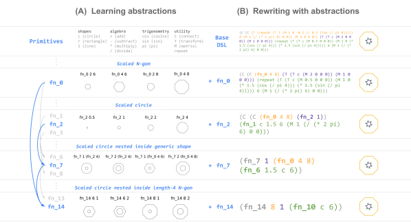
Figure 3. Visualization of Stitch library learning on the nuts-bolts subdomain from Wong et al. 2022. (A) From the base DSL primitives (top row), Stitch iteratively discovers a series of abstractions that compress programs in the domain. Arrows demonstrate how abstractions from selected iterations build on one another to achieve increasingly higher-level behaviors. (B) Rewriting a single item from the domain with the cumulative benefit of discovered abstractions yields increasingly compact expressions. Colors indicate correspondence between object parts and program fragments: orange = outer octagon, green = ring of six circles, purple = inner circle.

Building Up Abstraction Libraries.

The top-down search algorithm described above yields a single abstraction. However, we can easily run this algorithm for multiple iterations on a corpus of programs to build up an entire library of abstractions. Fig. 3 illustrates the power of this kind of iterative library learning, which interleaves compression and rewriting. At each iteration, Stitch discovers a single abstraction that is used to rewrite the entire corpus of programs. Successive iterations therefore yield abstractions that build hierarchically on one another, achieving increasingly higher-level behaviors. As the library grows to contain richer and more complex abstractions, individual programs shrink into compact expressions.

Structure of the Paper.

In the subsequent sections, we formalize our corpus-guided top-down search algorithm (Section 3), its application to the problem of compression (Section 4), and how it may be layered on top of data structures such as version spaces (Section 5). We then report experimental results (Section 6) showcasing both diverse library learning settings as well as ablations of Stitch’s search mechanisms. Finally, we conclude by situating Stitch within the landscape of related work (Section 7) and future work (Section 8) in the areas of library learning and program synthesis.

3. Corpus-Guided Top-Down Search

3.1. Problem Setup

In this section we provide the definitions necessary to understand our problem.

Grammar

Our algorithm operates on lambda-calculus expressions with variables represented through de Bruijn indices (de Bruijn, 1972); expressions come from a context-free grammar of the form $e\Coloneqq\lambda.\ e^{\prime}\mid e^{\prime}\ e^{\prime\prime}\mid\$i\mid t$, where $t\in\mathcal{G}_{\texttt{sym}}$ refers to the set of built-in primitives in the domain-specific language. For example, in an arithmetic domain $\mathcal{G}_{\texttt{sym}}$ would include operators like + and constants like 3. We say that $e^{\prime}$ is a subexpression of $e$ if $e=C[e^{\prime}]$, where $C$ is a context as defined in the contextual semantics of Felleisen and Hieb 1992. An expression is closed if it has no free variables, in which case the expression is also a program. A set of programs $\mathcal{P}$ is a corpus.

When representing variables through de Bruijn indices, $\$i$ refers to the variable bound by the $i$th closest lambda above it. Thus $\lambda x.\ \lambda y.\ (x\ y)$ is represented as $\lambda.\ \lambda.\ (\$1\ \$0)$. Beta reduction with de Bruijn indices requires upshifting: incrementing free variables in the argument when substitution recurses into a lambda, since the free variables must now point past one more lambda. Similarly, inverse beta reduction requires downshifting.

Abstraction

Given a grammar $\mathcal{G}$, we define the abstraction grammar $\mathcal{G}_{A}$ as $\mathcal{G}$ extended to include abstraction variables, denoted by Greek letters $\alpha$, $\beta$, etc. Formally, $A\Coloneqq\lambda.\ A^{\prime}\mid A^{\prime}\ A^{\prime\prime}\mid\$i\mid t\mid\alpha$ where $t\in\mathcal{G}_{\texttt{sym}}$. A term $A$ from this grammar represents the body of an abstraction; e.g. the abstraction $\lambda\alpha.\ \lambda\beta.\ (\texttt{+}\ \alpha\ \beta)$ is simply represented by the term $(\texttt{+}\ \alpha\ \beta)$ from the language of $\mathcal{G}_{A}$.

Partial Abstraction

A partial abstraction $A_{\texttt{??}}$ is an abstraction that can additionally include holes. A hole, denoted by ??, represents an unfinished subtree of the abstraction. Thus, $A_{\texttt{??}}\Coloneqq A\mid\texttt{??}\mid\lambda.\ A_{\texttt{??}}^{\prime}\mid A_{\texttt{??}}^{\prime}\ A_{\texttt{??}}^{\prime\prime}$. Any abstraction is thus also a partial abstraction. Given a grammar $\mathcal{G}$, the grammar of partial abstractions is denoted by $\mathcal{G}_{A_{\texttt{??}}}$. Each hole in a partial abstraction $A$ can be referred to by a unique index, which can be explicitly written as $\texttt{??}_{i}$.

Lambda-Aware Unification

We introduce lambda-aware unification as a modification of traditional unification adapted to our algorithm. $\textsc{LambdaUnify}(A,e)$ returns a mapping (if one exists) from abstraction variables and holes to expressions $[\alpha_{i}\to e_{i}^{\prime},\ \ldots,\ \texttt{??}_{j}\to u_{j}^{\prime},\ \ldots]$ such that

(5) $$(\lambda\alpha_{i}.\ \ldots\ \lambda\texttt{??}_{j}.\ \ldots A)\ e_{i}^{\prime}\ \ldots\ u_{j}^{\prime}\ \ldots=e$$

through beta reduction. A key difference from traditional unification is that the expression $e$ may be deep inside a program written using de Bruijn indices, so LambdaUnify must perform some index arithmetic in order to generate its output mapping; in particular, raising a subtree out of a lambda during this inverse beta reduction requires downshifting variables in it.

The definition of LambdaUnify is presented in Fig. 4 (left). In U-App, $\textsc{merge}(l_{1},l_{2})$ merges two $[\alpha_{i}\to e_{i}]$ mappings to create a new mapping that includes all bindings from $l_{1}$ and $l_{2}$, and fails if the same abstraction variable $\alpha$ maps to different expressions in $l_{1}$ and $l_{2}$. The rule U-Same applies only when the abstraction argument to LambdaUnify is an expression (i.e. it contains no holes or abstraction variables) and is syntactically identical to the expression it is being unified with. In U-Lam, DownshiftAll returns a new mapping with all abstracted expressions $e$ and hole expressions $u$ downshifted using the $\downarrow$ operator presented in Fig. 4 (right). The $\downarrow$ operator has been modified from traditional downshifting to allow for partial abstractions that contain holes $\texttt{??}_{j}$ to break the rules of variable binding, because holes represent unfinished subtrees of the abstraction.

In particular, a new syntactic form ”$\&i$” is used to represent a $\$i$ variable that has been downshifted further than traditional downshifting would permit. $\&i$ variables are created by $\downarrow$ when a traditional downshift would otherwise convert a free variable to a (different, incorrect) bound variable. These variables represent references to lambdas present within the body of the abstraction and are allowed in expressions $u_{j}^{\prime}$ bound to holes but not expressions $e_{i}^{\prime}$ bound to abstraction variables.

To account for $\&i$ variables, the beta reduction used in Eq. 5, which is defined in Fig. 5, uses a modified upshift operator $\uparrow$ defined to be an inverse to the $\downarrow$ operator. With this modification of beta reduction, any $\&i$ variables with negative indices will ultimately be shifted back to positive indices during reduction. Furthermore, the beta reduction procedure is equivalent to traditional beta reduction when there are no holes and thus no $\&i$ variables.

*[left=U-AbsVar] LambdaUnify(α, e) ↝[ α→e ] *[left=U-Hole] LambdaUnify(??_i, e) ↝[ ??_i →e ] *[left=U-App] LambdaUnify(A_1,e_1) ↝l_1
LambdaUnify(A_2,e_2) ↝l_2
l = merge(l_1,l_2) LambdaUnify((A_1 A_2),(e_1 e_2)) ↝l *[left=U-Lam] LambdaUnify(A, e) ↝l’
l = DownshiftAll(l’) LambdaUnify((λ. A),(λ. e)) ↝l *[left=U-Same] LambdaUnify(e,e) ↝[ ]

$$\textsc{DownshiftAll}([\alpha_{i}\to e_{i}^{\prime},\ \texttt{??}_{j}\to u_{j}^{\prime},\ ...])$$

$$\ \ \ \ =[\alpha_{i}\to\ \downarrow_{0}e_{i}^{\prime},\ \texttt{??}_{j}\to\ \downarrow_{0}u_{j}^{\prime},\ ...]$$

$$\downarrow_{d}\lambda.b=\lambda.\downarrow_{d+1}b$$

$$\downarrow_{d}(fx)=(\downarrow_{d}f\ \downarrow_{d}x)$$

$$\downarrow_{d}\$i=\begin{cases}\$i,&\text{if }i<d\\ \$(i-1),&\text{if }i>d\\ \&(i-1),&\text{if }i=d\\ \end{cases}$$

$$\downarrow_{d}\&i=\&(i-1),$$

$$\downarrow_{d}t=t,\ \text{if $t$ is a primitive (i.e. $t\in\mathcal{G}_{\texttt{sym}}$) }$$

Figure 4. (Left) Inference rules for lambda-aware unification. (Right) Definition of DownshiftAll.

$$(\lambda\alpha_{i}.\ \ldots\ \lambda\texttt{??}_{j}.\ \ldots A)\ e_{i}^{\prime}\ \ldots\ u_{j}^{\prime}\ \ldots$$

$$\ \ \ \ =[\alpha_{i}\to e_{i}^{\prime},\ \texttt{??}_{j}\to u_{j}^{\prime},\ ...]\circ A$$

$$l\circ\lambda.b=\lambda.\textsc{UpshiftAll}(l)\circ b$$

$$l\circ(fx)=(l\circ f)(l\circ x)$$

$$l\circ\$i=\$i$$

$$l\circ\alpha_{i}=l[\alpha_{i}]$$

$$l\circ\texttt{??}_{i}=l[\texttt{??}_{i}]$$

$$l\circ t=t,\ \text{for $t\in\mathcal{G}_{\texttt{sym}}$}$$

$$\textsc{UpshiftAll}([\alpha_{i}\to e_{i}^{\prime},\ \texttt{??}_{j}\to u_{j}^{\prime},\ ...])$$

$$\ \ \ \ =[\alpha_{i}\to\ \uparrow_{0}e_{i}^{\prime},\ \texttt{??}_{j}\to\ \uparrow_{0}u_{j}^{\prime},\ ...]$$

$$\uparrow_{d}\lambda.b=\lambda.\uparrow_{d+1}b$$

$$\uparrow_{d}(fx)=(\uparrow_{d}f\ \uparrow_{d}x)$$

$$\uparrow_{d}\$i=\begin{cases}\$i,&\text{if }i<d\\ \$(i+1),&\text{if }i\geq d\\ \end{cases}$$

$$\uparrow\&i=\begin{cases}\&(i+1),&\text{if }i+1\neq d\\ \$(i+1),&\text{if }i+1=d\\ \end{cases}$$

$$\uparrow_{d}t=t,\ \text{for $t\in\mathcal{G}_{\texttt{sym}}$}$$

Figure 5. (Left) Definition of modified beta reduction and substitution ($\circ$). (Right) Definition of UpshiftAll.

We provide a proof of the correctness of LambdaUnify with respect to Eq. 5 in Appendix B, as well as a Coq proof of the correctness in stitch.v in the supplemental material. However, to understand the key idea behind the proof we focus here on an example illustrating the different cases involving the $\downarrow$ operator and $\&i$ indices. Consider what happens when you run

(6) $$\textsc{LambdaUnify}(\lambda.\ f\ \texttt{??}_{0},\ \lambda.\ e)$$

By Eq. 5, the goal is to produce a mapping $[\texttt{??}_{0}\rightarrow u^{\prime}_{0}]$ such than when replacing $\texttt{??}_{0}$ with $u^{\prime}_{0}$ it produces $(\lambda.\ e)$. In other words, $(\lambda.\ \lambda.\ f\ \$1)\ u^{\prime}_{0}=\lambda.\ e$. Now, suppose

(7) $$\textsc{LambdaUnify}(f~{}\texttt{??}_{0},\ e)\rightsquigarrow[\texttt{??}_{0}\rightarrow\lambda.\ \$i]$$

This means that $(\lambda.\ f\ \$0)\ (\lambda.\ \$i)=e$ so $e=f\ (\lambda.\ \$i)$. There are three possibilities for $i$ that need to be considered, corresponding to the 3 cases in the definition of $\downarrow_{d}\$i$. In the first case, when $i=0$ and thus $e=f\ (\lambda.\ \$0)$, it means that $\$i$ in Eq. 7 is bound to the lambda in the return mapping. In this case, DownshiftAll in U-Lam should not do anything because if we can replace $\texttt{??}_{0}$ with $(\lambda.\ \$0)$ in $(f\ \texttt{??}_{0})$ to produce $e$, the same replacement in $(\lambda.\ f\ \texttt{??}_{0})$ will produce $(\lambda.\ e)$.

The second case is when $i\geq 2$; this means that $e$ has some variables that were defined outside of it and they have been captured by $\texttt{??}_{0}$. For example, if $i=2$ and thus $e=f\ (\lambda.\ \$2)$, the solution to Eq. 6 is $[\texttt{??}_{0}\rightarrow\lambda.\ \$1]$, since $(\lambda.\ \lambda.\ f\ \$1)(\lambda.\ \$1)=\lambda.\ e$; in other words, when computing $\textsc{LambdaUnify}(\lambda.~{}f~{}\texttt{??}_{0},\ \lambda.\ e)$ from Eq. 7, the $\$i$ in the return mapping has to be downshifted to account for the fact that it will be substituted inside an additional lambda.

The third case, when $i=1$, is more problematic. In this case, we have that $e=f\ (\lambda.\ \$1)$. This creates a problem, since there is no $i$ such that $(\lambda.\ \lambda.\ f\ \$1)(\lambda.\ \$i)=\lambda.\ e$; the $\$i$ needs to refer to the lambda surrounding $e$. The downshift operator addresses this through the special treatment of the $\&i$ index.

LambdaUnify relates to prior work on unification modulo binders (Huet, 1975; Miller, 1991, 1992; Dowek et al., 1995, 1996) but focuses on a more efficiently solvable syntax-driven subset of the more general unification problems tackled in this prior work. We give a more detailed comparison to this prior work in Section 7.

Match Locations

The set of match locations of a partial abstraction $A_{\texttt{??}}$ in a corpus $\mathcal{P}$, denoted $\textsc{Matches}(\mathcal{P},A_{\texttt{??}})$, is the maximal set of context-expression pairs $\{(C_{1},e_{1}),(C_{2},e_{2}),\ \ldots,(C_{k},e_{k})\}$ such that $\forall k.\ p=C_{k}[e_{k}]$ and $p\in\mathcal{P}$ and $\textsc{LambdaUnify}(e_{k},A_{\texttt{??}})$ succeeds. We discard locations where the mapping produced by LambdaUnify has &i indices in expressions bound by abstraction variables, while we allow them in expressions bound by holes as holes are allowed to violate variable binding rules. In Section 3.2 we explain how we maintain the set of matches incrementally.

Rewrite Strategies

A corpus $\mathcal{P}$ can be rewritten to use a complete abstraction $A$ as follows. We introduce a new terminal symbol $t_{A}$ into the symbol grammar $\mathcal{G}_{\texttt{sym}}$ to represent the abstraction, and consider it semantically equivalent to $(\lambda\alpha_{0}.\ ...\ \lambda\alpha_{k}.\ A)$. We then re-express $\mathcal{P}$ in terms of $t_{A}$ as follows. We can replace the match location $(C,e)\in\textsc{Matches}(\mathcal{P},A)$ with $t_{A}$ applied with the argument assignments $[\alpha_{i}\to e_{i}]=\textsc{LambdaUnify}(A,e)$ to yield a semantically equivalent expression, $C[(t_{A}\ e_{0}\ ...\ e_{k})]$. Note that since this is a complete abstraction, it contains no holes.

One complication is that rewriting at one match location may preclude rewriting at another match location if they overlap with each other. A rewrite strategy $\mathcal{R}$ is a procedure for selecting a subset of $\textsc{Matches}(\mathcal{P},A)$ to rewrite at, in which no match precludes another match. We refer to this set as $\textsc{RewriteLocations}_{\mathcal{R}}(\mathcal{P},A)$. We refer to rewriting a corpus $\mathcal{P}$ under an abstraction $A$ with rewrite strategy $\mathcal{R}$ by $\textsc{Rewrite}_{\mathcal{R}}(\mathcal{P},A)$. We refer to rewriting at only a single particular match location $m$ with abstraction $A$ by $\textsc{RewriteOne}(m,A)$.

Utility

CTS optimizes a user-defined utility function $U_{\mathcal{P},\mathcal{R}}(A)$ which scores an abstraction $A$ given a corpus $\mathcal{P}$ and rewrite strategy $\mathcal{R}$. There are no strict constraints on the form or properties of the utility function. While in Section 4 we will focus on compressive utility functions, our framework does not generally require this.

We say that a rewrite strategy is optimal with respect to a utility function if the rewrite strategy chooses locations to rewrite at such that the utility is maximized. A naïve optimal rewrite strategy exhaustively checks the utility of rewriting with each of the $2^{|\textsc{Matches}(\mathcal{P},A)|}$ possible subsets of $\textsc{Matches}(\mathcal{P},A)$, however depending on the specific utility function computing an optimal or approximately optimal strategy may be significantly more computationally tractable. In Section 4 we detail the rewrite strategy used by Stitch, which is an optimal, linear-time rewrite strategy for compressive utility functions based on dynamic programming.

3.2. Algorithm

Given a corpus $\mathcal{P}$, rewrite strategy $\mathcal{R}$, and utility function $U_{\mathcal{P},\mathcal{R}}(A)$, the objective of CTS is to find the abstraction $A$ that maximizes the utility $U_{\mathcal{P},\mathcal{R}}(A)$. CTS takes a branch-and-bound approach (Land and Doig, 1960; Morrison et al., 2016) to this problem, as described in this section.

Expansion

We construct the body of a partial abstraction $A_{\texttt{??}}$ through a series of top-down expansions starting from the trivial partial abstraction ??. Given a partial abstraction $A_{\texttt{??}}$ we can expand a hole in this partial abstraction using any production rule from the partial abstraction grammar $\mathcal{G}_{A_{\texttt{??}}}$, yielding a new abstraction $A_{\texttt{??}}^{\prime}$. We denote this expansion by $A_{\texttt{??}}\to A_{\texttt{??}}^{\prime}$. In Figure 2A our overall top-down search is depicted as a series of expansions. We say that a complete abstraction $A$ can be derived from a partial abstraction $A_{\texttt{??}}$, denoted $A_{\texttt{??}}\to^{*}A$, if $A$ is in the transitive reflexive closure of the expansion operation, i.e. there exists a sequence of expansions from $A_{\texttt{??}}$ to $A$. Any abstraction can be derived from ??.

A Naïve Approach

The goal of our algorithm is to find the maximum-utility abstraction. One simple, inefficient approach to this is to simply enumerate the entire space of abstractions through top down synthesis and return the one with the highest utility. This naïve approach maintains a queue of partial abstractions initialized with just ??. At each step of the algorithm it pops an abstraction from the queue, chooses a hole in it and expands that hole using each possible production rule. Whenever an expansion produces a new partial abstraction it pushes it to the queue, and when it produces a complete abstraction it calculates its utility and updates the best abstraction found so far. Since an abstraction cannot match a program that is smaller than it, the algorithm can stop expanding when all expansions would lead to abstractions larger than the largest program in the corpus. This algorithm will enumerate all possible abstractions exactly once each.

Introducing Strict Dominance Pruning

While the naïve approach will find the optimal abstraction, it is extremely inefficient. We can improve on this using an idea core to branch-and-bound algorithms: pruning. We allow the algorithm to choose to prune a partial abstraction instead of expanding it, in which case it simply discards the abstraction and chooses another from the queue. Of course, to maintain optimality we must be certain that we never prune the branch of search containing the optimal abstraction. To formalize safe pruning we will use the notion of strict dominance from branch-and-bound literature (Morrison et al., 2016; Ibaraki, 1977; Chu and Stuckey, 2015), which we explain below in terms of a notion of covering.

A complete abstraction $A^{\prime\prime}$ covers another complete abstraction $A^{\prime}$, written $\text{covers}(A^{\prime\prime},A^{\prime})$, if the utility of $A^{\prime\prime}$ is greater than that of $A^{\prime}$. A partial abstraction $A_{\texttt{??}}^{\prime}$ is strictly dominated by another partial abstraction $A_{\texttt{??}}^{\prime\prime}$ if and only if every complete abstraction that is derivable from $A_{\texttt{??}}^{\prime}$ is covered by a complete abstraction that is derivable from $A_{\texttt{??}}^{\prime\prime}$.

Formally, $A_{\texttt{??}}^{\prime\prime}$ strictly dominates $A_{\texttt{??}}^{\prime}$ iff $\forall A^{\prime}.\ A_{\texttt{??}}^{\prime}\to^{*}A^{\prime}\implies\exists A^{\prime\prime}.\ A_{\texttt{??}}^{\prime\prime}\to^{*}A^{\prime\prime}\land\text{covers}(A^{\prime\prime},A^{\prime})$.

Equipped with this formalism, we claim that it is safe to prune an abstraction $A_{\texttt{??}}^{\prime}$ if we know that there exists some $A_{\texttt{??}}^{\prime\prime}$ which strictly dominates it. Note that $A_{\texttt{??}}^{\prime\prime}$ does not necessarily contain the optimum and may even be pruned in the search if it is strictly dominated by another abstraction. Knowing the existence of $A_{\texttt{??}}^{\prime\prime}$ is enough to enable pruning, regardless of whether it has been pruned or has not yet been enumerated during search.

Lemma 1.

Naïve search augmented with strict dominance pruning finds the optimal abstraction.

Proof.

We proceed with a proof by induction. We seek to prove the equivalent statement that the optimum is never pruned and thus it will be enumerated by the search.

Our inductive hypothesis is that the optimum has not yet been pruned. In the base case this is trivially true, since no pruning has taken place yet. In the inductive step we must prove that a step of pruning maintains the validity of the inductive hypothesis. Recall that a step of pruning will discard some partial abstraction $A_{\texttt{??}}^{\prime}$ which is strictly dominated by another abstraction $A_{\texttt{??}}^{\prime\prime}$. Suppose then for the sake of contradiction that we did prune the optimum in this step; then the optimum must have been derivable from $A_{\texttt{??}}^{\prime}$. By strict dominance we know that all abstractions derivable from $A_{\texttt{??}}^{\prime}$ must be covered by some abstraction derivable from $A_{\texttt{??}}^{\prime\prime}$. Hence, there must exist some abstraction that covers the optimum. However, since the utility of the optimum is greater than or equal to that of all other abstractions, there is by definition no such abstraction; we have thus arrived at a contradiction. ∎

This lemma ensures the safety of composing together pruning strategies, as long as they all are forms of strict dominance pruning, since no instance of strict dominance pruning will remove the optimum. Determining which partial abstractions are strictly dominated by which others is specific to the utility function being used, and in Section 4 we identify two instances of strict dominance used when instantiating this framework for a compression-based utility.

Upper Bound Pruning

We further improve this algorithm to employ upper bound based pruning, in which we bound the maximum utility that can be obtained in a branch of search, and discard the branch if we have previously found a complete abstraction with higher utility than this bound. This is the most common form of pruning used in branch-and-bound algorithms (see Morrison et al. 2016 Section 5.1 for a review). Our algorithm is generic over the upper bound function $\bar{U}_{\mathcal{P},\mathcal{R}}(A_{\texttt{??}})$ which upper bounds the utility of any complete abstraction $A$ that can be derived from $A_{\texttt{??}}$.

Formally, the bound must satisfy $\forall A.\ A_{\texttt{??}}\to^{*}A\implies U_{\mathcal{P},\mathcal{R}}(A)\leq\bar{U}_{\mathcal{P},\mathcal{R}}(A_{\texttt{??}})$. While this could trivially be satisfied with $\bar{U}_{\mathcal{P},\mathcal{R}}(A_{\texttt{??}})=\infty$ for any choice of a utility function, a tighter bound will allow for more pruning. The soundness of upper bound pruning in maintaining the optimality of the solution trivially follows from the fact that the pruned branch only contains complete abstractions that are at most as high-utility as the best abstraction found so far.

While we defer to Section 4 to construct the upper bound used by Stitch, it is worth mentioning a key insight that helps in constructing tight bounds for many utility functions. When bounding the utility of $A_{\texttt{??}}$, it is useful to bound the set of possible locations where rewrites can occur for any abstraction $A$ derived from $A_{\texttt{??}}$. The following lemma provides such a bound:

Lemma 2.

$\textsc{Matches}(\mathcal{P},A_{\texttt{??}})$ is an upper bound on the set of locations where rewrites can occur in any $A$ derived from $A_{\texttt{??}}$.

This follows from the fact that as partial abstractions are expanded they become more precise and thus match at a subset of the locations. Since rewriting only happens at a subset of match locations, $\textsc{Matches}(\mathcal{P},A_{\texttt{??}})$ serves as a bound on the set of locations where rewrites can occur.

An important consequence of Lemma 2 is that if a partial abstraction matches at zero locations, then all abstractions derived from it will have zero rewriting locations, so no rewriting can occur. Such branches can therefore be safely pruned.

Improving the Search Order

Finally, without sacrificing the optimality of this algorithm we can heuristically guide the order in which the space of abstractions is explored. The queue of partial abstractions used in top-down search can be replaced with a priority queue ordered by the upper bound. This way, the algorithm will first explore more promising, higher-bound branches of search, narrowing in on the optimal abstraction more quickly. In branch-and-bound literature this choice of a search order that uses a sound upper bound is sometimes referred to as best-bound search and makes the algorithm a form of A^∗ search (Hart et al., 1968) since the upper bound is an admissible heuristic (Morrison et al., 2016).

In preliminary experiments on a subset of benchmarks we found that search order had little effect on the overall runtime of the algorithm, but the best-bound ordering was moderately helpful in more quickly narrowing in on the optimal solution (i.e. useful when running the algorithm with a limited time budget), so this is used for all experiments.

Efficient Incremental Matching

When expanding an abstraction $A_{\texttt{??}}$ to a new abstraction $A_{\texttt{??}}^{\prime}$, it is easy to compute $\textsc{Matches}(\mathcal{P},A_{\texttt{??}}^{\prime})$ since we know it is a subset of $\textsc{Matches}(\mathcal{P},A_{\texttt{??}})$. Thus, there is no need to perform matching from scratch against every subtree in the corpus to compute the match locations. Instead, we can simply inspect the relevant subtree at each match location of the original abstraction to see which match locations will be preserved by a given expansion. In fact, except when expanding into an abstraction variable $\alpha$, the sets of match locations obtained by different expansions of a hole will be disjoint.

When expanding to an abstraction variable $\alpha$, if $\alpha$ is an existing abstraction variable then this is a situation where the same variable is being used in more than one place, as in the square abstraction $(\lambda\alpha.\ \texttt{*}\ \alpha\ \alpha)$. In this case we restrict the match locations to the subset of locations where within the location all instances of $\alpha$ are bound to syntactically identical subtrees.

Additionally, if the user provides a maximum arity limit, then an expansion that causes the abstraction to exceed this limit can be discarded.

Algorithm Summary and Key Points

The CTS algorithm combines all of the aforementioned optimizations in a top-down search algorithm with pruning. In summary, CTS takes as input a corpus $\mathcal{P}$, a rewrite strategy $\mathcal{R}$, a utility function $U_{\mathcal{P},\mathcal{R}}(A)$, and an upper bound function $\bar{U}_{\mathcal{P},\mathcal{R}}(A_{\texttt{??}})$, and returns the optimal abstraction with respect to the utility function. CTS performs a top-down search over partial abstractions and prunes branches of search when partial abstractions match at zero locations or are eliminated by upper bound pruning or strict dominance pruning. CTS is made further efficient through the aforementioned search-order heuristic and efficient incremental matching. Importantly, none of these optimizations sacrifice the optimality of the abstraction found — all pruning is done soundly, as discussed in the prior sections on upper bound pruning and strict dominance pruning.

We also note that CTS is amenable to parallelization without losing optimality. This can be implemented using a shared priority queue that is safely accessed by different worker threads through a locking primitive. Strict dominance pruning trivially remains sound as it doesn’t depend on any global information about the state of the search. Upper bound pruning also remains sound even if workers only occasionally synchronize their best-abstraction-so-far, as this will just mean that they occasionally have weaker upper bounds which are still sound.

Since the algorithm maintains a best abstraction so-far, it can also be terminated early, making it an anytime algorithm. Finally, to learn a library of abstractions, CTS can be run repeatedly (much like DreamCoder), adding one abstraction at a time to the library and rewriting the corpus with each abstraction as it is learned before running CTS again. A listing of the full algorithm is provided in Appendix A.

4. Applying Corpus-Guided Top-Down Search to Compression

Having presented the general framework and algorithm of corpus-guided top-down search, we now instantiate this framework for optimizing a compression metric.

4.1. Utility

In compression we seek to minimize some measure of the size, or more generally the cost, of a corpus of programs after rewriting them with a new abstraction. As in prior work (Ellis et al., 2021) we penalize large abstractions by including abstraction size in the utility. The compressive utility function for a corpus $\mathcal{P}$ and abstraction $A$ is given below.

(8) $$U_{\mathcal{P},\mathcal{R}}(A)\triangleq-\text{cost}(A)+\text{cost}(\mathcal{P})-\text{cost}(\textsc{Rewrite}_{\mathcal{R}}(\mathcal{P},A))$$

Here, $\text{cost}(\cdot)$ is a cost function of the following form:

(9) $$\text{cost}(\lambda.\ e^{\prime})=\text{cost}_{\lambda}+\text{cost}(e^{\prime})$$

$$\text{cost}(e^{\prime}e^{\prime\prime})=\text{cost}_{\texttt{app}}+\text{cost}(e^{\prime})+\text{cost}(e^{\prime\prime})$$

$$\text{cost}(\$i)=\text{cost}_{\texttt{\$i}}$$

$$\text{cost}(t)=\text{cost}_{t}(t),\text{ for }t\in\mathcal{G}_{\texttt{sym}}$$

$$\text{cost}(\alpha)=\text{cost}_{\alpha}$$

where $\text{cost}_{\lambda}$, $\text{cost}_{\texttt{app}}$, $\text{cost}_{\texttt{\$i}}$, and $\text{cost}_{\alpha}$ are non-negative constants, and $\text{cost}_{t}(t)$ is a mapping from grammar primitives to their (non-negative) costs. Finally, we introduce $\text{cost}_{\alpha=0}(\cdot)$ as a version of $\text{cost}(\cdot)$ where $\text{cost}_{\alpha}=0$.

We can equivalently construct the utility in Eq. 8 by summing over the compression gained from performing each rewrite separately, as given below.

(10) $$U_{\mathcal{P},\mathcal{R}}(A)=-\text{cost}(A)+\sum_{e\in\textsc{RewriteLocations}_{\mathcal{R}}(\mathcal{P},A)}{\text{cost}(e)-\text{cost}(\textsc{RewriteOne}(e,A))}$$

By reasoning about the way that rewriting transforms a program, this utility can be broken down even further:

(11) $$U_{\mathcal{P},\mathcal{R}}(A)=-\text{cost}(A)+\sum_{e\in\textsc{RewriteLocations}_{\mathcal{R}}(\mathcal{P},A)}{U_{local}(A,e)}$$

(12) $$U_{local}(A,e)=\!\!\underbrace{\text{cost}_{\alpha=0}(A)\vphantom{\sum_{\alpha\in\text{a}(A)}}}_{\text{abstraction size}}-\underbrace{(\text{cost}_{t}(t_{A})+\text{cost}_{\texttt{app}}\cdot\text{arity}(A))\vphantom{\sum_{\alpha\in\text{a}(A)}}}_{\text{application utility (negative)}}+\underbrace{\sum_{[\alpha\to e^{\prime}]\in\text{args}(A,e)}{\!\!\!\!\!\!\!\!\!\!\!(\text{usages}(\alpha)-1)\cdot\text{cost}(e^{\prime})}}_{\text{multiuse utility}}$$

where $t_{A}$ is the new primitive corresponding to abstraction $A$. This form of the utility function can be efficiently computed without explicitly performing any rewrites; and it sheds light on the different sources of compression. The three main terms in this expression are (1) the abstraction size that comes from the shared structure that is removed, (2) the negative application utility that comes from introducing the new primitive and lambda calculus app nonterminals to apply it to each argument, and (3) the multiuse utility which comes from only needing to pass in a single copy of an argument that might be use in more than one place in the body. We emphasize that this form of the utility function is equivalent to the original definition based on rewriting given in Eq. 8.

4.2. Upper Bounding the Utility

We seek an upper bound function $\bar{U}_{\mathcal{P},\mathcal{R}}(A_{\texttt{??}})$ such that for any $A$ derived from $A_{\texttt{??}}$, $\bar{U}_{\mathcal{P},\mathcal{R}}(A_{\texttt{??}})\geq U_{\mathcal{P},\mathcal{R}}(A)$. We begin from the decomposition of the utility function given in Eq. 10. Since costs are always non-negative, we can upper bound this by dropping the $-\text{cost}(A)$ term as well as the negative term within the sum:

(13) $$U_{\mathcal{P},\mathcal{R}}(A)\leq\sum_{e\in\textsc{RewriteLocations}_{\mathcal{R}}(\mathcal{P},A)}{\text{cost}(e)}$$

Intuitively, dropping the negative term from the sum is equivalent to assuming we compressed the cost of this location all the way down to cost 0. We can also bound $\textsc{RewriteLocations}_{\mathcal{R}}(\mathcal{P},A)$ as $\textsc{Matches}(\mathcal{P},A_{\texttt{??}})$ using Lemma 2, yielding our final upper bound in terms of $A_{\texttt{??}}$:

(14) $$\bar{U}_{\mathcal{P},\mathcal{R}}(A_{\texttt{??}})\triangleq\sum_{e\in\textsc{Matches}(\mathcal{P},A_{\texttt{??}})}{\text{cost}(e)}$$

4.3. Strict Dominance Pruning

We identify two forms of strict dominance pruning compatible with a compressive utility. The first is redundant argument elimination: a partial abstraction can be dropped if it has two abstraction variables that always take the same argument as each other across all match locations, for example if it had variables $\alpha$ and $\beta$ and $\alpha=\beta=\texttt{(+ 3 5)}$ at one location, $\alpha=\beta=\texttt{2}$ at another location, and so on for all match locations. This abstraction would then be strictly dominated by the abstraction that doesn’t take $\beta$ as an argument and instead reuses $\alpha$ in place of $\beta$, and can hence be eliminated. Thus an abstraction like (+ (* $\alpha$ $\beta$) ??) is strictly dominated by an abstraction like (+ (* $\alpha$ $\alpha$) ??) if $\alpha=\beta$ across all match locations in the former abstraction.

The second is argument capture: when a partial abstraction takes the same argument for at least one abstraction variable across all match locations, this abstraction can be discarded. This is because every abstraction derivable is covered by another abstraction which is identical except it has the argument inlined into the body. For example, if in the abstraction (+ (* $\alpha$ $\beta$) ??) the abstraction variable $\alpha$ takes the same argument $\alpha=$(+ 3 5) across every match location, there is a strictly dominating partial abstraction that simply has (+ 3 5) inlined in its body: (+ (* (+ 3 5) $\beta$) ??). Note that argument capture does not apply when the argument contains a free variable, as inlining would result in an invalid abstraction.

A close reader might notice that if the number of times $\alpha$ appears in $A$ is greater than the number of rewrite locations, the abstraction with argument capture applied, $A^{\prime}$, will have slightly lower utility. Employing this pruning rule in our search means that we will find the optimal abstraction subject to the constraint that all possible argument captures have occurred. This utility difference from the optimal abstraction without argument capture is bounded by at most $\text{cost}(A^{\prime})$, since the difference comes from the contribution of the size of the abstraction body itself to the utility. In preliminary experiments across all of our experimental datasets, we never find this edge case to change which abstraction is chosen as optimal.

4.4. Rewrite Strategy

Stitch employs a linear-time, optimal rewrite strategy for a compression objective. The goal of an optimal rewrite strategy is to efficiently select the optimal subset of $\textsc{Matches}(\mathcal{P},A)$ to perform rewrites at in order to maximize the utility.

The main challenge is that when match locations overlap, the strategy must decide which of the two to accept. For example, consider the program (foo (foo (foo bar)) and the abstraction $t_{A}=\lambda\alpha.\$(foo (foo $\alpha$)). This abstraction matches at the root of the program with $\alpha=$ (foo bar), resulting in the rewritten program ($t_{A}$ (foo bar)). However, though the abstraction also matched at the subtree (foo (foo bar) with $\alpha=$ bar in the original program, this match location is no longer present in the rewritten program, so only one of the two locations can be chosen by the rewrite strategy.

Our approach is a bottom-up dynamic programming algorithm, which begins at the leaves of the program and proceeds upwards. At each node $e$, we compute the cumulative utility so far if we reject a rewrite here ($\text{util}_{R}$), if we accept a rewrite here ($\text{util}_{A}$), or if we choose the better of the two options ($\text{util}^{*}$):

(15) $$\text{util}_{R}[e]=\sum_{e^{\prime}\in children(e)}{\text{util}^{*}[e^{\prime}]}$$

$$\text{util}_{A}[e]=\left\{\begin{array}[]{ll}0&\text{if }e\notin\textsc{Matches}(\mathcal{P},A)\\ U_{local}(A,e)+\sum\limits_{e^{\prime}\in\text{args}(A,e)}{\text{util}^{*}[e^{\prime}]}&\text{otherwise}\\ \end{array}\right.$$

$$\text{util}^{*}[e]=\text{max}(\text{util}_{R}[e],\text{util}_{A}[e])$$

where $U_{local}(A,e)$ is the utility gained from a single rewrite as defined in Eq. 12. After calculating these quantities the rewrite strategy can start from the program root and recurse down the tree, rewriting at each node where rewriting is optimal (i.e. $\text{util}_{A}>\text{util}_{R}$) and then recursing into its arguments after rewriting. Since all arguments were originally subtrees in the program, these quantities will have been calculated for all of them, with the caveat that their de Bruijn indices may have been shifted. Shifting indices of a subtree does not change whether an abstraction can match there nor does it change the utility gained from using that abstraction, so this simply requires some extra bookkeeping to track.

This algorithm is optimal by a simple inductive argument: at each step of the dynamic programming problem, we can assume that we know the cumulative utility of all children and potential arguments at this node, so we can use Eq. 15 to calculate the cumulative utility of either rejecting or accepting the rewrite at this node.

5. Combining corpus-guided top-down search with deductive approaches

In complex domains, assembling good libraries may involve more than just finding matching code-templates; sometimes, some initial refactoring is necessary to expose common structure. For example, consider learning the abstraction $\lambda\alpha.\ \texttt{(* 2 }\alpha\texttt{)}$ for doubling integers, given the expressions (* 2 8), (* 7 2), and (right-shift 3 1). This is only possible if the system can use the commutativity of multiplication to rewrite (* 7 2) into (* 2 7), and bitvector properties to rewrite (right-shift 3 1) into (* 2 3); such rewrites are not natively supported by CTS.

In this section, we discuss how CTS can be combined with refactoring systems based on deductive rewrites to increase its expressivity further. The core idea is simple: run a rewrite system on the corpus to produce a set of refactorings of the corpus in a version space, then run CTS over the resulting data structure. Intuitively, this will lead to improved performance compared with a purely deductive approach since the cost of rewriting grows exponentially with the number iterations of rewrites that are applied. This is a problem for fully deductive approaches like Ellis et al. 2021 because extracting the abstractions often requires a long chain of rewrites, especially for higher-arity abstractions. However, a small number of rewrites is typically sufficient to expose the underlying commonalities, as it was in the example above; performing only a handful of rewrites and then using CTS to actually extract the library thus avoids the exponential blow-up of computing several rewrites in sequence, while still benefiting from the increase in expressivity afforded by the rewrites.

Version Spaces

To illustrate this hybrid approach, we combine CTS with version spaces (Lau et al., 2003; Polozov and Gulwani, 2015) representing sets of programs semantically equivalent under the $\beta$-inversion rewrite. Version spaces are represented as terms from a grammar obtained by extending the grammar of expressions with the union ($\uplus$) operator that represents a set of equivalent expressions: $v\Coloneqq\varnothing\mid v^{\prime}\ \uplus\ v^{\prime\prime}\mid\lambda.\ v^{\prime}\mid v^{\prime}\ v^{\prime\prime}\mid\$i\mid t$. We define a denotation operator, $\llbracket{v}\rrbracket$, mapping a version space $v$ to a set of terms: for the union operator, $\llbracket{v\uplus v^{\prime}}\rrbracket=\llbracket{v}\rrbracket\cup\llbracket{v^{\prime}}\rrbracket$; for applications, $\llbracket{v\ v^{\prime}}\rrbracket=\left\{e\ e^{\prime}\,:\,\forall e,e^{\prime}\in\llbracket{v}\rrbracket\times\llbracket{v^{\prime}}\rrbracket\right\}$; for lambda abstractions, $\llbracket{\lambda v}\rrbracket=\left\{\lambda e\ \,:\,\forall e\in\llbracket{v}\rrbracket\right\}$; for the empty set, $\llbracket{\varnothing}\rrbracket=\varnothing$; and for de Bruijn indices and terminals, $\llbracket{v}\rrbracket=v$. Ellis et al. 2021 gives a procedure called $I\beta(e)$, which take as input an expression $e$ and outputs a version space $v$ inverting one step of $\beta$-reduction: that is, $e^{\prime}\to^{\beta}e$ iff $e^{\prime}\in\llbracket{I\beta(e)}\rrbracket$.

*[left=RU-AbsVar] RewriteUnify(α,v) ↝[ α→v ] *[left=RU-Hole] RewriteUnify(??_i,v) ↝[ ??_i →v ] *[left=RU-App] RewriteUnify(A_1,v_1) ↝l_1
RewriteUnify(A_2,v_2) ↝l_2
l = vmerge(l_1,l_2) RewriteUnify((A_1 A_2),(v_1 v_2)) ↝l *[left=RU-Lam] RewriteUnify(A,v) ↝l’
l = DownshiftAll(l’) RewriteUnify((λ. A),(λ. v)) ↝l *[left=RU-Same] RewriteUnify(v,v) ↝[ ] *[left=RU-Union] RewriteUnify(A,v_1) ↝l RewriteUnify(A,v_1⊎v_2) ↝l
*[left=VM-Same] [α→v_1]∈l_1  [α→v_2]∈l_2 [α→(v_1∩v_2)]∈vmerge(l_1,l_2) *[left=VM-Diff] [α→v]∈l_1
α／∈args(l_2) [α→v]∈vmerge(l_1,l_2)

Figure 6. Defining RewriteUnify, which takes as input an abstraction and a version space of possible refactorings, and yields multiple substitutions corresponding to all the ways that the abstraction’s holes and variables can match with programs encoded by the version space.

To run CTS on top of this rewriting system requires a generalization of LambdaUnify: instead of unifying an abstraction with a term, yielding a single substitution, we unify against a set of terms (a version space), yielding a set of candidate substitutions. The relation RewriteUnify (Fig. 6) accomplishes this, and equipped with this relation we can express the size of a subtree $e$ after expanding it into the version space $I\beta(e)$ and rewriting it with abstraction $A$ as:

(16) $$\text{cost}(\textsc{Rewrite}(A,e))=\min_{l:\;\textsc{RewriteUnify}(A,I\beta(e))\rightsquigarrow l}\text{cost}_{t}(t_{A})+\text{cost}_{\texttt{app}}\cdot\text{arity}(A)+\sum_{v\in\text{args}(l)}\min_{e^{\prime}\in\llbracket{v}\rrbracket}\text{cost}(e^{\prime})$$

We then can approximate the utility of rewriting a corpus (based on Eq. 10) as follows

(17) $$U_{\mathcal{P},\mathcal{R}}(A)\approx-\text{cost}(A)+\sum_{p\in\mathcal{P}}{\;\max_{e\in\text{subtrees}(p)}{\text{cost}(e)-\text{cost}(\textsc{Rewrite}(A,e))}}$$

This utility is exact when the optimal way of rewriting the corpus using $A$ has at most one rewrite location per program. This is because it considers the utility of the single best site at which to perform the rewrite instead of considering multiple simultaneous rewrites at different locations within a single program. We can bound this approximate utility for a partial abstraction by computing the approximate utility directly while treating any version space bound to a hole in $\text{args}(l)$ as having zero cost.

Example: Learning map from fold.

Consider learning the higher-order function map $=\lambda\alpha.$(fold ($\lambda x.\lambda\ell.$ (cons ($\alpha$ $x$) $\ell$))) from two example programs: doubling a list of numbers, expressed as (fold ($\lambda x.\lambda\ell.$ (cons (+ $x$ $x$) $\ell$))), and decrementing a list of numbers, expressed as (fold ($\lambda x.\lambda\ell.$ (cons (- $x$ 1) $\ell$))). Matching these programs with the map function requires re-expressing them as (fold ($\lambda x.\lambda\ell.$ (cons (($\lambda z.$ (+ z z)) $x$) $\ell$))) and (fold ($\lambda x.\lambda\ell.$ (cons (($\lambda z.$ (- z 1)) $x$) $\ell$))), which matches the map function with the substitutions $\alpha=\texttt{($\lambda z.$ (+ z z))}$ and $\alpha=\texttt{($\lambda z.$ (- z 1))}$ respectively. These two re-expressions are performed by running a single round of $\beta$-inversion as a deductive rewriting step.

While the majority of our experiments will focus on evaluating the approach laid out in Section 3 and Section 4, we implement and evaluate a prototype of integrating version spaces in this way in Section 6.5.

6. Experiments

In this section, we evaluate corpus-guided top-down search for library learning. Specifically, our evaluation focuses on five hypotheses about the performance of Stitch:

1. Stitch learns libraries of comparable quality to those found by existing deductive library learning algorithms in prior work, while requiring significantly less resources. In Section 6.1 we run Stitch on the library learning tasks from (Ellis et al., 2021) and directly compare Stitch to DreamCoder, the deductive algorithm introduced in that work. We find that Stitch learns libraries which usually match or exceed the baseline in quality (measured via a compression metric), while improving the resource efficiency in terms of memory usage and runtime by 2 and 3-4 orders of magnitude compared to the baseline (respectively).

2. Stitch scales to corpora of programs that contain more and longer programs than would be tractable with prior work. In Section 6.2, we evaluate Stitch’s ability to learn libraries within eight graphics domains from Wong et al. 2022, which are considerably larger and more complex than have been considered in previous work. We find that Stitch on average obtains a test set compression ratio of 2.55x-11.57x in 0.19s-60.16s, with a peak memory usage of 11.21MB-714.55MB in these domains. The problems are large enough to time out with the DreamCoder baseline.

3. Stitch degrades gracefully when resource-constrained. In Section 6.3 we investigate Stitch’s performance when run as an anytime algorithm; i.e., one that can be terminated early for a best-effort result if a corpus is too large or there are limits on time or memory. We reuse the eight graphics domains from Wong et al. 2022 and find that with its heuristic guidance Stitch converges upon a set of high quality abstractions very early in search, doing so within 1% of the total search time in 3 out of 8 domains and within 10% in all except one.

4. All the elements of Stitch matter. In Section 6.4, we carry out an ablation study on Stitch and find the argument capturing and upper bound pruning methods are essential to its performance, while redundant argument elimination also proves useful in certain domains. With all optimizations disabled, we find that Stitch cannot run in $\leq 90$ minutes and $\leq 50$GB of RAM on any of the domains from Wong et al. 2022.

5. Stitch is complementary to deductive rewrite-based approaches to library learning. These prior experiments show the superior runtime performance of Stitch relative to deductive rewrite systems, but deductive systems have an important advantage over Stitch: the ability to incorporate arbitrary rewrite rules to expose more commonality among different programs and in that way discover better libraries. Such deductive approaches are especially more apt at learning higher-order abstractions. In Section 6.5, we give evidence that this expressivity gap can be reduced by running Stitch on top of a deductive rewrite system, allowing it to learn many new abstractions while still using $<$2% of the compute time.

For all experiments, we parameterize Stitch’s $\text{cost}(e)$ function (as defined in Section 4.1) as follows: $\text{cost}_{\texttt{app}}=\text{cost}_{\lambda}=1$, $\text{cost}_{\texttt{\$i}}=\text{cost}_{\alpha}=\text{cost}_{t}(t)=100$. To avoid overfitting, DreamCoder prunes the abstractions that are only useful in programs from a single task. We add this to Stitch as well, treating each program as a separate task for datasets that don’t divide programs into tasks.

We run all experiments on a machine with two AMD EPYC 7302 processors, 64 CPUs, and 256GB of RAM. We note however that Stitch itself runs exceptionally well on a more average machine. For example, on one author’s laptop (ThinkPad X1 Carbon Gen 8), the experiments from Section 6.2 can be replicated with nearly identical runtimes, and these are the most computationally intensive experiments outside of the ablation study.

6.1. Iterative Bootstrapped Library Learning

Experimental setup

Our first experiment is designed to replicate the experiments in DreamCoder, which is the state-of-the-art in deductive library learning. DreamCoder learns libraries iteratively: the system is initialized with a low-level DSL, and then alternates between synthesizing programs (via a neurally-guided enumerative search) that solve a training corpus of inductive tasks and updating the library of abstractions available to the synthesizer. Traces from the experiments carried out by Ellis et al. 2021 are publicly available and include all of the intermediate programs that were synthesized as well as the libraries learned from those programs.

In this experiment, we take these traces and evaluate Stitch on each instance where library learning was performed, comparing the quality of the resulting library to the original one found by DreamCoder. We also re-run DreamCoder on these same benchmarks in order to evaluate its resource usage, capturing its runtime and memory usage in the same environment as Stitch.

The library learning algorithm in Ellis et al. 2021 implements a stopping criterion to determine how many abstractions to retain on any given set of training programs. In our comparative experiments, we run the DreamCoder baseline first, and then match the number of abstractions learned by Stitch at each iteration to those learned by the baseline under its stopping criterion so that timing comparisons are fair. We record the total time spent both performing abstraction learning and rewriting for both Stitch and DreamCoder.

We replicate experiments on five distinct domains from Ellis et al. 2021:

• Lists: A functional programming domain consisting of 108 total inductive tasks.

• Text: A string editing domain in the style of FlashFill (Gulwani et al., 2015) consisting of 128 total inductive tasks.

• LOGO: A graphics domain consisting of 80 total inductive tasks.

• Towers: A block-tower construction domain consisting of 56 total inductive tasks.

• Physics: A domain for learning equations corresponding to physical laws from observations of simulated data, consisting of 60 total inductive tasks.

Assessing library quality with a compression metric

The standard Stitch configuration optimizes a compression metric that minimizes the size of the programs after being rewritten to use the abstraction. This is a standard metric in program synthesis, since shorter programs are frequently easier to synthesize. Optimizing against this metric is equivalent to maximizing the likelihood of the rewritten programs under a uniform PCFG.

The DreamCoder synthesizer is more sophisticated than simple enumeration; it takes as input a learned typed bigram PCFG and leverages it to synthesize programs more efficiently. When performing compression, it optimizes against this given PCFG in order to find abstractions that will be more profitable for its specific synthesizer. For the purpose of this evaluation, however, we restrict ourselves to the uniform PCFG because the one used by DreamCoder requires programs to be in a particular normal form. Another aspect of DreamCoder relevant to its compression metric is that DreamCoder synthesizes multiple programs that solve the same task and then selects the abstraction that works best on some program for a given task. This is expressed formally in the equation below.

(18) $$\text{cost}(A)+\sum\limits_{\text{task}}\min\limits_{p\in\text{task}}\text{cost}\left(\textsc{Rewrite}(p,A)\right)$$

It is trivial to implement this best-of-task metric in Stitch, so we use this for the comparisons with DreamCoder.

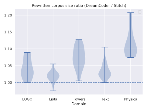
Figure 7. Compression rates obtained when running Stitch on the five domains considered in 6.1 relative to those of DreamCoder. Higher is better for Stitch: a ratio above 1.0 indicates that Stitch achieves greater compression than DreamCoder. The specific compression metric used in the ratio is given in Eq. 18.

Figure 8. Peak memory usage of Stitch and DreamCoder while running on the five domains considered in 6.1, averaged over all benchmarks. Lower is better; black lines indicate $\pm$ one standard deviation. Note the logarithmic y-axis.

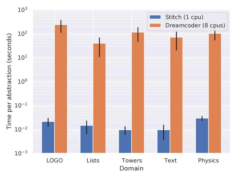
Figure 9. Wall-clock time required to find (and rewrite under) one abstraction in each of the five domains from 6.1, averaged over all benchmarks. Lower is better; black lines indicate $\pm$ one standard deviation. Note the logarithmic y-axis.

Results

We compare DreamCoder and Stitch for library quality and resource efficiency.

Library quality. We first examine the quality of the libraries learned by both Stitch and DreamCoder using the compression metric in Eq. 18: Fig. 7 shows the ratio between them across all of the benchmarks for each domain. A ratio of 1.0 indicates that programs are the exact same length under the libraries learned by DreamCoder and Stitch, a ratio greater than 1.0 indicates that Stitch learns more compressive libraries, and a ratio less than 1.0 indicates that Stitch learns libraries which are less compressive. For example, a ratio of 1.1 indicates that DreamCoder rewrote to produce a corpus 10% larger than that of Stitch, so it achieved less compression.

These results show that Stitch generally learns libraries of comparable and often greater quality than DreamCoder when matching the number of abstractions learned by the latter. In the logo, towers, text, and physics domains, Stitch always finds abstractions that are of equal—and often considerably greater—compressive quality than DreamCoder does; in the list domain, Stitch more often than not still obtains better compression, but sometimes loses out to DreamCoder. This is a result of the fact that Stitch cannot learn higher-order abstractions, which are useful in this domain; although we emphasize our focus is on scalability, we will later present an extension of Stitch capable of handling most higher-order functions in Section 6.5, based on the formalism developed in Section 5. Nonetheless, we conclude that Stitch learns libraries whose quality is comparable to and often better than those found by DreamCoder.

Resource efficiency. In addition to the quality of the libraries found, we are interested in how the two methods compare in terms of time and space requirements. Since we a priori believe Stitch to be significantly faster, for this evaluation we allow DreamCoder to use 8 CPUs but limit Stitch to single threading. The results are shown in Fig. 9 and Fig. 9; in summary, we find that Stitch takes tens of milliseconds to discover abstractions across all five domains—achieving a 3-4 order of magnitude speed-up over DreamCoder—while also requiring more than 2 orders of magnitude less memory. We thus conclude that Stitch is dramatically more efficient than the state-of-the-art deductive baseline when replicating the iterative library learning experiments of Ellis et al. 2021.

6.2. Large-Scale Corpus Library Learning

Experimental setup.

While the previous experiment allowed us to benchmark Stitch directly against a state-of-the-art deductive baseline, the iterated learning setting considered by Ellis et al. 2021 only evaluates library learning on relatively small corpora of short programs discovered by the synthesizer. Our second experiment is instead designed to evaluate Stitch in a more traditional learning setting, in which we aim to learn libraries of abstractions from a large corpus of existing programs all at once.

We source our larger-scale program datasets from Wong et al. 2022, which present a series of datasets designed as a benchmark for comparing human-level abstraction learning and graphics program writing against automated synthesis and library learning models. These datasets are divided into two distinct high-level domains (technical drawings and block-tower planning tasks), each consisting of four distinct subdomains containing 250 programs:

• Technical drawing domains: nuts and bolts; vehicles; gadgets; furniture: CAD-like graphics programs that render technical drawings of common objects, written in an initial DSL consisting of looped transformations (scaling, translation, rotation) over simple geometric curves (lines and arcs).

• Tower construction domains: bridges; cities; houses; castles: Planning programs that construct complex architectures by placing blocks, written in an initial DSL that moves a virtual hand over a canvas and places horizontal and vertical bricks.

We choose these datasets not only for their size and scale (full dataset statistics in Table 1), but also for the complexity of their potential abstractions: Wong et al. 2022 explicitly design their corpora to contain complex hierarchical structures throughout the programs, making them an interesting setting for library learning.

Domain	#Programs	Average program length	Average program depth
nuts & bolts	250	$76.03\pm 24.22$	$15.18\pm 2.13$
gadgets	250	$142.85\pm 87.32$	$20.88\pm 2.37$
furniture	250	$171.74\pm 48.41$	$31.83\pm 5.33$
vehicles	250	$141.70\pm 40.23$	$21.22\pm 1.35$
bridges	250	$137.03\pm 59.71$	$92.35\pm 39.80$
cities	250	$161.70\pm 55.56$	$109.80\pm 37.66$
castles	250	$189.09\pm 60.18$	$128.27\pm 40.77$
houses	250	$168.13\pm 55.75$	$114.85\pm 37.60$

Table 1. Summary statistics about the domains from Wong et al. 2022. Program length is the number of terminal symbols in the program; program depth is the length of the longest path from root to leaf in the program tree. Both are reported as the mean over the entire dataset $\pm$ one standard deviation.

When performing library learning in a synthesis setting by compressing a corpus of solutions, it’s desirable to find abstractions that would be useful for solving new tasks, as opposed to abstractions that overfit to the existing solutions. To evaluate how well the abstractions we learn apply to heldout programs in the domain, we split the corpora into train and test sets, running Stitch on the train set and evaluating its compression on the test set. Since Wong et al. 2022 do not present a train/test split of their datasets, we use stochastic cross validation to evaluate the generalization of the libraries found by Stitch. For each domain, we randomly sample 80% of the dataset to train on and reserve the last 20% as a held out test set; we repeat this procedure 50 times. We then ask Stitch to learn a library consisting of $\leq 10$ abstractions with a maximum arity of 3, and average the results across the different random seeds.

To obtain a baseline to compare its performance against, we once again turned to DreamCoder (Ellis et al., 2021). However, we found that DreamCoder was unable to discover even a single abstraction when run directly on any of the datasets from Wong et al. 2022, despite being given hours of runtime and 256GB of RAM. We also experimented with heavily sub-sampling the training dataset before passing it to DreamCoder, but failed to find a configuration under which DreamCoder finds any interesting abstractions at all due to the fact that it immediately blows up on programs as long as these. As a result, we resort to presenting Stitch’s performance metrics without any baseline to compare against; we stress that this is a direct result of the fact that Stitch is the first library learning tool that scales to such a challenging setting.

Results

Domain	Compression Ratio		Runtime (s)	Peak mem. usage (MB)
	Training set	Test set
nuts & bolts	$12.00\pm 0.25$	$11.57\pm 0.49$	$0.24\pm 0.04$	$11.10\pm 0.17$
gadgets	$4.03\pm 0.15$	$3.91\pm 0.31$	$1.83\pm 0.35$	$30.11\pm 0.85$
furniture	$4.95\pm 0.07$	$4.85\pm 0.26$	$2.83\pm 0.49$	$30.88\pm 0.62$
vehicles	$4.28\pm 0.14$	$4.14\pm 0.25$	$1.52\pm 0.29$	$26.98\pm 0.88$
bridges	$4.36\pm 0.06$	$3.78\pm 0.14$	$17.58\pm 1.26$	$189.08\pm 10.10$
cities	$3.15\pm 0.05$	$3.06\pm 0.14$	$50.74\pm 3.96$	$413.63\pm 9.51$
castles	$2.57\pm 0.07$	$2.55\pm 0.08$	$77.26\pm 6.98$	$683.89\pm 32.96$
houses	$8.92\pm 0.21$	$8.85\pm 0.57$	$15.54\pm 1.37$	$241.17\pm 2.86$

Table 2. Results for the large-scale library learning experiment in Sec. 6.2. The compression ratio refers to how many times smaller the corpus is after rewriting under the learned library compared to the original corpus; higher is thus better. All results are given as the mean $\pm$ one standard deviation over 50 runs with different random seeds for the dataset splitting.

The results are summarized in Table 2. We find that Stitch  scales up to even the most complex sub-domains, running in 77 seconds with a peak memory usage below 1GB on castles. On four out of eight of the domains, Stitch finishes in single-digit seconds and consumes only tens of megabytes. This stands in stark contrast to DreamCoder, which we were unable to run on the very simple nuts & bolts domain even with 256GB RAM and several hours worth of compute budget. These results thus support our claim that Stitch scales to corpora of programs that would be intractable with prior library learning approaches.

We hope that by providing our results on these datasets in full, future work in this field will benefit from having a directly comparable baseline.

6.3. Robustness to Early Search Termination

Experimental setup

This experiment is designed to evaluate how early into the search procedure Stitch finds what will eventually prove to be the optimal abstraction. This is highly relevant in settings where the set of training programs is too large to run the search to completion. The experiment showcases one of Stitch’s more subtle strengths: corpus-guided top-down abstraction search is an anytime algorithm, and thus does not need to be run to completion to give useful results.

We re-use the domains from Wong et al. 2022 and once again evaluate the quality of the library learned (measured in program compression), similarly to what was done in the previous experiment. However, since we are interested in how quickly Stitch finds what it perceives to be the optimal abstraction, we measure compressivity of the training dataset itself (rather than a held-out test set) and capture the compression ratio obtained by each candidate abstraction found during search (rather than just the compression ratio obtained when search has been run to completion). Thus, we are able to investigate how early on during the search procedure Stitch converges on a chosen library. We restrict Stitch to learning a single abstraction with a maximum arity of 3.

Results

Figure 10. Reduction in size obtained on the training set when rewritten under the best abstraction found thus far vs. the number of nodes expanded during search. The y-axis is normalized with respect to the optimal abstraction; the x-axis is normalized with respect to the total number of nodes explored by Stitch. Lines thus end earlier the quicker Stitch finds the optimal abstraction; however in all runs Stitch continues to search until reaching 100% on the x-axis, exploring the rest of the abstraction space without finding a new best abstraction. Note the logarithmic x-axis.

The results are shown in Fig. 10. These results validate our hypothesis that Stitch is empirically robust to terminating the search procedure early: in every sub-domain except for nuts & bolts Stitch converges to the optimal abstraction very early on, having only completed a tiny fraction of the total search. We believe that this has great importance for Stitch’s applicability in data-rich settings since it suggests that a nearly-optimal abstraction can be found even if the search must be terminated early (e.g. after a fixed amount of time has passed), making early stopping an empirically useful way of speeding up the library learning process.

6.4. Ablation Study

Experimental setup

Stitch implements several different optimizations, which we have argued hasten the search for abstractions. To verify that this claim holds in practice, we now carry out a brief ablation study.

Since the space of every possible combination of optimizations is too large to present succinctly, we focus our attention on four ablations:

• no-arg-capture (from Section 4.3), which disables the pruning of abstractions which are only ever used with the exact same set of arguments (and these arguments could therefore just be in-lined for greater compression).

• no-upper-bound, which disables the upper bound based pruning.

• no-redundant-args (from Section 4.3), which disables the pruning of multi-argument abstractions that have a redundant argument that could be removed because it is always the same as another argument.

• no-opts, which disables all of Stitch’s optimizations.

To isolate the impact of disabling optimizations, we run a single iteration of abstraction learning on each of the 8 domains from 6.2 and collect the number of nodes explored during the search. The first iteration is generally the most challenging as the corpus is large and has not yet been compressed at all. Focusing on the number of nodes explored (rather than for example runtime) allows for deterministic results. We also fix the maximum arity of abstractions to 3 in all runs, aiming to strike a good balance between compute requirements and how much the optimization will be exposed. We limit each run to 50GB of virtual address space, as well as 90 minutes of compute.

	bridges	castles	cities	gadgets	furniture	houses	nuts & bolts	vehicles
no-arg-capture				16714.28			30.21	26.67
no-upper-bound	12.15	23.71	27.90	207.76	119.00	36.18	179.12	179.99
no-redundant-args	1.95	1.42	1.37	1.01	1.00	1.01	1.09	1.00
no-opt

Table 3. Results from the ablation study. Each cell contains the ratio between the number of nodes explored during search by that particular system and the number of nodes explored by the baseline on the same domain. Lower is better; 1.00 means performance is identical to the baseline. Cells labeled  crashed due to reaching the 50GB virtual address space limit, while those labeled     reached the 90 minute time restriction.

Results

The results are shown in Table 3. We first note as a sanity check that each ablation does indeed lead to reduced performance in general (i.e. explores a search space larger than the baseline does). Furthermore, the results suggest that upper bound based pruning is the most important in the nuts & bolts and vehicles domains, while pruning out argument capture abstractions is the most important in the other six domains; it is noteworthy that this latter ablation by itself causes Stitch to reach the memory limit on more than half of the domains. On the other hand, disabling the pruning of redundant arguments has a relatively modest impact on the size of the search space, but still leads to an almost 2x improvement in the bridge domain.

Perhaps the most important takeaway from this ablation study is that when all optimizations are disabled, Stitch fails to find an abstraction within the resource budget on any of the domains. This verifies our hypothesis that corpus-guided pruning of the search space is the key factor involved in making top-down synthesis of abstractions tractable.

6.5. Learning Libraries of Higher-Order Functions

Experimental setup

Our experiments up till now have focused on performant and scalable library learning. This comes at the expense of some expressivity: deductive rewrite systems can, in principle, express broader spaces of refactorings. For example, a rewrite based on inverting $\beta$-reduction allows inventing auxiliary $\lambda$-abstractions, which helps with learning higher-order functions: in Ellis et al. 2021, DreamCoder is shown to recover higher-order functions such as map, fold, unfold, filter, and zip_with, starting from the Y-combinator. This works by constructing a version space which encodes every refactoring that is equivalent up to $\beta$-inversion rewrites. But DreamCoder’s coverage comes at a steep cost as inverting $\beta$-reduction is expensive.

In this experiment, we seek to give evidence that it is possible to make Stitch recover all of these higher-order functions by layering it on top of the version space obtained after a single step of DreamCoder’s $\beta$-inversion, following the formalism outlined in Section 5. We then compare this modified version of Stitch with DreamCoder on its ability to learn these higher-order functions from programs generated by intermediate DreamCoder iterations, and measure the runtime of each approach.

Probabilistic Re-ranking

While the approach outlined in Section 5 should suffice to layer Stitch on top of deductive rewrite systems based on version spaces, some extra care needs to be taken to combine it with DreamCoder. This is because DreamCoder implements a probabilistic Bayesian objective for judging candidate abstractions (exploiting the connection between compression and probability (Shannon, 1948)), seeking the library $L$ which maximizes $P(L)\prod_{p\in\mathcal{P}}P(p|L)$ for a given or learned prior $P(L)$ and program likelihood $P(p|L)$. Stitch, on the other hand, effectively judges compression quality via a cost function capturing the (weighted) size of the programs as detailed in Section 4.

To implement this probabilistic heuristic in Stitch, we simply run Stitch on the version spaces as-is but then re-score each complete abstraction popped off of the priority queue under the Bayesian objective, using DreamCoder’s models of the prior and likelihood. To make this integration easier, we re-implement Stitch in Python, giving a prototype version called pyStitch which is only used for this experiment. Our implementation employs strict dominance pruning, and prunes using the bound on the approximate utility given in Section 5.

System		Fold	Unfold	Map	Filter	ZipWith	Time (s)
	Base	✓	$\times$	✓	$\times$	✓	503
	+Bayes	✓	$\times$	✓	$\times$	✓	817
	+VS	✓	✓	✓	$\times$	✓	3231
pyStitch	+Bayes+VS	✓	✓	✓	✓	✓	3042
DreamCoder	Step 1	$\times$	$\times$	✓	$\times$	✓	67
	Step 2	$\times$	$\times$	✓	✓	$\times$	116
	Step 3	$\times$	$\times$	✓	✓	✓	2254
	Step 4	✓	✓	✓	✓	✓	228048

Table 4. Comparing library learners on functional programming exercises. DreamCoder, $n$-steps: deductive baseline rewriting $n$ steps of $\beta$-reduction. pyStitch: Python reimplementation of Stitch, which enables better interoperability with DreamCoder’s version space algebra (+VS) and probabilistic models (+Bayes). pyStitch+VS+Bayes learns all of the same higher-order functions, using $<2\%$ of the compute.

Results

The results are shown in Table 4. We note first the large discrepancy in runtimes; running DreamCoder with 4 steps of rewriting takes roughly 2.5 days of compute on this domain, while even the slowest version of pyStitch still finishes in less than an hour. In terms of the number of higher-order abstractions found, DreamCoder only finds all five when run in its most expensive configuration; reducing the computation cost quickly decreases its expressivity. For pyStitch, the Bayesian re-ranking alone (pyStitch+Bayes) does not yield any improvements, while running it on the version spaces (pyStitch+VS) yields 4 out of 5 functions. However, it is only when these two adaptations are used in conjunction (pyStitch+Bayes+VS) that the Stitch-based method is able to find all of the higher-order functions.

In summary, we find that running CTS after a single step of version space rewriting and then probabilistically re-ranking the results suffices to recover the core higher-order functions that DreamCoder learns, while using $<$2% of its compute. We thus conclude that running Stitch on top of a deductive rewrite system reduces the expressivity gap, while retaining superior performance.

7. Related Work

Stitch is related to two core ideas from prior work: deductive refactoring and library learning systems, which introduce the idea of learning abstractions that capture common structure across a set of programs, but have largely been driven by deductive algorithms; and guided top-down program synthesis systems, which use cost functions to guide top-down enumerative search over a space of programs, but have largely been used to synthesize whole programs for individual tasks in prior work.

7.1. Deductive Refactoring and Library Learning

Recent work shares Stitch’s goal of learning libraries of program abstractions which capture reusable structure across a corpus of programs (Ellis et al., 2018, 2021; Dechter et al., 2013; Cropper, 2019; Shin et al., 2019; Allamanis and Sutton, 2014; Iyer et al., 2019; Wong et al., 2021; Jones et al., 2021). Several of these prior approaches also introduce a utility metric based on program compression in order to determine the most useful candidate abstractions to retain (Dechter et al., 2013; Ellis et al., 2021; Wong et al., 2021; Lázaro-Gredilla et al., 2019; Iyer et al., 2019).

Much of this this prior work follows a bottom-up approach to abstraction learning, combining a bottom-up traversal across individual training programs with a second stage to extract shared abstractions from across the training corpus. This approach includes systems that work through direct memoization of subtrees across a corpus of programs (Dechter et al., 2013; Lin et al., 2014; Lázaro-Gredilla et al., 2019); antiunification (caching tree templates that can be unified with training program syntax trees) (Ellis et al., 2018; Henderson, 2013; Hwang et al., 2011; Iyer et al., 2019); or by more sophisticated refactoring using one or more rewrite rules to expose additional shared structure across training programs (Ellis et al., 2018, 2021; Chlipala et al., 2017; Liang et al., 2010).

Many of the bottom up algorithms draw more generally on deductive synthesis approaches that apply local rewrite rules in a bottom-up fashion to program trees in order to refactor them — historically, to synthesize programs from a declarative specification of desired function (Burstall and Darlington, 1977; Manna and Waldinger, 1980). Deductive approaches to library learning, however, confront fundamental memory and search-time scaling challenges as the corpus size and depth of the training programs increases; prior deductive approaches such as (Ellis et al., 2018, 2021) use version spaces (Lau et al., 2003; Mitchell, 1977) to mitigate the memory usage during bottom-up abstraction proposal. Still, deductive approaches are challenging to bound and prune (unlike the top-down approach we take in Stitch), as they generally traverse individual program trees locally and must store possible abstraction candidates in memory before the extraction step.

Some prior work (Shin et al., 2019; Allamanis and Sutton, 2014) takes an MCMC-based approach with better scaling behavior than deductive rewrites, but differs from the goals of Stitch as they don’t address binders and focus on common syntactic fragments instead of well-formed functions.

7.2. Guided Top-Down Program Synthesis

Stitch uses a corpus-guided top-down approach to learning library abstractions that is closely related to recent guided enumerative synthesis techniques. This includes methods that leverage type-based constraints on holes (Feser et al., 2015; Polikarpova et al., 2016), over- and under-approximations of the behaviors of holes (Lee et al., 2016; Chen et al., 2020), and probabilistic techniques to heuristically guide the search (Balog et al., 2016; Ellis et al., 2020, 2021; Nye et al., 2021; Shah et al., 2020). These approaches have largely been applied in to synthesize entire programs based on input/output examples or another form of specification, in contrast to the abstraction-learning goal in our work (Allamanis et al., 2018; Balog et al., 2016; Chen et al., 2018; Ellis et al., 2018; Ganin et al., 2018; Koukoutos et al., 2017). Like Stitch  however, these approaches sometimes use cost functions (such as the likelihood of a partially enumerated program under a hand-crafted or learned probabilistic generative model over programs) in order to direct search towards more desirable program trees. However, Stitch’s cost function leverages a more direct relationship between partially-enumerated candidate functions and the existing training corpus, unlike the cost functions typically applied in inductive synthesis, which must be estimated from input/output examples.

7.3. Lambda-Aware Unification

The LambdaUnify procedure presented in Section 3 relates to prior work on unification modulo binders (Huet, 1975; Miller, 1991, 1992; Dowek et al., 1995, 1996).

Notion of beta-equivalence. This prior work is concerned with more general notions of equivalence modulo beta-reduction, while LambdaUnify is based on a restricted but fast syntax-driven equivalence. For example, in Dowek et al. 1996 one might try to unify $(\alpha\ \texttt{foo})$ with $(\texttt{foo})$ and get the two solutions: $[\alpha\to(\lambda.\ \$0)]$ and $[\alpha\to(\lambda.\ \texttt{foo})]$. In contrast, LambdaUnify will never introduce a $\lambda-$abstraction to create a higher order argument and thus $(\alpha\ \texttt{foo})$ and $(\texttt{foo})$ would not unify at all, since one is an application while the other is a primitive. Instead, higher order abstraction arguments are handled by combining the algorithm with a deductive approach when desirable as in Section 5. We also note that in $\textsc{LambdaUnify}(A,e)$ it is assumed that $e$ is an expression and thus does not contain abstraction variables, which further simplifies the approach compared to this prior work.

Handling of binders. Dowek et al. 1995 and Dowek et al. 1996 both employ de Bruijn indexed variables and therefore must similarly account for the shifting of variables in arguments when inverting beta reduction. While LambdaUnify handles this through DownshiftAll, Dowek et al. 1995 and Dowek et al. 1996 both converting their terms to the $\lambda\sigma-$calculus of explicit substitutions (Abadi et al., 1989) which allows them to insert upshifting operators at each abstraction variable location. This alternate handling of shifting is useful given the more general notion of equivalence they are considering, but is excessive for our simpler syntax-guided task.

Handling of holes. In $\textsc{LambdaUnify}(A,e)$ we allow $A$ to contain holes ?? which are allowed to violate index shifting rules during unification as they are considered unfinished subtrees of the abstraction. This is handled through the use of $\&i$ indices. While the special-case handling of holes in expressions is not directly part of this prior work, there are similarities between it and the Skolemization (Skolem, 1920) done in Miller 1992. Skolemization allows for lifting an existential quantifier (i.e. an abstraction variable or hole) above a universal quantifier (i.e. a lambda) by turning the abstraction variable or hole into a function of its local context — in essence piping the local context into the hole. In the context of the lambda calculus this is essentially a form of lambda lifting (Johnsson, 1985), which is the process of lifting a local function that contains free variables by binding the free variables as additional arguments to the function and passing them in at each call site. In Miller 1992 this is used for abstraction variables (as there are no holes) and aids in the more general notion of beta-equivalence they are dealing with, while for our purposes the $\&i$ variables suffice and don’t require extra manipulations of lambdas to thread in the local context.

7.4. Upper Bounds in Network Motifs

There is also an interesting connection between this work and prior work on finding network motifs (Milo et al., 2002), which are frequently-occurring subgraphs within a corpus of graphs. One approach to mining high-frequency motifs is based on growing a motif one edge at a time, much like we grow abstractions one node at a time during our search (Schreiber and Schwöbbermeyer, 2005; Kuramochi and Karypis, 2004, 2001). This approach makes use of the insight that the frequency of a motif will only decrease as it is grown, giving an upper bound on the frequency of any motif derived from it. While we employ a more complex compressive utility function than their frequency-based utility, our upper bound is based on a similar insight that larger abstractions will match at a subset of the locations.

7.5. Comparison to babble

babble (Cao et al., 2023) is concurrent work in library learning that likewise adopts the compression objective from DreamCoder. While babble focuses primarily on expressive library learning through an algorithm that can reason over semantic equivalences represented through e-graphs, Stitch focuses primarily on efficient library learning through a parallel anytime branch-and-bound algorithm.

Stitch synthesizes the maximally-compressive abstraction for a corpus of programs through a branch-and-bound top-down search, computing an upper bound on the compression of any partially-constructed abstraction to guide and prune the search. In contrast, babble operates on an e-graph representing many equivalent corpora and uses anti-unification to propose candidate abstractions and a custom e-graph beam-search extraction algorithm to select a maximally-compressive set of abstractions from the proposal.

At a high level, Stitch aims to be efficient while babble aims to be expressive. The key differences between the algorithms are:

• Efficiency: On DreamCoder’s benchmarks, babble is 10-100x faster than DreamCoder while Stitch  is 1,000-10,000x faster than DreamCoder. Unlike babble, Stitch is an anytime algorithm that can be stopped early for a best-so-far result.

• Expressivity: babble can learn libraries modulo equational theories, allowing it to find common semantic abstractions despite syntactic differences in the programs. Stitch only explores non-syntactic equivalences preliminarily in the PyStitch prototype with the DreamCoder beta-inversion rewrite rule (Section 5 and Section 6.5).

• Jointly learning a library: babble can learn multiple abstractions at once that jointly provide compression, while DreamCoder and Stitch  repeatedly learn a single abstraction at a time. Stitch  provides an optimality guarantee on each abstraction learned while babble approximates the joint objective through a beam search.

These two approaches has advantages and disadvantages, and we believe that there is strong potential in combining the two.

8. Conclusion and Future Work

We have presented corpus-guided top-down synthesis (CTS)—an efficient new algorithm for synthesizing libraries of functional abstractions capturing common functionality within a corpus of programs. CTS directly synthesizes the abstractions, rather than exposing them through a series of rewrites as is done by deductive systems. Key to its performance is the usage of a guiding utility function, which allows CTS to effectively search (and prune out large portions of) the space of possible abstractions.

We implement this algorithm in Stitch, an open-source library learning tool with an associated Python library and Rust crate. We evaluate Stitch across five experimental settings, demonstrating that it learns comparably compressive libraries with 2 orders of magnitude less memory and 3-4 orders of magnitude less time compared to the state-of-the-art deductive algorithm of Ellis et al. 2021. We also find that Stitch scales to learning libraries of abstractions from much larger datasets of deeper program trees than is possible with prior work, and that the anytime property of corpus-guided top-down search — abstractions discovered via top-down search are already compressive early in search and improve as it continues — offers the opportunity for high-quality library learning even in complex domains through early search termination.

There remain many open problems and exciting directions in abstraction learning. One major direction is extending the CTS approach to handle reasoning over more general deductive rewrite systems, like those encoded in egg (Willsey et al., 2021) as babble does (Cao et al., 2023) (also see Section 7.5). The PyStitch prototype presented in Section 5 only works with a single rewrite rule (beta-inversion) and uses an approximate utility without an optimality guarantee. This is because it is challenging to adapt the upper bound used by Stitch to version spaces or e-graphs due to the trade-off between the compression gained from equational rewrites and compression gained from abstraction learning.

The speedup afforded by Stitch may allow for new applications of abstraction learning as well, as it can now be used as an inexpensive subroutine that can be called much more frequently than prior algorithms. To further extend its range of applications, CTS could also be adapted to finding abstractions in data structures beyond program trees, such as dataflow DAGs and more general graph structures like molecules, if the bounds and matching can be adapted. Finally, while we work with fairly large lambda calculus programs in this work, there is a clear gap in scale between these programs and those in an actual codebase, so exploring applications of CTS to real-world code is an exciting direction.

Data Availability Statement

All source code can be found at https://github.com/mlb2251/stitch. An artifact for reproducing results in this work is available at https://github.com/mlb2251/stitch-artifact or alternatively a static version is available at https://zenodo.org/record/7151663 (Bowers et al., 2022).

Appendix A Corpus-guided top-down search: full algorithm

In this appendix, we give an expansive description of the full corpus-guided top-down search (CTS) algorithm to ease re-implementation.

The full algorithm is given in Algorithm 1. It takes as input a corpus of programs $\mathcal{P}$, a utility function $U_{\mathcal{P},\mathcal{R}}(A)$, and utility upper bound function $\bar{U}_{\mathcal{P},\mathcal{R}}(A_{\texttt{??}})$. The algorithm searches for and returns the complete abstraction $A_{best}$ that maximizes the utility function. The algorithm maintains a priority queue $Q$ of partial abstractions ordered by their utility upper bound (or alternatively a custom priority function), a best complete abstraction so-far $A_{best}$, and a corresponding best utility so far $U_{best}$ for that abstraction. The priority queue is initialized to hold the single-hole partial abstraction ??, from which any abstraction can be derived. $A_{best}$ and $U_{best}$ are initialized as the best arity-zero abstraction and corresponding utility (line 4), since arity-zero abstractions can be quickly and completely enumerated (each unique, closed subexpression in the corpus is an arity-zero abstraction).

We then proceed to the core loop of the algorithm from lines 6-31. At each step of this loop we pop the highest-priority partial abstraction $A_{\texttt{??}}$ off of the priority queue and process it. We discard $A_{\texttt{??}}$ if its utility upper bound doesn’t exceed our best utility found so far (lines 8-10). We then choose a hole $h$ in $A_{\texttt{??}}$ to expand with the procedure Choose-Hole. Choose-Hole can be a custom function; we find from preliminary experiments on a subset of the datasets that choosing the most recently introduced hole is effective in practice.

The algorithm then uses the procedure Expansions to iterate over all possible single step expansions of the hole $h$ in $A_{\texttt{??}}$, such as replacing the hole with + or with (app ?? ??). For each expanded abstraction $A_{\texttt{??}}^{\prime}$, it is easy to compute its set of match locations $\textsc{Matches}(\mathcal{P},A_{\texttt{??}}^{\prime})$ since we know this will be a subset of the match locations of $A_{\texttt{??}}$ (and these will be disjoint subsets, except when expanding into an abstraction variable $\alpha$). We can easily inspect the relevant subtree at each match location of the original abstraction to see which expansions are valid and which match locations will be preserved by a given expansion. Note that an expansion to a free variable can be pruned immediately, as any resulting abstraction will not be well-formed.

When expanding to an abstraction variable $\alpha$, if $\alpha$ is a new variable not already present in the partial abstraction, the set of match locations is unchanged. If $\alpha$ is an existing abstraction variable then this is a situation where the same variable is being used in more than one place, as in the square abstraction $(\lambda\alpha.\ \texttt{*}\ \alpha\ \alpha)$. In this case we restrict the match locations to the subset of locations where within a location all instances of $\alpha$ match against the same subtree. Additionally, if a maximum arity is provided then an expansion that causes the abstraction to exceed this limit is not considered.

When considering each possible expanded abstraction $A_{\texttt{??}}^{\prime}$, there is room for strong corpus-guidance. First, we don’t need to consider any expansions that would result in zero match locations since all abstractions in this branch of search will have zero rewrite locations per Lemma 2 (lines 13-15). Furthermore, we use $\bar{U}_{\mathcal{P},\mathcal{R}}(A_{\texttt{??}}^{\prime})$ to upper bound the utility achievable in this branch of search and discard it if it is less than our best utility so far (lines 16-18). Since each $A_{\texttt{??}}^{\prime}$ covers a disjoint set of match locations (except in the case of expanding into an abstraction variable), the set of match locations often drops rapidly and can allow for the calculation of a tight upper bound depending on the utility function. As a final step of pruning, if we can identify that $A_{\texttt{??}}^{\prime}$ is strictly dominated by some other abstraction $A_{\texttt{??}}^{\prime\prime}$, we may discard $A_{\texttt{??}}^{\prime}$ (lines 19-21). Note additionally that arity-zero abstractions were precomputed, then abstractions that match at a single location are safe to prune as well (as long as they don’t have free variables) as arity-zero abstractions are always superior for single match locations.

For any partial abstraction $A_{\texttt{??}}^{\prime}$ that has not been pruned, we then check whether it is a complete abstraction (there are no remaining holes) or whether it is still a partial abstraction. Partial abstractions get pushed to the priority queue ranked by their utility upper bound, and complete abstractions are used to update $A_{best}$ and $U_{best}$ if they have a higher utility than any prior complete abstractions.

Once there are no more partial abstractions remaining in the priority queue, the algorithm terminates. Note that since the algorithm maintains a best abstraction so-far, it can also be terminated early, making it an any-time algorithm. We also note that this algorithm is amenable to parallelization as it can be easily parallelized over the while loop on lines 6-31, especially since the algorithm remains sound even when the upper bound $U_{best}$ used pruning is not always up to date.

This algorithm can be iterated to build up a library of abstractions.

Finally note that in our implementation, we employ structural hashing to simplify equality checks between subtrees and avoid re-doing work on multiple identical copies of a subtree. Our complete implementation of CTS for compression is provided at https://github.com/mlb2251/stitch.

Algorithm 1 Corpus-guided top-down abstraction synthesis. Color-coded: Upper bound pruning, Zero-usage pruning, Strict dominance pruning

1:Corpus of input programs $\mathcal{P}$, utility function $U_{\mathcal{P},\mathcal{R}}(A)$, and utility upper bound function $\bar{U}_{\mathcal{P},\mathcal{R}}(A_{\texttt{??}})$

2:The maximally compressive abstraction $A_{best}$

3:$Q\leftarrow$ Priority-Queue { ?? } $\triangleright$ New priority queue with the single partial abstraction ??

4:$A_{best}\leftarrow\textsc{Best-Arity-Zero-Abstraction}(\mathcal{P})$ $\triangleright$ Initialize best abstraction so far

5:$U_{best}\leftarrow U_{\mathcal{P},\mathcal{R}}(A_{best})$

6:while $\text{non-empty}(Q)$ do

7:     $A_{\texttt{??}}\leftarrow\text{pop-max}(Q)$ $\triangleright$ Next partial abstraction to expand

8:     if  $\bar{U}_{\mathcal{P},\mathcal{R}}(A_{\texttt{??}})\leq U_{best}$ then

9:         continue $\triangleright$ Upper bound pruning

10:     end if

11:     $h\leftarrow\textsc{Choose-Hole}(A_{\texttt{??}})$ $\triangleright$ Choose a hole to expand

12:     for $(A_{\texttt{??}}^{\prime},M^{\prime})\in\textsc{Expansions}(A_{\texttt{??}},h,\mathcal{P})$ do $\triangleright$ abstraction $A_{\texttt{??}}^{\prime}$ and match locations $M^{\prime}$

13:         if  $\text{length}(M^{\prime})==0$ then

14:              continue $\triangleright$ No match locations in corpus

15:         end if

16:         if  $\bar{U}_{\mathcal{P},\mathcal{R}}(A_{\texttt{??}}^{\prime})\leq U_{best}$ then

17:              continue $\triangleright$ Upper bound pruning

18:         end if

19:         if  $\text{strictly-dominated}(A_{\texttt{??}}^{\prime},\mathcal{P})$ then

20:              continue $\triangleright$ Strict dominance pruning

21:         end if

22:         if  $\text{has-holes}(A_{e})$ then

23:              $Q\leftarrow Q\cup A_{\texttt{??}}^{\prime}$ $\triangleright$ add partial abstraction to heap

24:         else

25:              if  $U_{\mathcal{P},\mathcal{R}}(A_{\texttt{??}}^{\prime})>U_{best}$ then

26:                  $U_{best}\leftarrow U_{\mathcal{P},\mathcal{R}}(A_{\texttt{??}}^{\prime})$ $\triangleright$ new best complete abstraction

27:                  $A_{best}\leftarrow A_{\texttt{??}}^{\prime}$

28:              end if

29:         end if

30:     end for

31:end while

Appendix B proof of Correctness of LambdaUnify

As introduced in Section 3, $\textsc{LambdaUnify}(A,e)$ returns a mapping from abstraction variables and holes to expressions $[\alpha_{i}\to e_{i}^{\prime},\ \ldots,\ \texttt{??}_{j}\to u_{j}^{\prime},\ \ldots]$ such that

(19) $$(\lambda\alpha_{i}.\ \ldots\ \lambda\texttt{??}_{j}.\ \ldots A)\ e_{i}^{\prime}\ \ldots\ u_{j}^{\prime}\ \ldots=e$$

through beta reduction. The LambdaUnify procedure is given in Fig. 4 and the definition of beta reduction with a modified upshifting operator is given in Fig. 5.

We can write Eq. 19 in terms of substitution as

(20) $$[\alpha_{i}\to e_{i}^{\prime},\ \ldots,\ \texttt{??}_{j}\to u_{j}^{\prime},\ \ldots]\ \circ A=e$$

Which can in turn be written in terms of LambdaUnify as

(21) $$\textsc{LambdaUnify}(A,e)\circ A=e$$

To prove the correctness of LambdaUnify, we must show that Eq. 21 holds for all $A$ and $e$. We do this in two ways: a written proof (below) of our correctness theorem (Theorem B.1), and a machine-verifiable proof in Coq. The Coq proof is given in stitch.v in the supplementary material and was proven with CoqIDE 8.15.2. The meanings of the definitions and lemmas in the Coq proof are commented. The Coq proof differs from the written proof in places because encoding the proof in Coq required coming up with some representations that worked well for Coq, though these differences are limited. For example, the Coq proof requires fully formalizing the behavior of Merge and proofs related to it which is more simply explained in the written proof. When lemmas in the written proof below correspond directly to lemmas in the Coq proof, the corresponding Coq lemma is indicated in the written proof below.

B.1. Well-formedness

We formalize a notion of well-formedness to capture the set of expressions that are accessible starting from an expression with no $\&i$ variables then applying any series of upshifts and downshifts. We define $\text{WF}_{d}(e)$, the well-formedness of an expression $e$ at a depth $d$, as follows:

$$\text{WF}_{d}\ \lambda.b=\text{WF}_{d+1}\ b$$

$$\text{WF}_{d}\ (fx)=\text{WF}_{d}\ f\land\text{WF}_{d}\ x$$

$$\text{WF}_{d}\ \$i=\top$$

$$\text{WF}_{d}\ \&i=\begin{cases}\top,&\text{if }i<d\\ \bot,&\text{if }i\geq d\\ \end{cases}$$

$$\text{WF}_{d}\ t=\top,\ \text{for $t\in\mathcal{G}_{\texttt{sym}}$}$$

Note that trivially any expression $e$ without any $\&i$ variables is well formed, as $\&i$ variables are the only source of $\bot$ in this definition.

If every expression in a mapping $l$ is well-formed, we say that the mapping itself is well-formed, written $(\text{WFMap}\ l)$.

B.2. Relevant Lemmas

The following two lemmas show that upshifting and downshifting preserve well-formedness. In Coq these lemmas are upshift_wf and downshift_wf.

Lemma 3.

$\forall e.\ \forall d.\ \text{WF}_{d}\ e\implies\text{WF}_{d}\ \uparrow_{d}e$

Proof.

We proceed by induction on e.

Case $e=\lambda.\ b$. Our goal is

$$\text{WF}_{d}\ \uparrow_{d}\lambda.b$$

We can move $\uparrow_{d}$ and $\text{WF}_{d}$ into the lambda by unfolding their definitions to get

$$\text{WF}_{d+1}\ \uparrow_{d+1}b$$

We also have the premise $\text{WF}_{d}\ \lambda.b$, where we can likewise move the $\text{WF}_{d}$ into the lambda to get $\text{WF}_{d+1}\ b$. The inductive hypothesis $\forall d.\ \text{WF}_{d}\ b\implies\text{WF}_{d}\ \uparrow_{d}b$ can be instantiated with $d$ as $d+1$ to get $\text{WF}_{d+1}\ b\implies\text{WF}_{d+1}\ \uparrow_{d+1}b$, the conclusion of which is precisely our goal and the premise of which is precisely our other premise.

Case $e=f\ x$. Our goal is

$$\text{WF}_{d}\ \uparrow_{d}(f\ x)$$

We can move $\uparrow_{d}$ and $\text{WF}_{d}$ into the application by unfolding their definitions to get

$$(\text{WF}_{d}\ \uparrow_{d}f)\ \land(\text{WF}_{d}\ \uparrow_{d}x)$$

We can use our inductive hypotheses $\text{WF}_{d}\ f\implies\text{WF}_{d}\ \uparrow_{d}f$ to prove the left side of this conjunction if we can prove $\text{WF}_{d}\ f$. We have the premise that $\text{WF}_{d}\ (f\ x)$ from this overall induction case, which by definition of $\text{WF}_{d}$ can only be true if $\text{WF}_{d}\ f\land\text{WF}_{d}\ d$. Thus we can prove the left side of the conjunction, and the proof of the right side is identical with $f$ replaced by $x$ using the other inductive hypothesis.

Case $e=\$i$. Our goal is

$$\text{WF}_{d}\ \uparrow_{d}\$i$$

We will handle this in 2 cases:

• Case $i<d$.

  $$\text{WF}_{d}\ \uparrow_{d}\$i$$

  $$=\text{WF}_{d}\ \$i$$

  This is true because $i indices are always well-formed.

• Case $i\geq d$.

  $$\text{WF}_{d}\ \uparrow_{d}\$i$$

  $$=\text{WF}_{d}\ \$(i+1)$$

  This is true because $i indices are always well-formed.

Case $e=\&i$. Our goal is

$$\text{WF}_{d}\ \uparrow_{d}\&i$$

We will handle our goal in 2 cases:

• Case $i+1\neq d$.

  $$\text{WF}_{d}\ \uparrow_{d}\$i$$

  $$=\text{WF}_{d}\ \&(i+1)$$

  We know from our premise that $\text{WF}_{d}\ \&i$ which means $i<d$, so $i+1\leq d$. Combining this with our knowledge from the case branch that $i+1\neq d$, we know that $i+1<d$ which means that $\&(i+1)$ is well formed.

• Case $i+1=d$.

  $$\text{WF}_{d}\ \uparrow_{d}\&i$$

  $$=\text{WF}_{d}\ \$(i+1)$$

  This is true because $i indices are always well-formed.

Case $e=t$. Our goal is $\text{WF}_{d}\ \uparrow_{d}t$ which simplifies by definition of $\uparrow_{d}$ to $\text{WF}_{d}\ t$ which is true by definition of $\text{WF}_{d}$.

∎

Lemma 4.

$\forall e.\ \forall d.\ \text{WF}_{d}\ e\implies\text{WF}_{d}\ \downarrow_{d}e$

Proof.

We proceed by induction on e. The cases $e=t$, $e=(f\ x)$ and $e=\lambda.b$ are identical to those in Lemma 3 but with $\uparrow$ replaced with $\downarrow$ so they will be omitted.

Case $e=\$i$. Our goal is

$$\text{WF}_{d}\ \downarrow_{d}\$i$$

We will handle this in 3 cases:

• Case $i<d$.

  $$\text{WF}_{d}\ \downarrow_{d}\$i$$

  $$=\text{WF}_{d}\ \$i$$

  This is true because $i indices are always well-formed.

• Case $i>d$.

  $$\text{WF}_{d}\ \downarrow_{d}\$i$$

  $$=\text{WF}_{d}\ \$(i-1)$$

  This is true because $i indices are always well-formed.

• Case $i=d$.

  $$\text{WF}_{d}\ \downarrow_{d}\$i$$

  $$=\text{WF}_{d}\ \&(i-1)$$

  Since $i=d$ we know that $i-1<d$ which means $\&(i-1)$ is well-formed.

Case $e=\&i$. Our goal is

$$\text{WF}_{d}\ \downarrow_{d}\&i$$

which simplifies to

$$\text{WF}_{d}\ \&(i-1)$$

We know from our premise that $\text{WF}_{d}\ \&i$ so $i<d$ which means $i-1<d$ so $\&(i-1)$ is well-formed.

∎

The following lemma shows that upshifting is an inverse of downshifting. In Coq this lemma is upshift_downshift.

Lemma 5.

$\forall e.\ \forall d.\ \text{WF}_{d}\ e\implies\uparrow_{d}\downarrow_{d}e=e$

Proof.

We proceed by induction on $e$.

Case $e=\lambda.\ b$. Our goal is

$$\uparrow_{d}\downarrow_{d}\lambda.\ b=\lambda.\ b$$

By the definitions of $\uparrow_{d}$ and $\downarrow_{d}$ we can propagate them into the body of a lambda while incrementing $d$:

$$\lambda.\ \uparrow_{d+1}\downarrow_{d+1}b=\lambda.\ b$$

We also have the additional premise $\text{WF}_{d}\ \lambda.b$ which simplifies to $\text{WF}_{d+1}\ b$.

Since our inductive hypothesis $\forall d.\ \text{WF}_{d}\ b\implies\uparrow_{d}\downarrow_{d}b=b$ is universally quantified over $d$ we can instantiate it with $d+1$ in place of $d$ and discharge its precondition with our other premise $\text{WF}_{d+1}\ b$ to get $\uparrow_{d+1}\downarrow_{d+1}b=b$ and apply this to our goal to get

$$\lambda.\ b=\lambda.\ b$$

which is trivially true.

Case $e=f\ x$. Our goal is

$$\uparrow_{d}\downarrow_{d}(f\ x)=f\ x$$

By the definitions of $\uparrow_{d}$ and $\downarrow_{d}$ we can propagate them into both sides of the application:

$$(\uparrow_{d}\downarrow_{d}f)(\uparrow_{d}\downarrow_{d}x)=f\ x$$

We also have the additional premise $\text{WF}_{d}\ (f\ x)$ can be broken into the two premises $\text{WF}_{d}\ f$ and $\text{WF}_{d}\ x$.

We can then apply our inductive hypotheses $\forall d.\ \text{WF}_{d}\ f\implies\uparrow_{d}\downarrow_{d}f=f$ and $\forall d.\ \text{WF}_{d}\ x\implies\uparrow_{d}\downarrow_{d}x=x$ with these premises to rewrite our goal to

$$f\ x=f\ x$$

which is trivially true.

Case $e=\$i$. Our goal is

$$\uparrow_{d}\downarrow_{d}\$i=\$i$$

We will handle this in 3 cases:

• Case $i<d$.

  $$\uparrow_{d}\downarrow_{d}\$i=\$i$$

  Unfold definition of $\downarrow_{d}$

  $$\uparrow_{d}\$i=\$i$$

  Unfold definition of $\uparrow_{d}$

  $$\$i=\$i$$

• Case $i>d$.

  $$\uparrow_{d}\downarrow_{d}\$i=\$i$$

  Unfold definition of $\downarrow_{d}$

  $$\uparrow_{d}\$(i-1)=\$i$$

  Unfold definition of $\uparrow_{d}$ noting that $(i-1)\geq d$

  $$\$((i-1)+1)=\$i$$

  Simplify

  $$\$i=\$i$$

• Case $i=d$.

  $$\uparrow_{d}\downarrow_{d}\$i=\$i$$

  Unfold definition of $\downarrow_{d}$

  $$\uparrow_{d}\&(i-1)=\$i$$

  Unfold definition of $\uparrow_{d}$ noting that $(i-1)+1=d$

  $$\$((i-1)+1)=\$i$$

  Simplify

  $$\$i=\$i$$

Case $e=\&i$. Our goal is

$$\uparrow_{d}\downarrow_{d}\&i=\&i$$

Unfolding the definition of $\downarrow_{d}$ yields

$$\uparrow_{d}\&(i-1)=\&i$$

Since we know that $\text{WF}_{d}\ \&i$ by our premise, we know that $i<d$ so $(i-1)+1<d$ so $(i-1)+1\neq d$ so $\uparrow_{d}$ unfolds to:

$$\&((i-1)+1)=\&i$$

which simplifies to

$$\&i=\&i$$

which is trivially true.

Case $e=t$. Our goal is

$$\uparrow_{d}\downarrow_{d}t=t$$

Neither $\uparrow_{d}$ nor $\downarrow_{d}$ have any effect on a grammar primitive $t$, so this is trivially true.

∎

The following lemma shows that any result of LambdaUnify is a well-formed mapping. In Coq this lemma is called lu_wf.

Lemma 6.

$\forall A.\ \forall e.\text{WFMap}\ \textsc{LambdaUnify}(A,e)$

Proof.

This is a straightforward proof by induction. In the $\alpha_{i}$ and and $\texttt{??}_{i}$ cases LambdaUnify adds expressions from the original expression to the mapping, which are well-formed as they can’t contain $\&i$ variables. In the lambda case DownshiftAll shifts variables using $\downarrow$ which is guaranteed to preserve well-formedness by Lemma 4. In the application case merge simply combines mappings from the function and argument calls to LambdaUnify which are well-formed by induction, resulting in an overall well-formed mapping. ∎

The following lemma follows from Lemma 5 and shows that UpshiftAll is an inverse of DownshiftAll. In Coq this lemma is upshift_all_downshift_all.

Lemma 7.

$\text{WFMap}\ l\implies\textsc{UpshiftAll}(\textsc{DownshiftAll}(l))=l$

Proof.

Writing $l$ as $[\alpha_{i}\to\ e_{i}^{\prime},\ \texttt{??}_{j}\to\ u_{j}^{\prime},\ ...]$ and unfolding the definitions of UpshiftAll DownshiftAll we get:

$$[\alpha_{i}\to\ \uparrow_{0}\downarrow_{0}e_{i}^{\prime},\ \texttt{??}_{j}\to\ \uparrow_{0}\downarrow_{0}u_{j}^{\prime},\ ...]=[\alpha_{i}\to\ e_{i}^{\prime},\ \texttt{??}_{j}\to\ u_{j}^{\prime},\ ...]$$

This equality will hold if $\uparrow_{0}\downarrow_{0}u_{j}^{\prime}=u_{j}^{\prime}$ and $\uparrow_{0}\downarrow_{0}e_{i}^{\prime}=e_{i}^{\prime}$ for all $u_{j}^{\prime}$ and $e_{i}^{\prime}$. $\text{WFMap}\ l$ tells us that all expressions $u_{j}^{\prime}$ and $e_{i}^{\prime}$ are well-formed and thus satisfy the precondition of Lemma 5, which proves these equalities true.

∎

The following two lemmas allow us to ”forget” one side of a merge when it won’t have any effect on the substitution. In Coq the first lemma is merge_forget3 and the second is captured by the definition Compatible.

Lemma 8.

If $l_{1}$ is a mapping that binds every abstraction variable and hole in $A$, then $\textsc{merge}(l_{1},l_{2})\circ A=l_{1}\circ A$.

Proof.

$l_{1}$ already assigns to every abstraction variable and hole, and merging in $l_{2}$ can’t overwrite these assignments since merge fails when the same variable or hole is assigned to two different expressions. Thus merging in $l_{2}$ has no effect on the resulting expression from substitution. ∎

Lemma 9.

If $l_{2}$ is a mapping that binds every abstraction variable and hole in $A$, then $\textsc{merge}(l_{1},l_{2})\circ A=l_{2}\circ A$.

Proof.

This proof is identical in structure to Lemma 8. $l_{2}$ already assigns to every abstraction variable and hole, and merging in $l_{1}$ can’t overwrite these assignments since merge fails when the same variable or hole is assigned to two different expressions. Thus merging in $l_{1}$ has no effect on the resulting expression from substitution. ∎

The following lemma shows that any result of LambdaUnify satisfies the precondition of Lemma 9 and Lemma 8.

Lemma 10.

$\textsc{LambdaUnify}(A,e)$ returns a mapping that binds all abstraction variables $\alpha_{i}$ and all holes $\texttt{??}_{i}$ in $A$.

Proof.

This is a straightforward proof by induction. In the $\alpha_{i}$ and and $\texttt{??}_{i}$ cases LambdaUnify binds the variable and hole respectively, in the lambda case DownshiftAll has no effect on which abstraction variables are bound (and it binds all the variables in the body by induction), and in the application case merge results in combining the function and argument mappings (which bind all variables by induction) to result in a mapping which binds all variables that appear in both the function and argument. ∎

B.3. Correctness Theorem

In Coq this theorem is called correctness.

Theorem B.1.

$\forall A.\ \forall e.\ \textsc{LambdaUnify}(A,e)\circ A=e$

Proof.

We proceed by induction over the proof tree of $\textsc{LambdaUnify}(A,e)$.

Case U-AbsVar. Our goal is $\textsc{LambdaUnify}(A,\alpha)\circ\alpha=e$ which simplifies by definition of LambdaUnify to $[\alpha\to e]\circ\alpha=e$ which is true by the definition of substitution.

Case U-Hole. Our goal is $\textsc{LambdaUnify}(A,\texttt{??})\circ\texttt{??}=e$ which simplifies by definition of LambdaUnify to $[\texttt{??}\to e]\circ\texttt{??}=e$ which is true by the definition of substitution.

Case U-App. Our goal is

$$\textsc{LambdaUnify}(A_{1}\ A_{2},\ e_{1}\ e_{2})\circ(A_{1}\ A_{2})=e_{1}\ e_{2}$$

This simplifies by definition of LambdaUnify to

$$\textsc{merge}(\textsc{LambdaUnify}(A_{1},e_{1}),\textsc{LambdaUnify}(A_{2},e_{2}))\circ(A_{1}\ A_{2})=e_{1}\ e_{2}$$

We can distribute the substitution over the application (by definition of substitution in Fig. 5 (Left)) to get

$$( (\textsc{merge}(\textsc{LambdaUnify}(A_{1},e_{1}),\textsc{LambdaUnify}(A_{2},e_{2}))\circ A_{1})$$

$$(\textsc{merge}(\textsc{LambdaUnify}(A_{1},e_{1}),\textsc{LambdaUnify}(A_{2},e_{2}))\circ A_{2}))$$

$$=e_{1}\ e_{2}$$

We can then forget the irrelevant part of each merge using Lemma 9 and Lemma 8 where the precondition (binding all abstraction variables and holes) is satisfied by Lemma 10:

$$( (\textsc{LambdaUnify}(A_{1},e_{1})\circ A_{1})$$

$$(\textsc{LambdaUnify}(A_{2},e_{2})\circ A_{2}))$$

$$=e_{1}\ e_{2}$$

We can then finish the proof by directly applying our inductive hypotheses $\textsc{LambdaUnify}(A_{1},e_{1})\circ A_{1}=e_{1}$ and $\textsc{LambdaUnify}(A_{2},e_{2})\circ A_{2}=e_{2}$.

Case U-Lam. Our goal is

$$\textsc{LambdaUnify}(\lambda.\ A,\lambda.\ e)\circ\lambda.\ A=\lambda.\ e$$

This simplifies by definition of LambdaUnify to

$$\textsc{DownshiftAll}(\textsc{LambdaUnify}(A,e))\circ\lambda.\ A=\lambda.\ e$$

We can move the substitution under the lambda while inserting UpshiftAll as per the definition of substitution

$$\lambda.\ \textsc{UpshiftAll}(\textsc{DownshiftAll}(\textsc{LambdaUnify}(A,e)))\circ A=\lambda.\ e$$

Since we know that any result of LambdaUnify is well-formed by Lemma 6 we can apply Lemma 7 to get

$$\lambda.\ \textsc{LambdaUnify}(A,e)\circ A=\lambda.\ e$$

We can then apply our inductive hypothesis $\textsc{LambdaUnify}(A,e)\circ A=e$ to get

$$\lambda.\ e=\lambda.\ e$$

and we are done.

Case U-Same. Our goal is $\textsc{LambdaUnify}(e,e)\circ e=e$ which simplifies by definition of LambdaUnify to $[]\circ e=e$ which is trivially true as the empty substitution has no effect.

∎