Sequence learning in a spiking neuronal network with memristive synapses
Abstract
Brain-inspired computing proposes a set of algorithmic principles that hold promise for advancing artificial intelligence. They endow systems with self learning capabilities, efficient energy usage, and high storage capacity. A core concept that lies at the heart of brain computation is sequence learning and prediction. This form of computation is essential for almost all our daily tasks such as movement generation, perception, and language. Understanding how the brain performs such a computation is not only important to advance neuroscience but also to pave the way to new technological brain-inspired applications. A previously developed spiking neural network implementation of sequence prediction and recall learns complex, high-order sequences in an unsupervised manner by local, biologically inspired plasticity rules. An emerging type of hardware that holds promise for efficiently running this type of algorithm is neuromorphic hardware. It emulates the way the brain processes information and maps neurons and synapses directly into a physical substrate. Memristive devices have been identified as potential synaptic elements in neuromorphic hardware. In particular, redox-induced resistive random access memories (ReRAM) devices stand out at many aspects. They permit scalability, are energy efficient and fast, and can implement biological plasticity rules. In this work, we study the feasibility of using ReRAM devices as a replacement of the biological synapses in the sequence learning model. We implement and simulate the model including the ReRAM plasticity using the neural simulator NEST. We investigate two types of ReRAM devices: (i) an analog switching memristive device, where the conductance gradually changes between a low conductance (LCS) and a high conductance state (HCS), and (ii) a binary switch memristive device, where the conductance abruptly changes between the LCS and the HCS. We study the effect of different device properties on the performance characteristics of the sequence learning model, and demonstrate resilience with respect to different on-off ratios, conductance resolutions, device variability, and synaptic failure.
1 Introduction
In everyday’s tasks such as learning, recognizing, or predicting objects in a noisy environment, the brain outperforms conventional computing systems and deep learning algorithms at many aspects: it has a higher capacity to generalize, can learn from small training examples, is robust with respect to perturbations and failure, and is highly resource and energy efficient. To achieve this performance, it uses intricate biological mechanisms and principles. Understanding these principles is essential for driving new advances in neuroscience and for developing new real-world applications. For instance, it is known that biological neural networks are highly sparse in activity and connectivity and they can self-organize in the face of the incoming sensory stimulus using unsupervised local learning rules. A number of biologically inspired algorithms relying on these principles have been developed for sequence prediction and replay (Lazar et al., 2009; Hawkins and Ahmad, 2016; Bouhadjar et al., 2022b), pattern recognition (Masquelier and Thorpe, 2007; Payeur et al., 2021), and decision making (Neftci and Averbeck, 2019). The spiking temporal memory (spiking TM) network proposed by Bouhadjar et al. (2022b) learns high-order sequences in an unsupervised, continuous manner using local learning rules. Owing to its highly sparse activity and connectivity, it provides an energy-efficient sequence learning and prediction mechanism.
The spiking TM algorithm was originally implemented using the neural simulator NEST (Gewaltig and Diesmann, 2007). While NEST provides a simulation platform optimized for running large-scale networks efficiently in a reproducible manner, it is executed on standard von-Neumann-type computers, i.e., on hardware that is not specifically optimized for neuromorphic computing. This results in performance limitations as the simulation time and the energy dissipation become substantially high for brain-scale neural networks (Kunkel et al., 2014; Jordan et al., 2018). For using spiking TM in edge-computing applications, more efficient hardware is therefore required. Neuromorphic hardware, with dedicated solutions to the high demands imposed by the natural-density connectivity of the brain and the resulting communication load, as well as, specific circuit blocks emulating neuron and synapse functionalities, present a potential solution for that (Burr et al., 2016; Xia and Yang, 2019; Marković et al., 2020; Zhu et al., 2020). The local learning rules and the sparse neuronal activation of the spiking TM model allow for efficient mapping of the algorithm on neuromorphic hardware.
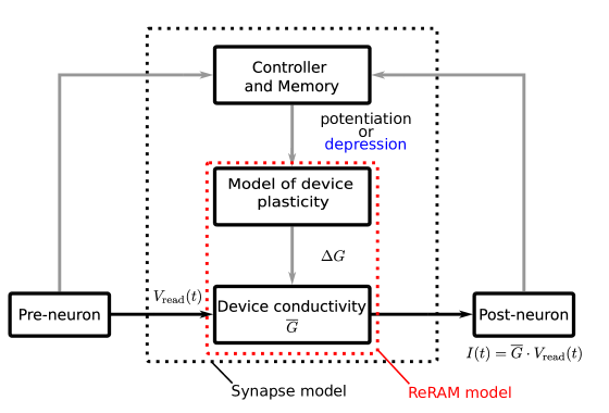
Memristive devices were suggested as components in such a hardware (Yang et al., 2013; Ielmini and Wong, 2018; Yu, 2018). They can be used to emulate certain synaptic functionalities using only a single device, by replacing more complex CMOS-based circuits (Waser et al., 2009; Dittmann and Strachan, 2019). Their intrinsic dynamics capture similar characteristics as the biological synapses such as variability, weight dependence of the update, and nonvolatility. However, while single memristive devices may readily emulate the inference function, they cannot emulate on their own plasticity rules such as spike-timing-dependent plasticity (STDP) or homeostatic control. The change of the memristive conductivity depends on the momentary voltage difference between its two terminals, and the device has no memory of past spike events at either of its terminals nor of their relative timing. Hebbian learning such as STDP therefore can only be emulated using a memristive device by “reshaping” of the pre- and post-synaptic spike events using complex voltage pulses, so that the spike-time dependency is translated into a desired instantaneous voltage difference over the device (Zamarreño-Ramos et al., 2011; Wang et al., 2015). As a result, the learning rule is controlled outside the actual device (see fig. 1). As for implementing the learning, instead of using complex voltage pulse shapes, it is more efficient to use a controller to generate simple rectangular voltage pulses that can effectuate the desired change of the device conductance in a better, more energy efficient, and also more reliable way. The change of the device conductivity as a function of the number of applied voltage pulses can hereby be seen as an intrinsic plasticity curve of the device, where the actual pulse shape can be optimized towards desired potentiation and depression characteristics.
In this work, we investigate how the intrinsic potentiation and depression characteristics of memristive devices influence the learning of the model in (Bouhadjar et al., 2022b). Thereto, we adapt the original neuroscientific synapse model to accommodate memristive-type potentiation/depression characteristics. The performance of the system is assessed by varying device characteristics such as conductance values and ranges, granularity of conductance change, and device variability. In this work, we study a particular type of memristive device known as the valence change memory (VCM) ReRAM device (Waser, 2012b). We investigate its two operation modes (Cüppers et al., 2019): either the continuous, analog mode, where the conductivity changes gradually between a Low conductance state (LCS) and a high conductance state (HCS), or the binary mode, where the conductivity changes abruptly between the LCS and the HCS. The binary switching is controlled by the value of an analog adaptable internal state variable (Doevenspeck et al., 2018; Zhao et al., 2019; Suri et al., 2013; Yu, 2018). It resembles the learning rule employed in (Bouhadjar et al., 2022b) and mimics a structural form of STDP known in the neuroscientific literature.
2 Results
2.1 A synapse model for ReRAM devices
In this section, we briefly review the ReRAM device dynamics, introduce our model of the ReRAM device and its control circuitry, and characterize the resulting model dynamics.
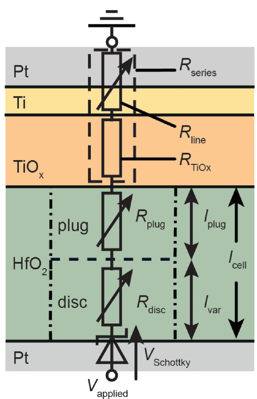
The VCM ReRAM device consists of a thin (–) insulating transition metal-oxide film sandwiched between a low work function (WF), ohmic electrode, and a high WF, blocking Schottky-interface electrode (see fig. 2). In a first step, a conductive filament is formed due to a high voltage applied across the device. This filament consists of oxygen vacancies that act as local dopant elements in the insulating metal-oxide matrix. During further operation, these oxygen vacancies can be moved by means of a high electric field and a local Joule heating (as a function of the polarity, either towards or away from the blocking electrode). The device conductance is controlled by the concentration of oxygen vacancies in a small region (gap) near the electrical blocking electrode: at low , the filament is “broken”, which gives rise to a high conduction barrier between the high WF electrode and the remaining filament (plug), i.e., the device is in the LCS. If is high, we have a “connecting” filament, where the high lowers the conduction potential barrier at the blocking electrode, i.e., the device is in the HCS. Hence, the concentration of the oxygen vacancies can be seen as an internal state variable of the device.
As mentioned above, depending on the initial resistance range and the voltage pulse amplitude and width, a VCM ReRAM device can operate in two different modes, i.e., binary or analog (Cüppers et al., 2019). In the analog mode, the applied pulses result in a gradual monotonous change of the device conductance, for both potentiation and depression. This operation mode is suitable for the implementation of STDP-type learning rules. It is, however, characterized by a limited conductivity range, and the device switching characteristics may slowly drift away from the analog behavior to a more abrupt conductivity change. In the binary mode, the conductivity can only be switched between two values, the LCS and the HCS. The switching between these two states occurs abruptly. In previous works, the abrupt, binary switching is achieved using single program pulses with a sufficiently large amplitude (Cüppers et al., 2019). In contrast, here, we study the switching behavior of the device as a response to a certain number of pulses of smaller amplitudes. As a response to these pulses, an internal state variable gradually increases (Fleck et al., 2016). Only when this exceeds a certain threshold value, a thermal runaway condition is reached resulting in an abrupt switching event. Due to intrinsic ReRAM device variabilities (Fantini et al., 2013), the number of pulses to reach this thermal runaway conditions shows a strong device-to-device and cycle-to-cycle variation. During the depression, the switching is intrinsically more gradual, due to the lack of an internal runaway mechanism as present for the potentiation operation. Adding a series resistance (in or outside the device) can provide such runaway mechanism due to a voltage divider effect also in the RESET case (Hardtdegen et al., 2018). Hence, in both cases, the switching behavior can be summarized as follow: at first only a gradual change of the internal state variable is observed, associated with only a minor change of the device conductivity, followed by a strong switching effect (large change of as well as of the associated conductivity) when the internal state variable reaches a certain threshold. This operation mode is of particular interest for this study, as it is similar to the structural STDP plasticity discussed and implemented in the original spiking TM model (Bouhadjar et al., 2022b).
Previous studies suggested both physics-based and phenomenological models for VCM type ReRAMs. Physics-based models such as the JART model (Bengel et al., 2020) capture detailed physical characteristics and predict their specific experimental behavior. They require however long simulation time and lead to convergence issues. On the other hand, the more phenomenological models give a high-level description of the operational characteristics, have good accuracy, are computationally less demanding, and can hence be combined with large-scale network models. In this study, we opt for a phenomenological model to implement both the analog and the binary ReRAM device.
The synapses are either potentiated or depressed by following learning rules similar to those outlined in the spiking TM model. The learning rules are implemented by the control circuit (fig. 1) as follows: the synapse is depressed slightly at every presynaptic spike and potentiated if a postsynaptic spike follows after a presynaptic spike. In contrast to the original spiking TM model, synapses are potentiated by a fixed amount irrespective of the relative timing between the pre- and postsynaptic spikes. The potentiation is however disabled if these spikes occur very close to each other within the interval [0, ]. This prohibits synchronously firing neurons from connecting to each other. The control circuit further implements a homeostatic control mechanism (see section 2.2).
In the analog mode, the increment
| (1) |
in the conductivity of the device (synapse) following a potentiation or a depression event is modeled as in (Fusi and Abbott, 2007), but with an additional additive noise . For each synapse and for each potentiation and depression step, the noise is randomly and independently drawn from a normal distribution with zero mean and standard deviation . The conductance evolves between a lower and an upper bound and , and it is clipped at these boundaries, with learning rates and and weight dependence exponents and . The conductance changes linearly with the internal state variable , thus no specification of the internal state variable is necessary. The initial conductance is drawn for every new device from a uniform distribution in the interval [].
For the binary switching behavior, we use a similar model as the structural STDP model proposed by Bouhadjar et al. (2022b). The switching of the conductance between the LCS and the HCS is controlled by a permanence . The permanence plays the role of the internal state variable . If it is above a certain threshold , the conductance is set to , otherwise it is set to :
| (2) |
Similar to the analog synapse, the initial conductance is drawn for every new device from a uniform distribution in the interval []. At each potentiation or depression step, the permanence of the synapse is incremented by an amount
| (3) |
similar to the conductance increment of the analog synapse. It has a lower and an upper bound and and it is clipped at these boundaries. While the maximum permanences are identical for synapses, the minimal permanences are uniformly distributed in the interval .
In addition to the write noise introduced by means of the variable , both the analog and the binary synapse models incorporate a read noise. At each presynaptic spike of neuron , a noisy component Z is added to the synaptic current
| (4) |
of neuron , where is randomly and independently drawn from a normal distribution with zero mean and standard deviation , and is the applied voltage. In the course of this article, we use to denote the conductance incorporating both the read and the write noise.
Figure 3 shows an exemplary switching behavior of the analog and binary synapse models for a specific set of parameters using consecutive potentiation (i.e., SET) and depression (i.e., RESET) updates. We choose different learning rates ( and ) for the two types of devices such that they switch from the LCS to the HCS (and back) at about the same number of updates. Under normal operation of the spiking TM model, a potentiation update is always followed by a small depression (fig. 4A). In the case of the analog synapse, the total synaptic growth in the absence of noise is therefore governed by
| (5) |
The stationary solution of the device conductance (fixed point) , obtained by setting , is always below the maximum conductance (fig. 4B). The permanence of the binary synapse is subject to this effect, too. After a number of potentiation steps, it reaches a value smaller than (see fig. 4C). According to eq. 2, the conductance can however still assume . Only if the depression is too strong, the device may not reach the maturity threshold , and thus not switch to the HCS.
In the next sections, we evaluate the effects of different characteristics of the analog and the binary switching dynamics such as the weight dependence of the device update (, ), the conductance range (, ), the learning rates (, ), as well as the write and the read variability (, ) on the learning process of the spiking TM model.


2.2 A spiking neural networks with ReRAM synapses successful at sequence prediction
Sequence learning and prediction are principal computations performed by the brain and have a number of potential technological applications. The study by Bouhadjar et al. (2022b) proposed a model of this type of computation known as the spiking temporal memory (spiking TM) model. It consists of a sparsely and recurrently connected network of spiking neurons and learns sequences continuously in an unsupervised manner by means of known biological plasticity mechanisms. After learning, the network successfully predicts and recalls complex sequences in a context-specific manner, and signals anomalies in the data.
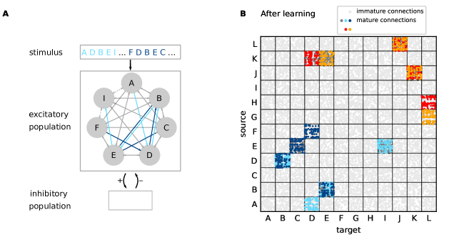
We briefly describe here the main mechanisms and principles of the spiking TM model. For an in-depth analysis, we refer readers to (Bouhadjar et al., 2022b). The model is composed of a excitatory (“E”) and inhibitory (“I”) neurons, which are randomly and sparsely connected. Excitatory neurons are subdivided into subpopulations of neurons, each representing a sequence element and sharing the same stimulus preference (fig. 5A). Excitatory neurons are recurrently connected to the inhibitory neurons implementing a winner-take-all (WTA) mechanism. We model neurons using leaky integrate-and-fire dynamics. Excitatory neurons are additionally equipped with nonlinear dendrites mimicking dendritic action potentials (dAPs). We model the dAPs as follows: if the dendritic current exceeds a threshold , it is instantly set and clamped to the dAP plateau current for a period of duration . The dAP threshold is chosen such that the co-activation of presynaptic neurons reliably triggers a dAP in the target neuron:
| (6) |
In the case of the analog synapse, is taken to be the steady-state conductance , and in the case of the binary synapse, it is taken to be . In a previous study, we show that it is also possible to model the dendrites using leaky integrate-and-fire dynamics (Bouhadjar et al., 2019). In addition to the dendritic input, the excitatory neurons are equipped with additional inputs from external and inhibitory sources. Inhibitory neurons have only a single excitatory input. The synapses between excitatory neurons are plastic evolving according to the analog or the binary ReRAM models described in section 2.1. A homeostatic component further controls the synaptic growth: if the dAP activity, i.e, the number of generated dAPs in a certain time window, is below a target , the synaptic weight is increased, otherwise, it is decreased (see section 5).
During the learning process, the network is repeatedly presented with a given ensemble of sequences. Before learning, presenting a sequence element causes all neurons in the respective subpopulation to fire, except the subpopulation representing the first sequence element, where only a random subset of neurons is activated. The repeated presentation of the sequences strengthens the connections between the subpopulations representing subsequently presented elements. After sufficient learning, the activation of a subpopulation by an external input causes a specific subset of neurons in the following subpopulation to generate dendritic action potentials (dAPs) resulting in a long-lasting depolarization of the somata. Neurons that generate dAPs signal the anticipated sequence element and are thus referred to as predictive neurons. When receiving an external input, predictive neurons fire earlier as compared to non-predictive neurons. If a certain subpopulation contains a sufficient number of predictive neurons, their advanced spike initiates a fast and strong inhibitory feedback to the entire subpopulation, ultimately suppressing the firing of the non-predictive neurons. The randomness in the connectivity supplemented by the homeostatic control enables the generation of sequence-specific sparse connectivity patterns between subsequently activated neuronal subpopulations (fig. 5A,B). For each pair of sequence elements in a given sequence ensemble, there is a unique set of postsynaptic neurons generating dAPs. Consequently, after learning in response to the presentation of a sequence element, the network predicts in a context-dependent manner the next element in the sequence by activating the dAPs of the corresponding subpopulation (fig. 5C,D).
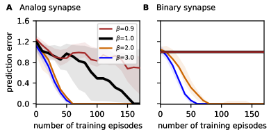
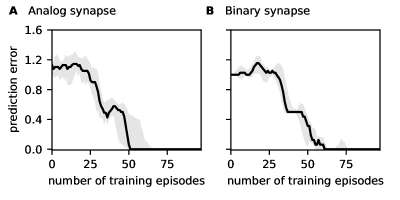
Here, we study the prediction performance for the network with either the binary or the analog ReRAM synapses (fig. 6). We use the synaptic parameters fitted from the exemplary data discussed in section 2.1. To quantify the sequence prediction performance, we repetitively stimulate the network using the same set of sequence , , , and assess the prediction error by comparing the the anticipated next sequence element with the correct one (Bouhadjar et al., 2022b). To ensure the performance results are not specific to a single network, the evaluation is repeated for a number of randomly instantiated network realizations with different initial connectivities. After each new network instantiation, the initial prediction error is at (fig. 6). With an increasing number of training episodes, the prediction error for both networks with either the binary or the analog synapses decreases to zero as both networks learn the sequences and develop context-dependent pathways between successive sequence elements.
2.3 Influence of device characteristics on prediction performance
ReRAM devices reported in the literature exhibit different nonidealities, including 1) limited precision or the number of synaptic levels; 2) limited dynamic range; 3) dependence of the synaptic updates on the weight, also known as synaptic nonlinearity; 4) device variability, including read and write variability (see Zhao et al., 2020, for an overview). In this section, we study how these nonidealities affect the prediction performance in the spiking TM model.
2.3.1 Optimal prediction performance obtained for a broad range of on-off ratios and learning rates
The dynamic range is defined as the on-off ratio between the minimum () and the maximum conductance (). Most ReRAM devices exhibit an on-off ratio in a range of x to x (Hong et al., 2018). Within the minimum and the maximum conductance, the synaptic precision or the number of synaptic steps is limited. In the synapse model proposed in section 2.1, we can influence the number of steps by changing parameters such as the learning rates (, ), weight dependence exponents (,), or the on-off ratio. Given the difficulty to derive an analytical solution of the number of steps as a function of these parameters, we restrict the scope of the study in this section to investigating the influence of different learning rates and on-off ratios on the prediction performance.
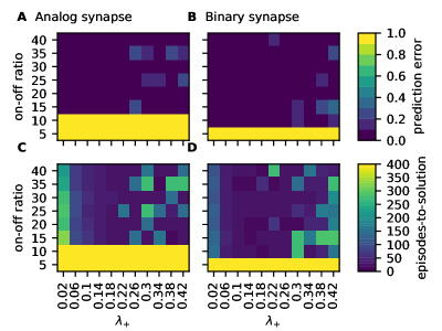
We vary the on-off ratio between and by keeping fixed and varying . As is drawn from a uniform distribution in the interval [, ], we compute the on-off ratio as , where . As we change , we modify the dAP threshold, see eq. 6. In addition, we vary the learning rate between and (fig. 7). Parameters such as the read and write variability and the weight dependence exponents are taken from the exemplary data presented in section 2.1. We study the influence of the variability and the dependence of the synaptic updates on the weight more systematically in the upcoming sections. For the analog synapse, the prediction error converges to zero for an on-off ratio between and and for a learning rate between and . For the binary synapse, successful learning is obtained for an on-off ratio between and and for a learning rate between and (fig. 7A,B). For learning rates above , the prediction performance becomes less stable with sudden failures for some network realizations. While decreasing the learning rate yields minimum prediction error, the number of episodes-to-solution tends to increase as either the conductances or permanences need more learning steps to reach their maximum value (fig. 7C,D). The learning in the network with binary synapses is faster due to the internal dynamics of binary synapses, which has faster switching dynamics compared to analog synapses: the permanence takes less number of update steps to reach the maturity threshold () compared to the number of update steps the conductance of the analog synapses require to go from the LCS to the HCS.
In general, the on-off ratio in the spiking TM network is limited due to the following: the transition of the network activity from being initially non-sparse to becoming sparse after learning requires initial small conductances to avoid spurious activation of the dAPs, but high conductances after learning to allow the sparse set of active neurons to generate the dAP reliably. If the on-off ratio is too small this distinction between high and small conductances cannot be realized. Moreover, for successful learning, the network with analog synapses requires a higher on-off ratio compared to the network with binary synapses. This is due to the effect described in section 2.1 below equation eq. 5, which prohibits the conductance from reaching . Therefore, the effective on-off ratio is reduced. The learning mechanisms of the spiking TM also limit the range of possible learning rates. Increasing the learning rate bears the risk that a large fraction of neurons reaches the dAP threshold at the same time. The WTA mechanism selects then all neurons that generate dAP to become active. This leads to a loss of sparseness, which results in impairing the prediction performance. Decreasing the learning rate considerably is also not ideal as the network would learn very slowly.
2.3.2 Resilience of the model against weight dependent updates
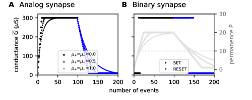
The evolution of the conductance of realistic analog synapses grows in a nonlinear manner as a function of the potentiation and depression updates. The synapse model in section 2.1 captures this effect via the weight dependence factor controlled by the exponents (, ). During the potentiation process, the conductance tends to change rapidly at the beginning but saturates at the end of the process (see fig. 8A). Similar behavior is also observed during the RESET. The potentiation and depression operations have, however, different dependencies on the device conductance. For high conductances, the potentiation increments are much smaller than the depression decrements. This asymmetry in the behavior can be further enhanced if the learning rates are different during the potentiation and depression operations. Similarly, it is reasonable to assume that for the binary synapses the evolution of the permanence may exhibit a nonlinear dependence on the synaptic updates and an asymmetric behavior between the potentiation and depression dynamics (fig. 8B).
Here, we first evaluate how the asymmetry in the learning rates between the potentiation and depression operations ( and ) affects the prediction performance. To study this effect, we fix and vary with the state dependence exponents and being set to zero. The prediction error remains high if (see fig. S1). This is due to the plasticity dynamics of the spiking TM model: the potentiation operation is applied only when the postsynaptic spike follows after the presynaptic spike, in contrast, the RESET operation is applied every time the presynaptic neuron generates a spike. Therefore, for effective synaptic growth, the potentiation needs to be stronger than depression.
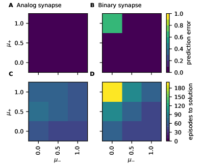
We assess, next, the prediction performance as a function of different weight dependence exponents for both potentiation and depression ( and , respectively, see fig. 9). The results show that this latter has mild effects on the prediction error (see fig. 9A,B). For larger values of , the learning speed slows down as it takes longer for either the conductance or the permanence to reach their maximum values (see fig. 9C,D). Decreasing makes learning faster again as the depression becomes weaker compared to the potentiation. In the binary case, the steady-state permanence may end up below the maturity threshold such that the synapses can mature only due to the noise. The learning is therefore slowed down for large values of or even unsuccessful if the devices do not switch to the HCS. In the model, could be adjusted to (similarly to adjusting to in the analog synapse; see above). In this case, the learning in the analog and the binary networks may be similarly fast. In the physical device, however, the maturity threshold can hardly be changed.
2.3.3 Resilience of the model against variability
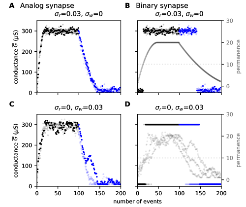
The resistive switching process of ReRAM devices involves the drift and diffusion of the oxygen vacancies. This phenomena is highly stochastic and shows considerable variation from device to device, and even from pulse to pulse within one device (Zhao et al., 2020). Further, even when no switching occurs, the oxygen vacancies exhibit random microscopic displacements resulting in the read variability. In our work, we capture these effects by the read and write variability introduced in section 2.1. The influence of the read and write variability on the conductance curves are illustrated for both the analog and binary synapses in fig. 10. For different trials, the write variability results in different conductance trajectories as a function of the applied potentiation or depression events. The read variability, on the other hand, causes only a jitter in the conductance curves.
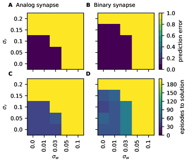
To study how the variability influences the prediction performance, we assess the prediction error and episodes-to-solution for different magnitudes of the read and write variability and , respectively. Both networks with either analog or binary synapses allow similar read and write noise levels, with the binary synapse being slightly more resilient toward the read noise (fig. 11A,B). In both cases, the write noise is more detrimental as it accumulates across the different learning episodes and can therefore have a higher impact on the learning performance. The read noise tends to average out as it is independent across the learning episodes. Overall, increasing the read or write variability beyond what is acceptable leads to a spurious activation of the dAPs, i.e., predictions, and a decline in the prediction performance. Concerning the learning speed, the number of episodes-to-solution is similar for the different variability levels where the learning is successful (fig. 11C,D).
2.3.4 Robustness of the model against synaptic failure
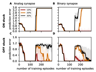
When operating ReRAM devices, they risk failing by getting trapped in the HCS even after applying voltage pulses with the appropriate magnitude across them (Kumar et al., 2017). To study how synaptic failure affects the prediction performance, we first train the network till it reaches zero prediction error (after episodes in fig. 12). Then, the conductance of a random fraction of synapses is set to the HCS. We quantify the level of synaptic failure by the ratio between the number of failed synapses and the total number of existing synapses. In the spiking TM model, a neuron may falsely generate a dAP if a sufficient number of its synapses are randomly switched to the HCS (this number can be approximated as the ratio , where is the dAP threshold and is the maximum conductance). This may result in generating false positives and thus an increase in the prediction error. This is confirmed by our results presented in fig. 12A,B. At up to synaptic failure no impact is observed on the prediction performance (fig. 12A,B). At greater than synaptic failure the performance of the network declines and does not recover.
In a second experiment, instead of turning a selection of random synapses to the HCS, we turn them to the LCS. For the different levels of synaptic failures, the performance of the network initially declines. Due to the failing synapses, which are stuck at the LCS, the neurons in certain subpopulations do not receive enough current and are thus not able to generate dAPs, i.e., make predictions. After further training episodes, the prediction errors converge back to zero as the network relearns using other synapses (fig. 12C,D). At greater than synaptic failure the performance does not recover due to the absence of alternative connections to form sequence-specific pathways.
3 Discussion
3.1 Summary
In this work, we demonstrate that the learning rules of the spiking temporal memory (spiking TM) model proposed by Bouhadjar et al. (2022b) can be realized using memristive dynamics. We investigate this for a particular type of memristive device known as VCM ReRAM (Waser, 2012a). To this end, we show that the spiking TM retains high prediction performance for a broad range of on-off ratios and learning rates. The model is resilient toward the write and read variability as well as the dependence of the synaptic updates on the weight. Moreover, our results show that the VCM-type ReRAM device can be operated either in the binary or the gradual switching regime without performance loss. This is in line with the original spiking TM implementation, which shows that the learning rule can either be implemented using structural plasticity where the weight abruptly changes between two levels or a conventional form of STDP where the weight gradually changes until it saturates. This suggests that the intrinsic dynamics of the VCM ReRAM capture not only synaptic properties of biological synapses such as the variability and the dependence of the synaptic updates on the weight but also can implement known forms of plasticity in the neuroscientific literature. Our study, therefore, ties further principles from the biological and the memristive synapses.
3.2 Relationship to previous models
In artificial neural networks trained by gradient-based approaches, ReRAM nonidealities can severely undermine the overall performance (Fouda et al., 2020). Due to the ReRAM variability, devices can be hardly programmed to a desired state, and the asymmetry in the conductance change can affect the propagation of the gradient and lead to performance loss. Correcting for these nonidealities can be costly and may require additional circuitry (Chen et al., 2015; Agarwal et al., 2016; Hong et al., 2018; Yu, 2018; Ambrogio et al., 2018; Adnan et al., 2021). We know that biological neuronal networks carry out accurate computations despite their synaptic nonideal characteristics such as variability. This suggests the existence of biological principles accommodating that, which we need to understand and port to successfully implement neuromorphic hardware. The spiking TM and other brain-inspired self-organizing networks (Lazar et al., 2009; Yi et al., 2022) suggest a set of biological concepts that might be at the heart of brain processing capabilities. For instance, the highly sparse connectivity and activity of the spiking TM are observed in biological networks, and they are essential for increasing the capacity of the system and decreasing energy consumption.
There are a number of biologically motivated sequence learning models that are closely related to the spiking TM, such as the self-organizing recurrent neural network model (SORN, Lazar et al., 2009). Recent work incorporated memristive dynamics into the synapses and neurons of the SORN model and showed that it retains successful performance (Payvand et al., 2022). The authors studied the role of variability and showed that it can improve prediction performance. However, the other memristive nonidealities were not studied systematically. It remains also to be investigated whether the model can learn high-order sequences similar to the ones presented in our work.
3.3 Outlook
Neuromorphic hardware that relies on components implemented in the analog domain is noisy and heterogeneous, similar to real brains (Zhu et al., 2020). To date, there are only speculations on how the brain contributes to sensible and reliable behavior in the face of these imperfections. By using neuromorphic hardware as a test substrate, we expect to gain new insights into the neural principles that solve this issue. In this study, it was apparent that ReRAM devices share the same characteristics as biological synapses including the weight dependence of the synaptic updates, limited dynamics range, and variability. Throughout the work on these neuromorphic systems, we can develop intuitions of how the biological synapse exploits these different characteristics. For instance, similar to biological synapses, ReRAM devices are characterized by a read and write variability. In the biological system, the read variability is analogous to the randomness in the vesicle release, and the write variability corresponds to the randomness in the density regulation of the postsynaptic receptors. So far, it is not clear how these different characteristics contribute to the learning dynamics in the biological system. Neuromorphic hardware can provide an environment where this question can be studied.
In this work, we show that the model is resilient toward synaptic variability. Other works show that synaptic variability can even have a computational benefit (Dalgaty et al., 2021). For example, in probabilistic computing frameworks, the variability is considered a prerequisite for efficient probabilistic inference (Buesing et al., 2011; Suri et al., 2013; Maass, 2014; Neftci et al., 2016; Dutta et al., 2022). It allows the system to explore the state space and come up with an estimate of how likely is each solution. Similarly, a recent extension of the spiking TM model shows that the model can learn to replay probabilistic sequences using noise (Bouhadjar et al., 2022a). The study however explored only correlated additive noise. Future work can shed light on the possibility of using ReRAM noise, i.e., multiplicative noise, as an alternative.
Ultimately, the goal is to implement the spiking TM model on a standalone neuromorphic chip. In this work, we only investigate how the intrinsic properties of the memristive device affect the learning in the spiking TM. In a concurrent study, we devise a complete design of the neuromorphic circuit implementing the different components of the spiking TM (Siegel et al., 2022) and showed in simulations that the system supports successful prediction performance. A future study needs to verify these design principles in physical electronic circuits.
4 Conclusion
A prerequisite for the success of analog neuromorphic hardware is the identification of hardware devices that can best implement neuroscientific mechanisms and concepts. ReRAM devices were suggested as promising synaptic elements due to their scalability and energy efficiency. In this work, we identified that both analog and binary types of ReRAM device can be used to implement well-known plasticity models from the neuroscientific literature and demonstrated their suitability as synaptic elements in the biologically inspired spiking TM model.
5 Methods
In the following summarizing tables (table 1), we provide an overview of the network model, the training protocol, and the simulation details. Parameter values can be found in table 2. See (Bouhadjar et al., 2022b) for a detailed description of the model.
5.1 Model tables
| Summary | |
|---|---|
| Populations | excitatory neurons (), inhibitory neurons (), external spike sources (); and composed of disjoint subpopulations and () |
| Connectivity | • sparse random connectivity between excitatory neurons (plastic) • local recurrent connectivity between excitatory and inhibitory neurons (static) |
| Neuron model | • excitatory neurons: leaky integrate-and-fire (LIF) with nonlinear input integration (dendritic action potentials) • inhibitory neurons: leaky integrate-and-fire (LIF) |
| Synapse model | exponential postsynaptic currents (PSCs) |
| Plasticity | homeostatic spike-timing dependent plasticity in excitatory-to-excitatory connections |
| Populations | ||
|---|---|---|
| Name | Elements | Size |
| excitatory (E) neurons | ||
| inhibitory (I) neurons | ||
| excitatory neurons in subpopulation , | ||
| inhibitory neurons in subpopulation , | ||
| external spike sources | ||
| Connectivity | ||
|---|---|---|
| Source population | Target population | Pattern |
| random; fixed in-degrees , delays , synaptic time constants plastic weights (; “EE connections”) | ||
| all-to-all; fixed delays , synaptic time constants , and weights (; “IE connections”) | ||
| all-to-all; fixed delays , synaptic time constants , and weights (; “EI connections”) | ||
| none (; “II connections”) | ||
| one-to-all; fixed delays , synaptic time constants , and weights (; “EX connections”) | ||
| no self-connections (“autapses”), no multiple connections (“multapses”) | ||
| all unmentioned connections , , , () are absent | ||
| Neuron and synapse | |
| Neuron | |
| Type | leaky integrate-and-fire (LIF) dynamics |
| Description | dynamics of membrane potential of neuron : • emission of the th spike of neuron at time if (7) with somatic spike threshold • reset and refractoriness: with refractory time and reset potential • subthreshold dynamics: (8) with membrane resistance , membrane time constant , and total synaptic input current • , , , () • , , , () |
| Synapse | |
| Type | exponential or alpha-shaped postsynaptic currents (PSCs) |
| Description | • total synaptic input current (9) (9) with dendritic, inhibitory, external and excitatory input currents , , , evolving according to (10) with and (11) (12) (13) with , , and synaptic time constants of EX, EI, and IE connections, respectively, the synaptic weight, and the read voltage • presynaptic spike trains • dAP generation: – emission of th dAP of neuron at time if – dAP current plateau: (14) with dAP current plateau amplitude , dAP current duration , and dAP activation threshold . |
| Plasticity | |
|---|---|
| Type | Hebbian-type plasticity and dAP-rate homeostasis |
| EE synapses | • Hebbian plasticity described in section 2.1 • homeostatic control: – if : a depression pulse is applied (see eq. 1 or eq. 3) – if : a potentiation pulse is applied (see eq. 1 or eq. 3) with the dAP trace and target dAP activity . • dAP trace of postsynaptic neuron , evolving according to with onset time of the th dAP, homeostasis time constant |
| all other synapses | non-plastic |
| Input |
| • repetitive stimulation of the network using the same set of sequences of ordered discrete items with number of sequences and length of th sequence • presentation of sequence element at time modeled by a single spike generated by the corresponding external source • inter-stimulus interval between subsequent sequence elements and within a sequence • inter-sequence time interval between subsequent sequences and • example sequence sets: – sequence set: ={, , , } |
| Output |
| • somatic spike times • dendritic currents () |
| Initial conditions and network realizations |
| • membrane potentials: () • dendritic currents: () • external currents: () • inhibitory currents: () • excitatory currents: () • synaptic permanences: with () • synaptic weights: with () (analog synapse) • synaptic weights: () (binary synapse) • spike traces: () • dAP traces: () • potential connectivity and initial permanences randomly and independently drawn for each network realization |
| Simulation details |
| • network simulations performed in NEST (Gewaltig and Diesmann, 2007) version 3.0 (Hahne et al., 2021) • definition of excitatory neuron model using NESTML (Plotnikov et al., 2016; Nagendra Babu et al., 2021) • synchronous update using exact integration of system dynamics on discrete-time grid with step size (Rotter and Diesmann, 1999) |
5.2 Model and simulation parameters
| Name | Value | Description |
| Network | ||
| total number of excitatory neurons | ||
| total number of inhibitory neurons | ||
| number of excitatory subpopulations (= number of external spike sources) | ||
| number of excitatory neurons per subpopulation | ||
| number of inhibitory neurons per subpopulation | ||
| (target) number of active neurons per subpopulation after learning = minimal number of coincident excitatory inputs required to trigger a spike in postsynaptic inhibitory neurons | ||
| (Potential) Connectivity | ||
| number of excitatory inputs per excitatory neuron (EE in-degree) | ||
| probability of potential (excitatory) connections | ||
| number of inhibitory inputs per excitatory neuron (EI in-degree) | ||
| number of excitatory inputs per inhibitory neuron (IE in-degree) | ||
| number of inhibitory inputs per inhibitory neuron (II in-degree) | ||
| Excitatory neurons | ||
| membrane time constant | ||
| absolute refractory period | ||
| membrane capacity | ||
| reset potential | ||
| somatic spike threshold | ||
| dAP current plateau amplitude | ||
| dAP duration | ||
| see eq. 6 | dAP threshold | |
| Inhibitory neurons | ||
| membrane time constant | ||
| absolute refractory period | ||
| membrane capacity | ||
| reset potential | ||
| spike threshold | ||
| Name | Value | Description |
| Synapse | ||
| weight of IE connections (EPSP amplitude) | ||
| weight of IE connections (EPSC amplitude) | ||
| weight of EI connections (IPSP amplitude) | ||
| weight of EI connections (IPSC amplitude) | ||
| weight of EX connections (EPSP amplitude) | ||
| weight of EX connections (EPSC amplitude) | ||
| synaptic time constant of EE connections | ||
| synaptic time constant of IE connections | ||
| synaptic time constant of EI connections | ||
| synaptic time constant of EX connection | ||
| delay of EE connections (dendritic) | ||
| delay of IE connections | ||
| delay of EI connections | ||
| delay of EX connections | ||
| Plasticity | ||
|
(analog synapse),
(binary synapse) |
potentiation learning rate | |
| depression rate | ||
| ratio between depression and potentiation learning rates | ||
| homeostasis rate | ||
| weight dependence (potentiation) exponent (default parameter) | ||
| weight dependence (depression) exponent (default parameter) | ||
| synapse maturity threshold | ||
| minimum permanence | ||
| minimum conductance | ||
| maximum conductance | ||
| minimal initial conductance | ||
| maximal initial conductance | ||
| maximal initial permanence | ||
| minimal initial permanence | ||
| maximal initial permanence | ||
| read noise | ||
| write noise | ||
| target dAP activity | ||
| homeostasis time constant | ||
| Input | ||
| number of sequences per set | ||
| number of characters per sequence | ||
| alphabet length | ||
| inter-stimulus interval | ||
| inter-sequence interval | ||
| Simulation | ||
| time resolution | ||
| number of training episodes | ||
Acknowledgments
This project was funded by the Helmholtz Association Initiative and Networking Fund (project number SO-092, Advanced Computing Architectures), and the European Union’s Horizon 2020 Framework Programme for Research and Innovation under the Specific Grant Agreement No. 785907 (Human Brain Project SGA2) and No. 945539 (Human Brain Project SGA3). Open access publication was funded by the Deutsche Forschungsgemeinschaft (DFG, German Research Foundation; grant 491111487).
Author contributions
All authors conceived and designed the work. YB performed the simulations and analyzed and visualized the data. YB wrote the first draft of the manuscript. All authors reviewed the manuscript and approved it for publication. YB was supervised by TT and DJW.
References
- Adnan et al. (2021) Adnan, M. M., S. Sayyaparaju, S. D. Brown, M. S. A. Shawkat, C. D. Schuman, and G. S. Rose (2021). Design of a robust memristive spiking neuromorphic system with unsupervised learning in hardware. ACM Journal on Emerging Technologies in Computing Systems 17(4), 1–26.
- Agarwal et al. (2016) Agarwal, S., S. J. Plimpton, D. R. Hughart, A. H. Hsia, I. Richter, J. A. Cox, C. D. James, and M. J. Marinella (2016). Resistive memory device requirements for a neural algorithm accelerator. In 2016 International Joint Conference on Neural Networks (IJCNN). IEEE.
- Ambrogio et al. (2018) Ambrogio, S., P. Narayanan, H. Tsai, R. M. Shelby, I. Boybat, C. di Nolfo, S. Sidler, M. Giordano, M. Bodini, N. C. P. Farinha, B. Killeen, C. Cheng, Y. Jaoudi, and G. W. Burr (2018). Equivalent-accuracy accelerated neural-network training using analogue memory. Nature 558(7708), 60–67.
- Bengel et al. (2020) Bengel, C., A. Siemon, F. Cuppers, S. Hoffmann-Eifert, A. Hardtdegen, M. von Witzleben, L. Hellmich, R. Waser, and S. Menzel (2020). Variability-aware modeling of filamentary oxide-based bipolar resistive switching cells using SPICE level compact models. IEEE Transactions on Circuits and Systems I: Regular Papers 67(12), 4618–4630.
- Bouhadjar et al. (2019) Bouhadjar, Y., M. Diesmann, R. Waser, D. J. Wouters, and T. Tetzlaff (2019). Constraints on sequence processing speed in biological neuronal networks. In Proceedings of the International Conference on Neuromorphic Systems, pp. 1–9.
- Bouhadjar et al. (2022a) Bouhadjar, Y., D. J. Wouters, M. Diesmann, and T. Tetzlaff (2022a). Coherent noise enables probabilistic sequence replay in spiking neuronal networks. ArXiv, 2206.10538.
- Bouhadjar et al. (2022b) Bouhadjar, Y., D. J. Wouters, M. Diesmann, and T. Tetzlaff (2022b). Sequence learning, prediction, and replay in networks of spiking neurons. PLOS Computational Biology 18(6), e1010233.
- Buesing et al. (2011) Buesing, L., J. Bill, B. Nessler, and W. Maass (2011). Neural dynamics as sampling: A model for stochastic computation in recurrent networks of spiking neurons. PLOS Computational Biology 7, e1002211.
- Burr et al. (2016) Burr, G. W., R. M. Shelby, A. Sebastian, S. Kim, S. Kim, S. Sidler, K. Virwani, M. Ishii, P. Narayanan, A. Fumarola, L. L. Sanches, I. Boybat, M. L. Gallo, K. Moon, J. Woo, H. Hwang, and Y. Leblebici (2016). Neuromorphic computing using non-volatile memory. Advances in Physics: X 2(1), 89–124.
- Chen et al. (2015) Chen, P.-Y., B. Lin, I.-T. Wang, T.-H. Hou, J. Ye, S. Vrudhula, J. sun Seo, Y. Cao, and S. Yu (2015). Mitigating effects of non-ideal synaptic device characteristics for on-chip learning. In 2015 IEEE/ACM International Conference on Computer-Aided Design (ICCAD). IEEE.
- Cüppers et al. (2019) Cüppers, F., S. Menzel, C. Bengel, A. Hardtdegen, M. von Witzleben, U. Böttger, R. Waser, and S. Hoffmann-Eifert (2019). Exploiting the switching dynamics of HfO2-based ReRAM devices for reliable analog memristive behavior. APL Materials 7(9), 091105.
- Dalgaty et al. (2021) Dalgaty, T., N. Castellani, C. Turck, K.-E. Harabi, D. Querlioz, and E. Vianello (2021). In situ learning using intrinsic memristor variability via markov chain monte carlo sampling. Nature Electronics 4(2), 151–161.
- Dittmann and Strachan (2019) Dittmann, R. and J. P. Strachan (2019). Redox-based memristive devices for new computing paradigm. APL Materials 7(11), 110903.
- Doevenspeck et al. (2018) Doevenspeck, J., R. Degraeve, A. Fantini, P. Debacker, D. Verkest, R. Lauwereins, and W. Dehaene (2018). Temporal sequence learning with a history-sensitive probabilistic learning rule intrinsic to oxygen vacancy-based rram. In 2018 IEEE International Electron Devices Meeting (IEDM), pp. 20–5. IEEE.
- Dutta et al. (2022) Dutta, S., G. Detorakis, A. Khanna, B. Grisafe, E. Neftci, and S. Datta (2022). Neural sampling machine with stochastic synapse allows brain-like learning and inference. Nature Communications 13(1), 2571.
- Fantini et al. (2013) Fantini, A., L. Goux, R. Degraeve, D. Wouters, N. Raghavan, G. Kar, A. Belmonte, Y.-Y. Chen, B. Govoreanu, and M. Jurczak (2013). Intrinsic switching variability in HfO 2 RRAM. In 2013 5th IEEE International Memory Workshop, pp. 30–33. IEEE.
- Fleck et al. (2016) Fleck, K., C. La Torre, N. Aslam, S. Hoffmann-Eifert, U. Böttger, and S. Menzel (2016). Uniting gradual and abrupt set processes in resistive switching oxides. Physical review applied 6(6), 064015.
- Fouda et al. (2020) Fouda, M. E., F. Kurdahi, A. Eltawil, and E. Neftci (2020). Spiking neural networks for inference and learning: a memristor-based design perspective. In S. Spiga, A. Sebastian, D. Querlioz, and B. Rajendran (Eds.), Memristive Devices for Brain-Inspired Computing, Woodhead Publishing Series in Electronic and Optical Materials, pp. 499–530. Woodhead Publishing.
- Fusi and Abbott (2007) Fusi, S. and L. F. Abbott (2007). Limits on the memory storage capacity of bounded synapses. Nature Neuroscience 10(4), 485–493.
- Gewaltig and Diesmann (2007) Gewaltig, M.-O. and M. Diesmann (2007). NEST (NEural Simulation Tool). Scholarpedia Journal 2(4), 1430.
- Hahne et al. (2021) Hahne, J., S. Diaz, A. Patronis, W. Schenck, A. Peyser, S. Graber, S. Spreizer, S. B. Vennemo, T. Ippen, H. Mørk, J. Jordan, J. Senk, S. Konradi, P. Weidel, T. Fardet, D. Dahmen, D. Terhorst, J. Stapmanns, G. Trensch, A. van Meegen, J. Pronold, J. M. Eppler, C. Linssen, A. Morrison, A. Sinha, J. Mitchell, S. Kunkel, R. Deepu, E. Hagen, T. Vierjahn, N. L. Kamiji, R. de Schepper, P. Machado, J. Albers, W. Klijn, A. Myczko, W. Mayner, P. Nagendra Babu, H. Jiang, S. Billaudelle, B. S. Vogler, G. Miotto, L. Kusch, A. Antonietti, A. Morales-Gregorio, J. Dolderer, Y. Bouhadjar, and H. E. Plesser (2021). Nest 3.0.
- Hardtdegen et al. (2018) Hardtdegen, A., C. L. Torre, F. Cuppers, S. Menzel, R. Waser, and S. Hoffmann-Eifert (2018). Improved switching stability and the effect of an internal series resistor in HfO 2/TiO x bilayer ReRAM cells. IEEE Transactions on Electron Devices 65(8), 3229–3236.
- Hawkins and Ahmad (2016) Hawkins, J. and S. Ahmad (2016). Why neurons have thousands of synapses, a theory of sequence memory in neocortex. Frontiers in Neural Circuits 10, 23.
- Hong et al. (2018) Hong, X., D. J. Loy, P. A. Dananjaya, F. Tan, C. Ng, and W. Lew (2018). Oxide-based RRAM materials for neuromorphic computing. Journal of Materials Science 53(12), 8720–8746.
- Ielmini and Wong (2018) Ielmini, D. and H.-S. P. Wong (2018). In-memory computing with resistive switching devices. Nature Electronics 1(6), 333–343.
- Jordan et al. (2018) Jordan, J., T. Ippen, M. Helias, I. Kitayama, M. Sato, J. Igarashi, M. Diesmann, and S. Kunkel (2018). Extremely scalable spiking neuronal network simulation code: From laptops to exascale computers. Frontiers in Neuroinformatics 12, 2.
- Kumar et al. (2017) Kumar, S., Z. Wang, X. Huang, N. Kumari, N. Davila, J. P. Strachan, D. Vine, A. L. D. Kilcoyne, Y. Nishi, and R. S. Williams (2017). Oxygen migration during resistance switching and failure of hafnium oxide memristors. Applied Physics Letters 110(10), 103503.
- Kunkel et al. (2014) Kunkel, S., M. Schmidt, J. M. Eppler, G. Masumoto, J. Igarashi, S. Ishii, T. Fukai, A. Morrison, M. Diesmann, and M. Helias (2014). Spiking network simulation code for petascale computers. Frontiers in Neuroinformatics 8, 78.
- Lazar et al. (2009) Lazar, A., G. Pipa, and J. Triesch (2009). SORN: a self-organizing recurrent neural network. Frontiers in Computational Neuroscience 3, 23.
- Maass (2014) Maass, W. (2014). Noise as a resource for computation and learning in networks of spiking neurons. Procedings of the IEEE 102(5), 860–880.
- Marković et al. (2020) Marković, D., A. Mizrahi, D. Querlioz, and J. Grollier (2020). Physics for neuromorphic computing. Nature Reviews Physics 2(9), 499–510.
- Masquelier and Thorpe (2007) Masquelier, T. and S. J. Thorpe (2007). Unsupervised learning of visual features through spike timing dependent plasticity. PLOS Computational Biology 3(2), e31.
- Nagendra Babu et al. (2021) Nagendra Babu, P., C. Linssen, J. M. Eppler, T. Schulte to Brinke, A. Ziaeemehr, T. Fardet, Y. Bouhadjar, R. Duarte, B. Rumpe, and A. Morrison (2021). Nestml 4.0.
- Neftci and Averbeck (2019) Neftci, E. O. and B. B. Averbeck (2019). Reinforcement learning in artificial and biological systems. Nature Machine Intelligence 1(3), 133–143.
- Neftci et al. (2016) Neftci, E. O., B. U. Pedroni, S. Joshi, M. Al-Shedivat, and G. Cauwenberghs (2016). Stochastic synapses enable efficient brain-inspired learning machines. Frontiers in Neuroscience 10, 241.
- Payeur et al. (2021) Payeur, A., J. Guerguiev, F. Zenke, B. A. Richards, and R. Naud (2021). Burst-dependent synaptic plasticity can coordinate learning in hierarchical circuits. Nature Neuroscience 24(7), 1010–1019.
- Payvand et al. (2022) Payvand, M., F. Moro, K. Nomura, T. Dalgaty, E. Vianello, Y. Nishi, and G. Indiveri (2022). Self-organization of an inhomogeneous memristive hardware for sequence learning. Nature Communications 13(1), 5793.
- Plotnikov et al. (2016) Plotnikov, D., I. Blundell, T. Ippen, J. M. Eppler, B. Rumpe, and A. Morrison (2016). NESTML: a modeling language for spiking neurons. In A. Oberweis and R. Reussner (Eds.), Modellierung 2016, Volume P-254 of Lecture Notes in Informatics (LNI), pp. 93–108. Modellierung 2016, Karlsruhe (Germany), 17 Mar 2016 - 19 Mar 2016: Gesellschaft für Informatik e.V. (GI).
- Rotter and Diesmann (1999) Rotter, S. and M. Diesmann (1999). Exact digital simulation of time-invariant linear systems with applications to neuronal modeling. Biological Cybernetics 81(5-6), 381–402.
- Siegel et al. (2022) Siegel, S., Y. Bouhadjar, T. Tetzlaff, R. Waser, R. Dittmann, and D. J. Wouters (2022). Neuromorphic sequence learning on a memristive crossbar array (in preparation).
- Suri et al. (2013) Suri, M., D. Querlioz, O. Bichler, G. Palma, E. Vianello, D. Vuillaume, C. Gamrat, and B. DeSalvo (2013). Bio-inspired stochastic computing using binary CBRAM synapses. IEEE Transactions on Electron Devices 60(7), 2402–2409.
- Wang et al. (2015) Wang, Z., S. Ambrogio, S. Balatti, and D. Ielmini (2015). A 2-transistor/1-resistor artificial synapse capable of communication and stochastic learning in neuromorphic systems. Frontiers in Neuroscience 8, 438.
- Waser (2012a) Waser, R. (2012a). Nanoelectronics and information technology: advanced electronic materials and novel devices. John Wiley & Sons.
- Waser (2012b) Waser, R. (2012b). Redox-based resistive switching memories. Journal of Nanoscience and Nanotechnology 12(10), 7628–7640.
- Waser et al. (2009) Waser, R., R. Dittmann, G. Staikov, and K. Szot (2009). Redox-based resistive switching memories - nanoionic mechanisms, prospects, and challenges. Advanced Materials 21(25-26), 2632–2663.
- Xia and Yang (2019) Xia, Q. and J. J. Yang (2019). Memristive crossbar arrays for brain-inspired computing. Nature Materials 18(4), 309–323.
- Yang et al. (2013) Yang, J. J., D. B. Strukov, and D. R. Stewart (2013). Memristive devices for computing. Nature nanotechnology 8(1), 13–24.
- Yi et al. (2022) Yi, S., J. D. Kendall, R. S. Williams, and S. Kumar (2022). Activity-difference training of deep neural networks using memristor crossbars. Nature Electronics, s41928–022–00869–w.
- Yu (2018) Yu, S. (2018). Neuro-inspired computing with emerging nonvolatile memorys. Procedings of the IEEE 106(2), 260–285.
- Zamarreño-Ramos et al. (2011) Zamarreño-Ramos, C., L. A. Camuñas-Mesa, J. A. Pérez-Carrasco, T. Masquelier, T. Serrano-Gotarredona, and B. Linares-Barranco (2011). On spike-timing-dependent-plasticity, memristive devices, and building a self-learning visual cortex. Frontiers in Neuroscience 5, 26.
- Zhao et al. (2020) Zhao, M., B. Gao, J. Tang, H. Qian, and H. Wu (2020). Reliability of analog resistive switching memory for neuromorphic computing. Applied Physics Reviews 7(1), 011301.
- Zhao et al. (2019) Zhao, Y., W. Shen, P. Huang, W. Xu, M. Fan, X. Liu, and J. Kang (2019). A physics-based model of RRAM probabilistic switching for generating stable and accurate stochastic bit-streams. In 2019 IEEE International Electron Devices Meeting (IEDM). IEEE.
- Zhu et al. (2020) Zhu, J., T. Zhang, Y. Yang, and R. Huang (2020). A comprehensive review on emerging artificial neuromorphic devices. Applied Physics Reviews 7(1), 011312.
Appendix A Supporting information
