Rigorous Assessment of Model Inference Accuracy using Language Cardinality
Abstract.
Models such as finite state automata are widely used to abstract the behavior of software systems by capturing the sequences of events observable during their execution. Nevertheless, models rarely exist in practice and, when they do, get easily outdated; moreover, manually building and maintaining models is costly and error-prone. As a result, a variety of model inference methods that automatically construct models from execution traces have been proposed to address these issues.
However, performing a systematic and reliable accuracy assessment of inferred models remains an open problem. Even when a reference model is given, most existing model accuracy assessment methods may return misleading and biased results. This is mainly due to their reliance on statistical estimators over a finite number of randomly generated traces, introducing avoidable uncertainty about the estimation and being sensitive to the parameters of the random trace generative process.
This paper addresses this problem by developing a systematic approach based on analytic combinatorics that minimizes bias and uncertainty in model accuracy assessment by replacing statistical estimation with deterministic accuracy measures. We experimentally demonstrate the consistency and applicability of our approach by assessing the accuracy of models inferred by state-of-the-art inference tools against reference models from established specification mining benchmarks.
1. Introduction
Software system models, typically in the form of Finite State Automata (FSA), have been widely used to abstract the behavior of software components and their interactions. Such models are important in many applications, including test data generation (Fraser and Walkinshaw, 2012), model checking (Clarke Jr et al., 2018), and program comprehension (Cook and Wolf, 1998). Nevertheless, they are rarely available during software development and, if they do, get easily outdated. This is mainly because manually building and maintaining such models is both time-consuming and error-prone. To address this problem, a variety of model inference algorithms have been proposed (Biermann and Feldman, 1972; Beschastnikh et al., 2011; Walkinshaw et al., 2016; Emam and Miller, 2018; Mariani et al., 2017). These algorithms automatically extract a system’s behavior model by capturing visible events generated during the system’s execution.
Model assessment, i.e., assessing the accuracy of inferred models, is an essential task to evaluate and compare different model inference algorithms. When reference models are given as ground truth, model assessment seems straightforward; for example, one can compute the similarity between the languages defined by the inferred and reference models. However, the languages are often infinite, making it complex to measure the degree of their similarity.
To address this issue, it is common to rely on statistical accuracy estimation. For example, the idea behind a popular method, called trace similarity (Lo and Khoo, 2006a), is to generate sampled traces111A trace is the sequence of events generated during the system’s execution. Also known as run, sequence, execution trace. by randomly traversing both reference and inferred models, and estimate the accuracy by checking how many of the traces generated using one model are accepted by the other. The idea is that a high number of accepted sampled traces is an indicator of a high degree of similarity. Although this idea is very intuitive, the random traverse can introduce a large degree of uncertainty about the estimation, depending on the parameters of the random trace generative process (e.g., the probability of ending the traverse in an accepting state rather than continuing through one of its outgoing transitions), and the topology of the model (e.g., a model may have features that are hard to exercise through random exploration). While there is no intrinsic probability distribution over the traces accepted by a finite state model, the random trace generation does induce such a distribution, therefore introducing an evaluation bias: the measured accuracy will reflect how well the inferred model can classify traces drawn according to that distribution.
In an attempt to reduce the uncertainty due to the random traversal, an alternative consists in using deterministic trace generation methods (Walkinshaw et al., 2008). These generate sets of traces that are guaranteed to cover all the models’ behaviors without favoring any specific one. Although this increases the reproducibility and the chances of revealing discrepancies, there are still remaining issues. First, each discrepancy (a trace upon which the reference and the inferred model disagree) may be representative of a larger or smaller class of traces, thus making it difficult to quantify its impact. Second, these methods often generate sets of traces containing a disproportionately large amount of traces not accepted by the reference model, which may lead to skewed accuracy results. Third, the generated set of traces can become exceedingly large if the difference between the number of states in the reference and the inferred model is large, which is a common occurrence in model inference, hindering its practical usability.
In this paper we propose a method to rigorously measure the accuracy of an inferred model against a reference one (both in the form of FSA) by considering all the possible traces up to an arbitrary finite maximum trace length. The maximum trace length considered is a parameter set by the user, which can be set to a value relevant for the application under analysis, to a value large enough to guarantee that all the behaviors of the reference and inferred models are exercised, or to an arbitrarily large value, effectively computing the asymptotic accuracy.
Our method is deterministic (i.e., for a given pair of reference and inferred models it always returns the same result), does not depend on the model structure (i.e., assessing against the same reference model different models accepting the same language will generate the same accuracy measurement), and does not introduce any evaluation bias other than the maximum trace length (i.e., the computed metrics accurately describe how well the inferred model can classify traces drawn with uniform distribution from the set of all the traces up to the maximum length).
Within this paper we also highlight how an inferred model can show a variable level of accuracy depending on the length of the traces used in the assessment. This is an aspect that is generally not considered by current assessment methodologies. Following this observation, we propose an additional assessment method that computes a pair of precision and recall values for each trace length, within a range specified by the user. Each value considers all the possible traces of a given length.
Central to our solution is the use of analytic combinatorics to count the number of traces in a (possibly infinite) regular language, up to an arbitrary maximum trace length, without explicitly enumerating them. In this regard, to increase the practical applicability of our approach, we improved the scalability of the analytic combinatorics approaches currently used to compute the cardinality of regular languages (Flajolet and Sedgewick, 2009).
We have implemented the proposed method in a prototype and experimentally evaluated it using reference models previously used in the model inference literature, and inferred models generated using well known model inference methods. The experimental results obtained when assessing the applicability of our method on the real-world model show that it is scalable enough to be used in practice. We have also compared the generated accuracy measurements with the results obtained using other popular assessment methods. The results indicate differences caused by the evaluation bias introduced by current assessment methods, and show that our proposed approach can be used to address this issue.
Significance
Assessing the accuracy of inferred models against ground truth reference models is crucial in evaluating newly developed model inference methods, as it serves as the primary method for evaluating effectiveness and comparing different inference techniques. Our work is targeting researchers involved in the development or evaluation of model inference methods. Our goal is to provide a tool to evaluate inference algorithms, rather than the inferred models. In particular, we highlight how currently commonly used assessment methods can generate misleading results, thus interfering with the development of effective inference techniques and creating false expectations about the quality of the inferred models. Furthermore, through our novel model assessment method, we provide more accurate and comprehensive insights about the model assessment results, including new insights describing how the model accuracy differs when evaluating it on traces of different lengths.
Contributions
In summary, this paper makes the following contributions:
-
•
A novel model assessment method that measures the precision and recall values of an inferred model, with respect to a reference ground truth model, considering all the traces up to a finite maximum trace length. This method is:
-
–
Deterministic: repeated executions return the same result.
-
–
Comprehensive: it considers all the traces up to the maximum length.
-
–
Unbiased: all the traces considered in the evaluation have the same weight on the result.
-
–
Model-independent: assessing different models accepting the same language against the same reference model generates the same result.
-
–
-
•
A further development of the assessment method, measuring the model accuracy separately for each trace length, over a given range.
-
•
An empirical comparison of the accuracy measurement obtained using our methods with measurements generated using other popular assessment methods.
-
•
An experimental evaluation of the applicability of our method.
-
•
An improvement of currently used analytic combinatorics approaches to compute the cardinality of regular languages, up to a finite maximum trace length.
Outline
The rest of the paper is organized as follows. In Section 2, we present a brief background on the theory of formal languages, model assessment, and analytic combinatorics as a tool to compute the cardinality of regular languages. In Section 3, we discuss two prominent classes of model assessment methods from the literature: statistical estimation (the most commonly used accuracy assessment method) and model-based (developed to address shortcomings of the first), reflecting on the open issues that motivated this work. Section 4 presents our main contribution: a novel assessment method, based on analytical measures for the cardinality of languages, that addresses the issues highlighted in the preceding section, and a further development that allows to evaluate how the model accuracy changes over a range of trace lengths. To increase the practical applicability of our method, in Section 5, we present an improvement of currently used analytic combinatorics approaches to compute the cardinality of regular languages. In Section 6 we evaluate our method experimentally, focusing on whether it is suitable to replace the assessment methods discussed in Section 3, and how the different methods’ assessment results compare. Section 7 presents relevant related work, and Section 8 concludes the paper with future work directions.
2. Background
2.1. Models and Languages
In this paper, we consider models in the form of Deterministic Finite-state Automata (DFA). A DFA is a tuple , where is a finite alphabet, is the set of states, is the initial state, is the set of accepting states, and is the transition function. A trace is a finite sequence of elements for . A trace is accepted by if there exists a sequence of states such that (1) for , (2) for , (3) is the initial state, and (4) . A state is an error state if no accepting state is reachable from . Let be the set of all possible traces over (including the empty trace). The language accepted by , denoted by , is the set of all traces accepted by . Two DFAs are equivalent if they accept the same language.
DFAs accept regular languages, which are closed under union, intersection, and complement. These operations on regular languages correspond to analogous operations on the automata accepting the languages. Therefore, with abuse of notation, we will use the union (), intersection (), and complement () operators on both automata and the languages they accept; for example, represents the DFA accepting any trace that is accepted by or not accepted by .
2.2. Model Assessment as Language Comparison
Given a reference model and an inferred model over the same alphabet , to assess the accuracy of the inferred model we need a measure of how well the language accepted by approximates the language accepted by . Drawing from established theory on classification assessment methods (Tharwat, 2020), can be partitioned into four subsets of traces: True Positives (), True Negatives (), False Positives (), and False Negatives ().
By generalization, any set of traces (which we call evaluation set) can be partitioned into four subsets , , , and , containing true positives, true negatives, false positives and false negatives, respectively. If the evaluation set is finite, several accuracy metrics can be defined based on the relative cardinality () of these four languages. In this paper, we will focus on precision and recall:
| (1) |
which are widely used in model inference literature (Krka et al., 2014; Lo et al., 2012; Lo and Khoo, 2006a).
It is worth noting that precision and recall cannot be used as distance functions in a metric space as they are not symmetric by definition. However, if needed, the model assessment approach discussed in this work can be adapted to compute the Jaccard distance (i.e., distance between and ) with respect to a finite evaluation set (bounded Jaccard), yielding a metric space.
In the rest of this paper we will continue to use and to denote the reference and the inferred model respectively, both assumed to be defined over the same alphabet .
2.3. Analytic Combinatorics and Cardinality of Regular Languages
Analytic combinatorics (Flajolet and Sedgewick, 2009) is a theory used to build, manipulate and analyze exact enumerative descriptions of combinatorial structures, typically focusing on structures whose realizations are too many for explicit enumeration. Generating functions are a core tool in analytic combinatorics, as they enable to concisely define and operate on certain infinite sequences. Let us consider a discrete, possibly infinite sequence of real values , with . An ordinary generating function (OGF) is a mathematical object encoding the sequence as the coefficients of a formal power series:
| (2) |
Given an OGF , the -th coefficient can be retrieved as the -th Taylor coefficient of
| (3) |
A regular language , accepted by a DFA , is a combinatorial structure representing all the traces belonging to the language. The sequence of cardinalities of is the sequence of number of traces of length accepted by , i.e., the cardinality of the language accepted by restricted to traces of length , . For our purpose, we aim at constructing an OGF denoted with encoding in a compact way the sequence of cardinalities of .
The OGF for the sequence of cardinalities of a regular language is always a rational function (Flajolet and Sedgewick, 2009). For example, let us consider the language , with . The empty trace, with length 0, is accepted (); two traces of length 1 are accepted (); four of length 2 (); and so on. The infinite sequence can be compactly encoded by the OGF .
Given a regular language , computing the OGF is typically reduced to the problem of counting the number of accepting paths of length of the minimal automaton accepting , via the established transfer matrix method (Flajolet and Sedgewick, 2009; Stanley, 2011). This algorithm relies on linear algebraic operations on the matrix representing the transition relation of the automaton (Flajolet and Sedgewick, 2009, Proposition I.3). While the transfer matrix method works in general, in Section 5 we will present an alternative, equivalent algorithm to obtain the OGF of a regular language that significantly outperformed the transfer matrix method in our tests.
Once the OGF has been computed using one of the above methods, the values of the sequence can be recovered as the Taylor coefficients of . Fortunately, since the OGF for the sequence of cardinalities of a regular language is always a rational function (Flajolet and Sedgewick, 2009) which can be written as the quotient between two finite degree polynomials , it is possible (and faster) to derive a recurrence relation that allows computing the values of the sequence without performing symbolic differentiation. Let and be polynomials of maximum degree , and recall that the OGF is equal to the formal power series with coefficients .
| (4) |
By multiplying by and expanding the sum, one obtains
| (5) |
and by equating the coefficients, (considering and equal to zero if ), one obtains and therefore which defines the sequence .
3. Existing methods for Model Assessment
Following Equation (1), when a finite evaluation set of traces is available, measuring the accuracy of against using precision and recall can be achieved by comparing the acceptance of each trace in . However, obtaining a finite and representative evaluation set over is a challenging problem. In this section, we discuss the two prominent classes of methods from the literature to generate evaluation sets for model assessment. Methods in the first class — Statistical Estimation — generate the evaluation set of traces by means of a random walk over the automata’s paths. Methods in the second class — Model-Based — use a deterministic traversal of the automata’s transition relation to generate an evaluation set that is likely to reveal divergences between the reference model and the inferred one.
3.1. Statistical Estimation using Random Walks
Statistical estimation (Busany et al., 2019; Lo et al., 2012, 2009; Walkinshaw and Bogdanov, 2013; Walkinshaw et al., 2013; Mariani et al., 2010) represents a class of model assessment methods based on finite evaluation multisets (denoted by ) of traces randomly generated (sampled) over . The random process used to generate is the characterizing element of each method. The most popular statistical estimation method is trace similarity, proposed by Lo and Khoo (2006a), which generates by performing random walks on the reference and inferred models, rather than generating random sequences from .
The core random walk algorithm is defined as follows, starting from the initial state. If the current state is accepting, the procedure randomly decides whether to terminate the walk or to continue; if the walk is not terminated, it randomly selects one among the outgoing transitions from the current state, adds the transition symbol to the trace, updates the current state to the target of the transition, and then the random walk continues from the new current state. If an error state222As defined in Section 2.1, an error state is a state from which no accepting state can be reached. is reached, the current trace is discarded and the random walk restarts from the initial state.
To compute the precision using trace similarity, an evaluation multiset is generated by performing random walks on the inferred model , therefore generating traces that are either true positives or false positives. Precision is then defined as the ratio of traces in accepted also by the reference model , i.e. the proportion of true positives333The rationale for this process stems from the observation that , which on the surface reminds of the conditional probability of a trace being accepted by given that the trace is accepted by . We shall demonstrate in the remaining of this section that this conditional probability interpretation is itself conditional on the random walk process, which may render the computed precision meaningless.. Similarly, to compute the recall, the evaluation multiset is generated by performing random walks on the reference model , generating traces that are either true positives or false negatives. Recall is then defined as the proportion of traces in accepted also by the inferred model . In both cases, model coverage can be achieved by repeated, independent random walks, e.g., until each transition is traversed a minimum number of times.
It is important to note that, when Lo and Khoo (2006a) originally proposed the trace similarity method, it was assumed either (a) that the models are probabilistic and the random walk is performed according to the transition probabilities of the models, or (b) that the models are deterministic and the user specifies how the random choices necessary to generate traces are made (defaulting to a uniform distribution over the outgoing transitions if not otherwise specified). The transition probability distribution is an important aspect of the assessment because, as we will soon discuss, it affects the results. In the model inference literature, the use of trace similarity on deterministic models, i.e., whose transition probabilities are not specified by the model itself, is predominant. This is because the inference methods that are most well-known (e.g., -tails (Biermann and Feldman, 1972)) or considered state-of-the-art (e.g., MINT (Walkinshaw et al., 2016)) generate deterministic models. Moreover, the reference models used in the assessment are also most often deterministic, because they are either manually created (for example, from API documentation and reference books (Pradel et al., 2010)) or they come from a formal specification of the target language, thus with no information about the probability distribution of the traces.
On the other hand, a random walk algorithm does require a probability distribution to select which transition to traverse at each step, and to decide whether to continue or to terminate the random walk when an accepting state is reached.
To decide which transition to follow, it is common practice to select one of the possible alternatives with uniform probability distribution (Lo and Khoo, 2006a). For the decision of whether to continue or terminate the random walk once a final state is reached, a number of strategies are commonly used; e.g., Walkinshaw et al. (2013) define a termination probability that is inversely proportional to the number of outgoing transitions.
A factor that is often overlooked in the statistical estimation of the model accuracy is how the (arbitrary) randomness of the trace generation impacts the model assessment. Inferred and reference models merely represent languages, i.e., (possibly infinite) sets of traces over a finite alphabet. There is no intrinsic probability distribution over the traces of a finite state model. On the other hand, the random trace generation process used to produce the evaluation multiset (e.g., a random walk, in the case of trace similarity) induces a probability distribution over the accepted language. This distribution may be non-uniform (i.e., different traces may be generated with different probabilities) therefore introducing a sampling bias in the model assessment: the precision and recall values obtained using this random sampling will reflect how well the inferred model can classify traces drawn according to that distribution. Unless this distribution reflects domain knowledge about the application being analyzed (i.e., if the models are purposefully probabilistic, and they describe the probability that different traces have of being generated by the system under analysis), this sampling bias is not desirable.
For example, let us consider a random walk using a fixed termination probability to decide the trace termination, and uniform sampling among the available alternatives to decide which transition to follow. Intuitively, the termination probability has an impact on the length of the sampled traces: increasing makes shorter traces more likely to be sampled (correspondingly, longer traces less likely). However, it is hard to predict the actual length distribution without taking into account the specific topology of the model from which the traces are sampled. Moreover, the topology of the model also induces a non-uniform distribution among accepted traces of the same length: the likelihood of a trace depends on the probability of selecting each of its transitions in a given order, with each of these selections generally depending on the number of successors of the source state.
We have thus identified two sampling biases in the random walk:
-
•
shorter traces are more likely to be sampled (but exactly how likely is topology-dependent);
-
•
for a given trace length, some traces are more likely to be sampled than others.
When a random walk is used to generate the evaluation multiset for trace similarity, both sampling biases become systematic faults of the method, and their impact on the model assessment is difficult to quantify a priori since both depend on specific random walk parameters and the topology of the model to which the random walk is applied. Furthermore, since for trace similarity methods precision and recall are measured using random walks on different models (i.e., for precision, for recall), the assessment mixes two different sampling biases, making the two measures incomparable and generally impossible to aggregate.


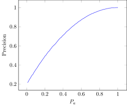
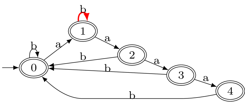
Let us show with an example how sensitive the model’s accuracy calculated by trace similarity is to the choice of random walk parameters. We take a concrete example based on the reference model Signature, adapted from the benchmark models provided in Krka et al. (2014). For readability, we used single symbols on transition labels and omitted transitions to error states. The reference model is shown in Figure 1(a), while Figure 1(b) shows the inferred model , obtained with MINT (Walkinshaw et al., 2016) — a state-of-the-art model inference tool — with its default configuration, on a set of 100 traces accepted by . To see the impact of different parameters of random walks on the precision of , we vary the termination probability (denoted with ) between and , while the choice of the outgoing transition is always done uniformly among the available alternatives. For each value of , 50,000 random traces are generated to assess the precision of . Figure 2 shows the result. When , the random walk always generates a trace of length zero (since the empty string is accepted by ), which is a true positive, and therefore the precision value converges to 1. On the contrary, as decreases, longer traces are generated and the precision value converges to 0.2. In this simple example, this range of values could have been predicted analytically because, for traces of length (), the number of true positives is (the set of true positives is the language determined by the regular expression ) while the number of false positives is (the set of false positives is the language determined by the regular expression ), and therefore . As a result, we can see that the precision value varies between 0.2 and 1.0 depending on the value of , implying that the result of trace similarity is extremely sensitive to the choice of the random walk parametrization. Unlike in this simple example, however, the effect of the random walk on the assessment result is in general difficult to predict analytically.
3.1.1. Statistical Estimation by Sampling
The sampling bias caused by the random trace generation is fundamentally unavoidable, because the sampled languages are in general infinite and there exists no uniform distribution over a discrete infinite set. There are, however, alternative methods to generate a random evaluation multiset (and then compute precision and recall using equation (1)) that allow for more control over the sampling bias.
The simplest method consists in generating traces by combining symbols randomly selected from the alphabet , without considering the models under analysis, thus making the sampling bias model-independent. This can be done, for example, by firstly selecting a random trace length , and then concatenating symbols, each one randomly selected from . The generated trace is then added to the evaluation multiset , and the process is repeated until a stopping condition is met (e.g., a certain number of traces has been generated). Note that, when the maximum length of a sample trace is fixed, it is possible to perform this trace generation in a way that ensures uniform probability distribution over : each trace length must be chosen with probability proportional to , and each symbol must be chosen with uniform distribution.
Despite its simplicity and its ability to reduce the sampling bias, compared to methods based on random walks like trace similarity, sampling from is rarely used in practice due to its computational cost: for most practical problems and large values of , the proportion of accepted by either or tends to decrease with , leading to most samples being true negatives, whose number does not contribute to the computation of either precision or recall. We will show instances of this problem experimentally in Section 6.
3.2. Model-Based Assessment
Walkinshaw et al. (Walkinshaw et al., 2008) proposed a new method based on methodologies from model-based testing (MBT), aimed at mitigating the sampling bias introduced by the random sampling and increasing the reproducibility of the results, as it is deterministic and thus not affected by the statistical uncertainty that comes from using a finite randomly generated evaluation set. The intuition is that MBT methods can deterministically generate a set of traces that is comprehensive (in the sense that any erroneous behavior of the inferred model would be detected) that can be used as evaluation set.
There are multiple MBT methods for DFAs (Chow, 1978; Bonifácio et al., 2008) that, given a reference model and an upper bound on the number of states the inferred model ( in our case) is allowed to contain, can check the equivalence of and by testing them on a finite set of traces, i.e., it can generate a set of traces such that, ideally, . The idea proposed by Walkinshaw et al. (Walkinshaw et al., 2008) is to compute precision and recall using the set of traces (generated using the MBT method of choice) as evaluation set .
As an example, let us describe how the W-method (Chow, 1978), a widely-used MBT method for DFA, generates a set of tests . Given the reference model and an upper bound to the number of states of denoted with , it constructs two sets of traces: a state cover (denoted with ) and a characterization set (denoted with ). The state cover is a prefix-closed subset of containing traces reaching each state of , i.e., . The characterization set is a subset of such that, for any pair of states with , it contains a distinguishing trace such that is an accepting state but is not, or vice versa. The test set generated by the W-method is then defined as , where and for two sets of traces and .
The comprehensiveness of ensures that any erroneous behavior in the inferred model will affect the accuracy metrics, and the way in which is generated does not favor specific parts of the model under analysis, leading to less skewed accuracy results when compared to statistical estimation. Nevertheless, using to measure the accuracy of an inferred model has three major shortcomings.
First, there are multiple approaches in the area of MBT for DFA with different aims. For example, the Wp-method (Fujiwara et al., 1991) is a further development of the W-method aimed at reducing the size of while providing the same guarantees. Since different approaches will generate different sets of tests , usually with different number of tests accepted or rejected by either of the models, they will also lead to different accuracy results.
Second, as already noted by Walkinshaw et al. (2008), MBT methods often generate a set containing a disproportionately large amount of traces not accepted by the reference model, which may lead to skewed accuracy results. Furthermore, can become exceedingly large if the difference between the number of states of and the number of states of is large. For example, in the W-method described above, the cardinality of grows with , where is the difference between the number of states. This is a significant issue especially in the context of model inference from positive examples only, where it is not unusual to obtain inferred models having a number of states that is one order of magnitude larger than the number of states of the reference model, making this type of assessment infeasible. This will also be shown experimentally in Section 6.
Third, although MBT guarantees that the generated will certainly contain a counterexample trace highlighting any incorrect behavior of the inferred model, each counterexample trace has the same “weight” on the computed accuracy metrics, even though it could represent a smaller or larger class of errors. Let us consider the example shown in Figure 3; it contains a reference model (Figure 3(a)) and two incorrect models (Figure 3(b)) and (figure 3(c)), which were manually created introducing the erroneous transitions highlighted in red. Both and have only false negative errors.


By enumerating all traces we verified that, for any trace length, has fewer false negatives than (e.g., for traces of length less than or equal to 10, has 11 false negative traces, while has 64 false negative traces). However, when the model accuracy is evaluated using the set of traces generated by the W-method, has 96% recall while has 98% recall (precision is 100% in both cases). This happens because individual false negative traces in do not represent an equal number of false negative traces in the inferred languages.
4. Measuring Accuracy with Trace Counting
To overcome the limitations of statistical and model-based accuracy evaluations, we propose to compute precision and recall, using analytical measures for the cardinality of the languages of true positives, false positives and false negatives — normally, restricted up to a finite maximum trace length to handle languages with unbounded traces.
In particular, the proposed cardinality measures should be: 1) deterministic, making the process repeatable and avoiding the convergence limitations of statistical methods; 2) comprehensive, accounting for every trace; 3) unbiased, giving each trace the same weight on the result; 4) model-independent, generating the same accuracy measurement on all models accepting the same language.
Notably, a statistical estimation in which all the traces (up to the prescribed maximum length) are sampled uniformly with the same probability (such as via the model-independent random sampling from discussed in Section 3.1.1) would converge to the same values we propose to compute analytically. This will be shown experimentally in Section 6.
4.1. Language Cardinality Measures
We propose to compute two classes of cardinality-based measures to evaluate the accuracy of an inferred model (the hypothesis ) against a reference model .
The first step is the construction of the languages corresponding to the definitions of true positive, false positive, and false negative, as required for the computation of precision and recall. These languages will be accepted, respectively, by the automata , , and defined as:
| (6) |
We can then use analytic combinatorics methods, as described in Section 2.3, to obtain the sequences , , of the number of traces of length accepted by , , and respectively — the cardinality of the languages accepted by the three automata intersected with the evaluation set .
Finally, we compose these elementary cardinality measures to compute the derived precision and recall metrics for assessing an inferred hypothesis model: cumulative-length and single-length.
Cumulative-Length. This type of assessment considers all the traces of length up to a provided value (i.e., the evaluation set is ). We compute the cardinalities
using the sequences of cardinalities of the languages accepted by the automata in Equation 6, and then compute precision and recall:
| (7) |
Our analysis does not mandate for a specific value of the maximum trace length . If any domain knowledge for the application under analysis is available and suggests the use of a particular value, this should be used. In the absence of this information, the user should consider that the choice of the maximum trace length may affect the assessment result — as we will investigate experimentally in Section 6.4.
Resolving to using very large values of so to approximate the asymptotic values of and (i.e., the limit of such measures for ) is appealing, but should be done with caution, since models with the same asymptotic values can exhibit different accuracy for shorter trace lengths. Nonetheless, the asymptotic values of precision and recall carry useful information. If the precision eventually converges to zero, the hypothesis language contains more false positives than true positives (in order of magnitude); if it converges to one, there are more true positives than false positives, while a value in between these extremes is achievable if the numbers of true and false positive have the same order of magnitude (including when they are both finite). Analogous considerations can be formulated for the asymptotic convergence of the recall measure in Equation (7) by comparing the orders of magnitude of the true positives and false negatives languages. We will further investigate experimentally the behavior of our cardinality-based accuracy metrics for large values of in Section 6.4444The analytical computation of such asymptotic values is usually non-trivial and will not be considered in this work. The interested reader may refer to “Part B: Complex Asymptotics” of (Flajolet and Sedgewick, 2009) for an extensive treatment of the subject..
Single-length Assessment. A second pair of cardinality-based assessment metrics can be obtained by computing precision and recall on the sublanguages of , , and restricted to traces of exactly length , i.e., the traces at the intersection of and the corresponding automaton.
Given a trace length, computing precision and recall is straightforward, using directly values from the sequences of cardinalities previously defined:
| (8) |
This assessment type can be used to build a more comprehensive picture of the model accuracy by repeating the assessment for every trace length within a range specified by the user. The result has multiple desirable features. First, is not sensitive to the parameter selection: the choice of the range of trace lengths over which the single-length assessment is repeated does not affect the result, but just defines the scope of the assessment. Second, it makes clear how the model accuracy changes across the trace lengths considered — a characteristic that current popular assessment methods do not highlight despite the fact that, in general, models do have variable accuracy depending on the trace length, as it will be observed in our experimental evaluation (Section 6). Third, it allows computing derived accuracy metrics that consider different trace lengths with different weight. This may be used, for example, to weight precision and recall on the frequency of trace lengths observed in a specific deployment of the system.
Although our method does not mandate for a specific range, it should be wide enough to cover all the possible behaviors of the models under analysis, for example ensuring that the upper bound of the range is at least equal to the number of states of the largest automaton under analysis.
5. Fast Computation of OGFs for Model Assessment
In our model assessment method we compute the values of precision and recall using the counts of true positives, false positives and false negatives, up to a finite maximum trace length. To obtain these counts without explicitly enumerating all the possible traces, we use analytic combinatorics (see Section 2.3), to count the number of different accepting paths on the automata accepting these languages.
To do so, the first step is to obtain the ordinary generating function (OGF) for the cardinality sequence of the language under analysis. This is generally done using the transfer matrix method (Flajolet and Sedgewick, 2009; Stanley, 2011), which relies on linear algebraic operations on the matrix representing the transition relation of the automaton (Flajolet and Sedgewick, 2009), resulting in its worst-case complexity being cubic in the state count. This section describes an alternative state elimination algorithm that, despite having the same worst case complexity, in practice in our preliminary evaluation performed significantly better than the transfer matrix method, by exploiting the sparsity of the transition matrix.
Our method is analogous to the state elimination algorithm by Brzozowski and McCluskey (Brzozowski and McCluskey, 1963) to generate a regular expression given a finite state automaton. While in the Brzozowski and McCluskey’s algorithm each transition is labeled with a regular expression indicating the language that causes traversing the transition, in our method it is labeled with the OGF of the cardinality sequence of that same language. The reduction rules used when a state is eliminated then allow us to progressively build the OGF through operations between rational functions.
Our method is presented in algorithm 1
and works as follows.
Given an input DFA, we construct (line 1) a directed graph , using digraphConstruction (algorithm 2):
each state of the DFA corresponds to one node of (distinct states correspond to distinct nodes), and the edge between any ordered pair of nodes of is labeled with the generating function of the sequence of cardinalities of the language of words of length one, containing the symbols causing the transition between the two corresponding states of the DFA. If the cardinality of this language is (i.e., there are symbols causing the transition from the source state to the destination state), the cardinality sequence is , thus the generating function on the corresponding edge of is . In addition, we add to a node called initial, an edge from initial to the node corresponding to the initial state of the DFA, a node called final, and an edge from each node corresponding to an accepting state of the DFA to final. All these additional edges are labeled with the generating function , which is the generating function of the cardinality sequence (i.e., of the language containing only the empty string). Adding these edges does not change the final generating function, but it is a simple way of dealing with multiple final states and transitions back to the initial state. Figure 4(a)


shows the example DFA taken from (Aydin et al., 2015) (which computes the OGF using the transfer matrix method), whereas Figure 4(b) depicts the graph constructed with these rules described above.
Then, at lines 1–1 of algorithm 1, we eliminate, one by one and using eliminateNode (Algorithm 3), all the nodes of except initial and final, as follows.
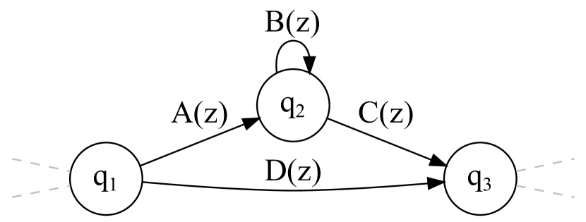
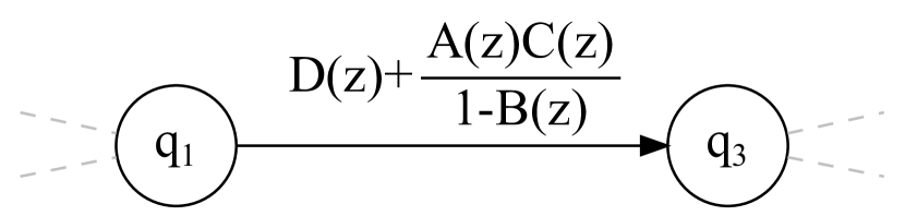
Let be the node to be eliminated; algorithm eliminateNode works by replacing every pair composed by one edge entering from a predecessor node and one edge exiting to a successor node , with a single edge from to , keeping into account the loop edge from to if present. The procedure computes the OGF on the new edges using the fact that union, concatenation, and Kleene star of regular languages translate to algebraic operations between the OGF of the cardinality sequences of the operand languages. Specifically: if and are regular languages, their concatenation is a regular language with ; if and are regular languages and (which in our case is a consequence of the automaton determinism), then their union is a regular language with ; if is a regular language with then (Kleene star) is a regular language with . As a result, Algorithm 3 computes the OGF of the Kleene star of the language that would be on the loop of the node to be eliminated (line 3), eliminates the loop (line 2) — otherwise the set of predecessors and successors subsequently defined would contain — and then iterates through the edges entering and exiting , updating the OGF on the edge from the predecessor node to the successor node as illustrated in Figure 5.
When initial and final are the only nodes left in , the OGF on the edge from initial to final is the OGF of the cardinality sequence of the language accepted by the DFA.
Figure 6 shows one possible sequence of state eliminations to obtain the generating functions of the DFA shown in Figure 4(a).


We remark the order with which the nodes are eliminated is not relevant for the correctness of the result. However, it does significantly affect the performance due to the cost of the operations between rational functions required to compute the generating functions on the edges involved in each elimination. A simple heuristic that proved to be beneficial in our experiments is choosing first the node with the lowest OGF degree555The OGF degree is defined as the maximum of the degrees of its constituent numerator and denominator polynomials. on the self loop (thus the nodes with no self loop are eliminated first).
6. Experimental Evaluation
In this section, we report on the experimental evaluation of our model assessment method in terms of the following aspects. First, since the cumulative-length assessment requires, as an input parameter, a maximum trace length, we investigate the impact of changing its value on the model assessment results. We also analyze whether the asymptotic values (i.e., the results obtained when the maximum trace length go to infinity) are useful to characterize the model accuracy. Second, to better understand to what extent the model assessment results differ depending on the methods used, we compare the results obtained using our method with the results obtained using existing methods, specifically the statistical estimation and MBT-based methods. Third, in Section 4, we claimed that a statistical estimation in which traces having the same length have the same probability of being sampled would converge to the same results obtained by our single-length assessment method. We will verify this experimentally by comparing the single-length assessment and a model-independent sampling of in terms of the precision and recall values. Finally, we evaluate the applicability of our method on models inferred using well known model inference approaches.
To summarize, we address the following research questions:
-
RQ1:
How does the choice of the maximum trace length affect the model assessment results?
-
RQ2:
How do the values of precision and recall obtained using our method compare with the results obtained using other evaluation methods?
-
RQ3:
Is the single-length assessment over a range of lengths a usable alternative to the statistical evaluation of model accuracy using model-independent sampling of ?
-
RQ4:
Is our method applicable to the assessment of inferred models representing aspects of actual software systems?
6.1. Evaluation Subjects
To evaluate model assessment methods, we need various pairs of reference and inferred models. We describe how we select reference models and generate inferred models from them below.
Reference Models
We selected 41 publicly available reference models, taken from existing studies (Pradel et al., 2010; Krka et al., 2014); all of them have a well-documented origin and were previously used in the model inference literature.
Pradel et al. (2010) selected 32 commonly used classes from the Java SDK API and identified their method ordering constraints using the API documentation and well-known reference books. These constraints were then translated into reference models representing all possible valid traces of method calls. The resulting reference models are publicly available on the authors’ website666http://mp.binaervarianz.de/icsm2010/index.html. These models were used also in previous work on model inference (Busany et al., 2019).
Krka et al. (2014) selected 9 open-source libraries, found the corresponding reference models (manually specified in previous work), and checked them manually for inconsistencies. These models were checked against execution traces collected from actual executions of software using those libraries, and the transitions on methods that were never invoked in the collected traces were eliminated. The resulting reference models are publicly available on the authors’ website777https://softarch.usc.edu/wiki/doku.php?id=inference:start. These models have been used also in previous work (Walkinshaw et al., 2016; Le et al., 2015)
Inferred Models
Ideally, the inferred models should be generated using model inference engines on traces produced by executions of actual software systems. Unfortunately, we were not able to find and execute the exact versions of the software systems represented by the 41 reference models, to collect their execution traces. As an alternative, we used the same type of random walk described in Section 3.1 to generate a set of random traces for each reference model, and then we processed each set of traces using different model inference engines. As for the random walk parameters, we used the termination probability and the uniform probability for selecting an outgoing transition among available transitions following Walkinshaw et al. (2013). For each reference model, we repeated the random walk until at least 100 traces were generated and each state of the model had been visited at least four times, as suggested by Busany et al. (2019). From each set of traces we inferred two models, using two different model inference algorithms: -tails (Biermann and Feldman, 1972) (the most well-known model inference algorithm) and MINT (Walkinshaw et al., 2016) (a state-of-the-art model inference technique). Before the accuracy assessment, the inferred models were minimized, through standard (language preserving) automata minimization.
It is worth noting that, in the area of model inference, it is common practice to use randomly generated traces when traces coming from actual software executions are not available (e.g., (Busany et al., 2019; Lo et al., 2012; Walkinshaw and Bogdanov, 2013; Walkinshaw et al., 2013)). Moreover, model assessment is independent of how inferred models are generated, thus is not a major issue in our evaluation. Nevertheless, we will discuss this as a potential threat to validity in Section 6.8.
To summarize, our experimental evaluation is based on 82 test subjects (pairs of reference and inferred models): 41 reference models, with two inferred models each. Table 1 shows the size of the reference and inferred models in terms of the minimum, the average, and the maximum number of states and transitions.
| State count | Transition count | ||||||
| Min | Avg | Max | Min | Avg | Max | ||
| Reference | 2 | 9.2 | 41 | 7 | 77.8 | 465 | |
| Inferred | 2 | 349 | 2060 | 5 | 752 | 4994 | |
6.2. Evaluation Settings
We performed the assessment of all the 82 test subjects using our implementation of trace similarity, MBT-based assessment, and our method with trace counting, all developed in Java and publicly available (see Section 6.3).
All the experiments were executed on an AMD EPYC 7401P (24 cores, 48 threads) with 448 GB of RAM. Since the implementation of our evaluation method is single-thread, 24 evaluations were executed concurrently.
The evaluation runtime of every model assessment performed in our evaluation was subject to a timeout of two days. It is worth pointing out that all the single-length and cumulative-length assessments on the same test subject require the same evaluation runtime. The reason is that this evaluation runtime is dominated by the time required to compute the generating functions, which are the same for all assessments of the same test subject.
6.3. Data availability
To support open science and enhance the reproducibility of our evaluation, we provide a replication package888https://doi.org/10.6084/m9.figshare.24932799 including all the artifacts: the source code, the reference models and the inferred models used.
6.4. RQ1: Input Parameter Sensitivity
Methodology
As described in Section 4, our method can be applied in two ways: cumulative-length and single-length assessments. The single-length assessment repeated over a range of trace lengths is not sensitive to parameter changes: the range changes just the scope of the assessment, i.e., for which lengths the values of precision and recall are computed, without affecting the output values themselves. To evaluate the parameter sensitivity of the cumulative-length assessment, we computed the precision and recall values varying the only parameter (i.e., the maximum trace length) from 0 to 200 in steps of 1.
Results
All the assessments of 61 of the 82 test subjects terminated within the 2-day timeout. Figure 7 shows how the precision and recall values vary depending on the maximum trace length parameter; each line is a result for one test subject.
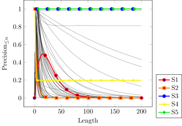
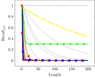
The foremost takeaway of the evaluation results is that the choice of the maximum trace length parameter does indeed affect the computed accuracy values, and it does so differently, depending on the inferred model. The results highlighted the prevalence of cases in which precision and/or recall values cover a large part of the range , depending on the parameter value. Specifically, among the 61 test subjects that finished within the timeout, 20 have a precision value (and 54 have a recall value) that covers the entire range , depending on the maximum trace length parameter. This emphasizes how — for any choice of a single value of the maximum trace length — some relevant information about the model accuracy is inevitably lost, leading to possibly misleading results.
Figure 7 also shows the variety of trends that the precision and recall values can have, as the maximum trace length is increased: e.g., convergence to 0 with and without a peak, constant equal to 1, and convergence to . In the figure we have highlighted (with colors and special markers) five test subjects that, together, cover the most common trends we observed in the results of this experiment. Appendix A gives further details on how we selected these test subjects, and Appendix B describes the selected test subjects in more detail. Table 2 summarizes the characteristics of these representative test subjects.
| Reference model | Inference approach | Inferred model | ||||
| Name | States | Trans. | States | Trans. | ||
| Subject 1 (S1) | java.net.URL (Pradel et al., 2010) | 5 | 57 | MINT | 718 | 993 |
| Subject 2 (S2) | SMTPProtocol (Krka et al., 2014) | 3 | 14 | MINT | 24 | 110 |
| Subject 3 (S3) | StringTokenizer (Pradel et al., 2010) | 4 | 14 | 2-tails | 83 | 175 |
| Subject 4 (S4) | Signature (Krka et al., 2014) | 3 | 7 | MINT | 15 | 63 |
| Subject 5 (S5) | StringTokenizer (Krka et al., 2014) | 4 | 7 | 2-tails | 30 | 61 |
Furthermore, Figure 7 shows that the asymptotic value999 We determined the asymptotic value by manually checking to which value the accuracy stabilizes. There were some cases (seven for the precision value, four for recall value) in which we were not able to determine the asymptotic value because, within the observed range, it was not clear around which value it stabilized. can be reached through different paths, with fast or slow convergence, and with or without local minima or maxima. This confirms that judging or comparing model accuracies according to the asymptotic value of precision and recall can be misleading, since models with the same asymptotic accuracy generally can have different accuracies for shorter traces.
Although investigating the asymptotic accuracy of models obtained with current inference methods is outside the scope of this paper, an interesting observation is that the asymptotic values of the accuracy metrics are generally either zero or one. This is because the precision and recall values are quotients between language cardinalities that tend to infinity as the maximum trace length considered is increased, therefore the quotient often goes to zero or one depending on the relative growth rate of the languages in Equation 1. In our evaluation, the most common asymptotic value is zero: 45 subjects have a precision value converging to zero, while 55 have a recall value converging to zero. The number of subjects having accuracy converging to a value greater than zero and smaller than one is only three for precision and two for recall. This is an observation that is outside the scope of this paper, and may not generalize to models obtained with different inference methods; it will be further investigated in future work.
It is difficult to relate accuracy trend patterns (observed a posteriori) with characteristics of the inferred model such as the topology. However, it is worth noting that inferred models accepting finite languages (identified by the absence of loops) generally indicate that the inference algorithm was not able to generalize the training data, resulting in inferred models with good precision but poor recall. Some patterns that we observed a posteriori are discussed in Appendix B. It is also worth noting that the analysis of the generating function associated to the models’ cardinalities can predict the asymptotic trends (Flajolet and Sedgewick, 2009); nevertheless, this type of analysis is beyond the scope of this paper.
Answer to RQ1
The maximum trace length parameter does affect the computed cumulative-length precision and recall values, and it does so differently, depending on the inferred model. This parameter should be tuned, case by case, to a value that is relevant for the application under analysis. If no domain knowledge is available, it is preferable to consider how precision and recall values change considering different trace lengths, using the single-length metrics.
6.5. RQ2: Comparison of Model Assessment Methods
This section discusses how the results generated by the assessment methods described and discussed in the paper compare with each other. In particular, we will examine trace similarity, MBT-based assessment, cumulative-length assessment, and single-length assessment.
Note that the model assessment methods discussed in this paper can be classified into two types depending on their output types: trace similarity, MBT-based assessment, and the cumulative-length assessment are all methods that return one pair of precision and recall values, while the single-length assessment instead returns one pair of precision and recall values per trace length in the given range (which is a parameter of the method). These two types cannot be directly compared. For this reason the comparison proposed in this section is divided in two parts.
In the first part, we will compare trace similarity, MBT-based, and cumulative-length, with the goal of understanding the consistency and the differences between the computed precision and recall values across the different assessment methods and different parameter values.
In the second part, we will discuss the single-length assessment results in relation with the results generated with the other currently used methods. In this case a direct comparison is neither possible nor meaningful, due to the different output type. To make them comparable, we will condition the other assessment methods on the trace length: the evaluation sets generated by these methods will be partitioned according to the trace length, and the subsets will be used to compute one pair of precision and recall values per trace length, which can then be directly compared with the results from the single-length assessment.
Comparison of Trace Similarity, MBT-based, and Cumulative-Length Assessments
As discussed above, we first compare trace similarity, MBT-based, and cumulative-length.
Methodology
To understand the consistency and the differences between the computed precision and recall values across the different assessment methods, we run the methods on the 82 test subjects, with the following parameters settings.
Trace similarity requires defining how to make the nondeterministic choices needed to conduct the random walk (i.e., whether to terminate the walk, and which available transition should be traversed — see Section 3.1). This has a direct effect on the sampling bias, thus affecting the assessment results. In our setup, the selection of the outgoing transition to be traversed was done uniformly among the available alternatives, as it is often done in practice (e.g., (Walkinshaw et al., 2013; Lo and Khoo, 2006a)). Regarding the termination of the trace when a final state is reached, we found different approaches in the model inference literature. Sometimes the termination probability is a function of the outdegree of the accepting state (e.g., as in reference (Walkinshaw et al., 2013)), sometimes is not (e.g., as in reference (Lo et al., 2012)). To highlight how this choice may affect the assessment result, we used a fixed termination probability , and we executed the trace similarity assessment setting to three values (0.02, 0.1 and 0.5), thus obtaining three pairs of precision and recall values for each test subject. Trace similarity also requires specifying the target size for the evaluation set , which in our experiments was set to 100,000 traces. To further ensure adequate model coverage, we continued adding traces to beyond the target size, until each transition of the model was followed at least 10 times (as proposed in reference (Lo and Khoo, 2006a)), or a 30-minute time limit was reached. As a result, in some cases we generated more than 100,000 traces.
The MBT-based assessment requires a model-based testing method for finite state automata, to generate the evaluation set . We use the W-method, as done by the original proponents of the method.
The cumulative-length assessment requires a parameter indicating the maximum length of the traces to be considered. Since there is no “correct” value to choose in the absence of domain knowledge for a specific test subject, we evaluate the results when varying the parameter from 0 to 200 in steps of 1.
Results
All the model assessments performed using trace similarity returned a result within the timeout. The cumulative-length assessments terminated within the timeout for 61 of the 82 test subjects (for all parameter values), while for the remaining 21 subjects a timeout occurred during the computation of the generating function. The MBT-based assessment terminated within the timeout only in two of the 82 cases under analysis. The reason is that the cardinality of the evaluation set generated with the W-method grows with , where is the difference in the number of states between the inferred and reference model, therefore the method is usable only when the reference and inferred models have a similar number of states. This is rarely the case in our set of test subjects: the difference is on average 247 (). Due to the lack of a sufficient number of results from the MBT-based assessment, we omit this method in the rest of the comparison.
Before we compare the trace similarity and cumulative-length assessment results, it is worth focusing on how trace similarity is affected by the termination probability of the random walk. Table 3 shows the effect of on the average length of the traces generated in our experimental evaluation. These are consistent with an exponential distribution, however we remind that the relationship between termination probability and distribution of trace lengths is model dependent, and our experiments lead to this distribution only because most of the non-error states of the models under analysis are accepting states.
| Mean trace length | |
| 0.5 | 1.99 |
| 0.1 | 11.28 |
| 0.02 | 49.45 |
Table 4 summarizes the absolute difference between the model accuracy evaluated using trace similarity with different random walk termination probability . For example the mean absolute difference between the precision value computed using trace similarity with a random walk with , and the precision value computed using trace similarity with a random walk with , is (), with indicating percentage points. This difference indicates that the choice of the random walk parameters values can affect the trace similarity result in a way that does not allow us to reliably determine the model accuracy. Note that a larger difference in the parameter leads to a larger difference in the measured accuracy (e.g., line 1 vs line 3 of Table 4). This is explained intuitively in terms of the sampling bias discussed in Section 3.1: a random walk with higher termination probability will generally produce shorter traces, and we know, from the RQ1 results in Section 6.4, that in most cases the model accuracy is higher on shorter traces.
| Mean | ||
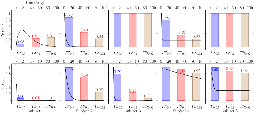
Figure 8 shows the comparison of the precision and recall values computed using trace similarity and our cumulative-length assessment, for the five representative test subjects selected in RQ1. To improve the readability, the range of the trace length parameter for the cumulative-length assessment shown in the figure is from 0 to 100. The same information is available for all test subjects in the supporting material (see Section 6.3). Note the three different trace similarity assessments per test subject (using different values of the parameter of the random walk).
The most important observation is that both trace similarity and cumulative-length results values are different in most cases, and vary over a large range of values depending on the methods’ parameters.
A closer look reveals a consistency between the trend of the accuracy results computed using trace similarity as is decreased, and the trend of the accuracy results computed by the cumulative-length assessment for longer traces: in all subjects for which the cumulative-length assessment shows decreasing model accuracy for longer traces, also the trace similarity assessment shows decreasing accuracy as is decreased from 0.5 to 0.02. Analogously, the cumulative-length assessment for subject S1 shows an (initially) increasing precision, and the corresponding trace similarity result is also consistent with this trend. The reason behind this consistency is the effect of the random walk termination probability on the length of the traces generated by the random walk, as discussed before. However, it is important to stress that the distribution of trace lengths generated by the random walk is not enough to fully capture how the sampling bias affects the trace similarity result, because also different traces of the same length may have different probabilities of being generated. The nondeterministic choices required to conduct the random walk can be performed in a variety of ways, and their effect on the result is model-dependent. On the other hand, the cumulative-length assessment has only the maximum trace length parameter, whose effect can be intuitively understood, making it easier to tune. Section 6.5 will include a scenario in which trace similarity and cumulative-length assessment diverge due to this effect.
Furthermore, in Figure 8 we can observe that for some test subjects all the model assessment methods compute the same value (100%) for precision. We manually verified that in these cases the inferred language is a subset of the reference language, hence the evaluation set cannot contain false positive traces, regardless how it is generated, and thus the computed precision value is always 100%.
Comparison of Statistical Estimation and Single-Length Assessment
We now turn our attention to the results of the single-length assessment over a range of trace lengths, and how it compares with the results of trace similarity.
Methodology
As discussed above, a direct comparison is not possible, since the single-length assessment returns one pair of precision and recall values per trace length, while trace similarity returns one pair of precision and recall values overall.
To obtain comparable results, we will condition the trace similarity on the trace length, by partitioning each evaluation set according to the trace length. This will allow us to use the resulting subsets to compute one pair of precision and recall values per trace length, and it will also allow us to look at the distribution of the traces in across different trace lengths. In fact, we will initially focus on this distribution, which is the first effect of the sampling bias induced by the random walk mentioned in Section 3.1. Then, we will compare the values of precision and recall for different trace lengths (from 1 to 100 in steps of 1). Since our single-length assessment has no sampling bias, any difference in precision or recall value for a specific trace length implies statistical noise and/or the non-uniformity of the sampling induced by the random walk (i.e., the second effect of the sampling bias as mentioned in Section 3.1).
Results
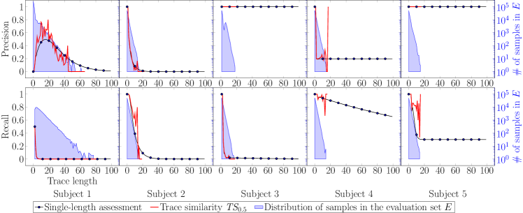
The results for the five representative test subjects previously used in RQ1 are shown in Figure 9.
In each plot, the red line and the black line with markers represent how the accuracy metric values (left y-axis) computed by trace similarity conditioned on the trace length and the single-length assessment, respectively, vary depending on the trace length (x-axis). In addition, the solid area filled in blue indicates the number of samples (right y-axis) in the evaluation set for each trace length (x-axis). Note that, in some of the plots, the red line and the blue area do not exist after a certain trace length, meaning that the random walk generated an empty and no precision and recall values were computed by trace similarity.
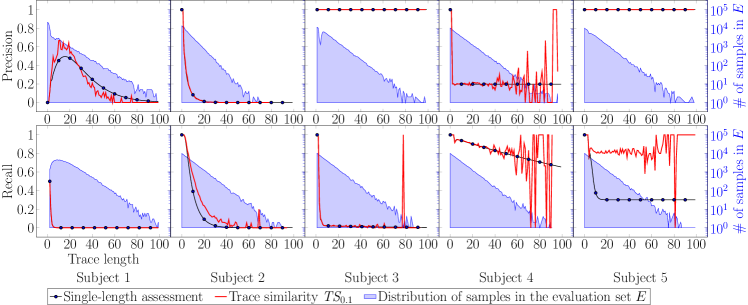
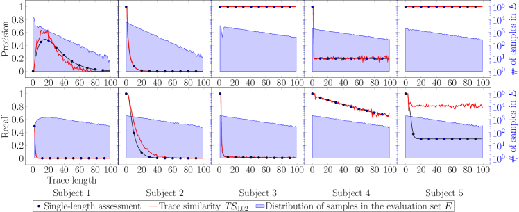
Based on the results shown in Figure 9, we can make the following observations.
-
•
The distribution of samples highlights how shorter traces are more likely to be sampled, and how the distribution of samples depends both on the random walk parameters and on the model upon which the random walk is performed. For example with (Figure 9(a)) the distribution of samples for subject S1 contains longer traces, compared to the other test subjects. Conversely, with (Figure 9(c)) the distribution of samples for the precision assessment of subject S1 contains shorter traces, compared to the other test subjects.
-
•
The random walk can introduce a sampling bias between traces having the same length. This is particularly visible in Figure 9(c), in the recall plots of subject S5, which show a difference between trace similarity conditioned on the length (red line, which converges to 0.8) and the single-length evaluation (black line, which converges to 0.3). This observation explains why in Figure 8, in the case of subject S5, the recall values obtained using standard trace similarity consistently exceed the recall values obtained using our cumulative-length assessment, despite the fact that the inferred model consistently shows a 0.3 recall value for traces having a length greater than 20. Note that in the other test subjects, the plots of trace similarity conditioned on the trace length, and those of the single-length assessment show the same trend, highlighting how this effect is model-dependent.
One might think that using an assessment method like trace similarity adjusted to assess the accuracy for long traces could be used to evaluate the asymptotic behaviour of the model accuracy; however, this approach could give misleading results. If the asymptotic behavior of the model accuracy converges to a value that is neither zero nor one, we have observed (in Subject S5) that trace similarity may converge to a wrong value. If the asymptotic behavior converges to zero or one (the most common case), it is yet to be proved that the trace similarity bias would not affect this behaviour. Moreover, although most models have precision or recall converging to 0 or 1, the speed at which they do so is relevant for practical purposes (a model accuracy could be asymptotically zero, but still acceptable for short traces), and this information would be lost using this approach.
Answer to RQ2
The sampling bias affects the trace similarity result in a way that is hard to predict a priori, because it depends on both the topology of the model and the parameters of the random walk. When trace similarity is compared to the cumulative-length assessment, the conclusion is that the choice of the parameter values of both assessment methods affect the result to an extent that does not allow us to reliably determine the model accuracy, thus preventing a meaningful comparison among different models in terms of accuracy, or among the accuracy values of the same model measured with different methods.
On the other hand, the single-length assessment is not affected by sampling bias because it measures the model accuracy for each trace length in the given range, considering (for each length) all the possible traces. Leveraging this characteristic, we compared the single-length assessment with trace similarity conditioned on trace length and analyzed the effect of non-uniform sampling among traces of the same length. We found that trace similarity can indeed converge to different and possibly misleading accuracy values due to this model-dependent bias. We also examined the distribution of trace length generated by the various random walk in trace similarity, noticing how shorter traces are more likely to be sampled, and how this effect depends on the model topology and the parameters of the random walk.
6.6. RQ3: Single-length assessment and model-independent sampling of
The goal of RQ3 is to compare, in terms of precision and recall, the single-length assessment we proposed and a model-independent sampling of inspired by the observation made in Sections 3.1.1 and 4. It is possible to statistically assess precision and recall using a sampling method that generates traces by combining symbols randomly chosen from the alphabet, rather than through random walks on models. In practice, however, using this method is feasible only for short trace lengths, because to evaluate precision (respectively, recall) it is necessary to generate traces that are accepted by the inferred (respectively, reference) model. This generation process becomes infeasible with real-world models and long traces, due to the gap between the exponential growth of and the slower growth of the size of the accepted language of length , as the length is increased. Nonetheless, this approach has the advantage of controlling the sampling bias (which becomes model independent), enabling sampling with uniform distribution over a finite subset of .
Answering this research question will let us check experimentally whether a statistical estimation of the model accuracy (in which all the traces having the same length have the same probability of being sampled) generates the same results as our single-length assessment. If the results show consensus between the two assessment methods, they will confirm that our method is a usable alternative to the statistical evaluation of model accuracy using model-independent sampling of .
Methodology
For each test subject, we computed precision and recall for each trace length starting at 0 and increasing it until a one-hour timeout was reached. This was done using Algorithm 4, which takes as input the reference model , the inferred model , the accuracy metric to be computed (precision or recall) and the trace length for which to compute it. The algorithm generates traces without considering the reference or the inferred model, by concatenating symbols randomly selected from the alphabet with uniform distribution. Each generated trace is then tested against the models: if is precision (respectively, recall), the trace is tested against (respectively, ), to determine whether it is part of the inferred (respectively, reference) language. If this is the case, the trace is further tested against (respectively, ) to determine whether it is a true positive. This is repeated until 1000 “useful” traces are generated, i.e., traces that are accepted by (respectively ) and therefore contribute to computing the metric. The target number of useful traces is a compromise between the scalability and the noise of the evaluation. It was chosen empirically, and deemed appropriate because it gives a 99% chance that the real precision/recall value is within ±4.08% of the measured value. Note that the maximum trace length reached with this model assessment method is model-dependent, since it depends on the proportion of traces in accepted by the models under analysis. In fact, it may differ even between precision and recall on the same test subject, since the proportion may be different between reference and inferred model.
Finally, we compared the resulting precision and recall values with the single-length assessment results.
Results
The differences between the model accuracies obtained using the single-length assessment and the model-independent sampling of (computed using all the trace lengths for which both results are available) are summarized in Table 5.
| Mean | ||
The small differences between the methods’ results are caused by the sampling error intrinsic in any accuracy measure performed using randomly generated samples, and are within the margin of error expected for the used number of samples. This confirms that a statistical estimation in which all the traces of the same length have the same probability of being sampled generates the same results as our single-length assessment, in line with your discussion in Section 4.
To have a closer look at the results for individual test subjects, Figure 10
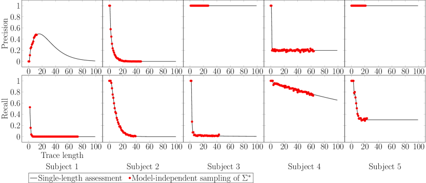
shows the results of the same five representative test subjects previously used in RQ1 and RQ2. The results obtained using the model-independent sampling of are represented by red markers (note the different ranges of trace lengths for which the results are available, due to the timeout), while the single-length assessment is represented by the black line. We remark the two methods exhibit a similar trend also on test subject 5, for which instead the trace similarity method returned different results due to the non-uniform probability distribution of traces having the same length, induced by the random walk.
Answer to RQ3
The precision and recall values obtained using the single-length assessment we proposed are consistent with those obtained using a model-independent sampling of . This implies that our method is preferable, because it is not limited to short trace lengths, and because, being deterministic, is not affected by statistical noise.
6.7. RQ4: Practical applicability on inferred models
This section discusses the practical applicability of our approach by evaluating its scalability with respect to the complexity of the models under analysis, measuring the execution time of each assessment on each test subject.
Methodology
Model complexity is widely studied, and can be measured in a variety of ways, with different complexity metrics appropriate in different scenarios. We will evaluate the scalability of our method with respect to two different model complexity metrics: deterministic state complexity (Yu, 2001) and star height (Eggan, 1963). Specifically, given a regular language , these metrics are defined as follows. The deterministic state complexity is defined as the number of states of the minimal DFA accepting . We will refer to this measure simply as the “number of states”, since all the automata used in this work are in their minimal form. The number of states is a commonly used model complexity metric in the field of model inference (Walkinshaw et al., 2016; Lo and Khoo, 2006b). The star height of is the minimum star height among all the regular expressions representing , where the star height of a regular expression is the maximum nesting depth of Kleene star operators in the expression. Though the start height is less common, it is a better predictor of the execution time of our assessment method since this is dominated by the computation of the OGFs. Referring to the OGF computation algorithm described in Section 5, it can be seen that an automaton without closed cycles leads to intermediate OGFs that are easy to compute since they are polynomials (instead of rational functions) generated using only sums and products of polynomials. Conversely, all cycles present in the automaton under analysis must eventually be eliminated during the OGF computation by composing the intermediate OGFs using sums, products, and quotients of rational functions. Intuitively, languages with higher star heights are likely to have more closed cycles in the corresponding DFA representation, increasing the complexity of the OGF computation, whereas a star height of zero indicates a finite language (thus with a corresponding DFA with no loops) of which the OGF is a polynomial of finite degree that is easy to compute.
We should note that the star height is by no means a complete metric; the cost of each state elimination operation in the OGF computation of Section 5 is hard to predict a priori, because it depends on the complexity of the rational functions involved. Nonetheless, developing a new ad-hoc structural complexity metric for the OGF computation is outside the scope of this work.
Finding the minimum star height of a language is a notoriously hard problem (Kirsten, 2005). Therefore, in our evaluation, we use an approximated value obtained by transforming the inferred model in a regular expression using the Brzozowski and McCluskey algorithm (Brzozowski and McCluskey, 1963) and then counting the maximum nesting depth of Kleene star operators in this expression.
Note that both reference and inferred models influence the execution time. However, in our experiments the size of the inferred model is one or two orders of magnitude larger than the size of the reference model: therefore we consider the effect of the latter negligible.
Since the differences in execution times between different assessments (single-length and cumulative-length) of the same subject are negligible, we give one execution time per test subject rather than per assessment. This is because the execution time is dominated by the computation of the OGFs, which is the same for all the assessments on the same test subject.
Results
Figure 11(a) shows the number of subject assessments completed over time. On one hand, 21 test subjects assessments did not finish within the timeout, and when the timeout occurred all of them were in the OGF computation phase. This confirms that the execution time of our method is dominated by the computation of the OGFs. Among the subject assessments that did not finish within the timeout, the minimum state count was 68 and the maximum was 2061, while the minimum approximated star height was 13 and the maximum was 304. Even though our method takes longer than the trace similarity method (which finished all executions within the timeout, with an average of only 168 seconds), recall that the results obtained through the trace similarity method are biased, as discussed in the previous research questions. On the other hand, 41 of 82 subjects had an assessment execution time of less than one minute, showing the practical suitability of the method. Additionally, a benefit of our method is that the OGFs, once generated, can be reused to perform further analyses with different parameters with negligible overhead.
Note that, although the OGF computation is time-consuming in our method, it is significantly more practical than a naive method that enumerates all the possible traces up to a certain length. Let us consider a reference model with an alphabet size of 21, which is the average alphabet size of the reference models used in our experiments. With this alphabet size, assessing the accuracy for traces up to a modest length of 15 would require evaluating traces against the reference and inferred models. Even under the overly optimistic assumption that a modern CPU at 4 GHz could test one execution trace against one model in one clock cycle, this assessment would require more than 1000 years.
Figure 11(b) shows the correlation between number of states of the inferred model, and execution time. The largest model successfully assessed had 1465 states, and was assessed in . The Pearson correlation coefficient between execution time and number of states was 0.07, highlighting how inadequate is this complexity metric to capture the computational complexity of the assessment.
Figure 11(c) shows the correlation between star height and execution time. The most complex inferred model successfully assessed had an approximated star height of 38 (i.e., the maximum nesting depth of the Kleene star operator in a regular expression accepting the inferred language was 38), and was assessed in — the longest execution time encountered among the test subjects that finished within the timeout. The Pearson correlation coefficient between star height and execution time was 0.51, implying that the start height can be a rough indicator of the execution time of our method.
Although the experiments were executed on a multicore system, our current implementation is still sequential, thus the performance metrics in this section are to be considered for a single core.
Answer to RQ4
Despite the inadequacy of widely adopted model complexity metrics, we report that our approach was able to assess inferred models representing aspects of actual software systems, using commodity hardware and despite being at a prototype stage.
6.8. Threats to validity
There are a number of factors that could impact the validity of our experimental results.
Choice of metrics. The choice of the accuracy metrics used in this evaluation could threaten the validity of our results if the metrics fail to capture adequately the model accuracy. To mitigate this threat we used precision and recall (Tharwat, 2020), which are well known metrics and have often been used in the area of model inference (Lo and Khoo, 2006a; Pradel et al., 2010; Walkinshaw et al., 2016; Krka et al., 2014; Polyvyanyy et al., 2020; Walkinshaw et al., 2008). Moreover, this risk is also partially mitigated by the fact that the proposed assessment method can be adapted to compute additional metrics (e.g., specificity or F-measure) without affecting the scalability.
The choice of the metric used to capture the model complexity in the evaluation of our method scalability could also pose a construct validity threat. To minimize this risk, we provided results using two different complexity metrics: model state count and language star height.
Reference models used. Using certain reference models could limit the generalizability of our results. To mitigate this issue, we considered a variety of reference models (41 in total), obtained from two different publicly available sources we found in the model inference literature (Pradel et al., 2010; Krka et al., 2014).
Training set generation and model inference setup. Due to the lack of a suitable and widely accepted model inference benchmark suite containing traces of real software executions, we used random walks on the reference models to generate the traces fed to a model inference method. This could introduce a bias in the training set, which may become a bias in the corresponding inferred models. Similarly, also the choice of the inference method (and its parameter values) could introduce a bias in the inferred model. Nevertheless, the model assessment method proposed in this paper and considered in our evaluation is independent of the method used for generating inferred models. Furthermore, we used the same evaluation subjects (i.e., pairs of reference and inferred models) for the model assessment methods used in our comparative evaluation, yielding fair comparison results. Moreover, testing inference methods using traces generated from random walks is common practice (Busany et al., 2019; Lo et al., 2012; Walkinshaw and Bogdanov, 2013; Walkinshaw et al., 2013).
Input parameters of other assessment methods. The comparison discussed in RQ2 is affected by the parameters of the considered assessment methods, e.g., the characteristics of the random walk used for trace similarity. To obtain results that are representative of how the assessment methods are is used in practice, our choice of parameter values was guided by what is frequently used in the literature. Nonetheless, different method parameters would in general lead to different results.
Statistical noise. Although single-length, cumulative-length, and MBT-based assessment methods are deterministic, trace similarity involves randomness, which could affect the evaluation results. However, due to the low computational cost for generating traces through random walks and checking them against a model, we were able to perform the trace similarity assessment using at least samples, ensuring low statistical noise.
Errors in the implementation. We used a prototype implementation of our method, which may contain faults. Moreover, in order to develop a self-contained solution that does not rely on external algebra systems such as Wolfram Mathematica (Inc., 2022) or Maple (Waterloo Maple, Inc.., 2022), the algebraic system used to perform operations on rational functions was implemented by us from scratch: it may also contain faults. To mitigate the issue, we performed systematic sanity checks by comparing the language cardinalities obtained using different counting methods.
7. Related Work
Our method is related to the work done in the area of model assessment and trace (model) counting101010This area of research is generally called model counting. In our context, this name could be confusing, since we have already used the term model to indicate a representation of an aspect of a system. To avoid any confusion, hereafter we refer to it as trace (model) counting..
7.1. Model Assessment
As discussed in Section 3.1, Lo and Khoo (2006a) proposed a method called trace similarity for empirically assessing the accuracy of inferred models against reference models, both in the form of probabilistic or non-probabilistic finite-state automata. The method measures the accuracy in terms of precision and recall using traces randomly generated from the models. Specifically, for a reference model and an inferred model , they defined recall as the percentage of traces generated by that are accepted by and precision as the percentage of traces generated by that are accepted by . They also proposed an algorithm called TraceGen that generates a set of random traces from a model with the aim of covering every transition in the model at least times, where is a coverage parameter. Lo et al. (2012) later extended the trace similarity method to additionally assess the accuracy of inferred models in terms of specificity, which is a metric indicating the ability to correctly reject illegal behaviors. One common issue of these methods, as discussed in Section 3.1, is that the accuracy of inferred models depends on the traces drawn according to a certain probability distribution imposed by the random trace generation. Our method resolves this issue by computing precision and recall values that consider all the traces, up to a user-defined arbitrarily large maximum length.
As discussed in Section 3.2, the aforementioned issue was also acknowledged by Walkinshaw et al. (2008), which addressed it by adapting the W-Method (Chow, 1978) (originally developed for model-based software testing to generate a set of traces covering all distinguishable runs of the model under test) to generate a “representative” trace set that covers all the model behaviors without privileging any specific one. Although this solution guarantees to cover all behaviors, it could still return misleading results (e.g., an inferred model having fewer counterexamples could obtain a lower accuracy value) since it does not consider the number of accepted traces affected by each behavior, which is something that our method does — up to a finite maximum trace length set by the user. Furthermore, as shown in our evaluation results, the MBT-based method is not scalable due to the exponential growth of the cardinality of the representative set with the number of different states between reference and inferred models.
Recently, Polyvyanyy et al. (2020) have proposed a framework that compares reference and inferred models in terms of their languages (i.e., the languages accepted by the models). While they defined precision and recall similarly to ours (i.e., Equation 7), they overlooked the usage of language cardinality, arguing that it is useful only for finite languages. Instead, they suggested framework instantiations using topological entropy as a language measure which, intuitively, measures the increase in the variability of the words of the language as their length goes to infinity. It is not clear whether, using this measure, an inferred model with fewer counterexamples would always obtain a higher accuracy value, even when the counterexample languages of the two inferred models are not in a subset-of relationship. In our method, all the traces up to the maximum trace length specified by the user are considered, and they all have the same weight on the result. Moreover, the maximum trace length parameter can be set either to a value that is relevant for the application under analysis, or to a very large value, resulting in effectively computing the asymptotic accuracy.
In the area of formal languages, several works considered the problem of determining a notion of distance for regular languages. Parker et al. (2017) investigated extensions of the Jaccard distance (a popular distance for finite sets) to infinite regular languages. A similar approach is followed by Cui et al. (2013). Similarly to (Polyvyanyy et al., 2020), both works use topological entropy to handle these infinite languages, which raises the same concerns mentioned earlier for (Polyvyanyy et al., 2020). The authors also discuss using a bounded Jaccard distance considering all the traces up to a finite length. However, precision and recall are much more prevalently used in the model inference literature (Krka et al., 2014; Lo et al., 2012; Lo and Khoo, 2006a), and thus we focus on calculating them using model counting. Nevertheless, our model counting method can be adapted to compute the Jaccard distance with respect to a finite evaluation set.
Other than the language perspective, where traces (and thus languages) generated by models matter in assessing the accuracy of inferred models, model assessment can also take a structural perspective, where the model structure, i.e., how states and transitions are arranged, is considered. Structural graph similarity measures have been widely used in various fields, see for example (Champin and Solnon, 2003; Bunke, 2000). Moreover, specialized methods for evaluating inferred models have also been developed. Walkinshaw and Bogdanov (2013) proposed an algorithm called LTSDiff that compares the structure of two models, identifying missing or superfluous states and transitions, and computing precision and recall based on these. Pradel et al. (2010) noticed that structural differences can have a variable impact on the size of the language difference. To address the issue, they proposed an approach that counts the number of transitions that are in common between reference and inferred models after abstracting the models using a variant of the -tails algorithm. This allows one to identify states that are similar, even when they are not exactly equivalent, with the parameter controlling how much imprecision and incompleteness the metrics accept. We remark that the language perspective and the structural one are complementary: a structural approach is unable to consider the full extent of the impact (i.e., number of traces affected) of each missing or erroneous state or transition, while a language approach cannot provide insights about the structural similarity of the models.
7.2. Trace (Model) Counting
The problem of counting the number of words in a regular language has been investigated in several works. A number of approaches use the transfer matrix method (Flajolet and Sedgewick, 2009; Stanley, 2011), which is an analytic combinatorics approach that relies on linear algebraic operations on the matrix representing the transition relation of the automaton. For example, Aydin et al. (2015) used it to perform quantitative information flow and probabilistic analysis of software, and Aydin et al. (2018) later extended the work including also parametric constraints, still using the same trace (model) counting approach. While the transfer matrix method generates the same OGF as our method, as discussed in Section 5, our method is more scalable, enabling the assessment of larger models.
Luu et al. (2014) proposed an approach to count the number of strings satisfying a given set of constraints, using analytic combinatorics. Constraints are individually translated to OGF, and later composed. However, both constraint translation and composition are not precise, returning an upper and lower bound instead.
Trinh et al. (2017) developed a trace (model) counting approach for a class of string constraints based on S3P (an SMT solver for strings constraints) (Trinh et al., 2016). While S3P works by building a reduction tree, reducing the original formula into simpler formulas until a satisfying assignment or a contradiction is found, trace (model) counting is performed by exhaustively building the entire reduction tree, in which each node is associated with the OGF representing the count for that node of the tree, and the counts are propagated bottom-up, from the leaf nodes.
Alternative methods to compute the bounded cardinality of a regular language without using analytic combinatorics have been also developed. Kannan et al. (1995) and Finkbeiner and Torfah (2014) propose dynamic programming algorithms that, depending on the size and topology of the automata and the maximum trace length considered, could compute the bounded cardinality more efficiently than methods based on analytic combinatorics. Indeed, analytic combinatorics methods require an initial high cost for the computation of the generating function, after which the cardinality of languages for even large trace lengths can be computed with negligible costs. On the other hand, dynamic programming does not require a heavy upfront computation, but the cost for increased trace lengths grow faster. In addition to this discussion, linear algebraic methods for the computation of the generating function (Aydin et al., 2015) correspond to the solution of a system of linear equations over a polynomial ring, which may itself be more efficient than both computing the generating function via state elimination (as proposed in Section 5) or dynamic programming depending on the topology of the automaton and the sparsity of its transition relation. These methods can be used interchangeably to compute the bounded cardinality of a regular language within our framework. Studying the relative efficiency of these methods is beyond the scope of this paper. However, we notice how the computation of the generating function might provide additional insights for future work when extending the study to the asymptotic behavior of the generating function as defined in (Flajolet and Sedgewick, 2009). It is worth noting that also the related problem of counting certain types of infinite words in -regular languages has been investigated by Finkbeiner and Torfah (2017) to evaluate the ratio of words satisfying a specific linear-time property.
A related concept in formal languages is the density of a regular language (Salomaa and Soittola, 1978), i.e., the of the ratio between the cardinality of the set of traces of length in , and . This notion can be generalized using at the denominator the cardinality of the set of traces of length of an arbitrary regular language , instead of all the possible traces of length . This generalization, discussed by Bodirsky et al. (2004), would allow one to compute the asymptotic behaviour of the model accuracy; however, a known limitation of this approach is that the limit might not exist. Furthermore, even when the limit exists, the asymptotic accuracy does not provide any information on the accuracy for short trace lengths (which may be even more relevant for certain practical applications).
8. Conclusions
In the evaluation of newly developed model inference systems, rigorously assessing the accuracy of the generated inferred models against ground truth reference models is crucial. In this paper we have highlighted how commonly used assessment methods provide results that may not reflect the actual accuracy of the inferred model under analysis: statistical methods are often affected by a systematic bias caused by overlooking the impact of the random trace generation, while deterministic methods that guarantee to discover any error in the model may not correctly capture the number of traces it affects.
To tackle these shortcomings, we have proposed a method to rigorously measure the accuracy of an inferred model against a ground truth reference model.
First, our method is comprehensive: it considers all the possible traces up to an arbitrary finite maximum trace length defined by the user. This is in contrast with other language-based methods that perform the assessment based on a much smaller subset of traces.
Second, it is deterministic: our method does not rely on random sampling, and gives exact results. While current statistical methods may provide a more flexible time/accuracy trade-off, our approach avoids the convergence limitations of statistical methods,
Third, it is unbiased: it considers all the traces up to the maximum length, and each trace has the same weight on the results. This is an advantage over assessment methods using a random trace generation process to generate a finite set of traces on which the assessment result is based: the random sampling induces a probability distribution over the accepted language introducing a bias in the result, which is not desirable unless it reflects the domain knowledge about the application being analyzed.
Fourth, it is model-independent: assessing against the same reference model different models accepting the same language will generate the same accuracy measurement. This is in contrast with trace similarity, where the topology of the model affects the sampling, and thus the result.
We have also highlighted how characterizing model accuracy using only a pair of precision and recall values may be inadequate because an inferred model can have a variable level of accuracy depending on the length of the traces used in the assessment. As a result, we have proposed an additional assessment method, measuring the accuracy separately for each trace length, over a given range.
We have evaluated our assessment methods experimentally and compared ours with the currently popular assessment methods, on reference models previously used in the model inference literature and inferred models generated using well known model inference methods. The results highlighted the shortcomings of current assessment methods that are addressed by our solution. The results also show that our approach is scalable enough to be used in practice.
As part of future work, we plan to further evaluate our approach on test subjects from industry, investigate how the accuracy provided by modern model inference tools changes with the length of the traces considered, and further discuss the asymptotic analysis of precision and recall and its usefulness in assessing the model accuracy.
Acknowledgements.
The support of the Sponsor EPSRC Centre for Doctoral Training in High Performance Embedded and Distributed Systems https://wp.doc.ic.ac.uk/hipeds/ (HiPEDS, Grant Reference Grant #EP/L016796/1) is gratefully acknowledged.References
- (1)
- Aydin et al. (2015) Abdulbaki Aydin, Lucas Bang, and Tevfik Bultan. 2015. Automata-Based Model Counting for String Constraints. In Computer Aided Verification, Daniel Kroening and Corina S. Păsăreanu (Eds.). Springer International Publishing, Cham, 255–272. https://doi.org/10.1007/978-3-319-21690-4_15
- Aydin et al. (2018) Abdulbaki Aydin, William Eiers, Lucas Bang, Tegan Brennan, Miroslav Gavrilov, Tevfik Bultan, and Fang Yu. 2018. Parameterized model counting for string and numeric constraints. In Proceedings of the 2018 26th ACM Joint Meeting on European Software Engineering Conference and Symposium on the Foundations of Software Engineering - ESEC/FSE 2018, Daniel Kroening and Corina S. Pasareanu (Eds.). ACM Press, New York, New York, USA, 400–410. https://doi.org/10.1145/3236024.3236064
- Beschastnikh et al. (2011) Ivan Beschastnikh, Yuriy Brun, Sigurd Schneider, Michael Sloan, and Michael D. Ernst. 2011. Leveraging Existing Instrumentation to Automatically Infer Invariant-constrained Models. In Proceedings of the 19th ACM SIGSOFT Symposium and the 13th European Conference on Foundations of Software Engineering (ESEC/FSE 2011). ACM, New York, NY, USA, 267–277. https://doi.org/10.1145/2025113.2025151
- Biermann and Feldman (1972) Alan W. Biermann and J. A. Feldman. 1972. On the Synthesis of Finite-State Machines from Samples of Their Behavior. IEEE Trans. Comput. C-21, 6 (June 1972), 592–597. https://doi.org/10.1109/TC.1972.5009015
- Bodirsky et al. (2004) Manuel Bodirsky, Tobias Gärtner, Timo von Oertzen, and Jan Schwinghammer. 2004. Efficiently Computing the Density of Regular Languages. In LATIN 2004: Theoretical Informatics, Martín Farach-Colton (Ed.). Springer Berlin Heidelberg, Berlin, Heidelberg, 262–270.
- Bonifácio et al. (2008) Adilson Luiz Bonifácio, Arnaldo Vieira Moura, and Adenilso da Silva Simão. 2008. A Generalized Model-Based Test Generation Method. In 2008 Sixth IEEE International Conference on Software Engineering and Formal Methods. 139–148. https://doi.org/10.1109/SEFM.2008.17
- Brzozowski and McCluskey (1963) Janusz A. Brzozowski and Edward J. McCluskey. 1963. Signal Flow Graph Techniques for Sequential Circuit State Diagrams. IEEE Transactions on Electronic Computers EC-12, 2 (1963), 67–76. https://doi.org/10.1109/PGEC.1963.263416
- Bunke (2000) Horst Bunke. 2000. Graph matching: Theoretical foundations, algorithms, and applications. In Proc. Vision Interface, Vol. 2000. 82–88.
- Busany et al. (2019) Nimrod Busany, Shahar Maoz, and Yehonatan Yulazari. 2019. Size and Accuracy in Model Inference. In 2019 34th IEEE/ACM International Conference on Automated Software Engineering (ASE). 887–898. https://doi.org/10.1109/ASE.2019.00087
- Champin and Solnon (2003) Pierre-Antoine Champin and Christine Solnon. 2003. Measuring the Similarity of Labeled Graphs. In Case-Based Reasoning Research and Development, Kevin D. Ashley and Derek G. Bridge (Eds.). Springer Berlin Heidelberg, Berlin, Heidelberg, 80–95.
- Chow (1978) T.S. Chow. 1978. Testing Software Design Modeled by Finite-State Machines. IEEE Transactions on Software Engineering SE-4, 3 (1978), 178–187. https://doi.org/10.1109/TSE.1978.231496
- Clarke Jr et al. (2018) Edmund M Clarke Jr, Orna Grumberg, Daniel Kroening, Doron Peled, and Helmut Veith. 2018. Model checking. MIT press, Cambridge, MA, USA.
- Cook and Wolf (1998) Jonathan E. Cook and Alexander L. Wolf. 1998. Discovering Models of Software Processes from Event-Based Data. ACM Transactions on Software Engineering and Methodology 7, 3 (July 1998), 215–249. https://doi.org/10.1145/287000.287001
- Cui et al. (2013) Cewei Cui, Zhe Dang, Thomas R. Fischer, and Oscar H. Ibarra. 2013. Similarity in languages and programs. Theoretical Computer Science 498 (2013), 58–75. https://doi.org/10.1016/j.tcs.2013.05.040
- Eggan (1963) Lawrence C. Eggan. 1963. Transition graphs and the star-height of regular events. Michigan Mathematical Journal 10, 4 (1963), 385–397.
- Emam and Miller (2018) Seyedeh Sepideh Emam and James Miller. 2018. Inferring Extended Probabilistic Finite-State Automaton Models from Software Executions. ACM Trans. Softw. Eng. Methodol. 27, 1, Article 4 (June 2018), 39 pages. https://doi.org/10.1145/3196883
- Finkbeiner and Torfah (2014) Bernd Finkbeiner and Hazem Torfah. 2014. Counting Models of Linear-Time Temporal Logic. In Language and Automata Theory and Applications, Adrian-Horia Dediu, Carlos Martín-Vide, José-Luis Sierra-Rodríguez, and Bianca Truthe (Eds.). Springer International Publishing, Cham, 360–371.
- Finkbeiner and Torfah (2017) Bernd Finkbeiner and Hazem Torfah. 2017. The Density of Linear-Time Properties. In Automated Technology for Verification and Analysis, Deepak D’Souza and K. Narayan Kumar (Eds.). Springer International Publishing, Cham, 139–155.
- Flajolet and Sedgewick (2009) Philippe Flajolet and Robert Sedgewick. 2009. Analytic Combinatorics. Cambridge University Press, Cambridge. https://doi.org/10.1017/CBO9780511801655
- Fraser and Walkinshaw (2012) Gordon Fraser and Neil Walkinshaw. 2012. Behaviourally Adequate Software Testing. In 2012 IEEE Fifth International Conference on Software Testing, Verification and Validation. IEEE Press, Piscataway, NJ, USA, 300–309. https://doi.org/10.1109/ICST.2012.110
- Fujiwara et al. (1991) S. Fujiwara, G. v. Bochmann, F. Khendek, M. Amalou, and A. Ghedamsi. 1991. Test selection based on finite state models. IEEE Transactions on Software Engineering 17, 6 (1991), 591–603. https://doi.org/10.1109/32.87284
- Inc. (2022) Wolfram Research, Inc. 2022. Mathematica. https://www.wolfram.com/mathematica
- Kannan et al. (1995) Sampath Kannan, Z. Sweedyk, and Steve Mahaney. 1995. Counting and Random Generation of Strings in Regular Languages. In Proceedings of the Sixth Annual ACM-SIAM Symposium on Discrete Algorithms (San Francisco, California, USA) (SODA ’95). Society for Industrial and Applied Mathematics, USA, 551–557.
- Kirsten (2005) Daniel Kirsten. 2005. Distance desert automata and the star height problem. RAIRO - Theoretical Informatics and Applications 39, 3 (2005), 455–509. https://doi.org/10.1051/ita:2005027
- Krka et al. (2014) Ivo Krka, Yuriy Brun, and Nenad Medvidovic. 2014. Automatic mining of specifications from invocation traces and method invariants. In Proceedings of the 22nd ACM SIGSOFT International Symposium on Foundations of Software Engineering - FSE 2014. ACM Press, New York, New York, USA, 178–189. https://doi.org/10.1145/2635868.2635890
- Le et al. (2015) Tien-Duy B. Le, Xuan-Bach D. Le, David Lo, and Ivan Beschastnikh. 2015. Synergizing Specification Miners through Model Fissions and Fusions. In 2015 30th IEEE/ACM International Conference on Automated Software Engineering (ASE). IEEE, 115–125. https://doi.org/10.1109/ASE.2015.83
- Lo and Khoo (2006a) David Lo and Siau-cheng Khoo. 2006a. QUARK: Empirical Assessment of Automaton-based Specification Miners. In 2006 13th Working Conference on Reverse Engineering. IEEE, 51–60. https://doi.org/10.1109/WCRE.2006.47
- Lo and Khoo (2006b) David Lo and Siau-Cheng Khoo. 2006b. SMArTIC: Towards Building an Accurate, Robust and Scalable Specification Miner. In Proceedings of the 14th ACM SIGSOFT International Symposium on Foundations of Software Engineering (Portland, Oregon, USA) (SIGSOFT ’06/FSE-14). Association for Computing Machinery, New York, NY, USA, 265–275. https://doi.org/10.1145/1181775.1181808
- Lo et al. (2009) David Lo, Leonardo Mariani, and Mauro Pezzè. 2009. Automatic steering of behavioral model inference. In Proceedings of the 7th joint meeting of the European software engineering conference and the ACM SIGSOFT symposium on The foundations of software engineering on European software engineering conference and foundations of software engineering symposium - E. ACM Press, New York, New York, USA, 345. https://doi.org/10.1145/1595696.1595761
- Lo et al. (2012) David Lo, Leonardo Mariani, and Mauro Santoro. 2012. Learning extended FSA from software: An empirical assessment. Journal of Systems and Software 85, 9 (2012), 2063–2076. https://doi.org/10.1016/j.jss.2012.04.001
- Luu et al. (2014) Loi Luu, Shweta Shinde, Prateek Saxena, and Brian Demsky. 2014. A Model Counter for Constraints over Unbounded Strings. In Proceedings of the 35th ACM SIGPLAN Conference on Programming Language Design and Implementation (Edinburgh, United Kingdom) (PLDI ’14). Association for Computing Machinery, New York, NY, USA, 565–576. https://doi.org/10.1145/2594291.2594331
- Mariani et al. (2010) Leonardo Mariani, Mauro Pezzè, Oliviero Riganelli, and Mauro Santoro. 2010. SEIM: static extraction of interaction models. In Proceedings of the 2nd International Workshop on Principles of Engineering Service-Oriented Systems - PESOS ’10. ACM Press, New York, New York, USA, 22. https://doi.org/10.1145/1808885.1808891
- Mariani et al. (2017) Leonardo Mariani, Mauro Pezzè, and Mauro Santoro. 2017. GK-Tail+ An Efficient Approach to Learn Software Models. IEEE Transactions on Software Engineering 43, 8 (Aug 2017), 715–738. https://doi.org/10.1109/TSE.2016.2623623
- Parker et al. (2017) Austin J. Parker, Kelly B. Yancey, and Matthew P. Yancey. 2017. Regular Language Distance and Entropy. In 42nd International Symposium on Mathematical Foundations of Computer Science (MFCS 2017) (Leibniz International Proceedings in Informatics (LIPIcs), Vol. 83), Kim G. Larsen, Hans L. Bodlaender, and Jean-Francois Raskin (Eds.). Schloss Dagstuhl–Leibniz-Zentrum fuer Informatik, Dagstuhl, Germany, 3:1–3:14. https://doi.org/10.4230/LIPIcs.MFCS.2017.3
- Polyvyanyy et al. (2020) Artem Polyvyanyy, Andreas Solti, Matthias Weidlich, Claudio Di Ciccio, and Jan Mendling. 2020. Monotone Precision and Recall Measures for Comparing Executions and Specifications of Dynamic Systems. ACM Transactions on Software Engineering and Methodology 29, 3 (2020). https://doi.org/10.1145/3387909 arXiv:1812.07334
- Pradel et al. (2010) Michael Pradel, Philipp Bichsel, and Thomas R. Gross. 2010. A framework for the evaluation of specification miners based on finite state machines. IEEE International Conference on Software Maintenance, ICSM (2010), 1–10. https://doi.org/10.1109/ICSM.2010.5609576
- Salomaa and Soittola (1978) Arto Salomaa and Matti Soittola. 1978. Automata-Theoretic Aspects of Formal Power Series. Springer New York. https://doi.org/10.1007/978-1-4612-6264-0
- Stanley (2011) Richard P. Stanley. 2011. Enumerative Combinatorics (2 ed.). Cambridge Studies in Advanced Mathematics, Vol. 1. Cambridge University Press. https://doi.org/10.1017/CBO9781139058520
- Tharwat (2020) Alaa Tharwat. 2020. Classification assessment methods. Applied Computing and Informatics 17, 1 (2020), 168–192. https://doi.org/10.1016/j.aci.2018.08.003
- Trinh et al. (2016) Minh-Thai Trinh, Duc-Hiep Chu, and Joxan Jaffar. 2016. Progressive Reasoning over Recursively-Defined Strings. In Computer Aided Verification, Swarat Chaudhuri and Azadeh Farzan (Eds.). Springer International Publishing, Cham, 218–240. https://doi.org/10.1007/978-3-319-41528-4_12
- Trinh et al. (2017) Minh-Thai Trinh, Duc-Hiep Chu, and Joxan Jaffar. 2017. Model Counting for Recursively-Defined Strings. In Computer Aided Verification, Rupak Majumdar and Viktor Kunčak (Eds.). Springer International Publishing, Cham, 399–418. https://doi.org/10.1007/978-3-319-63390-9_21
- Walkinshaw and Bogdanov (2013) Neil Walkinshaw and Kirill Bogdanov. 2013. Automated comparison of state-based software models in terms of their language and structure. ACM Transactions on Software Engineering and Methodology 22, 2 (2013). https://doi.org/10.1145/2430545.2430549
- Walkinshaw et al. (2008) Neil Walkinshaw, Kirill Bogdanov, and Ken Johnson. 2008. Evaluation and comparison of inferred regular grammars. Lecture Notes in Computer Science (including subseries Lecture Notes in Artificial Intelligence and Lecture Notes in Bioinformatics) 5278 LNAI (2008), 252–265. https://doi.org/10.1007/978-3-540-88009-7_20
- Walkinshaw et al. (2013) Neil Walkinshaw, Bernard Lambeau, Christophe Damas, Kirill Bogdanov, and Pierre Dupont. 2013. STAMINA: A competition to encourage the development and assessment of software model inference techniques. Vol. 18. 791–824 pages. https://doi.org/10.1007/s10664-012-9210-3
- Walkinshaw et al. (2016) Neil Walkinshaw, Ramsay Taylor, and John Derrick. 2016. Inferring extended finite state machine models from software executions. Empirical Software Engineering 21, 3 (jun 2016), 811–853. https://doi.org/10.1007/s10664-015-9367-7
- Waterloo Maple, Inc.. (2022) Waterloo Maple, Inc.. 2022. Maple. https://www.maplesoft.com/products/maple/
- Yu (2001) Sheng Yu. 2001. State Complexity of Regular Languages. Journal of Automata, Languages and Combinatorics 6, 2 (2001), 221–234. https://doi.org/10.25596/jalc-2001-221
Appendix A Appendix: test subjects categorization and selection
In this section we discuss how we categorized the results for the test subjects in the experimental evaluation, depending on the characteristics of the trends of the accuracy metric (precision and recall) values over the range of trace length, and how we used this categorization to choose the five test subjects that are given as examples in Section 6.
To differentiate the trends, we looked at the value of each accuracy metric for the shortest and the longest available trace length, with the goal of obtaining a rough indication whether the metric is increasing, decreasing, or constant.
The values were aggregated in three categories: greater than 0.999 (below represented with ), smaller than 0.001 (below represented with ), and any other value (below represented with ). This is motivated by the observation that the precision and recall values at the extremes of the trace length range are generally close to either zero or one, and when this is not the case it is worth considering the subject separately because it indicates that in Equation 7 numerator and denominator have the same order of magnitude, which is a relevant characteristic of the inferred language.
Based on this categorization, we counted the number of test subjects in each category, obtaining Table 6 (e.g. indicates that the value of the accuracy metric value for short traces is greater than 0.999 and for long traces is between 0.001 and 0.999).
| Recall | ||||||||||
| Precision | 0 | 0 | 0 | 1 | 0 | 0 | 20 | 2 | 0 | |
| 0 | 0 | 0 | 0 | 0 | 0 | 3 | 0 | 0 | ||
| 0 | 0 | 0 | 0 | 0 | 0 | 2 | 0 | 0 | ||
| 0 | 0 | 0 | 0 | 0 | 0 | 0 | 0 | 0 | ||
| 0 | 0 | 0 | 0 | 0 | 0 | 0 | 0 | 0 | ||
| 0 | 0 | 0 | 0 | 0 | 0 | 0 | 0 | 0 | ||
| 0 | 0 | 0 | 0 | 0 | 0 | 14 | 2 | 2 | ||
| 0 | 0 | 0 | 0 | 0 | 0 | 8 | 1 | 0 | ||
| 0 | 0 | 0 | 0 | 0 | 0 | 5 | 1 | 0 | ||
Looking at table 6, we observed that all the most common accuracy trends have a recall value starting at 1 and ending at 0. Within these we selected four subjects, each one having one of the most common precision value trend. Specifically:
-
•
Subject 1 was randomly selected among the 20 subjects having precision starting at 0 and ending at 0. It is worth noting that in all 20 subjects we observed that the precision increases to a maximum value, and then decreases.
-
•
Subject 2 was randomly selected among the 14 subjects having both precision and recall starting at 1 and ending at 0.
-
•
Subject 3 was randomly selected among the five subjects having precision starting at 1 and ending at 1. It is worth noting that in all 5 subjects we observed that the precision is actually constant throughout the range.
-
•
Subject 4 was randomly selected among the eight subjects having precision starting at 1 and ending at a value between 0 and 1.
These trend categories cover 47 of the 61 available test subjects.
In addition, we selected one more subject (Subject 5) showing a recall value ending at a value greater than zero. This is motivated by the fact that although this trend is a rare occurrence, it highlights a relevant characteristic of the inferred model.
Appendix B Appendix: description of the selected test subjects
In test subject 1 the inferred model precision value starts at zero, reaches a maximum for length 10 (47.5%), and then converges to zero. A possible motivation for this behavior is suggested by the large size of the inferred model: it is possible that the inference approach could not find any good generalization of the training data, and as a result the accuracy of the model follows the distribution of lengths of the traces contained in the training set. In fact, we verified that the most frequent trace length in the training data is indeed 10.
In test subject 2 the precision and recall values converge to zero, indicating that the growth of the size of the language of true positives is slower than the growth of the size of the language of both inferred positives and reference positives.
For test subject 3 the constant precision equal to 1 is explained by the fact that the language of false positives is empty (which we also manually verified), indicating that the inferred language is a (non-empty) subset of the reference language.
In test subject 4 the precision converges to a value greater than zero, indicating that as the trace length is increased, the cardinalities of numerator and denominator of Equation 7 have the same order of growth. The same is true for the recall in test subject 5.
Notably, test subject 5 has also an empty language of false positives, as suggested by the constant precision value equal to 1. Consequently, the inferred language is a subset of the reference language, and thanks to the asymptotic value of the recall we can determine that it covers 30% of the reference language — an exceptionally accurate inference result.
Appendix C Appendix: tradeoff between model size and accuracy
Our method allows engineers to evaluate the tradeoff between the size of the inferred model, which can often be tuned by changing parameters of the inference method, and its accuracy across a range of trace lengths. In this section we investigate this tradeoff for the -tails algorithm.
We recall that the -tails algorithm can be intuitively understood as generalizing a training set by constructing a prefix tree acceptor (PTA) accepting all the traces in the training set, and then recursively merging the states having the same tails of length k, i.e., the event sequences of length that can occur from a state. Lowering increases the number of state merge operations, resulting in a more aggressive generalization of the training set, a smaller inferred model, and a larger inferred language. Conversely, increasing causes fewer state merge operations, thus a more conservative generalization, a larger inferred model, and a generally smaller inferred language. Values of greater than the length of the longest trace in the training set cannot produce any state merge, thus the training data is not generalized, the inferred model corresponds to the initial PTA, and the inferred language contains only the training set.
The parameter affects model accuracy differently for precision and recall. The accuracy of the initial PTA, and thus of the model generated with the highest value of , has a precision value equal to one, and (assuming that the training set is small compared to the target language) a recall value close to zero. Decreasing generalizes the training data by performing more state merge operations, possibly increasing the recall value by increasing the size of true positive language through correct generalizations, and decreasing the precision value through incorrect generalizations.
To investigate the effect of on the model accuracy for different trace lengths, we followed the same approach used in the generation of the evaluation subjects for the experimental evaluation (Section 6.1), but each training set was processed using the -tails algorithm for , thus obtaining 41 models inferred using 2-tails, 41 using 4-tails, etc. The accuracy of each inferred model was then evaluated against the corresponding reference model using the single-length assessment (Section 4).
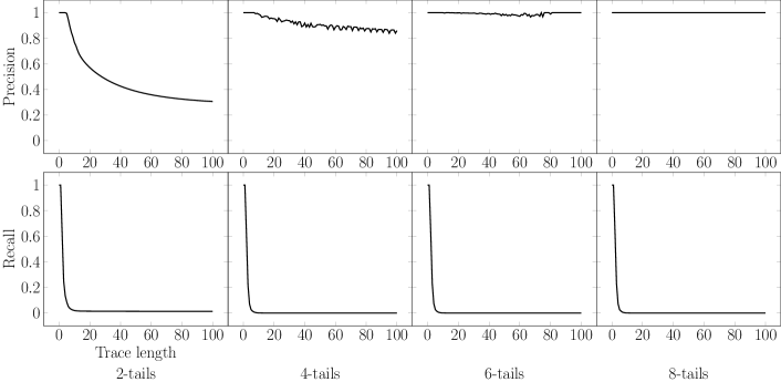
The model accuracy results are summarized in Figure 12, obtained by computing the mean of all the precision values (top row) and recall values (bottom row) for the same trace length ( axis) and the same value of the parameter (2-tails for the leftmost column, 8-tails for the rightmost), across all the test subjects. In accordance with the intuitive summary of -tails presented above, with we obtained inferred models with the highest precision value (equal to 1 across the entire trace length range) but low recall value (less than 0.01 for trace lengths greater than 7). With the precision value is lower (between 1 and 0.28), while the recall value is marginally higher, and stabilizes around 0.012. The fluctuations of the precision values visible for 4-tails and 6-tails are motivated by the fact that for the size of several inferred languages is relatively small (due to the reduced number of merge operations, as highlighted before), resulting in widely variable precision values. The model sizes are summarized in Table 7.
This demonstrates that the trade-off between model size and accuracy that can be achieved by tuning the available parameters of the model inference algorithm used can be rigorously assessed using our proposed method, and shows that in the case of -tails it is consistent with the intuitive understanding of how the algorithm works.
| Min | Avg | Max | |
| 2-tails | 31 | 258 | 907 |
| 4-tails | 53 | 857.8 | 4405 |
| 6-tails | 58 | 1271.9 | 9637 |
| 8-tails | 60 | 1310.6 | 10506 |
Appendix D Appendix: Correlation between model size and model accuracy.
We have investigated whether the state count of the automata accepting the language of false positive and false negatives could be useful as a lightweight proxy to estimate the model accuracy. To do so, we have computed the Pearson correlation coefficient between the cumulative-length model accuracy at different trace lengths, and the state count of and . Since the inference method affects the characteristics of the inferred model, this evaluation was performed separately on the models inferred using k-Tails and MINT.
| MINT | 2-tails | |||||||||
| Trace length | 10 | 20 | 50 | 100 | 200 | 10 | 20 | 50 | 100 | 200 |
| vs. | -0.03 | -0.05 | -0.08 | -0.10 | -0.11 | -0.28 | -0.54 | -0.49 | -0.45 | -0.43 |
| vs. | 0.09 | 0.08 | 0.06 | 0.06 | 0.06 | -0.23 | -0.51 | -0.41 | -0.36 | -0.34 |
| vs. | -0.32 | -0.27 | -0.23 | -0.20 | -0.18 | -0.28 | -0.25 | -0.23 | -0.22 | -0.22 |
| vs. | -0.28 | -0.24 | -0.21 | -0.18 | -0.15 | -0.27 | -0.24 | -0.23 | -0.22 | -0.22 |
The results are summarized in Table 8. Based on the modest measured correlation and its dependence on the inference method used for the model generation, we conclude that the state count of the automata of false positives and false negatives cannot reliably serve as a proxy of the measured accuracy.