ButterflyNet2D: Bridging Classical Methods and Neural Network Methods in Image Processing

Abstract

Both classical Fourier transform-based methods and neural network methods are widely used in image processing tasks. The former has better interpretability, whereas the latter often achieves better performance in practice. This paper introduces ButterflyNet2D, a regular CNN with sparse cross-channel connections. A Fourier initialization strategy for ButterflyNet2D is proposed to approximate Fourier transforms. Numerical experiments validate the accuracy of ButterflyNet2D approximating both the Fourier and the inverse Fourier transforms. Moreover, through four image processing tasks and image datasets, we show that training ButterflyNet2D from Fourier initialization does achieve better performance than random initialized neural networks.

Keywords: Convolutional neural network, ButterflyNet, Butterfly Algorithm, image processing

1 Introduction

Image processing tasks appear widely in our daily life and are handled by classical methods and/or neural network methods behind the screen. Image processing tasks [1] include but are not limited to image denoising, image deblurring, image inpainting, image recognition, image classification, etc. A decade ago, image processing tasks were almost always handled by classical methods, e.g., Fourier transform, wavelet transform, partial differential equations, etc. With the rise of machine learning and neural network, neural network based methods dominate image processing. Among all neural network architecture, deep convolutional neural network (CNN) is the most popular architecture for image processing tasks. Many variants of CNN, including LeNet [2], AlexNet [3], U-Net [4, 5, 6], etc., are proposed and successfully address image processing tasks. In this paper, we bridge the classical method, Fourier transform, with the convolutional neural network method for image processing via ButterflyNet2D.

Fourier transform.

Fourier transform is a linear transformation that decomposes functions into frequency components. It has a wide range of applications in a variety of fields, including signal processing [7, 8], image processing [9, 10, 11], etc. Besides the time-frequency transformation, the existence of the well-known fast algorithm, fast Fourier transform (FFT) [12, 13], makes the transform widely adopted in practice. An FFT decomposes a dense discrete Fourier transform matrix of size $N\times N$ into a product of $O(\log N)$ sparse matrices, each of which is sparsity $O(N)$. Another family of fast algorithms that could be applied to accelerate the Fourier transform is the butterfly algorithm [14, 15, 16, 17, 18, 19]. Although butterfly algorithms were originally designed to accelerate the computation of the Fourier integral operator, they could be applied to approximate the discrete Fourier transform in $O(N\log N)$ operations as well. The same scaling holds for both FFT and butterfly algorithms, while the latter suffers from an approximation error. Hence, for Fourier transform in classical image processing methods, FFT is applied.

Neural Network.

There has been a growing trend to ask for better and faster image processing methods in the last two decades. CNN [2, 20] was initially introduced to process images directly and has later been embedded into other deep neural network architectures [21] to improve image processing further. The success of CNN and its variants in image processing have been demonstrated in tons of works [22, 23]. However, unlike Fourier transform in image processing, which has much mathematical understanding of the methods, CNN lacks interpretability. In most cases, researchers refer to the universal approximation theorem of CNN [24, 25, 26] for its great success in image processing. Recently, the Fourier transform has been imported to be part of the neural network architecture and leads to Fourier CNN [27], Fourier neural network [28], etc. In addition, the FFT structure was incorporated into neural networks and applied to image processing tasks [29, 30]. The connection between the Fourier transform and CNN was established via the butterfly algorithm, and ButterflyNet [26, 31] was proposed to address signal processing tasks and one-dimensional PDEs.

Contribution.

In this work, based on the two-dimensional butterfly algorithm, we introduce a sparsified CNN architecture named ButterFlyNet2D. This neural network with a particular initialization can approximate a two-dimensional discrete Fourier transform. The approximation power is theoretically guaranteed. In summary, our contribution can be organized as follows.

• The ButterflyNet2D network is constructed, which is a CNN architecture with sparse channel connections;

• Fourier initialization is proposed for ButterflyNet2D approximating a two-dimensional discrete Fourier transform with guaranteed approximation error;

• ButterflyNet2D is applied to many ill-posed image processing tasks, i.e., denoising, deblurring, inpainting, and watermark removal, on practical image data sets.

Numerical experiments demonstrate that ButterflyNet2D, as a specialized CNN, along with the Fourier initialization, outperforms its randomly initialized counterpart and another well-known Neumann network [32]. The latter was designed for inverse problems in image processing.

Organization.

The rest paper is organized as follows. Section 2 proposes the ButterflyNet2D architecture and Fourier initialization strategy. In Section 3, ButterflyNet2Ds with Fourier initialization and random initialization are applied to the image denoising, image deblurring, image inpainting, and watermark removal tasks. The comparison against the Neumann network is also presented. Finally, Section 4 concludes the paper.

2 ButterflyNet2D and Fourier Initialization

This section constructs ButterflyNet2D and initializes it as an approximated two-dimensional discrete Fourier transform. We first pave the path to review the two-dimensional butterfly algorithm in Section 2.1. In Section 2.2, the two-dimensional butterfly algorithm is detailed, with the kernel function being Fourier transform. Section 2.3 introduces the architecture of ButterflyNet2D, and its Fourier initialization is proposed in Section 2.4.

2.1 Preliminary

Chebyshev Interpolation.

An important numerical tool in approximating the Fourier transform is the Lagrange polynomial on Chebyshev points, which is known as the Chebyshev interpolation. The Chebyshev points of order $r$ on $[-1/2,1/2]$ are defined as

$$\left\{z_{i}=\frac{1}{2}\cos\frac{(2i-1)\pi}{2r}\right\}_{i\in\{1,\dots,r\}}.$$

The associated Lagrange polynomial at $z_{k}$ admits

$$\mathcal{L}_{k}(x)=\prod_{p\neq k}\frac{x-z_{p}}{z_{k}-z_{p}}.$$

In two dimension, $r^{2}$ Chebyshev points in $[-1/2,1/2]\times[-1/2,1/2]$ are the tensor grid of one-dimensional Chebyshev points,

$$\left\{z_{i,j}=\left(\frac{1}{2}\cos\frac{(2i-1)\pi}{2r},\frac{1}{2}\cos\frac{(2j-1)\pi}{2r}\right)\right\}_{i,j\in\{1,\dots,r\}},$$

The two-dimensional Chebyshev interpolation then admits,

$$\mathcal{L}_{(i,j)}=\mathcal{L}_{i}\mathcal{L}_{j}.$$ (1)

Domain Decomposition.

The butterfly algorithm essentially relies on multiscale domain decomposition. Here we introduce the domain decomposition for square domain pairs. Given two domains $A=[0,K)\times[0,K)$ and $B=[0,1)\times[0,1)$ for $K$ being the frequency range, we conduct 4-partition recursively to both $A$ and $B$. The resulting decomposed domains are denoted as $A_{i_{x},i_{y}}^{\ell}$ and $B_{j_{x},j_{y}}^{L-\ell}$, where $(i_{x},i_{y})$ and $(j_{x},j_{y})$ are indices, and $\ell$ is recursion layer index. More precisely, the explicit expressions of $A_{i_{x},i_{y}}^{\ell}$ and $B_{j_{x},j_{y}}^{L-\ell}$ are

$$\begin{split}A_{i_{x},i_{y}}^{\ell}&=\Bigg{[}\frac{i_{x}K}{2^{\ell+1}},\frac{(i_{x}+1)K}{2^{\ell+1}}\Bigg{)}\times\Bigg{[}\frac{i_{y}K}{2^{\ell+1}},\frac{(i_{y}+1)K}{2^{\ell+1}}\Bigg{)},\\ B_{j_{x},j_{y}}^{L-\ell}&=\Bigg{[}\frac{j_{x}}{2^{L-\ell-1}},\frac{(j_{x}+1)}{2^{L-\ell-1}}\Bigg{)}\times\Bigg{[}\frac{j_{y}}{2^{L-\ell-1}},\frac{(j_{y}+1)}{2^{L-\ell-1}}\Bigg{)}.\end{split}$$

Figure 1 gives a 3-layer recursive domain decomposition example.

Figure 1: Recursive domain decomposition for $A,B$.

We further adopt the notation $\prec$ to denote the relationship among recursive partitions, i.e., $(\tilde{i}_{x},\tilde{i}_{y})\prec(i_{x},i_{y})$ or $A_{\tilde{i}_{x},\tilde{i}_{y}}^{\ell+1}\prec A_{i_{x},i_{y}}^{\ell}$ means that

$$A_{\tilde{i}_{x},\tilde{i}_{y}}^{\ell+1}\subset A_{i_{x},i_{y}}^{\ell}$$

for some $\ell$. Similarly, $(j_{x},j_{y})\prec(\tilde{j}_{x},\tilde{j}_{y})$, or $B_{j_{x},j_{y}}^{L-\ell}\prec B_{\tilde{j}_{x},\tilde{j}_{y}}^{L-\ell-1}$, means

$$B_{j_{x},j_{y}}^{L-\ell}\subset B_{\tilde{j}_{x},\tilde{j}_{y}}^{L-\ell-1}$$

for some $\ell$. The layer index $\ell$ in all cases can be referred from the text around. As in Figure 1, we have

$$\begin{split}B_{00}^{2}\prec B_{00}^{1}\prec B_{00}^{0},\\ A_{00}^{2}\prec A_{00}^{1}\prec A_{00}^{0}.\end{split}$$

Low-Rank Approximation of Fourier Kernel.

The Fourier kernel,

$$\mathcal{K}(\xi,t)=e^{-2\pi\imath\xi\cdot t},\quad\xi\in[0,K)\times[0,K)\text{ and }t\in[0,1)\times[0,1),$$

is a Fourier integral operator. Different from general multi-dimensional Fourier integral operator, the Fourier kernel does not have a singularity around the origin. Hence the low-rank approximation theorem for one-dimensional Fourier integral operator could be extended to the two-dimensional Fourier kernel.

Theorem 2.1.

Let $A\subset[0,K)^{2}$ and $B\subset[0,1)^{2}$ be a domain pair such that $\gamma=\frac{e\pi\omega(A)\omega(B)}{r^{2}}<1$ , where $r^{2}$ is the number of Chebyshev points. Then the Fourier kernel restricted to the domain pair admits both low-rank approximations,

$$\begin{split}\sup_{\xi\in A,t\in B}\left|e^{-2\pi\imath\xi\cdot t}-\sum_{k_{x}=1}^{r}\sum_{k_{y}=1}^{r}e^{-2\pi\imath\xi\cdot t_{k_{x},k_{y}}}e^{-2\pi\imath\xi_{0}\cdot(t-t_{k_{x},k_{y}})}\mathcal{L}_{k_{x},k_{y}}(t)\right|\leq&C\frac{\gamma^{r^{2}}}{1-\gamma},\text{ and}\\ \sup_{\xi\in A,t\in B}\left|e^{-2\pi\imath\xi\cdot t}-\sum_{k_{x}=1}^{r}\sum_{k_{y}=1}^{r}\mathcal{L}_{k_{x},k_{y}}(\xi)e^{-2\pi\imath(\xi-\xi_{k})\cdot t_{0}}e^{-2\pi\imath\xi_{k_{x},k_{y}}\cdot t}\right|\leq&C\frac{\gamma^{r^{2}}}{1-\gamma},\end{split}$$

where $\xi_{0}$ and $t_{0}$ are centers of $A$ and $B$ respectively, $C$ is a constant independent of $t$ and $\xi$, $\xi_{k_{x},k_{y}}$ and $t_{k_{x},k_{y}}$ are Chebyshev points on $A$ and $B$.

A sketched proof of Theorem 2.1 can be found in Appendix 5.1. From Theorem 2.1, when restricted to the desired domain pairs, the Fourier kernel can be well-approximated by a low-rank factorization. An underlying matrix-vector multiplication can be approximated as,

$$\begin{split}u^{B}(\xi)=\sum_{t\in B}K(\xi,t)x(t)\approx&\sum_{k_{x}=1}^{r}\sum_{k_{y}=1}^{r}\alpha_{k_{x},k_{y}}(\xi)\left(\sum_{t\in B}\beta_{k_{x},k_{y}}(t)x(t)\right)\\ =&\sum_{k_{x}=1}^{r}\sum_{k_{y}=1}^{r}\alpha_{k_{x},k_{y}}(\xi)\lambda_{k_{x},k_{y}}^{AB},\end{split}$$ (2)

where

$$\begin{split}\alpha_{k_{x},k_{y}}(\xi)=&e^{-2\pi\imath\xi\cdot t_{k_{x},k_{y}}},\\ \beta_{k_{x},k_{y}}(t)=&e^{-2\pi\imath\xi_{0}\cdot(t-t_{k_{x},k_{y}})}\mathcal{L}_{k_{x},k_{y}}(t),\text{ and}\\ \lambda_{k_{x},k_{y}}^{AB}=&\sum_{t\in B}\beta_{k_{x},k_{y}}(t)x(t).\end{split}$$

Hence, the Fourier transform of the vector $x(t)$ is turned into computing $\lambda_{k_{x},k_{y}}^{AB}$. The butterfly algorithm employs (2) recursively to reduce the quadratic computational cost down to quasi-linear.

2.2 2D Butterfly Algorithm Revisit

We revisit the butterfly algorithm applying to the two-dimensional Fourier kernel. We first conduct a $L$-layer recursive domain decomposition for both $A^{0}_{00}=[0,K)^{2}$ and $B^{0}_{00}=[0,1)^{2}$. The butterfly algorithm comprises three major steps: interpolation at $\ell=0$, recursion, and kernel application at $\ell=L$. The interpolation at $\ell=0$ interpolates function on a uniform grid in $B^{0}_{00}$ to Chebyshev grids on $B^{L}_{j_{x},j_{y}}$ for all $(j_{x},j_{y})$. The recursion step then recursively interpolates the function on four Chebyshev grids at the finer domain layer to the Chebyshev grid at the coarse domain layer. Finally, the kernel application step applies the Fourier kernel. The 2D butterfly algorithm applying to the Fourier kernel is detailed as follows.

1. Interpolation ($\ell=0$). For each domain pair $(A_{i_{x},i_{y}}^{0},B_{j_{x},j_{y}}^{L})$ at layer $\ell=0$, $i_{x},i_{y}\in[2],j_{x},j_{y}\in[2^{L-1}]$ , we conduct a coefficient transfer from the uniform grid in $B_{j_{x},j_{y}}^{L}$ to Chebyshev points in the same domain. The constructed expansion coefficients admit,

   $$\lambda_{t_{(k_{x},k_{y})}}^{A_{i_{x},i_{y}}^{0}B_{j_{x},j_{y}}^{L}}=\sum_{t_{\text{uni}}\in B_{j_{x},j_{y}}^{L}}e^{-2\pi\imath\xi_{0}^{i_{x},i_{y}}\cdot(t_{\text{uni}}-t_{(k_{x},k_{y})})}\mathcal{L}_{(k_{x},k_{y})}(t_{\text{uni}})x(t_{\text{uni}}),$$ (3)

   for $t_{(k_{x},k_{y})}\in B_{j_{x},j_{y}}^{L}$ being the Chebyshev points therein and $\xi_{0}^{i_{x},i_{y}}$ being the center of $A_{i_{x},i_{y}}^{0}$. Throughout the paper, we add a subscript “uni” to indicate the uniform grid point in the domain, e.g., $t_{\text{uni}}\in B^{L}_{j_{x},j_{y}}$ denotes the uniform grid points in $B^{L}_{j_{x},j_{y}}$.

2. Recursion($\ell=1,\dots,L-1$). For each domain pair ($A_{i_{x},i_{y}}^{\ell-1}$, $B_{j_{x},j_{y}}^{L-\ell+1}$), $i_{x},i_{y}\in[2^{\ell}]$, $j_{x},j_{y}\in[2^{L-\ell}]$, we conduct coefficients transfer from the Chebyshev points in $B_{j_{x},j_{y}}^{L-\ell+1}$ to the Chebyshev points in $B_{\tilde{j}_{x},\tilde{j}_{y}}^{L-\ell}$. The domain $B_{\tilde{j}_{x},\tilde{j}_{y}}^{L-\ell}$ is a parent domain of $B_{j_{x},j_{y}}^{L-\ell+1}$, i.e., $B_{j_{x},j_{y}}^{L-\ell+1}\prec B_{\tilde{j}_{x},\tilde{j}_{y}}^{L-\ell}$. Similarly, the other domain satisfies $A_{\tilde{i}_{x},\tilde{i}_{y}}^{\ell}\prec A_{i_{x},i_{y}}^{\ell-1}$. The coefficients transfer admits,

   $$\lambda_{t_{(k_{x},k_{y})}}^{A_{\tilde{i}_{x},\tilde{i}_{y}}^{\ell}B_{\tilde{j}_{x},\tilde{j}_{y}}^{L-\ell}}=\sum_{(j_{x},j_{y})\prec(\tilde{j}_{x},\tilde{j}_{y})}\sum_{t\in B_{j_{x},j_{y}}^{L-\ell+1}}e^{-2\pi\imath\xi_{0}\cdot(t-t_{(k_{x},k_{y})})}\mathcal{L}_{(k_{x},k_{y})}(t)\lambda_{t}^{A_{i_{x},i_{y}}^{\ell-1}B_{j_{x},j_{y}}^{L-\ell+1}},$$ (4)

   for $t_{(k_{x},k_{y})}\in B_{j_{x},j_{y}}^{L-\ell}$ and $(\tilde{i}_{x},\tilde{i}_{y})\prec(i_{x},i_{y})$, where $t$ and $t_{(k_{x},k_{y})}$ are Chebyshev points in $B_{j_{x},j_{y}}^{L-\ell+1}$ and $B_{\tilde{j}_{x},\tilde{j}_{y}}^{L-\ell}$ respectively, $\xi_{0}$ is the center of $A_{\tilde{i}_{x},\tilde{i}_{y}}^{l}$.

3. Kernel Application($\ell=L$). In the last step, the domain pairs are ($A_{i_{x},i_{y}}^{L}$, $B_{0,0}^{0}$) for $i_{x},i_{y}\in[2^{L}]$. All previous layers are transferring coefficients via interpolation. This step applies the Fourier kernel to the transferred coefficients, and approximate $u(\xi)$ as

   $$u(\xi_{\text{uni}})\approx\sum_{t_{(k_{x},k_{y})}\in B_{0,0}^{0}}e^{-2\pi\imath\xi_{\text{uni}}\cdot t_{(k_{x},k_{y})}}\lambda_{t_{(k_{x},k_{y})}}^{A_{i_{x},i_{y}}^{L}B_{0,0}^{0}},$$ (5)

   for $\xi_{\text{uni}}$ being uniform grids in $A_{i_{x},i_{y}}^{L}$. This gives us the desired approximation of $u(\xi)$.

Butterfly algorithm, in general, carries a complicated procedure. In this revisit, we omit most intuition behind operations and review the algorithm flow. For more details, readers are referred to [26].

2.3 ButterflyNet2D

This section introduces the network architecture of ButterflyNet2D, which is a CNN architecture with sparsely connected channels. In the revisit of the butterfly algorithm, we make a crucial observation that the summation kernels in (3) and (4) are independent of the subdomain $B^{\ell}_{j_{x},j_{y}}$. More precisely, the summation kernels in (3) and (4),

$$e^{-2\pi\imath\xi_{0}^{i_{x},i_{y}}\cdot(t_{\text{uni}}-t_{(k_{x},k_{y})})}\mathcal{L}_{(k_{x},k_{y})}(t_{\text{uni}})\quad\text{and}\quad e^{-2\pi\imath\xi_{0}\cdot(t-t_{(k_{x},k_{y})})}\mathcal{L}_{(k_{x},k_{y})}(t).$$

depend only on the relative distance of either $t_{\text{uni}}$ and $t_{(k_{x},k_{y})}$ or $t$ and $t_{(k_{x},k_{y})}$. Therefore, these two summation kernels are the same for all $B^{\ell}_{j_{x},j_{y}}$ at the same $\ell$-layer. The summations as in (3) and (4) are convolutions and could be represented by a CNN. In the following, we construct the ButterflyNet2D architecture, which mimics the structure of the butterfly algorithm and replace the summation operations by convolutions.

Network Architecture.

We introduce the construction of a ButterflyNet2D with $L$ layers. The input is denoted as $Z^{(0)}$, whose size is $\omega_{x}2^{L-1}\times\omega_{y}2^{L-1}$ and channel size is 1. The generalization to inputs of other sizes is straightforward. We adopt a channel-first index rule, i.e., the input is indexed as $Z^{0}(c,i,j)$, where $c=0$ is the channel index, $i$ and $j$ range from $0$ to $\omega_{x}2^{L-1}-1$ and $\omega_{y}2^{L-1}-1$ respectively are two spacial indices. The desired output is assumed to be of size $m_{x}2^{L}\times m_{y}2^{L}$. The network architecture could then be constructed as follows.

1. Interpolation($\ell=0$). Given $c\in[4r^{2}]$, the first layer is described as

   $$Z^{(1)}(c,i,j)=\sigma\left\{B^{(0)}(c)+\sum_{\begin{subarray}{c}s_{x}\in[\omega_{x}]\\ s_{y}\in[\omega_{y}]\end{subarray}}W^{(0)}(0,c,s_{x},s_{y})Z^{(0)}(0,\omega_{x}i+s_{x},\omega_{y}j+s_{y})\right\},$$ (6)

   for $i$, $j=[2^{L-1}]$, where $\sigma\{\cdot\}$ is the nonlinear ReLU activation function, $B^{(0)}$ is the bias, $W^{(0)}$ is the convolution kernel. The output function at the current layer has $4r^{2}$ channels. This layer is a regular 2D convolution layer with input sizes $\omega_{x}2^{L-1}\times\omega_{y}2^{L-1}$, input channel size 1, output channel size $4r^{2}$, convolution kernel size $\omega_{x}\times\omega_{y}$, stride $(\omega_{x},\omega_{y})$.

2. Recursion($\ell=1,\dots,L-1$). The input at the $\ell$ layer is of size $2^{L-\ell}\times 2^{L-\ell}$ and channel size $4^{\ell}r^{2}$. The convolution operation at the current layer admits,

   $$Z^{(\ell+1)}(c_{\text{o}},i,j)=\sigma\left\{B^{(\ell)}(c_{\text{o}})+\sum_{\begin{subarray}{c}kr^{2}\leq c_{\text{i}}<(k+1)r^{2}\\ s_{x},s_{y}\in[2]\end{subarray}}W^{(\ell)}(c_{\text{i}},c_{\text{o}},s_{x},s_{y})Z^{(\ell)}(c_{\text{i}},2i+s_{x},2j+s_{y})\right\},$$ (7)

   where $i,j=[2^{L-\ell-1}]$, $c_{\text{o}}\in[4^{\ell+1}r^{2}]$, and $k=c_{\text{o}}/(4r^{2})$. We notice the relation $(\tilde{i}_{x},\tilde{i}_{y})\prec(i_{x},i_{y})$ in (4). Hence in our network architecture, different from the regular fully connected channel 2D convolutional layer, the input channels and output channels in (7) are sparsely connected. We could also view (7) as a sequence of $4^{\ell}$ regular 2D convolutional layers with input size $2^{L-\ell}\times 2^{L-\ell}$, output size $2^{L-\ell-1}\times 2^{L-\ell-1}$, input channel size $r^{2}$, and output channel size $4r^{2}$, acting to each set of input channels and then concatenate the output along the channel direction.

3. Kernel Application($\ell=L$). There are two ways to view the kernel application layer. From the convolutional layer point of view, we apply 2D convolutional layers with sparse channel connection, where the input size is $1\times 1$. From a dense layer point of view, we apply a dense layer to each set of channels in the input. From either point of view, we could represent the operation as,

   $$Z^{(L+1)}(c_{\text{o}},0,0)=\sigma\left\{B^{(L)}(c_{\text{o}})+\sum_{kr^{2}\leq c_{\text{i}}<(k+1)r^{2}}W^{(L)}(c_{\text{i}},c_{\text{o}},0,0)Z^{(L)}(c_{\text{i}},0,0)\right\},$$ (8)

   where $c_{\text{o}}\in[m_{x}m_{y}4^{L}]$.

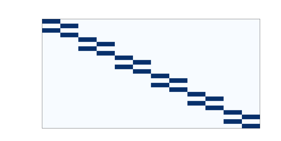
Figure 2: Input and output channel connection in ButterflyNet2D.

An important difference between the ButterflyNet2D and regular 2D CNN is the connectivity between input and output channels. ButterflyNet2D has a sparse channel connection, whereas a regular 2D CNN has a dense connection between input and output channels. Figure 2 offers an illustration for the channel connections in ButterflyNet2D.

Parameter Counting.

For a ButterflyNet2D with $L$ layers and $r^{2}$ Chebyshev grid points, the input and output are assumed to be of size $\omega_{x}2^{L-1}\times\omega_{y}2^{L-1}$ and $m_{x}2^{L}\times m_{y}2^{L}$ respectively. We calculate the number of convolutional kernel weights and bias weights. As been explained in Appendix 5.2, all weights and bias in (6), (7), and (8), are $4\times 4$ real matrices, which would then be initialized to approximate the complex numbers for Fourier transform. The calculation for the number of weights is as follows.

1. Interpolation($\ell=0$). The number of nonzeros in the convolution kernel $W^{(0)}$ is

   $$\mathrm{nnz}(W^{(0)})=4\times(4\times 4\times r^{2})\times(\omega_{x}\times\omega_{y})=4^{3}r^{2}\omega_{x}\omega_{y},$$

   whereas that in the bias $B^{(0)}$ is

   $$\mathrm{nnz}(B^{(0)})=4\times(4\times r^{2})=4^{2}r^{2}.$$

2. Recursion($\ell=1,\dots,L-1$). The number of nonzeros in the convolution kernel $W^{(\ell)}$ is

   $$\mathrm{nnz}(W^{(\ell)})=4^{\ell}\times(4\times r^{2})\times(4\times 4\times r^{2})\times(2\times 2)=4^{\ell+4}r^{4},$$

   whereas that in the bias $B^{(\ell)}$ is

   $$\mathrm{nnz}(B^{(\ell)})=4^{\ell}\times(4\times 4\times r^{2})=4^{\ell+2}r^{2}.$$

   Hence summing over all layers, the total number of weights in convolution kernel and bias in the recursion step admits,

   $$\sum_{\ell=1}^{L-1}\mathrm{nnz}(W^{(\ell)})=\frac{4^{L+4}-4^{5}}{3}r^{4},\quad\sum_{\ell=1}^{L-1}\mathrm{nnz}(B^{(\ell)})=\frac{4^{L+2}-4^{3}}{3}r^{2}.$$

3. Kernel Application($\ell=L$). The number of nonzeros in the convolution kernel $W^{(L)}$ is

   $$\mathrm{nnz}(W^{(\ell)})=4^{L}\times(4\times r^{2})\times(4\times m_{x}\times m_{y})\times(1\times 1)=4^{L+2}r^{2}m_{x}m_{y},$$

   whereas that in the bias $B^{(L)}$ is

   $$\mathrm{nnz}(B^{(L)})=4^{L}\times(4\times m_{x}\times m_{y})=4^{L+1}m_{x}m_{y}.$$

With an input that is of the size $N\times N$, the number of layers in the network could be $L=\log N$. The overall number of weights is

$$4^{2}r^{2}(1+4\omega_{x}\omega_{y})+\frac{4^{L+2}-4^{3}}{3}r^{2}(1+4^{2}r^{2})+4^{L+1}m_{x}m_{y}(1+4r^{2})=O(N).$$

When a similar CNN is considered and channels are fully connected, the number of weights would be

$$4^{2}r^{2}(1+4\omega_{x}\omega_{y})+\frac{4^{L+2}-4^{3}}{3}+\frac{4^{2L+8}-4^{6}}{15}+4^{L+1}m_{x}m_{y}(1+4r^{2})=O(N^{2}+N).$$

Hence, ButterflyNet2D, compared to the regular CNN, reduces the number of weights by a factor of $O(N)$.

2.4 Fourier Initialization

The ButterflyNet2D is constructed in a way mimicking the butterfly algorithm. Extra bias weights and ReLU activation functions are added. We now propose an initialization strategy, which transfers coefficients in the butterfly algorithm to convolution kernels in ButterflyNet2D. Given the same input and output sizes, and the same number of Chebyshev points, when the initialization strategy is applied, the ButterflyNet2D is identical to the butterfly algorithm. We adopt a re-indexing of the channel,

$$c=(i_{x},i_{y},k_{x},k_{y})$$

for subdomain $A_{i_{x},i_{y}}^{\ell}$ and the Chebyshev node index $(k_{x},k_{y})$. In the initialization strategy, named Fourier initialization, all bias weights are initialized to be zero. The convolution kernel weights are initialized as follows, where complex coefficients are converted to $4\times 4$ matrixes as in Appendix 5.2.

1. Interpolation($\ell=0$). Since the summation in (3) is a convolution, the dependence on $B^{(L)}_{j_{x},j_{y}}$ could be ignored. We initialize the convolution kernel $W^{(0)}$ as,

   $$W^{(0)}(0,c,s_{x},s_{y})=e^{-2\pi\imath\xi_{0}^{i_{x},i_{y}}\cdot(u_{(s_{x},s_{y})}-t_{(k_{x},k_{y})})}\mathcal{L}_{(k_{x},k_{y})}(u_{(s_{x},s_{y})}),$$

   where $u_{(s_{x},s_{y})}$ and $t_{(k_{x},k_{y})}$ are the uniform grid and Chebyshev grid in $B_{0,0}^{L}$ respectively.

2. Recursion($\ell=1,\dots,L-1$). The summation in (4) is a convolution with a sparse channel connection, the dependence on $B^{(L-\ell+1)}_{j_{x},j_{y}}$ could be ignored. We initialize the convolution kernel $W^{(\ell)}$ as

   $$W^{(\ell)}(c_{\text{i}},c_{\text{o}},s_{x},s_{y})=e^{-2\pi\imath\xi_{0}\cdot(u_{(s_{x},s_{y})}-t_{(k_{x},k_{y})})}\mathcal{L}_{(k_{x},k_{y})}(u_{(s_{x},s_{y})}),$$

   where $u_{(s_{x},s_{y})}$ is the Chebyshev node in $B_{j_{x},j_{y}}^{L-\ell+1}$, where $j_{x}\in[2],j_{y}\in[2]$. And $t_{(k_{x},k_{y})}$ is the Chebyshev node in $B_{0,0}^{L-\ell}$. Importantly, the input and output channel indices $c_{\text{i}}$ and $c_{\text{o}}$ are re-indexed as $(i_{x},i_{y},s_{x},s_{y})$ and $(\tilde{i}_{x},\tilde{i}_{y},k_{x},k_{y})$, such that $A_{\tilde{i}_{x},\tilde{i}_{y}}^{\ell+1}\prec A_{i_{x},i_{y}}^{\ell}$.

3. Kernel Application($\ell=L$). For the domain pair $(A_{i_{x},i_{y}}^{L},B_{0,0}^{0})$, the kernel weights connects (5) and (8) as,

   $$W^{(L+1)}(c_{\text{i}},c_{\text{o}},0,0)=e^{-2\pi\imath\xi_{(k_{x},k_{y})}\cdot(t_{(s_{x},s_{y})})},$$

   where $t_{(s_{x},s_{y})}$ is the Chebyshev node in $B_{0,0}^{0}$ and $\xi_{(k_{x},k_{y})}$ is the uniform grid in $A_{i_{x},i_{y}}^{L}$.

Both the Fourier kernel and the inverse Fourier kernel admit the low-rank approximation property in Theorem 2.1. Hence, we could also initialize the ButterflyNet2D to approximate the inverse Fourier transform. The initialization detail is omitted. Instead, we numerically demonstrate the performance in the next section.

3 Numerical Experiments

We implemented ButterflyNet2D together with random and Fourier initialization in Python, with PyTorch (1.11.0). The code is available at https://github.com/Genz17/ButterFlyNet2D. In Section 3.1, we first apply the ButterflyNet2D to approximate the Fourier transform and inverse Fourier transform to verify the approximation accuracy of the Fourier initialization. Then in Section 3.2, several image processing tasks on practical image datasets are addressed by ButterflyNet2D.

3.1 Approximation of Fourier Transform

We explore the approximation power of Fourier initialization for the ButterflyNet2D before and after training. The approximation power is measured by the relative matrix norm,

$$\epsilon_{p}:=\frac{\|\mathcal{B}-\mathcal{F}\|_{p}}{\|\mathcal{F}\|_{p}},$$

where $\mathcal{B}$, $\mathcal{F}$ denote the matrix representation of ButterflyNet2D and discrete (inverse) Fourier transform matrix, respectively.

Approximation Before Training.

We apply ButterflyNet2D with Fourier initialization to both the Fourier transform and inverse Fourier transform with $N=64\times 64$. The numerical results are included in Table 1 and Table 2.

	layer $L$ (with $r=6$)			Cheb $r^{2}$ (with $L=6$)
	4	5	6	$4^{2}$	$5^{2}$	$6^{2}$
$\epsilon_{1}$	$5.27\times 10^{-1}$	$3.64\times 10^{-2}$	$1.72\times 10^{-3}$	$5.30\times 10^{-2}$	$8.18\times 10^{-3}$	$1.72\times 10^{-3}$
$\epsilon_{2}$	$7.71\times 10^{-1}$	$6.05\times 10^{-1}$	$1.84\times 10^{-3}$	$8.20\times 10^{-2}$	$1.20\times 10^{-2}$	$1.84\times 10^{-3}$
$\epsilon_{\infty}$	$8.07\times 10^{0}$	$3.73\times 10^{-2}$	$1.12\times 10^{-3}$	$6.65\times 10^{-2}$	$8.16\times 10^{-3}$	$1.12\times 10^{-3}$

Table 1: ButterflyNet2D with Fourier initialization approximating Fourier transform with $N=64\times 64$ before training.

	layer $L$ (with $r=6$)			Cheb $r^{2}$ (with $L=6$)
	4	5	6	$4^{2}$	$5^{2}$	$6^{2}$
$\epsilon_{1}$	$9.04\times 10^{-1}$	$6.80\times 10^{-2}$	$3.07\times 10^{-3}$	$1.07\times 10^{-1}$	$1.89\times 10^{-2}$	$3.07\times 10^{-3}$
$\epsilon_{2}$	$1.16\times 10^{0}$	$7.87\times 10^{-2}$	$3.10\times 10^{-3}$	$1.09\times 10^{-1}$	$1.89\times 10^{-2}$	$3.10\times 10^{-3}$
$\epsilon_{\infty}$	$4.19\times 10^{0}$	$1.76\times 10^{-1}$	$4.83\times 10^{-3}$	$1.79\times 10^{-1}$	$3.03\times 10^{-2}$	$4.83\times 10^{-3}$

Table 2: ButterflyNet2D with Fourier initialization approximating inverse Fourier transform with $N=64\times 64$ before training.

From both Table 1 and Table 2, the relative error decays exponentially with respect to both the layer number $L$ and the number of Chebyshev points $r^{2}$.

Approximation After Training.

We further train ButterflyNet2D with Fourier initialization in approximating the Fourier transform and inverse Fourier transform with $N=64\times 64$. The training data is generated by the exact Fourier and inverse Fourier transforms with uniform random input vectors. The loss function is the $\ell_{2}$ relative error. For training, we adopt Adam optimizer with a learning rate $0.001$ and batch size of 20. The numerical results after 200 epochs are included in Table 3 and Table 4.

	layer $L$ (with $r=6$)		Cheb $r^{2}$ (with $L=6$)
	3	4	$2^{2}$	$3^{2}$
$\epsilon_{1}$	$9.51\times 10^{-1}$	$2.78\times 10^{-1}$	$3.66\times 10^{-1}$	$6.49\times 10^{-2}$
$\epsilon_{2}$	$4.96\times 10^{-1}$	$1.64\times 10^{-1}$	$1.97\times 10^{-1}$	$3.74\times 10^{-2}$
$\epsilon_{\infty}$	$2.58\times 10^{-2}$	$2.08\times 10^{-2}$	$1.93\times 10^{-2}$	$8.54\times 10^{-3}$

Table 3: ButterflyNet2D with Fourier initialization approximating Fourier transform with $N=64\times 64$ after training.

	layer $L$ (with $r=6$)		Cheb $r^{2}$ (with $L=6$)
	3	4	$2^{2}$	$3^{2}$
$\epsilon_{1}$	$5.00\times 10^{-1}$	$1.39\times 10^{-1}$	$2.42\times 10^{-1}$	$3.32\times 10^{-2}$
$\epsilon_{2}$	$5.02\times 10^{-1}$	$1.60\times 10^{-1}$	$2.62\times 10^{-1}$	$3.60\times 10^{-2}$
$\epsilon_{\infty}$	$7.04\times 10^{-1}$	$5.04\times 10^{-1}$	$5.45\times 10^{-1}$	$1.03\times 10^{-1}$

Table 4: ButterflyNet2D with Fourier initialization approximating inverse Fourier transforms with $N=64\times 64$ after training.

Comparing Table 1 and Table 3, we find that training a Fourier initialized ButterflyNet2D could further improve the approximation accuracy. ButterflyNet2D with smaller $r^{2}$ after training achieves better accuracy than the network with larger $r^{2}$ without training. A similar conclusion holds for inverse Fourier transform if we compare Table 2 and Table 4. We further include the training result for ButterflyNet2D with Kaiming random initialization in Appendix 5.3. If we compare the training result for Fourier initialization and Kaiming random initialization, we find that ButterFlyNet2D with Fourier initialization achieves better accuracy in approximating Fourier and inverse Fourier transform.

3.2 Image Processing Tasks

We apply ButterflyNet2D to four major image processing tasks: inpainting, deblurring, denoising, and watermark removal. For the inpainting task, we adopt a $10\times 10$ mask for $32\times 32$ pictures, and when the picture size doubles, the mask size doubles. For example, a mask of the size $80\times 80$ is applied to input pictures of size $256\times 256$. For the deblurring task, the blurring kernel is a $5\times 5$ Gaussian kernel with a standard deviation of $2.5$. For the denoising task, we add Gaussian noise with mean zero and standard deviation $0.1$. We add $8$ horizontal and vertical black lines to the original input picture for the watermark removal task. The line width increases with the picture size. Three picture datasets used are CIFAR10, STL10, and CelebA. They contain 30000, 5000, 30000 pictures, respectively. For testing purposes, we resize pictures into different sizes. We crop the pictures into $2\times 2$ or $4\times 4$ parts to make the neural network more efficient.

The neural network is not the vanilla ButterflyNet2D. We adopt the idea of special-frequence transformation property and construct the neural network architecture to be a ButterflyNet2D applied after another ButterflyNet2D, named ButterflyNet2D². Both ButterflyNet2Ds have $\log_{2}(\text{Input Size})$ layers and $2^{2}$ Chebyshev points. The first ButterflyNet2D is initialized to approximate the Fourier transform, whereas the second one is initialized to approximate the inverse Fourier transform. Hence the neural network is initialized as an approximation of the identity mapping.

Relative vector 2-norm error is used as the loss function,

$$\mathcal{L}=\sum_{i=1}^{N}\frac{\|\mathcal{B}(x_{i})-x_{i}\|_{2}}{\|x_{i}\|_{2}},$$

where $\mathcal{B}$ denotes the neural network and $x_{i}$ is the $i$-th training data out of $N$ pictures. The PSNR with a batch size of 256 is used as the measurement of testing results,

$$\text{PSNR}=\frac{\sum_{x\in\text{Batch}}-10\log_{10}\left(\|\mathcal{B}(x)-x\|_{2}^{2}/(3S_{x}S_{y})\right)}{\text{Batch Size}},$$ (9)

where $\mathcal{B}(x)$ and $x$ are RGB-colored pictures whose sizes are $S_{x}\times S_{y}$. Adam optimizer with an initial learning rate of $2\times 10^{-3}$ is adopted as the minimizer. Further, “ReduceLROnPlateau” learning rate decay strategy is applied with a factor of 0.98 and patience of 100. All the details of epochs and batch sizes are shown in Table 5.

Task	Dataset	Input Size	Training Epochs	Batch Size
Inpainting Denoising Deblurring	CelebA($64\times 64$)	$32\times 32$	12	20
	CelebA($128\times 128$)	$64\times 64$	12	20
	CelebA($256\times 256$)	$64\times 64$	3	5
	CIFAR10($32\times 32$)	$32\times 32$	12	20
	STL10($64\times 64$)	$32\times 32$	72	20
Watermark Removal	CelebA($64\times 64$)	$16\times 16$	3	5
	CelebA($128\times 128$)	$32\times 32$	3	5
	CelebA($256\times 256$)	$32\times 32$	3	5
	CIFAR10($32\times 32$)	$16\times 16$	12	20
	STL10($64\times 64$)	$16\times 16$	12	5

Table 5: Batch sizes and epochs for various tasks on various datasets.

All the pictures in the datasets are RGB-colored pictures. We turn them into grayscale for training. Then the trained ButterflyNet2D² is applied to each of the three color channels of testing pictures. The three outputs are concatenated along the channel direction and form an RGB-colored picture.

		Initialization
Task	Dataset	Fourier	Uniform	Normal
Inpaint	CelebA($64\times 64$)	$30.25$	$16.51$	$17.39$
	CelebA($128\times 128$)	$30.55$	$17.91$	$18.39$
	CelebA($256\times 256$)	$30.83$	$17.63$	$18.49$
	CIFAR10($32\times 32$)	$28.73$	$15.97$	$17.23$
	STL10($64\times 64$)	$25.77$	$16.03$	$16.87$
Deblur	CelebA($64\times 64$)	$36.27$	$16.16$	$17.27$
	CelebA($128\times 128$)	$38.30$	$17.93$	$18.02$
	CelebA($256\times 256$)	$43.30$	$17.60$	$17.49$
	CIFAR10($32\times 32$)	$40.39$	$16.35$	$17.14$
	STL10($64\times 64$)	$33.88$	$16.16$	$16.99$
Denoise	CelebA($64\times 64$)	$26.71$	$16.18$	$17.55$
	CelebA($128\times 128$)	$29.07$	$17.30$	$18.15$
	CelebA($256\times 256$)	$32.02$	$18.17$	$18.59$
	CIFAR10($32\times 32$)	$26.33$	$16.38$	$16.57$
	STL10($64\times 64$)	$26.57$	$15.40$	$17.10$
Watermark Removal	CelebA($64\times 64$)	$31.63$	$18.25$	$18.02$
	CelebA($128\times 128$)	$35.14$	$16.02$	$17.18$
	CelebA($256\times 256$)	$41.69$	$16.03$	$17.31$
	CIFAR10($32\times 32$)	$31.13$	$17.00$	$16.08$
	STL10($64\times 64$)	$32.29$	$17.48$	$17.54$

Table 6: The numerical results of ButterflyNet2D².

Figure 3: Original picture, distorted picture, and recovered picture by ButterflyNet2D². From top to bottom, the distortions are inpainting, denoising, deblurring, and watermark removal. From left to right, the datasets are CelebA, CIFAR10 and STL10.

Task	Dataset	Preconditioned	Not Preconditioned
Inpaint	CelebA($64\times 64$)	30.45	31.06
	CIFAR10($32\times 32$)	28.40	28.20
	STL10($64\times 64$)	28.00	27.47
Deblur	CelebA($64\times 64$)	33.79	31.01
	CIFAR10($32\times 32$)	37.83	36.55
	STL10($64\times 64$)	30.66	29.43

Table 7: The numerical results of Neumann network.

Table 6 and Figure 3 illustrates all numerical results of ButterflyNet2D² applying to various tasks and datasets. According to Table 6, the Fourier initialization outperforms both Kaiming uniform random initialization and Kaiming normal random initialization. As the complexity of the neural network increases, the training becomes more difficult. The Fourier initialization bridges the classical image processing method with the neural network methods. The network training starts from the classical method and approaches the benefit of neural networks. We make another comparison against Neumann network. In the inpainting tasks, ButterflyNet2D² and Neumann network perform similarly. While in the deblurring tasks, ButterflyNet2D² with Fourier initialization outperforms Neumann Network. This result is not surprising since deblurring is easier in the frequency domain.

4 Conclusions and Discussions

In this paper, we proposed a neural network architecture named ButterflyNet2D, together with a specially designed Fourier initialization. The ButterflyNet2D with Fourier initialization approximates discrete Fourier transforms with $O(N)$ parameters, where $N$ is the input size. ButterflyNet2D and Fourier initialization allow us to bridge the classical Fourier transformation method and powerful neural network methods for image processing tasks.

Through numerical experiments, we explored the approximation power of ButterflyNet2D with Fourier initialization before and after training. Numerical results show that ButterflyNet2D with Fourier initialization well-approximates the Fourier transform and the training could further improve the approximation accuracy. Tests of ill-posed image processing tasks are also conducted. ButterflyNet2D shows its power in these tasks.

The work can be extended in several directions. Firstly, the initialization method has limited versatility. The Fourier initialization method heavily relies on the ButterflyNet2D architecture. Many popular techiniques, e.g., max-pooling, batch normalization, or dropout, currently cannot be incorporated with the Fourier initialization directly. Hence an extension of Fourier initialization to incorporating these popular techiniques is desired. Secondly, the ButterflyNet2D is slow in backpropagation. The efficiency could be improved if ButterFlyNet2D is better implemented as a building blocks in neural network frameworks.

5 Appendix

5.1 Proof

When focusing on some square domain pair $A\subset[0,K)^{2},B\subset[0,1)^{2}$, the Fourier kernel can be decomposed as

$$\begin{split}\mathcal{K}(\xi,t)&=e^{-2\pi\imath(\xi\cdot t-\xi_{0}\cdot t-\xi\cdot t_{0}+\xi_{0}\cdot t_{0})}e^{-2\pi\imath\xi_{0}\cdot t}e^{-2\pi\imath\xi\cdot t_{0}}e^{-2\pi\imath(-\xi_{0}\cdot t_{0})}\\ &=e^{-2\pi\imath R(\xi,t)}e^{-2\pi\imath\xi_{0}\cdot t}e^{-2\pi\imath\xi\cdot t_{0}}e^{2\pi\imath\xi_{0}\cdot t_{0}},\end{split}$$ (10)

where $R(\xi,t)=(\xi-\xi_{0})\cdot(t-t_{0})$, $\xi_{0}$ is the center of $A$, and $t_{0}$ is the center of $B$.

For any fixed $\xi$, we have

$$e^{-2\pi\imath R(\xi,t)}=\sum_{k=0}^{\infty}\frac{(-2\pi\imath R(\xi,t))^{k}}{k!}.$$ (11)

If we have $\omega(A)\omega(B)<\displaystyle\frac{r^{2}}{e\pi}$, the $r^{2}$-term truncation error can be bounded as

$$\begin{split}&\left|e^{-2\pi\imath R(\xi,t)}-\sum_{k=0}^{r^{2}-1}\frac{(-2\pi\imath R(\xi,t))^{k}}{k!}\right|=\left|\sum_{k=r^{2}}^{\infty}\frac{(-2\pi\imath R(\xi,t))^{k}}{k!}\right|\\ &=\left|\sum_{k=r^{2}}^{\infty}\frac{(-\pi\imath\omega(A)\omega(B))^{k}}{k!}\right|\leq\sum_{k=r^{2}}^{\infty}\frac{(\pi\omega(A)\omega(B))^{k}}{k!}\\ &\leq\sum_{k=r^{2}}^{\infty}\frac{(e\pi\omega(A)\omega(B))^{k}}{k^{k}}\leq\sum_{k=r^{2}}^{\infty}\frac{(e\pi\omega(A)\omega(B))^{k}}{r^{2k}}=\frac{\frac{(e\pi\omega(A)\omega(B))^{r^{2}}}{r^{2r^{2}}}}{1-\frac{e\pi\omega(A)\omega(B)}{r^{2}}}\\ &=\frac{\gamma^{r^{2}}}{1-\gamma},\end{split}$$ (12)

here we use $\gamma$ to denote $\displaystyle\frac{e\pi\omega(A)\omega(B)}{r^{2}}$.

Notice that $\displaystyle\sum_{k=0}^{r^{2}-1}\frac{(-2\pi\imath R(\xi,t))^{k}}{k!}$ is a polynomial about $t$, which means we have

$$\left\|e^{-2\pi\imath R(\xi,t)}-\sum_{k_{x}=1}^{r}\sum_{k_{y}=1}^{r}e^{-2\pi\imath R(\xi,t_{k_{x},k_{y}})}\mathcal{L}_{k_{x},k_{y}}(t)\right\|_{\infty}<C\frac{\gamma^{r^{2}}}{1-\gamma},$$ (13)

i.e.

$$\begin{split}\left\|e^{-2\pi\imath(\xi-\xi_{0})\cdot(t-t_{0})}-\sum_{k_{x}=1}^{r}\sum_{k_{y}=1}^{r}e^{-2\pi\imath(\xi-\xi_{0})\cdot(t_{k_{x},k_{y}}-t_{0})}\mathcal{L}_{k_{x},k_{y}}(t)\right\|_{\infty}\leq C\frac{\gamma^{r^{2}}}{1-\gamma},\\ \Longrightarrow\sup_{\xi\in A,t\in B}\left|e^{-2\pi\imath\xi\cdot t}-\sum_{k_{x}=1}^{r}\sum_{k_{y}=1}^{r}e^{-2\pi\imath\xi\cdot t_{k_{x},k_{y}}}e^{-2\pi\imath\xi_{0}\cdot(t-t_{k_{x},k_{y}})}\mathcal{L}_{k_{x},k_{y}}(t)\right|\leq C\frac{\gamma^{r^{2}}}{1-\gamma},\end{split}$$ (14)

where $C$ is a constant independent of $t$ and $\xi$, $t_{k_{x},k_{y}}$ are used to denote the $r^{2}$ Chebyshev nodes in $B$.

Similarly, for any fixed $t\in B$, we have $\displaystyle\sum_{k=0}^{r^{2}-1}\frac{(-2\pi\imath R(\xi,t))^{k}}{k!}$ is a polynomial about $\xi$. Hence the second conclusion can be obtained through the same procedure.

5.2 Complex Valued Network

In order to realize complex number multiplication and addition via nonlinear neural network, we represent a complex number as four real numbers, i.e., a complex number $x=\Re x+\imath\Im x$ $\in\mathbb{C}$ is represented as

$$\begin{bmatrix}(\Re x)_{+}&(\Im x)_{+}&(\Re x)_{-}&(\Im x)_{-}\end{bmatrix}^{\top},$$ (15)

where $(z)_{+}=\max(z,0)$, $(z)_{-}=\max(-z,0)$ for any $z\in\mathbb{R}$. Then a complex-scalar multiplication

$$ax=y.$$ (16)

can be represented as

$$\sigma\left(\begin{bmatrix}\Re a&-\Im a&-\Re a&\Im a\\ \Im a&\Re a&-\Im a&-\Re a\\ -\Re a&\Im a&\Re a&-\Im a\\ -\Im a&-\Re a&\Im a&\Re a\end{bmatrix}\begin{bmatrix}(\Re x)_{+}\\ (\Im x)_{+}\\ (\Re x)_{-}\\ (\Im x)_{-}\end{bmatrix}\right)=\begin{bmatrix}(\Re y)_{+}\\ (\Im y)_{+}\\ (\Re y)_{-}\\ (\Im y)_{-}\end{bmatrix}.$$ (17)

Here $\sigma$ is the activation function called ReLU.

5.3 Approximation to Fourier Transform with Random Initialization

The training accuracy of ButterflyNet2D with random initialization to approximate the Fourier and invese Fourier transform are included in Table 8 and Table 9 respectively.

$N=$ $64\times 64$(FT)
	layer $L$ (with $r=2$)		Cheb (with $L=6$)
	$3$	$4$	$2^{2}$	$3^{2}$
$\epsilon_{1}$	$9.71\times 10^{-1}$	$9.71\times 10^{-1}$	$9.92\times 10^{-1}$	$9.71\times 10^{-1}$
$\epsilon_{2}$	$5.06\times 10^{-1}$	$5.06\times 10^{-1}$	$7.95\times 10^{-1}$	$5.06\times 10^{-1}$
$\epsilon_{\infty}$	$2.61\times 10^{-1}$	$2.61\times 10^{-1}$	$7.11\times 10^{-1}$	$2.62\times 10^{-2}$

Table 8: Relative errors of the network approximating the Fourier Fourier operator after training.

$N=$ $64\times 64$(IFT)
	layer $L$ (with $r=2$)		Cheb (with $L=6$)
	$3$	$4$	$2^{2}$	$3^{2}$
$\epsilon_{1}$	$6.27\times 10^{-1}$	$6.30\times 10^{-1}$	$6.38\times 10^{-1}$	$6.43\times 10^{-1}$
$\epsilon_{2}$	$6.52\times 10^{-1}$	$6.53\times 10^{-1}$	$6.64\times 10^{-1}$	$6.66\times 10^{-1}$
$\epsilon_{\infty}$	$9.75\times 10^{-1}$	$9.78\times 10^{-1}$	$9.87\times 10^{-1}$	$9.94\times 10^{-1}$

Table 9: Relative errors of the network approximating the inverse Fourier operator after training.

5.4 Loss Curve

In this section, we offer some images that describe how the loss drops.

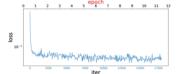
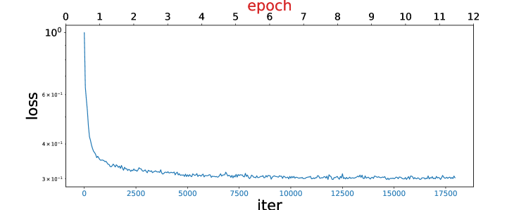
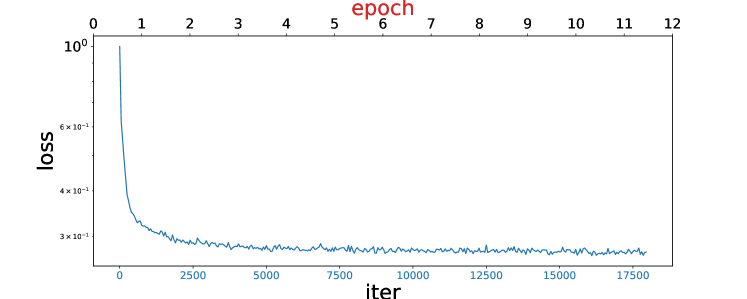
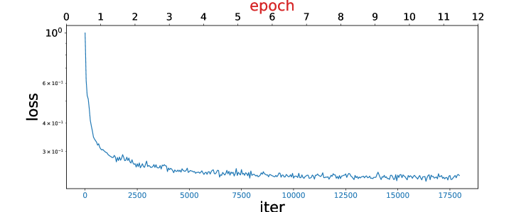
Figure 4: Loss drop in task Inpainting, dataset CelebA. These corresponds to four different initializations used in our experiments, namely Fourier, Kaiming Uniform, Kaiming Normal and Orthogonal.

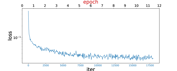
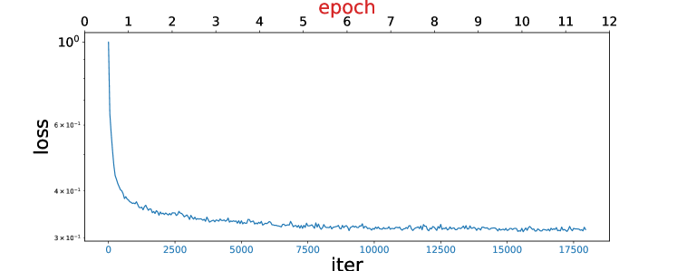
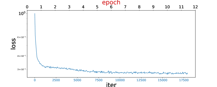
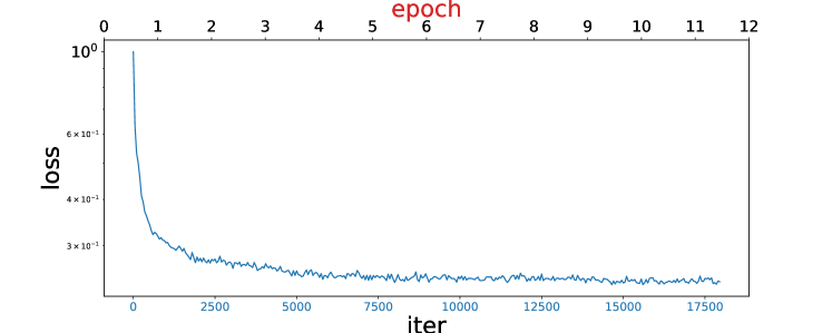
Figure 5: Loss drop in task Deblurring, dataset CelebA. These corresponds to four different initializations used in our experiments, namely Fourier, Kaiming Uniform, Kaiming Normal and Orthogonal.

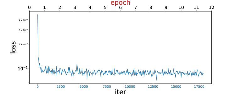
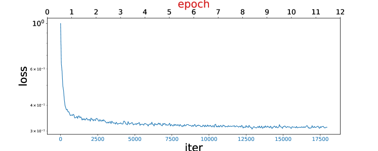
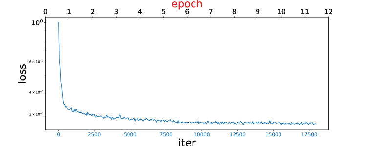
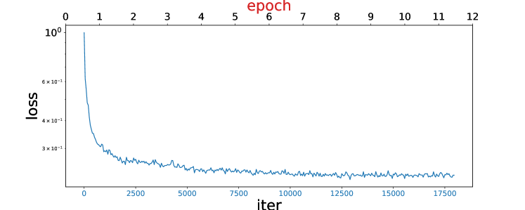
Figure 6: Loss drop in task Denoising, dataset CelebA. These corresponds to four different initializations used in our experiments, namely Fourier, Kaiming Uniform, Kaiming Normal and Orthogonal.

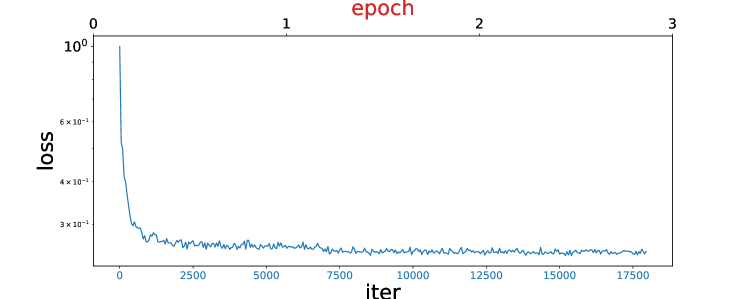
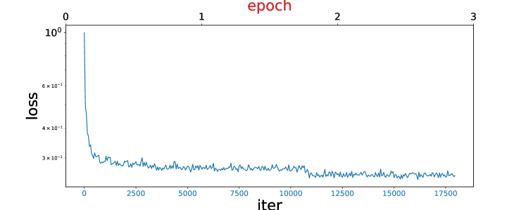
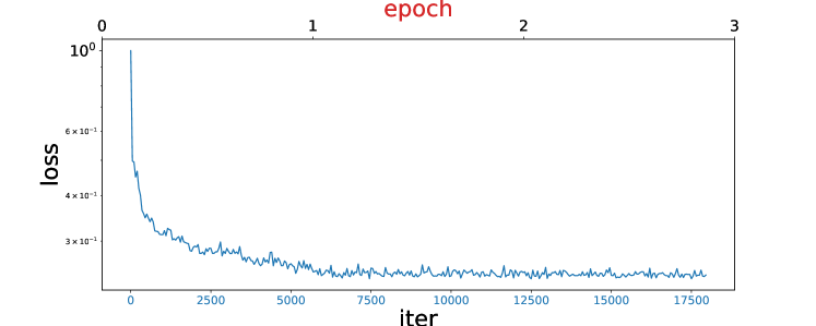
Figure 7: Loss drop in task watermark removal, dataset CelebA. These corresponds to four different initializations used in our experiments, namely Fourier, Kaiming Uniform, Kaiming Normal and Orthogonal.

References

- [1] Dulari Bhatt, Chirag Patel, Hardik Talsania, Jigar Patel, Rasmika Vaghela, Sharnil Pandya, Kirit Modi, and Hemant Ghayvat. Cnn variants for computer vision: History, architecture, application, challenges and future scope. Electronics, 10(20):2470, 2021.
- [2] Yann LeCun, Léon Bottou, Yoshua Bengio, and Patrick Haffner. Gradient-based learning applied to document recognition. Proceedings of the IEEE, 86(11):2278–2324, 1998.
- [3] Alex Krizhevsky, Ilya Sutskever, and Geoffrey E Hinton. Imagenet classification with deep convolutional neural networks. Communications of the ACM, 60(6):84–90, 2017.
- [4] Kaiming He, Georgia Gkioxari, Piotr Dollar, and Ross Girshick. Mask r-cnn. In Proceedings of the IEEE International Conference on Computer Vision (ICCV), Oct 2017.
- [5] Yinhao Ren, Zhe Zhu, Yingzhou Li, Dehan Kong, Rui Hou, Lars J Grimm, Jeffery R Marks, and Joseph Y Lo. Mask embedding for realistic high-resolution medical image synthesis. In International Conference on Medical Image Computing and Computer-Assisted Intervention, pages 422–430. Springer, 2019.
- [6] Olaf Ronneberger, Philipp Fischer, and Thomas Brox. U-net: Convolutional networks for biomedical image segmentation. In International Conference on Medical image computing and computer-assisted intervention, pages 234–241. Springer, 2015.
- [7] Rajiv Saxena and Kulbir Singh. Fractional fourier transform: A novel tool for signal processing. Journal of the Indian Institute of Science, 85(1):11, 2005.
- [8] Lawrence R Rabiner and Bernard Gold. Theory and application of digital signal processing. Englewood Cliffs: Prentice-Hall, 1975.
- [9] Hadhrami Ab Ghani, Mohamad Razwan Abdul Malek, Muhammad Fadzli Kamarul Azmi, Muhammad Jefri Muril, and Azizul Azizan. A review on sparse fast fourier transform applications in image processing. International Journal of Electrical & Computer Engineering (2088-8708), 10(2), 2020.
- [10] Isa Servan Uzun, Abbes Amira, and Ahmed Bouridane. Fpga implementations of fast fourier transforms for real-time signal and image processing. IEE Proceedings-Vision, Image and Signal Processing, 152(3):283–296, 2005.
- [11] Li Xu, Shicheng Zheng, and Jiaya Jia. Unnatural l0 sparse representation for natural image deblurring. In Proceedings of the IEEE conference on computer vision and pattern recognition, pages 1107–1114, 2013.
- [12] James W Cooley, Peter AW Lewis, and Peter D Welch. Historical notes on the fast fourier transform. Proceedings of the IEEE, 55(10):1675–1677, 1967.
- [13] James W Cooley, Peter AW Lewis, and Peter D Welch. The fast fourier transform and its applications. IEEE Transactions on Education, 12(1):27–34, 1969.
- [14] Emmanuel Candes, Laurent Demanet, and Lexing Ying. A fast butterfly algorithm for the computation of fourier integral operators. Multiscale Modeling & Simulation, 7(4):1727–1750, 2009.
- [15] Yingzhou Li and Haizhao Yang. Interpolative butterfly factorization. SIAM Journal on Scientific Computing, 39(2):A503–A531, 2017.
- [16] Yingzhou Li, Haizhao Yang, Eileen R. Martin, Kenneth L. Ho, and Lexing Ying. Butterfly factorization. Multiscale Modeling & Simulation, 13(2):714–732, 2015.
- [17] Yingzhou Li, Haizhao Yang, and Lexing Ying. A multiscale butterfly algorithm for multidimensional fourier integral operators. Multiscale Modeling & Simulation, 13(2):614–631, 2015.
- [18] Yingzhou Li, Haizhao Yang, and Lexing Ying. Multidimensional butterfly factorization. Applied and Computational Harmonic Analysis, 44(3):737–758, 2018.
- [19] Lexing Ying. Sparse fourier transform via butterfly algorithm. SIAM Journal on Scientific Computing, 31(3):1678–1694, 2009.
- [20] John Denker, W Gardner, Hans Graf, Donnie Henderson, R Howard, W Hubbard, Lawrence D Jackel, Henry Baird, and Isabelle Guyon. Neural network recognizer for hand-written zip code digits. Advances in neural information processing systems, 1, 1988.
- [21] Yutong Xie, Jianpeng Zhang, Chunhua Shen, and Yong Xia. Cotr: Efficiently bridging cnn and transformer for 3d medical image segmentation. In International conference on medical image computing and computer-assisted intervention, pages 171–180. Springer, 2021.
- [22] Kai Zhang, Wangmeng Zuo, Shuhang Gu, and Lei Zhang. Learning deep cnn denoiser prior for image restoration. In Proceedings of the IEEE conference on computer vision and pattern recognition, pages 3929–3938, 2017.
- [23] Yanting Pei, Yaping Huang, Qi Zou, Hao Zang, Xingyuan Zhang, and Song Wang. Effects of image degradations to cnn-based image classification. arXiv preprint arXiv:1810.05552, 2018.
- [24] Felipe Cucker and Ding Xuan Zhou. Learning theory: an approximation theory viewpoint, volume 24. Cambridge University Press, 2007.
- [25] Allan Pinkus. Approximation theory of the mlp model in neural networks. Acta numerica, 8:143–195, 1999.
- [26] Yingzhou Li, Xiuyuan Cheng, and Jianfeng Lu. Butterfly-net: Optimal function representation based on convolutional neural networks. arXiv preprint arXiv:1805.07451, 2018.
- [27] Harry Pratt, Bryan Williams, Frans Coenen, and Yalin Zheng. Fcnn: Fourier convolutional neural networks. In Joint European Conference on Machine Learning and Knowledge Discovery in Databases, pages 786–798. Springer, 2017.
- [28] Zongyi Li, Nikola Kovachki, Kamyar Azizzadenesheli, Burigede Liu, Kaushik Bhattacharya, Andrew Stuart, and Anima Anandkumar. Fourier neural operator for parametric partial differential equations. arXiv preprint arXiv:2010.08895, 2020.
- [29] Beidi Chen, Tri Dao, Kaizhao Liang, Jiaming Yang, Zhao Song, Atri Rudra, and Christopher Re. Pixelated butterfly: Simple and efficient sparse training for neural network models. arXiv preprint arXiv:2112.00029, 2021.
- [30] Tri Dao, Albert Gu, Matthew Eichhorn, Atri Rudra, and Christopher Ré. Learning fast algorithms for linear transforms using butterfly factorizations. In International conference on machine learning, pages 1517–1527. PMLR, 2019.
- [31] Zhongshu Xu, Yingzhou Li, and Xiuyuan Cheng. Butterfly-net2: Simplified butterfly-net and fourier transform initialization. In Mathematical and Scientific Machine Learning, pages 431–450. PMLR, 2020.
- [32] Davis Gilton, Greg Ongie, and Rebecca Willett. Neumann networks for linear inverse problems in imaging. IEEE Transactions on Computational Imaging, 6:328–343, 2019.