Adaptive Scenario Subset Selection for Worst-Case Optimization
and its Application to Well Placement Optimization

Abstract

In this study, we consider simulation-based worst-case optimization problems with continuous design variables and a finite scenario set. To reduce the number of simulations required and increase the number of restarts for better local optimum solutions, we propose a new approach referred to as adaptive scenario subset selection (AS3). The proposed approach subsamples a scenario subset as a support to construct the worst-case function in a given neighborhood, and we introduce such a scenario subset. Moreover, we develop a new optimization algorithm by combining AS3 and the covariance matrix adaptation evolution strategy (CMA-ES), denoted AS3-CMA-ES. At each algorithmic iteration, a subset of support scenarios is selected, and CMA-ES attempts to optimize the worst-case objective computed only through a subset of the scenarios. The proposed algorithm reduces the number of simulations required by executing simulations on only a scenario subset, rather than on all scenarios. In numerical experiments, we verified that AS3-CMA-ES is more efficient in terms of the number of simulations than the brute-force approach and a surrogate-assisted approach lq-CMA-ES when the ratio of the number of support scenarios to the total number of scenarios is relatively small. In addition, the usefulness of AS3-CMA-ES was evaluated for well placement optimization for carbon dioxide capture and storage (CCS). In comparison with the brute-force approach and lq-CMA-ES, AS3-CMA-ES was able to find better solutions because of more frequent restarts.

1 Introduction

1.1 Background

Simulation-based optimization is becoming popular in various industrial fields as computational performance increases. Such optimization evaluates the objective function value of a solution candidate by a computationally expensive numerical simulation. Evolutionary approaches have been successfully applied to simulation-based optimization in a variety of engineering fields. Many examples of such applications have been reported in the relevant literature [1, 2, 3, 4, 5, 6, 7, 8, 9, 10, 11, 12, 13, 14]. Evolutionary approaches are preferred for several reasons. First, because they do not require gradient information, they can be easily applied to simulation-based optimization, where the gradient is often unavailable. Second, they empirically exhibit better performance on problems with multiple local optima than approaches using local information, such as the gradient of the objective [15]. Third, they can be easily accelerated by running simulations for multiple solution candidates in parallel. Hence, although evolutionary approaches tend to require a relatively high number of function evaluations, the execution time of the optimization process can be easily reduced [16].

The objective of simulation-based optimization is typically to locate a solution whose performance is satisfactory in the real-world environment. For this purpose, we design a numerical model to simulate the objective function. However, there is often a discrepancy between the numerical model and the real-world environment. The uncertainty in the real-world environment owing to limited information is a key reason for this divergence. Because of the uncertainty, there may be multiple numerical models that are consistent with the information of the real-world environment. A naive approach often applied in engineering optimization practice is to choose one such model, denoted as $f_{\mathrm{sim}}$, optimize (here, we assume minimization without loss of generality) $f_{\mathrm{sim}}$ and obtain a solution $x^{*}$, and evaluate it in the real-world environment, denoted by $f_{\mathrm{real}}$. However, because of the discrepancy between $f_{\mathrm{sim}}$ and $f_{\mathrm{real}}$, the solution $x^{*}$ obtained in the simulation is not guaranteed to exhibit satisfactory performance in the real-world environment. That is, we may obtain $f_{\mathrm{real}}(x^{*})\gg f_{\mathrm{sim}}(x^{*})$.

A possible approach is to formulate the problem as a min–max optimization, where the objective is to locate the optimal solution to the worst-case objective function among all possible numerical models. Assume that we have $m$ different numerical models indexed by $s\in S=\{1,\dots,m\}$. Then, the min–max optimization problem is formulated as

$$\min_{x\in\mathbb{X}}\max_{s\in S}f(x,s)\enspace,$$ (1)

where $x\in\mathbb{X}\subseteq\mathbb{R}^{n}$ represents the design variable, $s\in S$ is the scenario index, and $f:\mathbb{X}\times S\to\mathbb{R}$ is the objective function. It is recognized as the minimization of the worst-case objective function $F(x)=\max_{s\in S}f(x,s)$, which can be explicitly evaluated because $S$ is a finite set. Because $F$ is tractable, a simple evolutionary approach can be applied to minimize $F$. However, each $F$ call costs (requires) $m$ simulations (i.e., $f$-calls), with a corresponding increase in the computation time with greater $m$.

The aim of this study is to develop an efficient approach to address min–max optimization (1). We assume the following. (I) The scenario set $S$ is a finite set; therefore, we can evaluate the worst-case objective $F$ analytically. (II) The $f$-call is computationally expensive, and the number of $f$-calls is the bottleneck of the optimization process. (III) $f$ is black-box and its gradient information is unavailable. A derivative-free approach such as an evolutionary approach is required. (IV) $f$ and $F$ are non-convex, and there are multiple local optima. To obtain a satisfactory local optimal solution, a restart strategy is required. However, because each $F$-call requires $m$ $f$-calls and each $f$-call is computationally demanding, we may be able to perform only a few restarts within a given time budget if we naively optimize $F$. Based on the observation in the following motivational application, we further assume the following characteristics. (V) For any $s\in S$, there exists $x\in\mathbb{X}$ such that $F(x)=f(x,s)$. That is, without having all $s$, we cannot construct the true worst-case objective function. However, (VI) if we limit our attention to the neighborhood of a local optimal solution, $F$ can be constructed using a subset $A\subset S$ with a relatively small cardinality $\lvert A\rvert/\lvert S\rvert$. Note also that characteristics (V) and (VI) are not requirements for the proposed approach to work properly and they cannot be confirmed prior to the start of optimization. Although characteristics (V) and (VI) are observations on a specific application, we conjecture that these characteristics appear in other simulation-based optimization problems. By utilizing characteristics (V) and (VI), we expect to reduce the number of $f$-calls to optimize $F$, resulting in more restarts and obtaining a better local optimum.

1.2 Motivational Application

Our motivational application considers well placement optimization for carbon dioxide capture and storage (CCS) projects [17]. CCS is a promising technique developed to reduce $\mathrm{CO_{2}}$ emissions by capturing $\mathrm{CO_{2}}$ in exhaust gases and injecting the captured $\mathrm{CO_{2}}$ into a reservoir deep underground through wells. The objective of well placement optimization in CCS is to determine the well placement that provides as much benefit (e.g., total $\mathrm{CO_{2}}$ injection volume) as possible with the least cost (e.g., drilling expenses) and risk (e.g., pressure build-up in the reservoir). Simulation-based optimization is among the possible approaches for these projects. The well placement is optimized through simulations that take a design variable, which encodes well coordinates, injection or production rate schedules, and well types (vertical / horizontal / multilateral), along with similar information, as an input and returns the abovementioned criteria. To perform numerical simulations, experts design numerical models that describe geological conditions, such as the distribution of physical properties or boundary conditions resulting from geological surveys. However, in general, numerical models contain various uncertainties because geological surveys and investigations are limited. For instance, exploration wells are drilled to sample and investigate the physical properties of sites; however, they are insufficient to cover a vast geological formation, and the property distribution between exploration wells is highly uncertain. To deal with such uncertainties, multiple numerical models have been created using the same limited information. In previous studies, different criteria such as the average, the worst case, and the value at risk have been applied to obtain robust solutions under multiple numerical models [9, 18, 19, 20, 21]. Among the different formulations, the min–max optimization (1) is suitable to guarantee the commerciality or feasibility of the project in the worst scenario.

Here, we summarize the important characteristics of this application. First, simulations executed to evaluate $f(x,s)$ are computationally demanding, as they require multicomponent and multiphase fluid simulators. For example, previous studies [16, 22] have reported one simulation taking several hours to complete. Therefore, the number of $f$-calls is limited for the optimization. Second, the scenario set $S$ is a finite set. This uncertainty is represented by numerical models created by experts. Although we cannot guarantee that the real-world environment is included in $S$, we expect the solution to the worst-case objective function under different numerical models created by experts to become reliable as we increase the number $m$ of scenarios. Third, $f(x,s)$ is a black box, and no gradient information is available. Fourth, $f$ and $F(x)$ are non-convex. Finally, we observe characteristics (V) and (VI) in Figure 8, as discussed in Section 5.

1.3 Related work

Studies on derivative-free worst-case optimization under finite scenarios may be categorized into two classes. One focuses on the smoothness of the worst-case objective function $F$. It becomes naturally non-smooth owing to its construction. For some derivative-free optimization approaches, the smoothness of the objective function is important for its success. Some studies have been conducted along these lines; for example, [23, 24, 25], in which $F$ was approximated by a smooth function, and a derivative-free optimization method was applied to minimize the approximate function so as not to fail to locate a local optimal solution owing to the non-smoothness of $F$. The other research direction that has been explored involves reducing the computation cost. The evaluation of the worst-case objective value $F(x)$ for each $x$ requires $m$ simulations to compute $f(x,s)$ for $s\in S$, and each $f$-call is computationally demanding. Therefore, the computation cost is often a primary bottleneck in practice. Reducing the computation cost allows more restarts to be performed, thereby increasing the chance of obtaining better solutions if the objective is non-convex. These two research directions are orthogonal, and these ideas may be combined. Nevertheless, in this study, we focus on the latter topic.

The following two approaches have been investigated to reduce the computation cost of the optimization.

The first approach is to subsample scenarios from scenario set $S$ before optimization by using domain knowledge. In other words, the computation cost can be reduced by preliminarily decreasing the number of scenarios used for the optimization. This approach has been applied in the optimization of the designs or operations of oil fields. Prior to optimization, some criteria, such as the potential oil volume per scenario evaluated by numerical simulation, are prepared. Then, scenarios are subsampled based on the prepared criteria, and optimization is performed on the subsampled scenarios [26, 27, 28, 29, 30, 31, 32, 33]. This approach assumes that the worst-case objective function on the scenario set $S$ can be approximated on a subset $A$. However, this assumption is not generally satisfied. The approaches of this type are domain-specific and cannot be applied to other problems directly.

Surrogate-assisted approaches are the other primary alternative. They can reduce the number of $f$-calls by approximating $F(x)$ with a surrogate model trained during the optimization [34, 35, 36, 37]. Because the quality of the surrogate model determines the effectiveness of these approaches, various methods such as a linear-quadratic model [37] or Kriging [36] have been studied. These methods are effective when the objective function is smooth; however, the worst-case objective function $F$ becomes naturally non-smooth. Therefore, it may be difficult to select a proper surrogate model to approximate $F$.

1.4 Contributions

In this study, we develop and evaluate a novel approach for the min–max optimization problem (1) with finite scenarios satisfying Assumptions (I)–(VI) described above.The contributions of this study are summarized as follows.

1. We define the notion of support scenarios $S_{\mathrm{support}}(H)$ in a subset $H$ of the search space $\mathbb{X}$. This notion is used to describe the subset of scenarios that are sufficient to compute the worst-case objective function value for a solution candidate generated from the current search distribution with high probability. Assumptions (V) and (VI) above mean that the number of support scenarios is equivalent to the number of all scenarios at the beginning of the search, where the search distribution is widely spread, whereas it is significantly smaller if the search distribution is concentrated around a local optimal solution. We utilize this notion to develop the proposed approach and develop test problems.

2. We propose an adaptive scenario subset selection (AS3) mechanism. AS3 attempts to reduce the number of $f$-calls required to compute the worst-case objective function values during the optimization by approximately sampling the support scenarios corresponding to the search distribution at each iteration. In contrast to general-purpose surrogate-assisted approaches, AS3 is specialized for worst-case optimization. Further, compared to domain-specific approaches that subsample scenarios prior to optimization based on some prior knowledge, AS3 does not require such prior knowledge. AS3 mechanism was integrated into the CMA-ES. The resulting approach is called AS3-CMA-ES. Numerical experiments showed that AS3 mechanism follows the change in the support scenarios in the area $H_{\gamma}^{t}$, where the solution candidates are generated with probability $\gamma$ at iteration $t$. That is, AS3 successfully reduced the number of $f$-calls on problems where Assumption (VI) holds.

3. We compared AS3-CMA-ES with the brute-force approach optimizing $F$ directly using the CMA-ES and a surrogate-assisted approach, lq-CMA-ES [37], on test problems. We confirmed that AS3-CMA-ES outperforms the brute-force approach in terms of the number of $f$-calls in most cases. Moreover, AS3-CMA-ES was more efficient than lq-CMA-ES for problems satisfying Assumption (VI), where lq-CMA-ES is more efficient if the number of support scenarios around the local optimal solution is close to the number of scenarios.

4. The effectiveness of AS3-CMA-ES was evaluated in a real-world application (well placement optimization for CCS) and comparison with lq-CMA-ES and the brute-force approach. The experimental results show that AS3-CMA-ES achieves a better solution within a given $f$-call budget than the compared approaches because of more restarts owing to its faster convergence, leading to a better local optimal solution for multimodal problems.

The remainder of this paper is organized as follows. The baseline approach—the brute-force approach optimizing $F$ using the CMA-ES—is introduced in Section 2. The proposed approach is explained in Section 3. The numerical experiments performed to demonstrate the efficiency of the proposed algorithm are outlined in Section 4. The comparisons carried out with the baseline approaches are also discussed. The utilization of the proposed algorithm for well placement optimization is presented in Section 5. Concluding remarks are presented in Section 6. Some experimental results are provided in the appendices to further elucidate the usefulness of the proposed approach.

2 CMA-ES: Covariance Matrix Adaptation Evolution Strategy (baseline approach)

Our baseline approach optimizes $x\in\mathbb{X}$ on the worst-case objective function $F$. For a solution candidate $x\in\mathbb{X}$, $F(x)$ can be evaluated by evaluating $m$ $f$-calls, i.e., $f(x,1),\dots,f(x,m)$, and by taking their maximum $\max_{s\in S}f(x,s)$.

We employ the covariance matrix adaptation evolution strategy (CMA-ES) [39, 40, 41] with a restart strategy as the baseline approach. The CMA-ES is recognized as a state-of-the-art derivative-free approach for black-box continuous optimization of non-convex functions [15, 42]. The CMA-ES is a quasi-parameter-free approach. That is, the users of this approach need not tune its hyperparameters on their own tasks, but rather can use it out-of-the-box. This property and its superior performance have attracted practitioners, and hence, the CMA-ES has been widely applied to real-world applications [1, 2, 3, 4, 5, 6, 7, 8, 9, 10, 11, 12, 13, 14].

Algorithm 1 The baseline approach

1:$m^{0}\in\mathbb{R}^{n}$, $\Sigma^{0}\in\mathbb{R}^{n\times n}$

2:$\lambda_{x}\leftarrow\lfloor 4+3\log(n)\rfloor$

3:for $t=0,\dots,T-1$ do

4:    for $k=1,\dots,\lambda_{x}$ do

5:         Sample $x^{t}_{k}\sim\mathcal{N}(m^{t},\Sigma^{t})$.

6:         Evaluate $f^{t}_{k,s}=f(x^{t}_{k},s)$ for all $s\in S$.

7:         Set $F^{t}_{k}=\max_{s\in S}f^{t}_{k,s}$.

8:    end for

9:    Perform CMA-ES update using $\{(x^{t}_{k},F^{t}_{k})\}_{k=1}^{\lambda_{x}}$

10:    if converged then

11:         Reset $m^{t+1}$ and $\Sigma^{t+1}$ (and possibly change $\lambda_{x}$)

12:    end if

13:end for

Our baseline approach—the CMA-ES, optimizing the worst-case objective $F$—is outlined in Algorithm 1. The population size $\lambda_{x}$, i.e., the number of solution candidates generated at each iteration, is set based on the search space dimension $n$. At each iteration, the CMA-ES generates $\lambda_{x}$ solution candidates, $x_{k}^{t}$ ($k=1,\dots,\lambda_{x}$) from the multivariate normal distribution $\mathcal{N}(m^{t},\Sigma^{t})$ with mean $m^{t}$ and $\Sigma^{t}$. Each solution candidate is evaluated on $f(\cdot,s)$ for all scenarios $s\in S$. Then, the worst-case objective function value $F(x_{k}^{t})$ for each $x_{k}^{t}$ is computed by $\max_{s\in S}f(x_{k}^{t},s)$ and assigned to $F_{k}^{t}$. Using the pairs $\{(x_{k}^{t},F_{k}^{t})\}$ of the solution candidates and their worst-case objective function values, the CMA-ES updates the distribution parameters $m$ and $\Sigma$, and other dynamic parameters used for their updates. These updates are known to follow the natural gradient of the expected objective function value [46]. These steps are repeated until the distribution is regarded as converged. Once the distribution converges, the current mean vector is registered as a candidate local optimal solution. Then, the mean vector and the covariance matrix are reset for restart.

Of note, this brute-force approach to optimizing $F$ involves an important limitation. Because $F$ is assumed to be non-convex and possibly multimodal, it is essential to perform as many restarts as possible. However, to evaluate the worst-case objective function value $F(x)$ for each solution candidate $x$, $m$ $f$-calls are required. That is, as the number $m$ of the scenarios increases, this approach can perform fewer restarts, possibly leading to a poorer local optimal solution.

3 Adaptive Scenario Subset Selection (AS3) Mechanism

We propose a new approach, namely adaptive scenario subset selection (AS3), to reduce the number of $f$-calls for each restart and to enable more restarts to be performed for a better local optimal solution. This section presents the design principles and details of AS3.

3.1 Design Principles

Our idea is to save $f$-calls when computing the worst-case objective function value $F$ at each iteration of Algorithm 1 without changing its behavior. For this purpose, we wish to subsample a scenario set $A^{t}\subseteq S$ at each iteration $t$ such that $F(x_{k}^{t})=F(x_{k}^{t};A^{t})$ for all $k=1,\dots,\lambda_{x}$, where $F(x;A^{t})$ is the worst-case objective function under the scenario subset $A^{t}$ and is defined as $F(x;A^{t})=\max_{s\in A^{t}}f(x,s)$. If we can select a subset $A^{t}$ with $\lvert A^{t}\rvert/\lvert S\rvert<1$, we can save $\lvert S\rvert-\lvert A_{t}\rvert$ $f$-calls for the evaluation of the worst-case objective function value $F(x_{k}^{t})$ of each solution candidate $x_{k}^{t}$ without changing the algorithmic behavior. However, $A^{t}$ cannot be known without evaluating $f(x_{k}^{t},s)$ for all $s\in S$ as $f$ is a black box. Therefore, we estimate $A^{t}$ during the optimization.

To estimate $A^{t}$, we utilize information about a neighborhood in which solution candidates are expected to be generated at each iteration. Let $x$ be $\mathcal{N}(m,\Sigma)$-distributed. Then, it is easy to see that $(x-m)^{\mathrm{T}}\Sigma^{-1}(x-m)$ is $\chi^{2}_{n}$-distributed with the degrees of freedom of $n$. In other words, $(x-m)^{\mathrm{T}}\Sigma^{-1}(x-m)\leqslant P_{\chi_{n}^{2}}^{-1}(\gamma)$ with probability $\gamma\in[0,1]$, where $P_{\chi_{n}^{2}}$ is the cumulative density function of a $\chi^{2}$ distribution with $n$ degrees of freedom. Because the CMA-ES samples solution candidates from $\mathcal{N}(m^{t},\Sigma^{t})$, each solution candidate falls into

$$H^{t}_{\gamma}=\left\{x\in\mathbb{R}^{n}:(x-m^{t})^{\mathrm{T}}(\Sigma^{t})^{-1}(x-m^{t})\leqslant P_{\chi_{n}^{2}}^{-1}(\gamma)\right\},$$ (2)

with probability $\gamma$. Therefore, if we can select $A^{t}\subseteq S$ such that $F(x)=F(x;A^{t})$ for all $x\in H_{\gamma}^{t}$, and we set $\gamma$ close to $1$, we need to evaluate $f(x,s)$ only for all $s\in A^{t}$ to compute $F(x)$, i.e., $\lvert A^{t}\rvert$ $f$-calls are required. Hence, we can omit $\lvert S\setminus A^{t}\rvert$ $f$-calls for each solution candidate while mimicking the behavior of the baseline approach (Algorithm 1), which evaluates $f(x,s)$ for all $s\in S$ to compute $F(x)$, requiring $\lvert S\rvert$ $f$-calls.

To formalize our idea, we define the notion of support scenarios.

Definition 3.1 (Support Scenario).

A scenario $s\in S$ such that $F(x)=f(x,s)$ at $x\in\mathbb{X}$ is called a support scenario of $x$. A scenario $s\in S$ is called a support scenario in neighborhood $H\subseteq\mathbb{X}$ if there exists $x\in H$ such that $F(x)=f(x,s)$. The set of support scenarios in $H$ is denoted by $S_{\mathrm{support}}(H)\subseteq S$. If $s\in S$ is a support scenario in all neighborhoods $H$ of $x^{*}\in\mathbb{X}$, it is called a support scenario around $x^{*}$. The set of support scenarios around $x^{*}$ is denoted by $S_{\mathrm{support}}(x^{*})=\bigcap_{x^{*}}S_{\mathrm{support}}(H)\subseteq S$, where $\bigcap_{x^{*}}$ is the intersection of all neighborhoods of $x^{*}$.

Our idea is to select $A^{t}=S_{\mathrm{support}}(H_{\gamma}^{t})$ at each iteration and use $F(x;S_{\mathrm{support}}(H_{\gamma}^{t}))$ as a surrogate of $F$. Then, the worst-case objective function value of each solution candidate is correctly computed with probability $\gamma$, whereas $\lvert S\rvert-\lvert S_{\mathrm{support}}(H_{\gamma}^{t})\rvert$ $f$-calls are omitted. The smaller $\lvert S_{\mathrm{support}}(H^{t}_{\gamma})\rvert/\lvert S\rvert$, the more efficient the subsampling becomes.

Although the worst-case objective function values of $(1-\gamma)\cdot\lambda_{x}$ solution candidates are underestimated ($F(x)\geqslant F(x;A^{t})$), the effect of such solution candidates on the algorithmic behavior is expected to be small. This is because the CMA-ES is a ranking-based approach (hence, the magnitude of the difference $F(x)-F(x;A^{t})$ itself does not matter), and the ranking change due to the underestimation of $F(x)$ is restricted.

Remark 3.2.

To estimate the effect of the underestimation of $F(x)$ by $G(x)=F(x;S_{\mathrm{support}}(H_{\gamma}^{t}))$, we consider the population version of Kendall’s rank correlation $\tau$, defined as

$$\tau=\Pr[(F(X)-F(Y))(G(X)-G(Y))>0]-\Pr[(F(X)-F(Y))(G(X)-G(Y))<0]\enspace,$$ (3)

where $X$ and $Y$ are solution candidates and are independently $\mathcal{N}(m^{t},\Sigma^{t})$-distributed. For technical simplicity, we assume that all the level sets of $F$ and $G$ have zero Lebesgue measure (roughly speaking, there is no constant area). Then, because $\Pr[F(X)=F(Y)]=\Pr[G(X)=G(Y)]=0$, we have

$$\Pr[(F(X)-F(Y))(G(X)-G(Y))>0]=\Pr[(F(X)-F(Y))(G(X)-G(Y))\geqslant 0]\\ =1-\Pr[(F(X)-F(Y))(G(X)-G(Y))\leqslant 0]=1-\Pr[(F(X)-F(Y))(G(X)-G(Y))<0].$$ (4)

Therefore, $\tau=2\Pr[(F(X)-F(Y))(G(X)-G(Y))\geqslant 0]-1$. If $X$ and $Y$ are both in $H_{\gamma}^{t}$, which occurs with probability $\Pr[X,Y\in H_{\gamma}^{t}]=\gamma^{2}$, we have $F(X)=G(X)$ and $F(Y)=G(Y)$. Then, we have

$$\Pr[(F(X)-F(Y))(G(X)-G(Y))\geqslant 0\mid X,Y\in H_{\gamma}^{t}]=\Pr[(F(X)-F(Y))^{2}\geqslant 0\mid X,Y\in H_{\gamma}^{t}]=1\enspace.$$ (5)

Hence,

$$\begin{split}&\Pr[(F(X)-F(Y))(G(X)-G(Y))\geqslant 0]\\ &=\Pr[(F(X)-F(Y))(G(X)-G(Y))\geqslant 0\mid X,Y\in H_{\gamma}^{t}]\Pr[X,Y\in H_{\gamma}^{t}]\\ &\quad+\Pr[(F(X)-F(Y))(G(X)-G(Y))\geqslant 0\mid\neg(X,Y\in H_{\gamma}^{t})]\Pr[\neg(X,Y\in H_{\gamma}^{t})]\\ &\geqslant\Pr[(F(X)-F(Y))(G(X)-G(Y))\geqslant 0\mid X,Y\in H_{\gamma}^{t}]\Pr[X,Y\in H_{\gamma}^{t}]=\gamma^{2}\enspace.\end{split}$$ (6)

Finally, we obtain $\tau\geqslant 2\gamma^{2}-1$. That is, the rank correlation between $F(x)$ and $F(x;S_{\mathrm{support}}(H_{\gamma}^{t}))$ under $x\sim\mathcal{N}(m^{t},\Sigma^{t})$ is lower-bounded by $2\gamma^{2}-1$, which can be made arbitrarily close to one by setting $\gamma$ close to $1$. Although we do not analyze the relation between $\tau$ and the algorithmic behavior theoretically here, $\tau$ is used to measure the goodness of surrogate models in practice [37, 47]. Hence, we expect that a sufficiently high $\tau$ value will lead to sufficiently close behavior.

To estimate $S_{\mathrm{support}}(H_{\gamma}^{t})$ during optimization, we introduce $p^{t}=(p_{1}^{t},\cdots,p_{m}^{t})\in[0,1]^{m}$, where $p_{s}^{t}$ indicates the certainty of the algorithm whether $s\in S$ is in $S_{\mathrm{support}}(H_{\gamma}^{t})$. Ideally, we want $p_{s}^{t}=\mathbb{I}\{s\in S_{\mathrm{support}}(H_{\gamma}^{t})\}$, where it is $1$ if $s\in S_{\mathrm{support}}(H^{t}_{\gamma})$ and $0$ otherwise. Then, by using $p_{s}^{t}$ as the probability of sampling a scenario $s\in S$ to construct a subset $A^{t}$, we obtain $A^{t}=S_{\mathrm{support}}(H_{\gamma}^{t})$. Because the search distribution of the CMA-ES changes gradually over the series of iterations, $H_{\gamma}^{t}$ also does so. Then, we expect that $S_{\mathrm{support}}(H_{\gamma}^{t})$ also changes gradually with iteration. Therefore, we maintain $p^{t}$ over iterations. In the next section, we describe a heuristic approach to maintain $p^{t}$.

3.2 Parameter Update

At each iteration, we sample $A^{t}\subseteq S$ by using a binomial distribution with probability $p_{s}^{t}$ of sampling scenario $s$ and evaluate the solution candidates $x_{1}^{t},\dots,x_{\lambda_{x}}^{t}$ on $f(x,s)$ for $s\in A^{t}$. Therefore, we can observe whether $F(x_{k}^{t};A^{t})=f(x_{k}^{t};s)$ for each $s\in A^{t}$. If $S_{\mathrm{support}}(H_{\gamma}^{t})\subseteq A_{t}$, $F(x_{k}^{t};A^{t})=f(x_{k}^{t};s)$ for some $x_{k}^{t}\in H_{\gamma}^{t}$ indicates that $s\in S_{\mathrm{support}}(H_{\gamma}^{t})$. If $S_{\mathrm{support}}(H_{\gamma}^{t})\not\subseteq A_{t}$, $F(x_{k}^{t};A^{t})=f(x_{k}^{t};s)$ for some $x_{k}^{t}\in H_{\gamma}^{t}$ does not necessarily mean $s\in S_{\mathrm{support}}(H_{\gamma}^{t})$. Because the algorithm cannot distinguish the above two situations, we increase $p_{s}^{t}$ for such scenarios. However, we know that $F(x_{k}^{t};A^{t})>f(x_{k}^{t};s)$ for all $x_{k}^{t}\in H_{\gamma}^{t}$ does not provide information on whether $s\in S_{\mathrm{support}}(H_{\gamma}^{t})$ because there may exist $x\in H_{\gamma}^{t}\setminus\{x_{k}^{t}\}_{k=1}^{\lambda_{x}}$ such that $F(x)=f(x,s)$. However, the probability of such an event is $(1-\Pr[F(x)=f(x,s)\wedge x\in H_{\gamma}^{t}\mid x\sim\mathcal{N}(m^{t},\Sigma^{t})])^{\lambda_{x}}$, which is sufficiently small as we set $\lambda_{x}$ to a large value. Therefore, we decrease $p_{s}^{t}$ for scenarios with $F(x_{k}^{t};A^{t})>f(x_{k}^{t};s)$ for all $x_{k}^{t}\in H_{\gamma}^{t}$. For $s\not\in A^{t}$, we have no information on whether $s\in S_{\mathrm{support}}(H_{\gamma}^{t})$. Hence, we keep $p_{s}^{t}$.

To realize this idea, we update $p^{t}_{s}$ as $p^{t+1}_{s}=p^{t}_{s}+\Delta^{t}_{s}$, where

$$\Delta_{s}^{t}=\mathbb{I}\{s\in A^{t}\}\cdot\left(c_{p}\cdot\sum_{i=1}^{\lambda_{x}}\mathbb{I}\{F(x^{t}_{i};A^{t})=f(x^{t}_{i},s)\wedge x^{t}_{i}\in H^{t}_{\gamma}\}-c_{n}\cdot\prod_{i=1}^{\lambda_{x}}(1-\mathbb{I}\{F(x^{t}_{i};A^{t})=f(x^{t}_{i},s)\wedge x^{t}_{i}\in H^{t}_{\gamma}\})\right)\enspace.$$ (7)

Here, $c_{p}$ is the learning rate for the increase in $p_{s}^{t}$, and $c_{n}$ is the learning rate for the decrease in $p_{s}^{t}$. The first term is $c_{p}$ times the number of solution candidates for which $s$ is the support scenario. The second term is $-c_{n}$ if $s$ is not a support scenario for any solution candidate. Because we use $p_{s}^{t}$ as the sampling probability, it must be in $[0,1]$. To keep $p_{s}^{t}\in[\epsilon,1]$ for some $\epsilon>0$, we clip $p_{s}^{t+1}$ into $[\epsilon,1]$. The minimal probability $\epsilon>0$ is introduced because if $p_{s}^{t}=0$, then $s$ will never be sampled and $\Delta_{s}^{t^{\prime}}=0$ for all $t^{\prime}\geqslant t$.

3.3 Expected Behavior

First, we investigate the expected behavior of (7) to determine where the probability $p_{s}^{t}$ is increased. To answer this question, consider the expectation of $\Delta_{s}^{t}$

$$\mathbb{E}[\Delta_{s}^{t}\mid p^{t}_{s}]=p_{s}^{t}\cdot\left(\lambda_{x}\cdot c_{p}\cdot\Pr[F(x;A^{t})=f(x,s)\wedge x\in H^{t}_{\gamma}]-c_{n}(1-\Pr[F(x;A^{t})=f(x,s)\wedge x\in H^{t}_{\gamma}])^{\lambda_{x}}\right)\enspace.$$ (8)

Then, it may be easily observed that $\mathbb{E}[\Delta_{s}^{t}\mid p^{t}_{s}]$ is positive if and only if

$$\frac{\lambda_{x}\cdot\Pr[F(x)=f(x,s)\wedge x\in H^{t}_{\gamma}]}{(1-\Pr[F(x)=f(x,s)\wedge x\in H^{t}_{\gamma}])^{\lambda_{x}}}>\frac{c_{n}}{c_{p}}\enspace.$$ (9)

Note that the left-hand side (LHS) of (9) increases with $\Pr[F(x)=f(x,s)\wedge x\in H^{t}_{\gamma}]$. Therefore, the condition can be written as $\Pr[F(x)=f(x,s)\wedge x\in H^{t}_{\gamma}]>\delta(\lambda_{x},c_{n}/c_{p})$ with some function $\delta(\lambda_{x},c_{n}/c_{p})$. In other words, with the update formula (7), we can increase $p_{s}^{t}$ only for scenarios with sufficiently large $\Pr[F(x)=f(x,s)\wedge x\in H^{t}_{\gamma}]$. Let $S_{\gamma}^{t}(\lambda_{x},c_{n}/c_{p})$ be the set of scenarios satisfying (9). Therefore, $p_{s}^{t}$ is increased in the expectation of $s\in S_{\gamma}^{t}(\lambda_{x},c_{n}/c_{p})$.

Second, we investigate how small the probability $\Pr[F(x)=f(x,s)\wedge x\in H^{t}_{\gamma}]$ is for $s\in S_{\mathrm{support}}(H_{\gamma}^{t})\setminus S_{\gamma}^{t}(\lambda_{x},c_{n}/c_{p})$. For $\lambda_{x}\to\infty$, the LHS of (9) diverges to $+\infty$ unless $\Pr[F(x)=f(x,s)\wedge x\in H^{t}_{\gamma}]=0$. Therefore, $\delta(\lambda_{x},c_{n}/c_{p})\to 0$ as $\lambda_{x}\to\infty$, and $S_{\gamma}^{t}(\lambda_{x},c_{n}/c_{p})=S_{\mathrm{support}}(H_{\gamma}^{t})$ for a sufficiently large $\lambda_{x}$. That is, $p_{s}^{t}$ increases if and only if $s\in S_{\mathrm{support}}(H_{\gamma}^{t})$, which is a promising behavior. For a finite $\lambda_{x}$, using the approximation $(1-\Pr[F(x)=f(x,s)\wedge x\in H^{t}_{\gamma}])^{\lambda_{x}}\approx 1-\lambda_{x}\Pr[F(x)=f(x,s)\wedge x\in H^{t}_{\gamma}]$, condition (9) is approximated as

$$\Pr[F(x)=f(x,s)\wedge x\in H^{t}_{\gamma}]>\delta(\lambda_{x},c_{n}/c_{p})\approx\frac{c_{n}}{\lambda_{x}(c_{p}+c_{n})}\enspace.$$ (10)

In other words, the scenarios with $\Pr[F(x)=f(x,s)\wedge x\in H^{t}_{\gamma}]\lessapprox\frac{c_{n}}{\lambda_{x}(c_{p}+c_{n})}$ may not be included in $S_{\gamma}^{t}(\lambda_{x},c_{n}/c_{p})$, whereas $s\in S_{\mathrm{support}}(H_{\gamma}^{t})$.

Third, we investigate the probability that a solution candidate $x$ such that $F(x)>F(x;S_{\gamma}^{t}(\lambda_{x},c_{n}/c_{p}))$ may occur is generated from $\mathcal{N}(m^{t},\Sigma^{t})$. Because $F(x;\emptyset)$ is undefined, we define $\tilde{S}_{\gamma}^{t}$ as $\tilde{S}_{\gamma}^{t}=S_{\gamma}^{t}(\lambda_{x},c_{n}/c_{p})$ if $\lvert S_{\gamma}^{t}(\lambda_{x},c_{n}/c_{p})\rvert\geqslant 1$ and $\tilde{S}_{\gamma}^{t}=\{\tilde{s}\}$ with a uniform-randomly sampled $\tilde{s}\in\{1,\dots,m\}$ if $S_{\gamma}^{t}(\lambda_{x},c_{n}/c_{p})=\emptyset$, and consider $F(x;\tilde{S}_{\gamma}^{t})$ instead of $F(x;S_{\gamma}^{t}(\lambda_{x},c_{n}/c_{p}))$. Scenarios with $\delta(\lambda_{x},c_{n}/c_{p})\geqslant\Pr[F(x)=f(x,s)\wedge x\in H^{t}_{\gamma}]>0$ are included in $S_{\mathrm{support}}(H_{\gamma}^{t})$ but not in $S_{\gamma}^{t}(\lambda_{x},c_{n}/c_{p})$. Therefore, the probability of a solution candidate for which $F(x)>F(x;\tilde{S}_{\gamma}^{t})$ may occur is

$$\sum_{s=1}^{m}\mathbb{I}\{s\in S_{\mathrm{support}}(H^{t}_{\gamma})\setminus\tilde{S}_{\gamma}^{t}\}\cdot\Pr[F(x)=f(x,s)\wedge x\in H_{\gamma}^{t}]\leqslant\delta(\lambda_{x},c_{n}/c_{p})\cdot\lvert S_{\mathrm{support}}(H_{\gamma}^{t})\setminus\tilde{S}_{\gamma}^{t}\rvert\enspace,$$ (11)

where the equality holds if $\Pr[F(x)=f(x,s)\wedge x\in H^{t}_{\gamma}]=\delta(\lambda_{x},c_{n}/c_{p})$ for all $s\in S_{\mathrm{support}}(H_{\gamma}^{t})\setminus\tilde{S}_{\gamma}^{t}$. Note that $\lvert S_{\mathrm{support}}(H_{\gamma}^{t})\setminus\tilde{S}_{\gamma}^{t}\rvert\leqslant m-1$. Therefore, in the worst case, $F(x)$ is underestimated by $F(x;\tilde{S}_{\gamma}^{t})$ with a probability of at most $\delta(\lambda_{x},c_{n}/c_{p})\cdot(m-1)$. By the same argument as in Remark 3.2, the population version of the Kendall rank correlation $\tau$ between $F(x)$ and $F(x;\tilde{S}_{\gamma}^{t})$ is lower-bounded by $2(1-\delta(\lambda_{x},c_{n}/c_{p})\cdot(m-1))^{2}-1$. To bound $\tau$ by a constant, we need to set $c_{n}$ sufficiently small such that $\delta(\lambda_{x},c_{n}/c_{p})\leqslant\eta/(m-1)$ for some $\eta>0$.

3.4 AS3-CMA-ES

The proposed scheme, AS3, was combined with the baseline CMA-ES (Algorithm 1). The resulting algorithm, AS3-CMA-ES, is provided in Algorithm 2. In Lines 3–9, a subset $A^{t}\subseteq S$ is constructed. Each scenario $s$ is included with probability $p_{s}^{t}$. To avoid $A^{t}$ being empty, we sample a scenario from a categorical distribution $\text{Cat}(p^{t}_{s}/\sum_{s=1}^{m}p_{s}^{t})$ with probability vector $p^{t}_{s}/\sum_{s=1}^{m}p_{s}^{t}$ if $A^{t}=\emptyset$. In Lines 10–14, $\lambda_{x}$ solution candidates are sampled, and their objective values are evaluated for $s\in A^{t}$. In Line 15, the parameters of the CMA-ES are updated. In Lines 16 and 17, $p^{t}$ is updated. In Lines 18–20, a restart with doubled population size is performed.

Algorithm 2 AS3-CMA-ES

1:$m^{0}\in\mathbb{R}^{n}$, $\Sigma^{0}\in\mathbb{R}^{n\times n}$, $p^{0}\in[\epsilon,1]^{m}$

2:$c_{p}\in(0,1]$, $\eta\in(0,1]$, $\gamma>0$, $\epsilon>0$

3:$\lambda_{x}\leftarrow\lfloor 4+3\log(n)\rfloor$

4:for $t=0,\dots,T-1$ do

5:    $A^{t}=\emptyset$

6:    for $s=1,\dots,m$ do

7:         $A^{t}\leftarrow A^{t}\cup\{s\}$ with probability $p_{s}^{t}$

8:    end for

9:    if $A^{t}=\emptyset$ then

10:         $A^{t}\!\leftarrow\!\{s\}$ with $s\sim\text{Cat}(p^{t}_{s}/\sum_{s=1}^{m}p_{s}^{t})$

11:    end if

12:    for $k=1,\dots,\lambda_{x}$ do

13:         Sample $x^{t}_{k}\sim\mathcal{N}(m^{t},\Sigma^{t})$.

14:         Evaluate $f^{t}_{k,s}=f(x^{t}_{k},s)$ for all $s\in A^{t}$.

15:         Set $F^{t}_{k}=F(x^{t}_{k};A^{t})=\max_{s\in A^{t}}f^{t}_{k,s}$.

16:    end for

17:    Perform CMA-ES update using $\{(x^{t}_{k},F^{t}_{k})\}_{k=1}^{\lambda_{x}}$.

18:    Compute $c_{n}$ as (12) and $\Delta^{t}$ as (7).

19:    Update $p^{t+1}=\texttt{clip}(p^{t}+\Delta^{t};\epsilon,1)$.

20:    if converged then

21:         Reset $m^{t+1}$, $\Sigma^{t+1}$ and $p^{t+1}$ and $\lambda_{x}\leftarrow 2\cdot\lambda_{x}$.

22:    end if

23:end for

24:return $m^{T}$

Algorithm 3 AS3-CMA-ES with fixed $\lambda_{s}$

1:$m^{0}\in\mathbb{R}^{n}$, $\Sigma^{0}\in\mathbb{R}^{n\times n}$, $p^{0}\in[\epsilon,1]^{m}$

2:$c_{p}\in(0,1]$, $\gamma>0$, $\lambda_{s}>0$, $\epsilon>0$

3:$\lambda_{x}\leftarrow\lfloor 4+3\log(n)\rfloor$

4:for $t=0,\dots,T-1$ do

5:    $A^{t}=\emptyset$

6:    while $\lvert A^{t}\rvert<\lambda_{s}$ do

7:         Sample $s\sim\text{Cat}(p^{t}_{s}/\sum_{s=1}^{m}p_{s}^{t})$.

8:         $A^{t}\leftarrow A^{t}\cup\{s\}$ if $s\notin A^{t}$

9:    end while

10:    for $k=1,\dots,\lambda_{x}$ do

11:         Sample $x^{t}_{k}\sim\mathcal{N}(m^{t},\Sigma^{t})$.

12:         Evaluate $f^{t}_{k,s}=f(x^{t}_{k},s)$ for all $s\in A^{t}$.

13:         Set $F^{t}_{k}=F(x^{t}_{k};A^{t})=\max_{s\in A^{t}}f^{t}_{k,s}$.

14:    end for

15:    Perform CMA-ES update using $\{(x^{t}_{k},F^{t}_{k})\}_{k=1}^{\lambda_{x}}$.

16:    Compute $c_{n}$ as (14) and $\Delta^{t}$ as (7).

17:    Update $p^{t+1}=\texttt{clip}(p^{t}+\Delta^{t};\epsilon,1)$.

18:    if converged then

19:         Reset $m^{t+1}$, $\Sigma^{t+1}$ and $p^{t+1}$ and $\lambda_{x}\leftarrow 2\cdot\lambda_{x}$.

20:    end if

21:end for

22:return $m^{T}$

Instead of letting $c_{n}$ be a user parameter, we introduce $\eta>0$ and set $c_{n}$ depending on $c_{p}$, $\eta$, $m$, and $\lambda_{x}$ as

$$c_{n}=c_{p}\cdot\left(\frac{\eta\lambda_{x}}{\max\{m-\eta\lambda_{x}-1,\eta\lambda_{x}\}}\right)\enspace.$$ (12)

The rationale is as follows. As we discussed in Section 3.3, the Kendall rank correlation $\tau$ between $F(x)$ and $F(x;\tilde{S}_{\gamma}^{t})$ can be as small as $2(1-\delta(\lambda_{x},c_{n}/c_{p})(m-1))^{2}-1$. Here, $p_{s}^{t}$ for all $s\in S_{\gamma}^{t}(\lambda_{x},c_{n}/c_{p})$ is expected to increase; hence, we expect that $p_{s}^{t}$ eventually approaches $\mathbb{I}\{s\in S_{\gamma}^{t}(\lambda_{x},c_{n}/c_{p})\}$ and $A^{t}$ is considered as a realization of $\tilde{S}_{\gamma}^{t}$. Therefore, the above $\tau$ value is expected to approximate the $\tau$ between $F(x)$ and $F(x;A^{t})$. Then, we aim to keep the $\tau$ value as high as possible so that we do not change the behavior of the baseline CMA-ES significantly. For this purpose, we need to set $c_{n}$ such that $\delta(\lambda_{x},c_{n}/c_{p})\leqslant\eta/(m-1)$ for some $\eta>0$, as described in Section 3.3. By applying the approximation of $\delta(\lambda_{x},c_{n}/c_{p})$ given in the right-hand side of (10), we obtain

$$\frac{c_{p}}{c_{n}}\geqslant\frac{m-1-\lambda_{x}\eta}{\lambda_{x}\eta}\enspace.$$ (13)

That is, $c_{n}$ needs to be set carefully depending on $m$, $\lambda_{x}$, and $\eta$. To absorb the dependency between the user parameters, we let $\eta$ be the user parameters and $c_{n}$ be computed automatically from $c_{p}$, $\eta$, $\lambda_{x}$, and $m$.

3.5 AS3-CMA-ES with fixed $\lambda_{s}$

For comparison purposes, we propose a variant of AS3-CMA-ES that samples a fixed number $\lambda_{s}$ of scenarios in each iteration, as detailed in Algorithm 3. In contrast to Algorithm 2, we sample $\lambda_{s}$ scenarios from a categorical distribution $\text{Cat}(p^{t}_{s}/\sum_{s=1}^{m}p_{s}^{t})$ without replacement. If $\lambda_{s}=m$, it is identical to Algorithm 1. The other difference is the setting of $c_{n}$. We use the following formula.

$$c_{n}=\frac{c_{p}\cdot\lambda_{x}}{\lvert\{s\in A^{t}\mid f(x_{i}^{t},s)<F(x_{i}^{t};A^{t})\ \forall i=1,\dots,\lambda_{x}\}\rvert}\enspace.$$ (14)

Because the sum $\sum_{s=1}^{m}p_{s}^{t}$ is irrelevant in this variant, we force $\sum_{s=1}^{m}\Delta_{s}^{t}=0$ by using (14).

The main purpose of presenting this variant is to demonstrate the efficiency of the AS3 mechanism in AS3-CMA-ES. If $\lambda_{s}<\lvert S_{\mathrm{support}}(x^{*})\rvert$, where $x^{*}$ is the optimal solution to $F$, AS3-CMA-ES with fixed $\lambda_{s}$ cannot approximate the worst-case objective function around the optimal solution, and it may fail to converge toward $x^{*}$. Therefore, $\lambda_{s}$ is a sensitive user parameter, and its adequate value cannot be determined in advance. Algorithm 2 is advantageous over Algorithm 3 in that the number $\lvert A^{t}\rvert$ of sampled scenarios is adapted during the optimization. Note that its expected value is $\sum_{s=1}^{m}p_{s}^{t}$. By comparing the performances of Algorithm 2 and Algorithm 3 with $\lambda_{s}=\lvert S_{\mathrm{support}}(x^{*})\rvert$, we also show the efficiency of AS3-CMA-ES. The effect of $\lambda_{s}$ in Algorithm 3 is investigated in C.

4 Numerical Evaluation on Test Problems

We compare AS3-CMA-ES with the baseline approaches, CMA-ES (Algorithm 1), AS3-CMA-ES with fixed $\lambda_{s}$ (Algorithm 3), and a surrogate-assisted approach lq-CMA-ES [37] through numerical experiments on the test problems. In particular, we confirm the following hypotheses. (1) AS3-CMA-ES updates $p^{t}_{s}$ for each $s\in S$ to follow the indicator value $\mathbb{I}\{s\in S_{\mathrm{support}}(H^{t}_{\gamma})\}$ (Section 4.3). (2) AS3-CMA-ES is more efficient in terms of the number of $f$-calls than CMA-ES if $\lvert S_{\mathrm{support}}(x^{*})\rvert<m$. The efficiency is particularly high for smaller $\lvert S_{\mathrm{support}}(x^{*})\rvert/m$ (Section 4.4). (3) AS3-CMA-ES is competitive with AS3-CMA-ES with fixed $\lambda_{s}=\lvert S_{\mathrm{support}}(x^{*})\rvert$ (Algorithm 3) (Section 4.4). (4) AS3-CMA-ES is more efficient than lq-CMA-ES if $\lvert S_{\mathrm{support}}(x^{*})\rvert/m$ is relatively small. By contrast, lq-CMA-ES is more efficient than AS3-CMA-ES if $\lvert S_{\mathrm{support}}(x^{*})\rvert/m\approx 1$ (Section 4.4).

4.1 Test problems

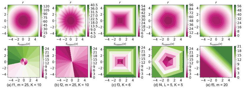
Figure 1: Visualization of test problems $f_{1}$–$f_{5}$ for dimension $n=2$. The first row shows the distribution of the ground-truth worst-case objective function $F(x)$. The second row shows the distribution of the worst-case scenario index $\operatornamewithlimits{argmax}_{s\in S}f(x,s)$ per $x$.

To test the hypotheses, we construct test problems P1–P5 below. In these problems, the number $m$ of scenarios and the number $\lvert S_{\mathrm{support}}(x^{*})\rvert$ of the support scenarios around the optimal solution $x^{*}$ of the worst-case objective $F$ are controllable. The 2D landscape of the worst-case functions $F$ and the support scenarios at each $x$ on P1–P5 are shown in Figure 1. The worst-case function in all problems is a single peak function, but each problem has a different distribution of support scenarios. All the test problems have their optimal solutions at $x^{*}=\bm{0}$ and $F(x^{*})=0$. The test problem definitions (P1–P5) are listed as follows.

1. For any $n\geqslant 2$, $m\geqslant 2$, and $K\geqslant 2$,

   $$f_{1}(x,s)=\begin{cases}\lVert x\rVert^{2}-\big{(}1+\alpha\big{)}\langle x,v_{s}\rangle^{2}&s\leqslant K\\ 2\lVert x-v_{s}\rVert^{2}-8&s>K\enspace,\end{cases}$$

   where $v_{s}=(\cos(\omega\cdot s),\sin(\omega\cdot s),0,\dots,0)$, $\alpha=(\tan\omega)^{-2}$, and $\omega=\pi/K$ for $s\leqslant K$, and $v_{s}=(\cos(\tilde{\omega}\cdot(s-K)),\sin(\tilde{\omega}\cdot(s-K)),0,\dots,0)$, $\tilde{\omega}=2\pi/(m-K)$ for $s>K$. Thus, we have $S_{\mathrm{support}}(\mathbb{R}^{n})=S$ and $S_{\mathrm{support}}(x^{*})=\{1,\dots,K\}$.

2. For any $n\geqslant 2$, $m\geqslant 2$, and $K\geqslant 2$,

   $$f_{2}(x,s)=\begin{cases}\lVert x\rVert^{2}-\big{(}1+\alpha\big{)}\langle x,v_{s}\rangle^{2}&s\leqslant K\\ \lVert x-v_{s}\rVert-2&s>K\enspace,\end{cases}$$

   where $v_{s}=(\cos(\omega\cdot s),\sin(\omega\cdot s),0,\dots,0)$, $\alpha=(\tan\omega)^{-2}$, and $\omega=\pi/K$ for $s\leqslant K$, and$v_{s}=(\cos(\tilde{\omega}\cdot(s-K)),\sin(\tilde{\omega}\cdot(s-K)),0,\dots,0)$, and $\tilde{\omega}=2\pi/(m-K)$ for $s>K$. Thus, we have that $S_{\mathrm{support}}(\mathbb{R}^{n})=S_{\mathrm{support}}(x^{*})=\{1,\dots,K\}$.

3. For any $n\geqslant 1$, $m\geqslant 2n$,

   $$f_{3}(x,s)=\langle x-\alpha_{s}\cdot v_{s},v_{s}\rangle^{2}-\beta_{s}\enspace,$$

   where $K=\lceil m/2n\rceil$, $\alpha_{s}$, $\beta_{s}$, and $v_{s}$ for each $s\in S$ are defined as follows. Let $k=\lceil s/(2\cdot n)\rceil$ and $\ell=s-2\cdot n\cdot(k-1)$. Then, $v_{s}$ is the unit vector whose $\lceil\ell/2\rceil$-th element is $(-1)^{\ell}$. We define $\tilde{\alpha}_{k}:=5\cdot k/K$, and $\tilde{\beta}_{k}:=\tilde{\beta}_{k-1}+(\tilde{\alpha}_{k}+\tilde{\alpha}_{k-1})^{2}-(2\tilde{\alpha}_{k-1})^{2}$ and $\tilde{\beta}_{1}:=\tilde{\alpha}_{1}^{2}$. Hence, we have $S_{\mathrm{support}}(\mathbb{R}^{n})=S$ and $S_{\mathrm{support}}(x^{*})=\{1,\dots,2n\}$.

4. For any $n\geqslant 1$, $m\geqslant L\geqslant 2$,

   $$f_{4}(x,s)=\lVert x\rVert^{2}+2\langle x,v_{s}\rangle-\lVert v_{s}\rVert^{2}+\frac{5}{K}\enspace,$$

   where $K=m/L$, $v_{s}=(5\cdot k/K)\cdot(\cos(\omega\cdot\ell),\sin(\omega\cdot\ell),0,\dots,0)$ for $\omega=2\pi/L$, $k=\lceil s/L\rceil$, and $\ell=s-L\cdot(k-1)$. We have $S_{\mathrm{support}}(\mathbb{R}^{n})=S$, $S_{\mathrm{support}}(x^{*})=\{1,\dots,L\}$.

5. For any $n\geqslant 1$, $m\geqslant 2$,

   $$f_{5}(x,s)=x^{2}+x\omega_{s}-\omega_{s}^{2}\enspace.$$

   where $\omega_{s}=\frac{2(s-1)}{m-1}-1$ for all $s=1,..,m$. Thus $S_{\mathrm{support}}(x^{*})=\{(m-1)/2+1\}$ if $m$ is odd, and $S_{\mathrm{support}}(x^{*})=\{m/2,m/2+1\}$ if $m$ is even.

4.2 Common Settings

We optimized P1–P5 using AS3-CMA-ES, AS3-CMA-ES with fixed $\lambda_{s}=\lvert S_{\mathrm{support}}(x^{*})\rvert$, CMA-ES and lq-CMA-ES for 20 trials with different random seeds. The search domain was $\mathbb{X}=\mathbb{R}^{n}$, with $S=\llbracket 1,m\rrbracket$. We used pycma [48] for the implementation of lq-CMA-ES. We implemented the other approaches using the version of the CMA-ES proposed in [39] as the baseline. For a fair comparison between lq-CMA-ES and the other approaches, we turned off the diagonal acceleration mechanism of [39]. All hyperparameters were set to their default values. The initial mean and covariance matrix of the CMA-ES was $m^{0}\sim\mathcal{U}(-4,4)^{n}$ and $\Sigma^{0}$ to $2^{2}\cdot I_{n}$. We used the same initial mean vector and covariance matrix for lq-CMA-ES. The other hyperparameters for lq-CMA-ES were set to their default values implemented in pycma. In these experiments, we did not perform a restart because the test problems were all single-peak problems. The hyperparameters for AS3-CMA-ES were set as follows: $c_{p}=0.3$, $\eta=0.3$, $\epsilon=1/m$, $\gamma=0.99$, and $p_{s}^{0}=0.1$ for all $s\in S$. Their sensitivities are analyzed in A. For AS3-CMA-ES with fixed $\lambda_{s}$, the hyperparameters were set as follows: $c_{p}=0.1$, $\epsilon=1/m$, $\gamma=0.99$, and $p^{0}_{s}=\lambda_{s}/m$.

The termination criteria were as follows. We regarded a run as successful if $\lvert F(m^{t})-F(x^{*})\rvert<10^{-12}$ was reached before $10^{6}$ $f$-calls were spent. If $10^{6}$ $f$-calls were spent before reaching $\lvert F(m^{t})-F(x^{*})\rvert<10^{-12}$, we regarded a run as a failure. Additionally, we implemented the following conditions: too small a search distribution $\sigma^{t}<10^{-12}$, and an excessively large condition number $\operatorname{Cond}(\Sigma^{t})>10^{14}$. If one of them was reached, we regarded the run as a failure.

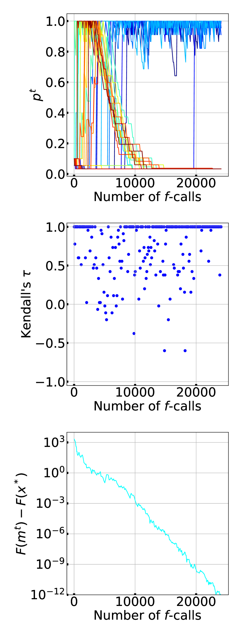
(a) P1

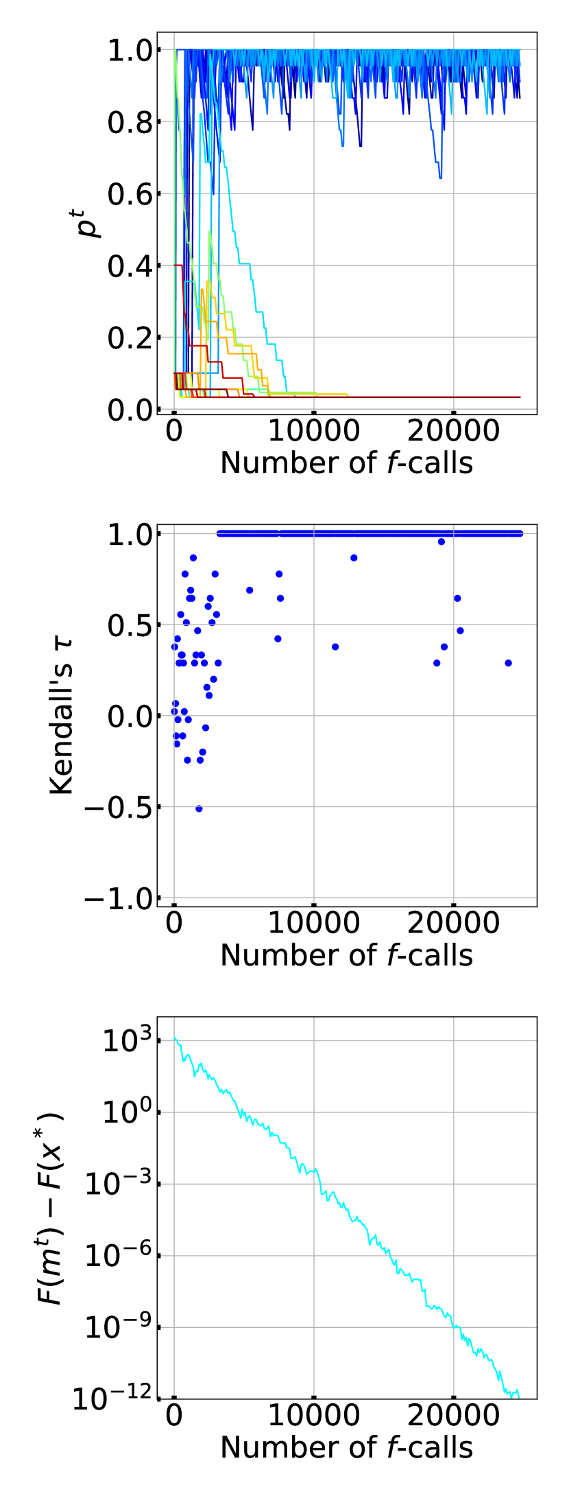
(b) P2

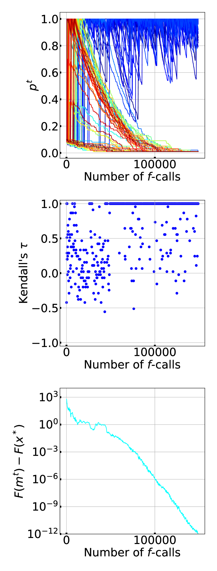
(c) P3

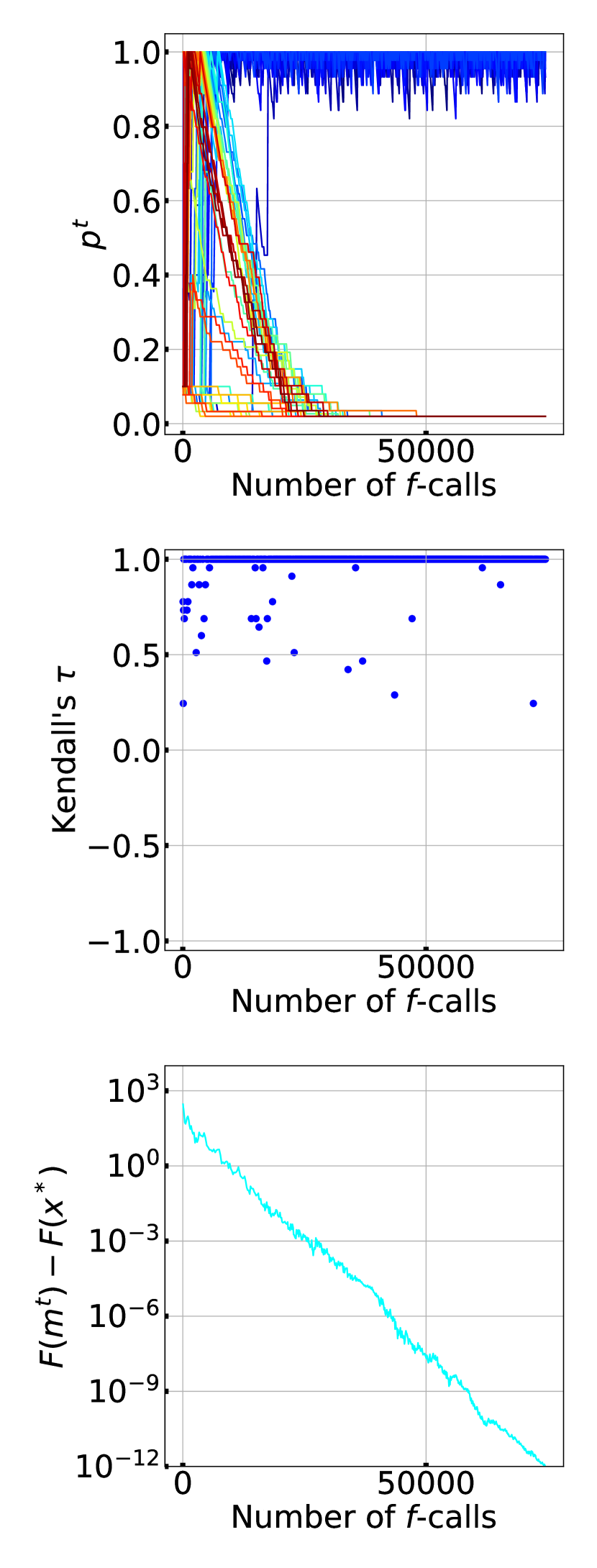
(d) P4

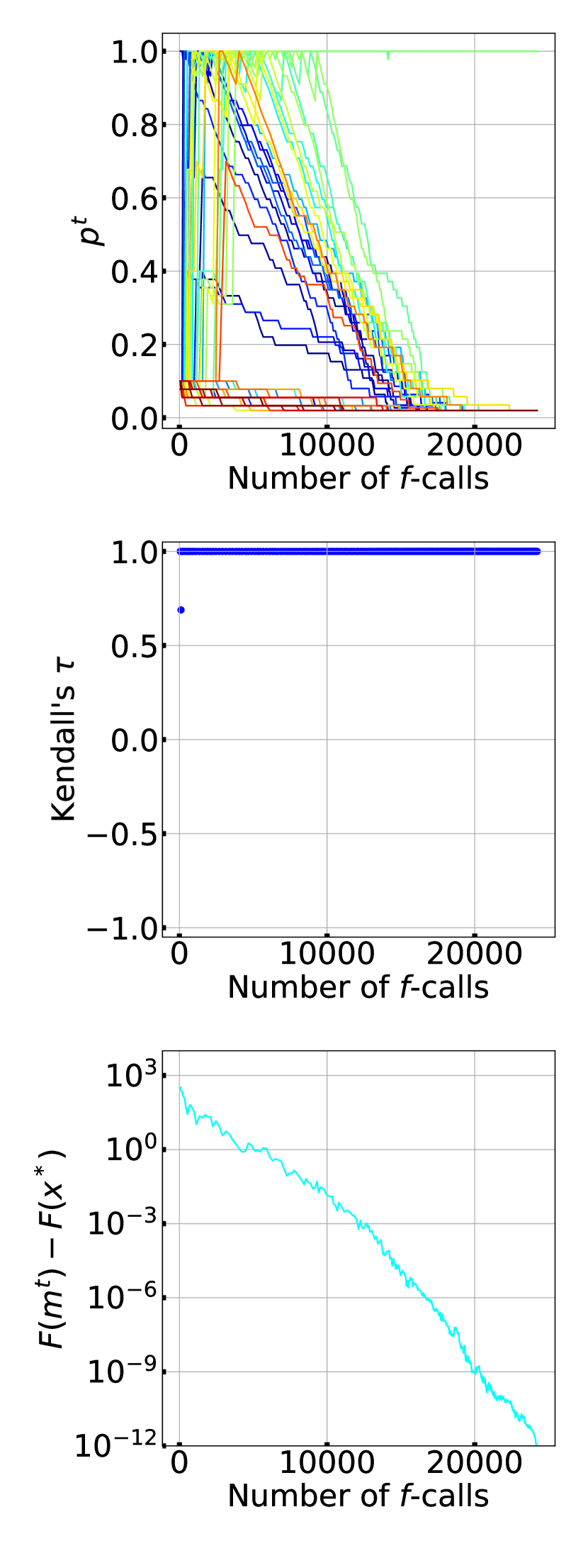
(e) P5

Figure 2: History of probability $p^{t}_{s}$, Kendall’s $\tau$, and the gap $F(m^{t})-F(x^{*})$ in a typical run on P1–P5. Curves for higher scenario indices are depicted in warmer colors.

4.3 Adaptive Behavior of $p_{s}^{t}$ in AS3-CMA-ES (Hypothesis (1))

To test Hypothesis (1), we applied AS3-CMA-ES to P1–P5 with $n=10$. The problem control parameters were set as follows: $m=30$ and $K=10$ for P1 and P2, $K=5$ (hence, $m=100$) for P3, $L=10$ and $K=5$ (hence, $m=50$) for P4 and $m=50$ (hence, $\lvert S_{\mathrm{support}}(x^{*})\rvert=2$) for P5.

Figure 2 shows the history of $p^{t}_{s}$ for each $s\in S$, the Kendall rank correlation coefficient $\tau$ between $F(x^{t}_{1}),\dots,F(x^{t}_{\lambda_{x}})$ and $F(x^{t}_{1};A^{t}),\dots,F(x^{t}_{\lambda_{x}};A^{t})$, and the gap $F(m^{t})-F(x^{*})$ in a typical optimization run for each problem. All the runs were successfully terminated by reaching the target threshold for $F$. The results for all cases show that $p^{t}_{s}$ tended to $\mathbb{I}\{s\in S_{\mathrm{support}}(x^{*})\}$ at the end of the run, and Kendall’s $\tau$ remained at one at a high frequency. P2 has the property that only $K$ scenarios can be support scenarios over the entire domain. Therefore, we see from Figure 2(b) that AS3-CMA-ES mistakenly increased $p_{s}^{t}$ for a few scenarios that are not in $S_{\mathrm{support}}(H_{\gamma}^{t})$ at the beginning. However, their $p_{s}^{t}$ values started to decrease after a few iterations. P1 has the property that it is identical to P2 around $x^{*}$, but outside the neighborhood of $x^{*}$, the support scenarios are $S\setminus S_{\mathrm{support}}(x^{*})$. In Figure 2(a), it can be observed that $p_{s}^{t}$ were increased for $s\notin S_{\mathrm{support}}(x^{*})$ initially, and $p_{s}^{t}$ subsequently began to decrease for $s\notin S_{\mathrm{support}}(x^{*})$, whereas $p_{s}^{t}$ started to increase for $s\in S_{\mathrm{support}}(x^{*})$, where we observed relatively low $\tau$ values. When iterations of low $\tau$ values continued, the reduction rate of the gap $F(m^{t})-F(x^{*})$ decreased. Similar behaviors were observed on P3–P5, where the support scenarios $S_{\mathrm{support}}(H_{\gamma}^{t})$ change gradually as $H_{\gamma}^{t}$. From these results, we confirm that $p_{s}^{t}$ follows the change of $S_{\mathrm{support}}(H_{\gamma}^{t})$.

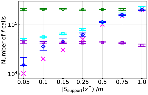
(a) P1

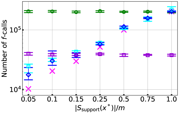
(b) P2

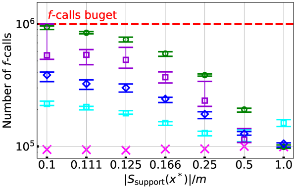
(c) P3

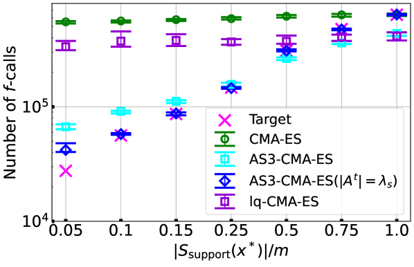
(d) P4

(e) P5

Figure 3: Comparison among CMA-ES, AS3-CMA-ES, AS3-CMA-ES with fixed $\lambda_{s}=\lvert S_{\mathrm{support}}(x^{*})\rvert$ (denoted as AS3-CMA-ES ($\lvert A^{t}\rvert=\lambda_{s}$) at the legend) and lq-CMA-ES on problems P1–P5. Mean and standard deviation of the number of $f$-calls required for convergence over 20 trials. The target is the number of $f$-calls which multiplies the average number of $f$-calls from CMA-ES and the factor $\lvert S_{\mathrm{support}}(x^{*})\rvert/m$. The ratio $\lvert S_{\mathrm{support}}(x^{*})\rvert/m$ is $K/m$ for problems P1 and P2, $1/K$ for problems P3 and P4, and $2/m$ for P5. Cases with $f$-calls reaching $10^{6}$ were evaluated as optimization failures in this experiment. CMA-ES failed at 2 trials on P3 with $\lvert S_{\mathrm{support}}(x^{*})\rvert/m=0.1$. lq-CMA-ES failed at 8, 4, and 4 trials, respectively, on P3 with $\lvert S_{\mathrm{support}}(x^{*})\rvert/m=0.1,0.111,0.125$. AS3-CMA-ES with fixed $\lambda_{s}=\lvert S_{\mathrm{support}}(x^{*})\rvert$ failed at all trials on P5. The other trials were successful.

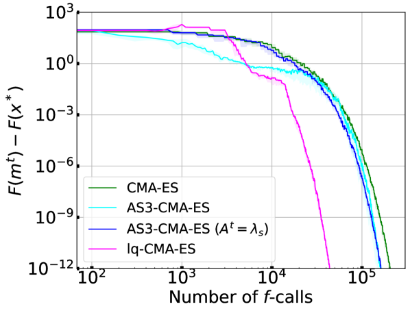
(a) $\lvert S_{\mathrm{support}}(x^{*})\rvert/m=0.75$ on P1

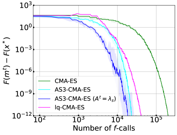
(b) $\lvert S_{\mathrm{support}}(x^{*})\rvert/m=0.05$ on P2

Figure 4: Gap $F(m^{t})-F(x^{*})$ of each approach. Solid line: median (50 percentile) over 20 runs. Shaded area: interquartile range (25–75 percentile) over 20 runs.

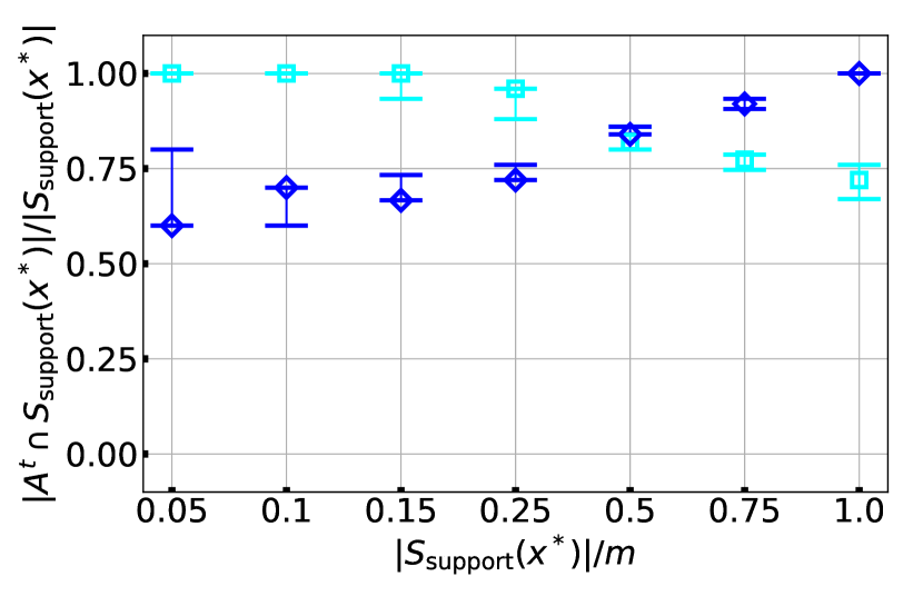
(a) P1

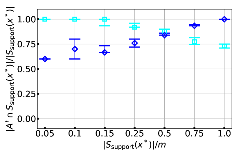
(b) P2

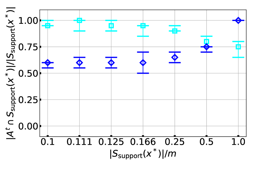
(c) P3

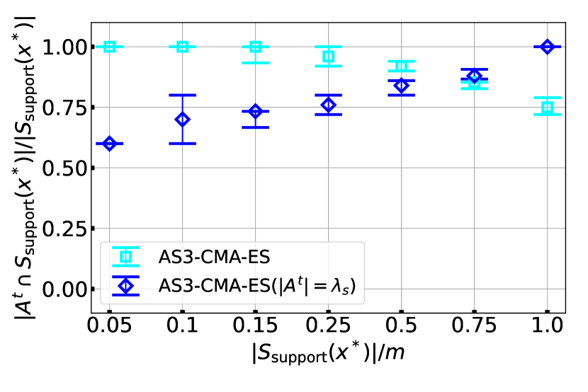
(d) P4

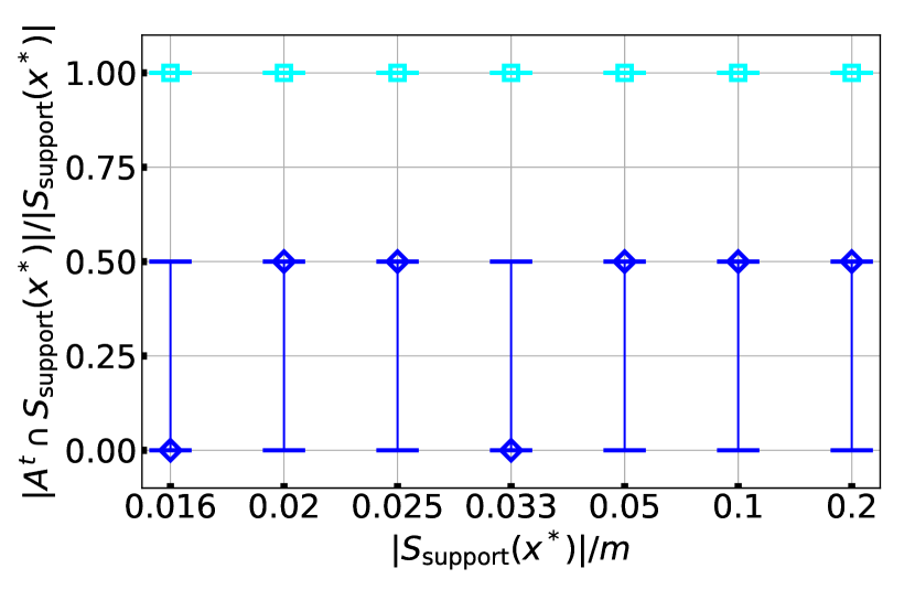
(e) P5

Figure 5: Mean and standard deviation of the ratio $\lvert A^{t}\cap S_{\mathrm{support}}(x^{*})\rvert/\lvert S_{\mathrm{support}}(x^{*})\rvert$ at the end of optimization resulted from AS3-CMA-ES and AS3-CMA-ES with fixed $\lambda_{s}=\lvert S_{\mathrm{support}}(x^{*})\rvert$ (denoted as AS3-CMA-ES ($\lvert A^{t}\rvert=\lambda_{s}$) at the legend) on problems P1–P5 over 20 trials.

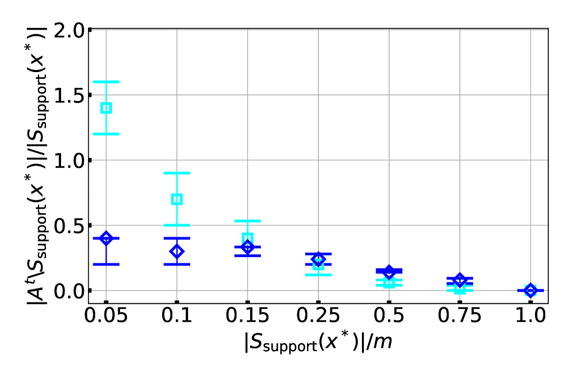
(a) P1

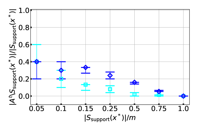
(b) P2

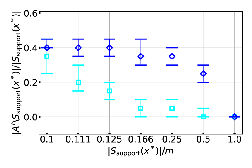
(c) P3

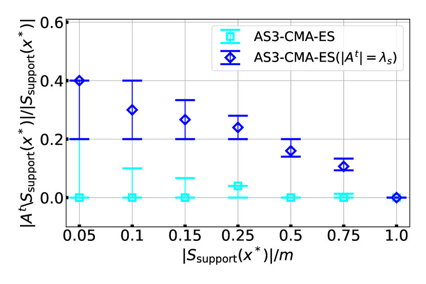
(d) P4

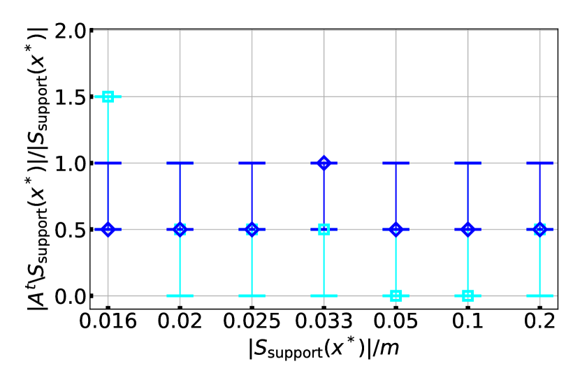
(e) P5

Figure 6: Mean and standard deviation of the ratio $\lvert A^{t}\setminus S_{\mathrm{support}}(x^{*})\rvert/\lvert S_{\mathrm{support}}(x^{*})\rvert$ at the end of optimization resulted from AS3-CMA-ES and AS3-CMA-ES with fixed $\lambda_{s}=\lvert S_{\mathrm{support}}(x^{*})\rvert$ (denoted as AS3-CMA-ES ($\lvert A^{t}\rvert=\lambda_{s}$) at the legend) on problems P1–P5 over 20 trials.

4.4 Comparison (Hypotheses (2)–(4))

To compare the four approaches with different $m$ and different $\lvert S_{\mathrm{support}}(x^{*})\rvert$ (to test Hypotheses (2)–(4)), we set the problem control parameters as follows. We set $m=100$ and $K=\{5,15,25,50,75,100\}$ for P1 and P2, $m=\{20,40,80,120,160,180,200\}$ (hence $K=\{1,2,4,6,8,9,10\}$, respectively) for P3, $L=\{5,10,15,25,50,75,100\}$ and $m=100$ for P4 and $m=\{10,20,40,60,80,100,120\}$ for P5. The problem dimension was $n=10$. The scalability of AS3-CMA-ES against $n$ and $m$ was also tested; the results are presented in B.

The comparison results are shown in Figure 3. The average and standard deviation of the number of $f$-calls until the target objective value $\lvert F(m^{t})-F(x^{*})\rvert<10^{-12}$ was reached are displayed. If optimization failed, the run was treated as a case in which $10^{6}$ $f$-calls were exhausted. As a reference, we also plotted the number of $f$-calls made by CMA-ES times the ratio $\lvert S_{\mathrm{support}}(x^{*})\rvert/m$. Additionally, Figure 4 shows the changes of gap $F(m^{t})-F(x^{*})$ obtained by four approaches on P1 with $\lvert S_{\mathrm{support}}(x^{*})\rvert/m=0.75$ and P2 with $\lvert S_{\mathrm{support}}(x^{*})\rvert/m=0.05$. To support the statistical significance of the differences in Figure 3, Table 1 shows the $p$-values from Mann–Whitney’s $U$-test between the number of $f$-calls spent by AS3-CMA-ES and that of the other approaches on each problem.To ascertain the number of support scenarios correctly selected in $A^{t}$ and the number of non-support scenarios wrongly selected in $A^{t}$, the ratios $\lvert A^{t}\cap S_{\mathrm{support}}(x^{*})\rvert/\lvert S_{\mathrm{support}}(x^{*})\rvert$ and $\lvert A^{t}\setminus S_{\mathrm{support}}(x^{*})\rvert/\lvert S_{\mathrm{support}}(x^{*})\rvert$ at the end of trials of AS3-CMA-ES and AS3-CMA-ES with fixed $\lambda_{s}=\lvert S_{\mathrm{support}}(x^{*})\rvert$ on each problem are visualized in Figure 5 and Figure 6. CMA-ES and lq-CMA-ES always use all scenarios and $\lvert A^{t}\cap S_{\mathrm{support}}(x^{*})\rvert/\lvert S_{\mathrm{support}}(x^{*})\rvert=1$ and $\lvert A^{t}\setminus S_{\mathrm{support}}(x^{*})\rvert/\lvert S_{\mathrm{support}}(x^{*})\rvert=m/\lvert S_{\mathrm{support}}(x^{*})\rvert-1$, therefore their results are omitted.

Table 1: The $p$-values from Mann–Whitney’s $U$-test between the number of $f$-calls spent by AS3-CMA-ES and that of the other approaches on each problem. The total number of tests is $105$; hence, the Bonferroni correction of the statistical significance $\alpha$ is $\alpha/105>9.5\times 10^{-5}$ for $\alpha=10^{-2}$. The difference in Figure 3 is regarded as statistically significant with $\alpha=10^{-2}$ if the corresponding $p$-value is smaller than $9.5\times 10^{-5}$.

P1
	0.05	0.1	0.15	0.25	0.5	0.75	1.0
CMA-ES	$6.73\times 10^{-8}$	$6.71\times 10^{-8}$	$6.72\times 10^{-8}$	$6.75\times 10^{-8}$	$6.64\times 10^{-8}$	$1.42\times 10^{-7}$	$4.68\times 10^{-2}$
AS3-CMA-ES with fixed $\lambda_{s}$	$6.79\times 10^{-8}$	$1.48\times 10^{-3}$	$4.6\times 10^{-4}$	$1.06\times 10^{-7}$	$1.48\times 10^{-1}$	$9.25\times 10^{-1}$	$4.38\times 10^{-2}$
lq-CMA-ES	$7.39\times 10^{-6}$	$6.74\times 10^{-8}$	$6.77\times 10^{-8}$	$6.79\times 10^{-8}$	$6.79\times 10^{-8}$	$6.77\times 10^{-8}$	$6.80\times 10^{-8}$
P2
	0.05	0.1	0.15	0.25	0.5	0.75	1.0
CMA-ES	$6.77\times 10^{-8}$	$6.70\times 10^{-8}$	$6.75\times 10^{-8}$	$6.73\times 10^{-8}$	$6.77\times 10^{-8}$	$2.74\times 10^{-4}$	$3.36\times 10^{-4}$
AS3-CMA-ES with fixed $\lambda_{s}$	$2.23\times 10^{-2}$	$9.89\times 10^{-1}$	$1.33\times 10^{-2}$	$4.38\times 10^{-2}$	$9.03\times 10^{-3}$	$2.61\times 10^{-1}$	$4.15\times 10^{-5}$
lq-CMA-ES	$6.80\times 10^{-8}$	$2.06\times 10^{-6}$	$3.05\times 10^{-4}$	$6.71\times 10^{-8}$	$6.76\times 10^{-8}$	$6.74\times 10^{-8}$	$6.79\times 10^{-8}$
P3
	0.1	0.111	0.125	0.166	0.25	0.5	1.0
CMA-ES	$6.77\times 10^{-8}$	$6.71\times 10^{-8}$	$6.73\times 10^{-8}$	$6.78\times 10^{-8}$	$1.20\times 10^{-6}$	$1.38\times 10^{-6}$	$6.77\times 10^{-8}$
AS3-CMA-ES with fixed $\lambda_{s}$	$6.79\times 10^{-8}$	$6.79\times 10^{-8}$	$6.80\times 10^{-8}$	$7.90\times 10^{-8}$	$2.59\times 10^{-5}$	$1.93\times 10^{-2}$	$6.79\times 10^{-8}$
lq-CMA-ES	$6.28\times 10^{-8}$	$6.77\times 10^{-8}$	$6.76\times 10^{-8}$	$6.79\times 10^{-8}$	$1.20\times 10^{-6}$	$6.92\times 10^{-7}$	$2.36\times 10^{-6}$
P4
	0.05	0.1	0.15	0.25	0.5	0.75	1.0
CMA-ES	$6.75\times 10^{-8}$	$6.78\times 10^{-8}$	$6.77\times 10^{-8}$	$6.79\times 10^{-8}$	$6.77\times 10^{-8}$	$6.79\times 10^{-8}$	$6.78\times 10^{-8}$
AS3-CMA-ES with fixed $\lambda_{s}$	$1.20\times 10^{-6}$	$6.76\times 10^{-8}$	$6.80\times 10^{-8}$	$3.70\times 10^{-5}$	$6.74\times 10^{-8}$	$6.75\times 10^{-8}$	$6.77\times 10^{-8}$
lq-CMA-ES	$6.80\times 10^{-8}$	$6.80\times 10^{-8}$	$6.80\times 10^{-8}$	$6.80\times 10^{-8}$	$6.79\times 10^{-8}$	$2.24\times 10^{-4}$	$1.33\times 10^{-1}$
P5
	0.016	0.02	0.025	0.033	0.05	0.1	0.2
CMA-ES	$6.74\times 10^{-8}$	$6.78\times 10^{-8}$	$6.76\times 10^{-8}$	$6.77\times 10^{-8}$	$6.76\times 10^{-8}$	$6.76\times 10^{-8}$	$6.73\times 10^{-8}$
AS3-CMA-ES with fixed $\lambda_{s}$	$7.98\times 10^{-9}$	$8.01\times 10^{-9}$	$8.01\times 10^{-9}$	$7.99\times 10^{-9}$	$8.01\times 10^{-9}$	$7.99\times 10^{-9}$	$8.01\times 10^{-9}$
lq-CMA-ES	$6.78\times 10^{-8}$	$6.80\times 10^{-8}$	$6.80\times 10^{-8}$	$6.79\times 10^{-8}$	$6.79\times 10^{-8}$	$6.79\times 10^{-8}$	$6.80\times 10^{-8}$

AS3-CMA-ES vs CMA-ES (Hypothesis (2))

Figure 3 shows that AS3-CMA-ES spent fewer $f$-calls than CMA-ES in most cases. In particular, AS3-CMA-ES was more efficient when $\lvert S_{\mathrm{support}}(x^{*})\rvert/m$ was smaller. When $\lvert S_{\mathrm{support}}(x^{*})\rvert/m\leqslant 0.25$, as shown in Figure 5 and Figure 6, $\lvert A^{t}\cap S_{\mathrm{support}}(x^{*})\rvert/\lvert S_{\mathrm{support}}(x^{*})\rvert$ resulting from AS3-CMA-ES was close to $1$, and $\lvert A^{t}\setminus S_{\mathrm{support}}(x^{*})\rvert/\lvert S_{\mathrm{support}}(x^{*})\rvert$ was relatively small in comparison with the ratio $\lvert A^{t}\setminus S_{\mathrm{support}}(x^{*})\rvert/\lvert S_{\mathrm{support}}(x^{*})\rvert=m/\lvert S_{\mathrm{support}}(x^{*})\rvert-1$ of CMA-ES (for example, in case of $m/\lvert S_{\mathrm{support}}(x^{*})\rvert=0.05$, $m/\lvert S_{\mathrm{support}}(x^{*})\rvert-1$ is $19$). These results implicitly support that AS3-CMA-ES could approximate the worst-case objective function without sampling all scenarios at the convergence. By contrast, if $\lvert S_{\mathrm{support}}(x^{*})\rvert/m\approx 1$, AS3-CMA-ES is designed to obtain similar results to those of CMA-ES, and the advantage of AS3-CMA-ES over CMA-ES was reduced.

AS3-CMA-ES vs AS3-CMA-ES with fixed $\lambda_{s}=\lvert S_{\mathrm{support}}(x^{*})\rvert$(Hypothesis (3))

On P1, P2, and P4, AS3-CMA-ES with $\lambda_{s}=\lvert S_{\mathrm{support}}(x^{*})\rvert$ achieved nearly ideal speed-up over CMA-ES, which is $\lvert S_{\mathrm{support}}(x^{*})\rvert/m$ times fewer $f$-calls (denoted as Target). For the successful convergence on P1, P2, and P4, Figure 5 shows that AS3-CMA-ES with $\lambda_{s}=\lvert S_{\mathrm{support}}(x^{*})\rvert$ needs more than half of the support scenarios at the convergence. For a relatively small $\lvert S_{\mathrm{support}}(x^{*})\rvert/m$ situation, the speed-up factor is almost ideal for P2, but it was reduced on P1 and P4. This is because $\lvert S_{\mathrm{support}}(H_{\gamma}^{t})\rvert\leqslant\lambda_{s}$ is guaranteed at P2, whereas $\lvert S_{\mathrm{support}}(H_{\gamma}^{t})\rvert$ can be greater than $\lambda_{s}$, and the support scenarios can change over time on P1 and P4 until the search distribution is sufficiently concentrated around $x^{*}$. This, as well as the time required for the adaptation of $p_{s}^{t}$, may be the reason for non-ideal speed-up. On P3, this defect was observed even for a relatively high ratio $\lvert S_{\mathrm{support}}(x^{*})\rvert/m$. On P5, $\lambda_{s}=\lvert S_{\mathrm{support}}(x^{*})\rvert=2$ was too small to approximate the worst-case objective; hence, the optimization failed.

We observe that the efficiency of AS3-CMA-ES is competitive or slightly worse than that of AS3-CMA-ES with fixed $\lambda_{s}=\lvert S_{\mathrm{support}}(x^{*})\rvert$ on P1, P2, and P4. This is a promising result, as AS3-CMA-ES with fixed $\lambda_{s}=\lvert S_{\mathrm{support}}(x^{*})\rvert$ exhibited nearly ideal performance, and AS3-CMA-ES achieved competitive performance without knowing $\lvert S_{\mathrm{support}}(x^{*})\rvert$. On P3 and P5, AS3-CMA-ES exhibited even better performance than AS3-CMA-ES with fixed $\lambda_{s}=\lvert S_{\mathrm{support}}(x^{*})\rvert$, where the number $\lvert S_{\mathrm{support}}(H_{\gamma}^{t})\rvert$ of the support scenarios in the search area $H_{\gamma}^{t}$ may be significantly greater than $\lvert S_{\mathrm{support}}(x^{*})\rvert$ and changes over time. The adaptive behavior of the number $\lvert A^{t}\rvert$ of subsampled scenarios is helpful for such situations.

AS3-CMA-ES vs lq-CMA-ES(Hypothesis (4))

lq-CMA-ES achieved a speed-up of factor $2$ to $3$ over CMA-ES, independently on the ratio $\lvert S_{\mathrm{support}}(x^{*})\rvert/m$. Therefore, if $\lvert S_{\mathrm{support}}(x^{*})\rvert/m$ is relatively small, AS3-CMA-ES is a better choice than lq-CMA-ES, whereas if $\lvert S_{\mathrm{support}}(x^{*})\rvert/m$ is relatively high, (in particular when $\lvert S_{\mathrm{support}}(x^{*})\rvert/m=1$), lq-CMA-ES is a better choice than AS3-CMA-ES. This tendency is also observed in Figure 4. However, there are also cases such as on P4 and P5 where AS3-CMA-ES is significantly better than lq-CMA-ES even when the ratio $\lvert S_{\mathrm{support}}(x^{*})\rvert/m$ is close to $1$. By contrast, AS3-CMA-ES is more advantageous as the ratio $\lvert S_{\mathrm{support}}(x^{*})\rvert/m$ is lower.

5 Application to Well Placement Optimization

We demonstrate the usefulness of AS3-CMA-ES in comparison with CMA-ES and lq-CMA-ES for well placement optimization for carbon dioxide capture and storage (CCS) with multiple geological models.

5.1 Problem Description

The problem is to optimize the placement of three injection wells to maximize the injectable $\mathrm{CO_{2}}$ volume. The objective function is the total injection volume of $\mathrm{CO_{2}}$ from the three wells. The design variable $x=(x_{1},x_{2},x_{3})$ is the 2D coordinate, where $x_{i}=(w_{1}^{i},w_{2}^{i})$ is the coordinate of the placement of the $i$th well. The problem dimension is $n=6$.

We consider obtaining a robust well placement for the uncertainty of the geological property distribution (e.g., porosity or permeability distribution). The uncertainty of the geological property distribution is worth considering because the performance of injection wells greatly depends on the geological properties of their location. In this experiment, we created $m=50$ models with different geological property distributions to represent geological uncertainty. The total injectable $\mathrm{CO_{2}}$ volume through three wells varies for different models. Here, each model is considered for each scenario, and the objective function value for the $s$th model is $f(x,s)$.

The optimization problem is formulated as the following max–min problem

$$\operatornamewithlimits{argmax}_{x\in\mathbb{X}}F(x),\quad\text{where}\quad F(x)=\min_{s=1,\cdots,m}f(x,s)\enspace.$$ (15)

Here, $F(x)$ is the minimum injectable $\mathrm{CO_{2}}$ volume among the $m$ models.

We formulated the objective function as follows. Let $f_{i,j,s}$ be the injectable $\mathrm{CO_{2}}$ volume in model $s$ at a single injection well located at $(i,j)$ for $i=1,\dots,50$ and $j=1,\dots,50$. We computed $f_{i,j,s}$ by performing numerical simulations, which amounted to 125,000 simulations in total. Let $f_{b}(\check{x},s)$ be the approximated injectable $\mathrm{CO_{2}}$ volume in model $s$ at a single injection well located at $\check{x}\in[1,50]^{2}$. This value is computed by the bilinear interpolation of $f_{i,j,s}$. The objective function is defined as follows.

$$f(x,s)=\sum_{i=1}^{3}f_{b}(x_{i:C},s)\prod_{j=1}^{i-1}(1-\exp(-d(x_{i:3},x_{j:3})))\enspace,$$ (16)

where $x_{i:3}$ is the well coordinate with the $i$th greatest injectable $\mathrm{CO_{2}}$ volume $f_{b}(x_{i:3},s)$, i.e., $f_{b}(x_{1:3},s)\geqslant f_{b}(x_{2:3},s)\geqslant f_{b}(x_{3:3},s)$, and $d(\check{y},\check{z})$ represents the distance between well $\check{y}$ and well $\check{z}$. The rationale behind (16) is as follows. First, the total injectable $\mathrm{CO_{2}}$ volume $f(x,s)$ must be no less than the injectable $\mathrm{CO_{2}}$ volume $f_{b}(x_{i},s)$ from each injection well. Second, $f(x,s)$ must be less than the sum of the injectable $\mathrm{CO_{2}}$ volume from each well when there is only one well because of the pressure interference between the wells. That is, we require $\max_{i=1,2,3}f_{s}(x_{i},s)<f(x,s)<\sum_{i=1}^{3}f_{s}(x_{i},s)$. Our objective function (16) reflects this requirement, where the pressure interference is represented by $\prod_{j=1}^{i-1}(1-\exp(-d(x_{i:3},x_{j:3})))$.

Figure 8 visualizes the injectable $\mathrm{CO_{2}}$ volume at the worst case, $\max_{s=1,\dots,m}f_{b}(\check{x},s)$, when there is only one injection well and the support scenario at each location, $\check{x}$. All the scenarios were included in the support scenarios $S_{\mathrm{support}}([1,50]^{2})$ over the search space. However, if we focus on the neighborhood of a local maximum, e.g., $\check{x}\approx(20,20)$, the number of support scenarios is no greater than 10. We expect that this characteristic is inherited by $f$. Based on the results observed in Section 4, we expect that AS3-CMA-ES is more efficient than lq-CMA-ES because the ratio $S_{\mathrm{support}}(x^{*})/m$ is relatively small.

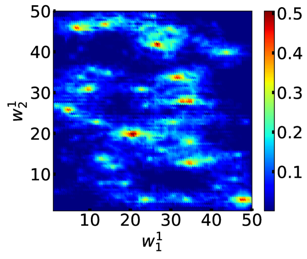
(a) $\max_{s\in S}f_{b}(x_{1},s)$

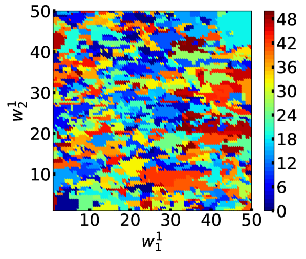
(b) $\operatornamewithlimits{argmax}_{s\in S}f_{b}(x_{1},s)$

Figure 7: Visualization of the optimization problem.

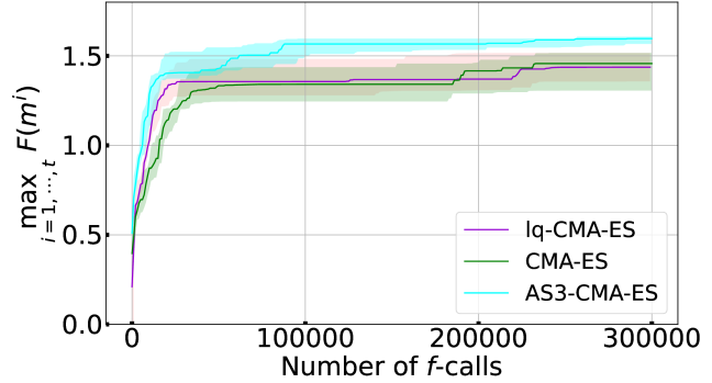
Figure 8: Best-so-far worst-case objective value $\max_{i=1,\dots,t}F(m^{i})$. Solid line: median (50 percentile) over 20 runs; Shaded area: interquartile range (25–75 percentile range) over 20 runs.

5.2 Experimental Settings

We applied AS3-CMA-ES, CMA-ES, and lq-CMA-ES to this problem. The search domain was $\mathbb{X}=[1,50]^{6}$, with $S=\llbracket 1,50\rrbracket$. We used pycma for the implementation of lq-CMA-ES. We implemented other approaches using the version of the CMA-ES proposed in [39] as the baseline. For a fair comparison between lq-CMA-ES and the other approaches, we turned off the diagonal acceleration mechanism of [39]. All hyperparameters were set to their default values. The initial mean vector and covariance matrix of the CMA-ES were set as $m^{0}\sim\mathcal{U}(\mathbb{X})$ and $\Sigma^{0}=(12.5)^{2}\cdot I_{n}$. The parameters for AS3-CMA-ES were set as follows: $c_{p}=0.3$, $\eta=0.3$, $\epsilon=1/m$, $\gamma=0.99$, and $p_{s}^{0}=0.1$ for all $s\in S$. We used the same initial mean vector and covariance matrix as initial settings for lq-CMA-ES. The other hyperparameters for lq-CMA-ES were set to their default values implemented in pycma.

In this experiment, we employed a simple restart strategy with default $\lambda_{x}$ to deal with multimodality. The termination condition for restart was an excessively small coordinate-wise standard deviation $\max_{i=1,\dots,n}\Sigma^{t}_{i,i}<10^{-8}$, where $\Sigma^{t}_{i,i}$ is the $i$th diagonal element of the covariance matrix $\Sigma^{t}$. If this condition was satisfied, the mean vector and covariance matrix were initialized as $m^{0}\sim\mathcal{U}(\mathbb{X})$ and $\Sigma^{0}=(12.5)^{2}\cdot I_{n}$, and $p_{s}^{0}=0.1$ for all $s\in S$ for AS3-CMA-ES.

We evaluated the performance of each algorithm by computing the worst-case performance $F(m^{t})$ evaluated at the mean vector $m^{t}$ at each iteration. We performed 20 independent trials for each algorithm with a maximum of $f$-calls of $3\times 10^{5}$.

5.3 Results and Analysis

Figure 8 shows the median (50 percentile) and interquartile range (25–75 percentile range) of the best-so-far worst-case performance values $\max_{i=1,\dots,t}F(m^{i})$. As a summary of the computational results, the median and interquartile range of the best-so-far worst-case performance values at the end of the optimization and $p$-values against AS3-CMA-ES resulting from Mann–Whitney’s $U$-test are shown in Table 2. Figure 9 shows the history of the worst-case performance at each iteration of each algorithm on a typical trial. The sharp drops of $F(m^{t})$ indicate restarts of the algorithms. Figure 11 shows the history of the sum $\sum_{s=1}^{m}p_{s}^{t}$ of the sampling probability of scenarios in AS3-CMA-ES on a typical trial. Note that this is the expected number of sampled scenarios at each iteration, i.e., $\mathbb{E}[\lvert A^{t}\rvert]$. Figure 11 shows Kendall’s $\tau$ between the ranking of the worst case objective function values $\{F(x_{i}^{t})\}_{i=1}^{\lambda_{x}}$ and the ranking of the solution candidates computed inside the algorithms, which are the ranking of $\{F(x_{i}^{t};A^{t})\}$ in AS3-CMA-ES. Higher values indicate higher correlations between the true and estimated values.

AS3-CMA-ES vs CMA-ES

Figure 8 and Table 2 show that AS3-CMA-ES outperformed CMA-ES. AS3-CMA-ES obtained higher $50$ percentile values of $\max_{t}F(m^{t})$ from the beginning of the optimization, and smaller interquartile ranges at $300,000$ $f$-calls. We consider this to be because AS3-CMA-ES performed more restarts within the fixed budget of $f$-calls, as may be noted from Figure 9. Because the worst-case objective has multiple local optima, restarts are essential to obtain a better local optimum. AS3-CMA-ES performed more restarts because it saves $f$-calls for each restart by subsampling a scenario subset, whose cardinality decreased to around $10$ at the end of each restart (see Figure 11). The smaller interquartile range can also be attributed to the greater number of restarts because the best among more local maxima have less variation than the best among fewer local maxima.

Table 2: Median and interquartile range of best-so-far worst-case objective value over 20 runs at the end of the optimization, and $p$-values from Mann–Whitney’s $U$-test on the best-so-far worst-case values obtained by AS3-CMA-ES and CMA-ES at $100,000$, $200,000$, and $300,000$ $f$-calls. The number of tests is $6$; hence, the Bonferroni correction of the statistical significance $\alpha$ is $\alpha/6>1.66\times 10^{-3}$ for $\alpha=10^{-2}$, indicating that all the results were statistically significant with $\alpha=10^{-2}$.

Approach	Median	Interquartile range	$p$-values against AS3-CMA-ES
	300,000 $f$-calls	300,000 $f$-calls	100,000 $f$-calls	200,000 $f$-calls	300,000 $f$-calls
AS3-CMA-ES	$1.60$	$0.04$	–	–	–
CMA-ES	$1.46$	$0.21$	$1.06\times 10^{-2}$	$1.79\times 10^{-4}$	$1.25\times 10^{-5}$
lq-CMA-ES	$1.44$	$0.16$	$1.12\times 10^{-3}$	$1.38\times 10^{-6}$	$1.20\times 10^{-6}$

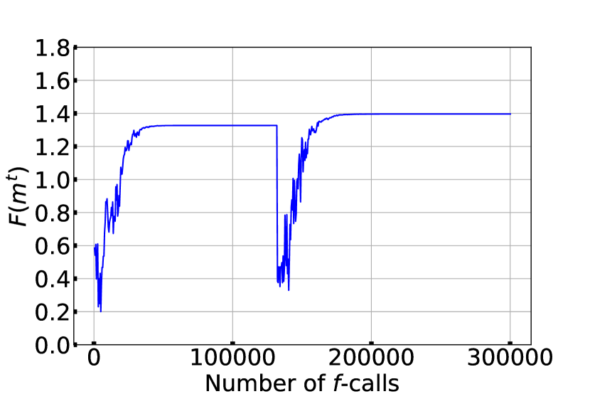
(a) CMA-ES

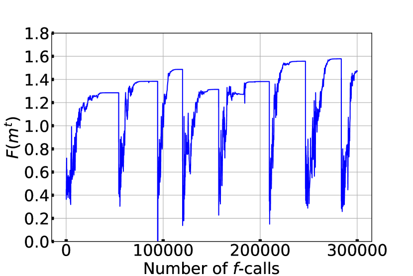
(b) AS3-CMA-ES

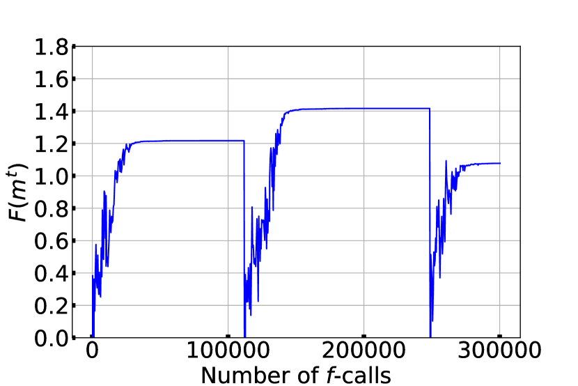
(c) lq-CMA-ES

Figure 9: History of $F(m^{t})$ in a typical run for each algorithm.

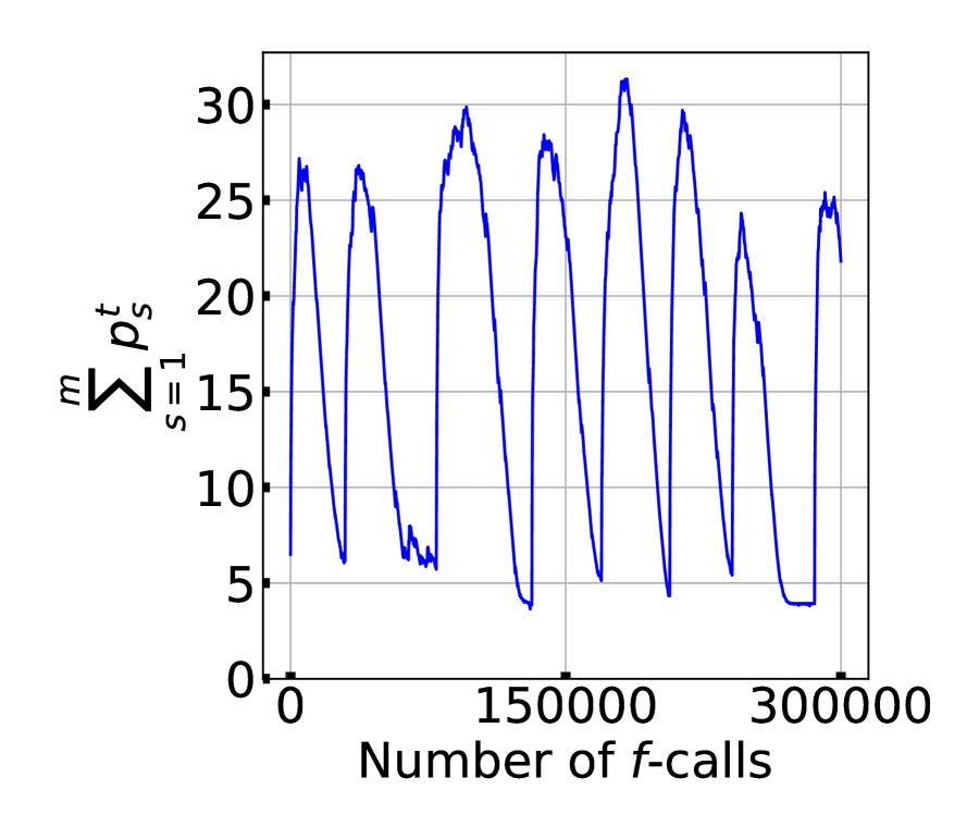
Figure 10: History of $\mathbb{E}[\lvert A^{t}\rvert]=\sum_{s=1}^{m}p^{t}_{s}$ on a typical run of AS3-CMA-ES.

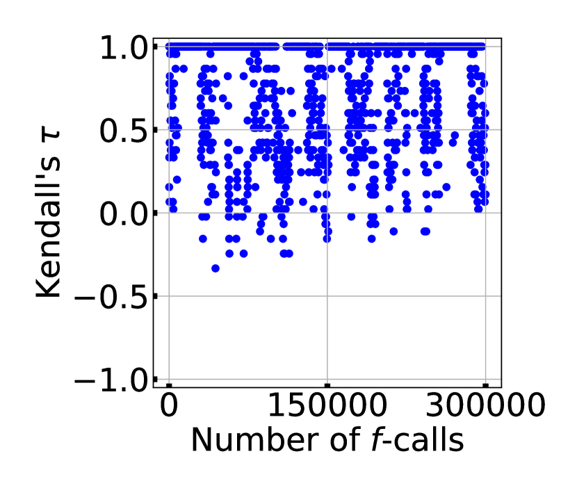
(a) AS3-CMA-ES

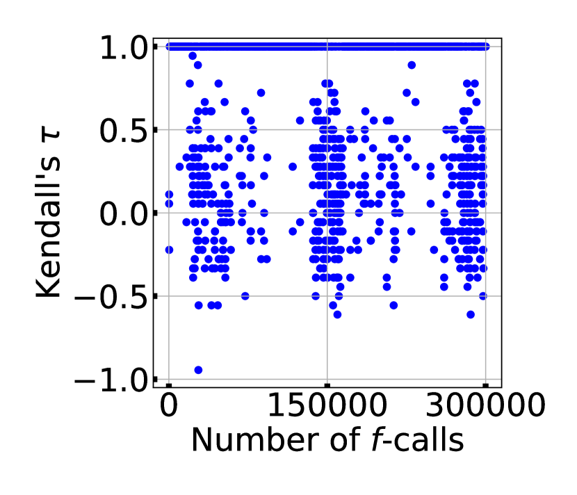
(b) lq-CMA-ES

Figure 11: History of Kendall’s $\tau$ between the rankings of the solution candidates based on the worst-case objective function values and the ranking computed inside each algorithm in a typical run.

AS3-CMA-ES vs lq-CMA-ES

Figure 8 and Table 2 show that AS3-CMA-ES outperformed lq-CMA-ES. As shown in Figure 8, AS3-CMA-ES obtained higher $50$ percentile values than lq-CMA-ES from the beginning of the optimization, and smaller interquartile ranges at $300,000$ $f$-calls. Similarly to the advantage of AS3-CMA-ES over CMA-ES, AS3-CMA-ES was able to perform more restarts than lq-CMA-ES, whereas lq-CMA-ES performed more restarts than CMA-ES on average. That is, AS3-CMA-ES converged to a local optimum faster than lq-CMA-ES for each restart. The reason may be twofold. First, the ratios $\lvert S_{\mathrm{support}}(\hat{x})\rvert/m$ around the local optima $\hat{x}$ are sufficiently small for AS3-CMA-ES to be more efficient than lq-CMA-ES. As confirmed in the previous sections, the efficiency of AS3-CMA-ES over CMA-ES was greater when this ratio was smaller, whereas the efficiency of lq-CMA-ES over CMA-EX was virtually constant. In this problem, the ratio $\lvert A^{t}\rvert/m$ decreased by approximately $1/5$ in AS3-CMA-ES, as shown in Figure 11. Second, the surrogate model inside lq-CMA-ES, which is a linear-quadratic model, may not be suitable for this problem, possibly because of multimodality and non-smoothness. As may be noted from Figure 11, the rank correlation between the true worst-case values and the output of the surrogate model tends to be frequently lower than $0$. If it is smaller than the predefined threshold, lq-CMA-ES spends $f$-calls to train the surrogate model. Therefore, Figure 11 indicates that lq-CMA-ES frequently updates the surrogate model by spending $f$-calls, resulting in a slower convergence than AS3-CMA-ES.

6 Conclusions

We targeted the worst-case optimization with a finite scenario set $S=\{1,\cdots,m\}$, and the objective function values were evaluated using computationally expensive numerical simulations. In this study, we focused on reducing the number of simulation executions (referred to as $f$-calls for simplicity) for the objective function value of the problem. The conclusions of this study are summarized as follows.

1. The definition of support scenarios $S_{\mathrm{support}}(H)$ at a neighborhood $H$ was introduced to elucidate the idea of approximating the worst-case objective function without sampling every possible scenario. We designed five test problems in which we could control the number of support scenarios around the optimal solution.

2. We proposed a new optimization algorithm, denoted adaptive scenario subset selection CMA-ES (AS3-CMA-ES), which optimizes continuous variables vector $x$ by the CMA-ES while approximating the worst-case objective function $F$ by adaptively subsampling a set of support scenarios in the current search area.

3. Numerical experiments were conducted on test problems to compare AS3-CMA-ES with a brute-force approach (Algorithm 1) and a surrogate-assisted approach lq-CMA-ES. We confirmed that AS3-CMA-ES generally outperformed the brute-force approach. Moreover, AS3-CMA-ES outperformed lq-CMA-ES when the ratio of the number of support scenarios to the total number of scenarios was relatively small (e.g., $<1/3$).

4. The effectiveness of AS3-CMA-ES was demonstrated on well placement optimization problems. AS3-CMA-ES was able to obtain a better well placement than lq-CMA-ES and the brute-force approach because of more frequent restarts due to the greater efficiency of AS3-CMA-ES compared to the other approaches.

In this study, numerical experiments on benchmark problems with various characteristics were not conducted. Five benchmark problems were considered, and the worst-case objective function in all of them was a single-peak function. Therefore, in future work, the performance of the proposed approach should be investigated on benchmark problems whose worst-case objective function is ill-conditioned, multimodal, or has variable dependencies.

Another direction of future work is to combine AS3-CMA-ES and the approaches smoothing the worst-case objective function. As introduced in Section 1.3, the worst-case objective function becomes naturally non-smooth owing to its construction. We expect that the CMA-ES for minimization can become more efficient by smoothing the worst-case objective function obtained by AS3.

Appendix A Sensitivity Analysis

The sensitivities of AS3-CMA-ES on $\eta$, $c_{p}$, $p^{0}$, and $\epsilon$ were investigated to demonstrate the effect of these hyperparameters and the robustness of the proposed approach. Unless otherwise specified, we followed the experimental setting described in Section 4.2, except for the maximum number of $f$-calls, which was set to $2\times 10^{6}$ in this analysis.

The test problems were set as follows. $n=10$ for all problems, $K=\{5,10,15,25,50,75,100\}$ and $m=100$ for P1 and P2, $m=\{20,40,80,120,160,180,200\}$ (hence, $K=\{1,2,4,6,8,9,10\}$) for P3, $L=\{5,10,15,25,50,75,100\}$ and $m=100$ for P4. They were set to test the performance of AS3-CMA-ES on different ratios $S_{\mathrm{support}}(x^{*})/m$.

A.1 Sensitivity to $\eta$

A higher $\eta$, and hence a higher $c_{n}$, is expected to require fewer $f$-calls to decrease $p_{s}^{t}$ for $s\notin S_{\mathrm{support}}(H^{t}_{\gamma})$. However, a higher $\eta$ has a risk of not increasing $p_{s}^{t}$ for $s\in S_{\mathrm{support}}(H_{\gamma}^{t})$, which does not satisfy condition (9).

The results on P3 and P4 are shown in Figure 12. We observed a tendency on P1 and P2 similar to that observed on P3, and hence they are omitted.

The results for P3 show that a higher $\eta$ converges faster when $\lvert S_{\mathrm{support}}(x^{*})\rvert/m$ is relatively small, such as $0.1$. A higher $\eta$ contributes to a faster decrease in $p^{t}_{s}$ for each $s\notin S_{\mathrm{support}}(H^{t}_{\gamma})$ to avoid sampling unnecessary scenarios. However, when $\lvert S_{\mathrm{support}}(x^{*})\rvert/m$ on P3 increases, a higher $\eta$ requires more $f$-calls. Additionally, setting $\eta\geqslant 0.7$ led to the optimization failure when $\lvert S_{\mathrm{support}}(x^{*})\rvert/m=1.0$. This occurred because a high $\eta$ decreased the number of support scenarios whose $p^{t}_{s}$ was kept at a relatively high value. As a result, AS3-CMA-ES failed to sample a sufficient number of support scenarios to approximate $F$. For example, on P3 with $\lvert S_{\mathrm{support}}(x^{*})\rvert=m=20$, the expected number of sampled scenarios, i.e., $\mathbb{E}[\lvert A^{t}\rvert]=\sum^{m}_{s=1}p^{t}_{s}$, was maintained at approximately $16$ with $\eta=0.1$, whereas it was maintained at approximately $8$ with $\eta=0.9$.

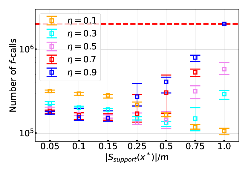
(a) P3

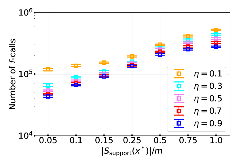
(b) P4

Figure 12: Mean and standard deviation of the number of $f$-calls over 20 trials obtained from AS3-CMA-ES with various $\eta$ on P3 and P4. The number of $f$-calls in all cases with $\eta=0.7,0.9$ on $P3$ reached $2\times 10^{6}$, and they were evaluated as optimization failures in this experiment.

By contrast, on P4, AS3-CMA-ES with a higher $\eta$ could successfully determine the optimal solution for all problem instances, and the number of $f$-calls was smaller. This is attributed to the characteristics of P4 and the comparison-based nature of CMA-ES. In contrast to P1–P3 and P5, we can select a subset $A\subset S_{\mathrm{support}}(x^{*})$ such that $\min_{x\in\mathbb{X}}F(x;A)=\min_{x\in\mathbb{X}}F(x)$ with $\lvert A\rvert=2$ or $3$. If $L$ is even or odd, $\lvert A\rvert=2$ or $3$, respectively. That is, even if $\lvert A^{t}\rvert\ll\lvert S_{\mathrm{support}}(x^{*})\rvert$, it was possible to locate the optimum of $F$ by solving $\min_{x\in\mathbb{X}}F(x;A)$, whereas $F(x)$ was not necessarily approximated well by $F(x;A^{t})$. For example, on P4 with $m=L=\lvert S_{\mathrm{support}}(x^{*})\rvert=100$, we observed that $\mathbb{E}[\lvert A^{t}\rvert]=\sum^{m}_{s=1}p^{t}_{s}$ was maintained at approximately 40–50, which is smaller than half of $\lvert S_{\mathrm{support}}(x^{*})\rvert$, while the Kendall’s $\tau$ between $F(x)$ and $F(x;A^{t})$ computed for solution candidates generated at each iteration was maintained at nearly one during the optimization. We consider that the characteristics of P4 were unusual, and note that setting $\eta$ to a small value is advisable in general.

A.2 Sensitivity to $c_{p}$

A higher $c_{p}$ is expected to result in a faster adaptation of $p_{s}^{t}$, leading to faster convergence. However, $p^{t}_{s}$ for a scenario $s\notin S_{\mathrm{support}}(x^{*})$ also increases, resulting in spending more $f$-calls. Another impact of a higher $c_{p}$ is a higher $c_{n}$ because of (12), and we have already discussed the sensitivity of $c_{n}$ in A.1.

To distinguish the effect of $c_{p}$ from the effect of $c_{n}$, we set $c_{n}=0.003$, which is the value when we set $\eta=0.1$ and $c_{p}=0.3$ for P1, P2, and P4 in this analysis.

The results are presented in Figure 13. The results for P2 and P3 showed a tendency similar to that observed for P1; hence, they are omitted. We observed that a smaller $c_{p}$ converges faster if $\lvert S_{\mathrm{support}}(x^{*})\rvert/m\lessapprox 1/2$. In the case of $\lvert S_{\mathrm{support}}(x^{*})\rvert/m\gtrapprox 1/2$, a greater $c_{p}$ tended to converge faster on P1–P3 and P5, whereas a smaller $c_{p}$ was better on P4. However, the differences in the number of $f$-calls made for $c_{p}=0.01$, $0.1$, $0.3$, and $1.0$ were at most a factor of $2$ for all cases in the experiments. Therefore, we conclude that the performance of AS3-CMA-ES is not sensitive to $c_{p}$ value.

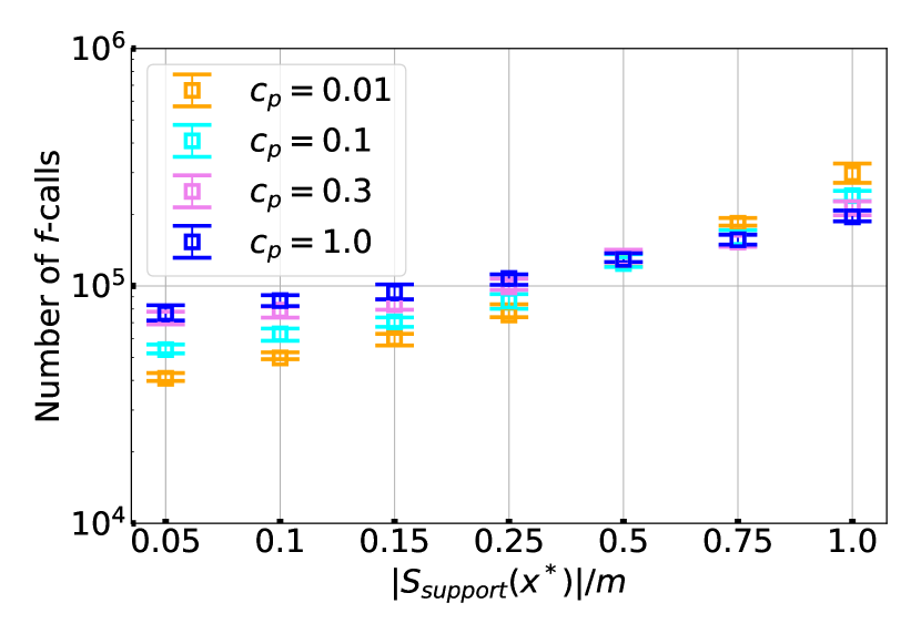
(a) $P1$

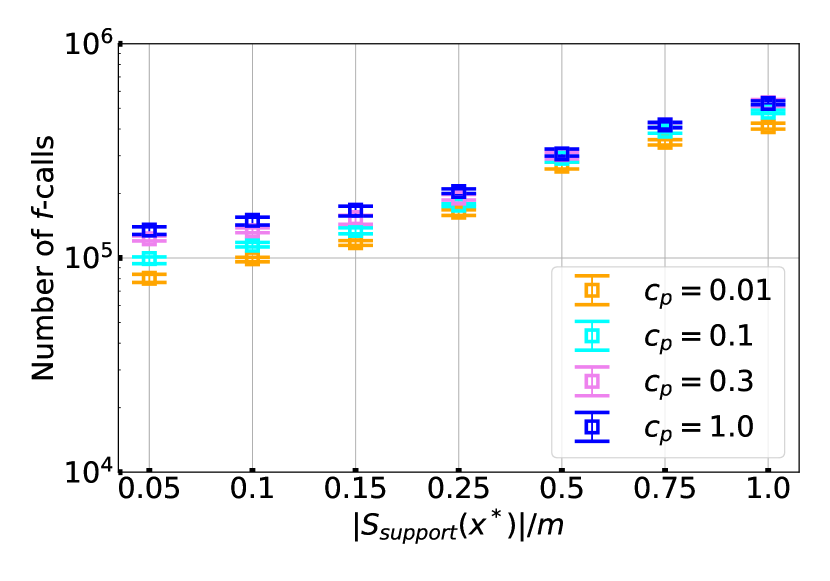
(b) P4

Figure 13: Mean and standard deviation of the number of $f$-calls over 20 trials obtained from AS3-CMA-ES with various $c_{p}$.

A.3 Sensitivity to $p^{0}$

The impact of the initial $p_{s}^{0}$ was investigated. The results are presented in Figure 14. The results for P2 and P3 showed a tendency similar to that observed for P1; hence, they are omitted.

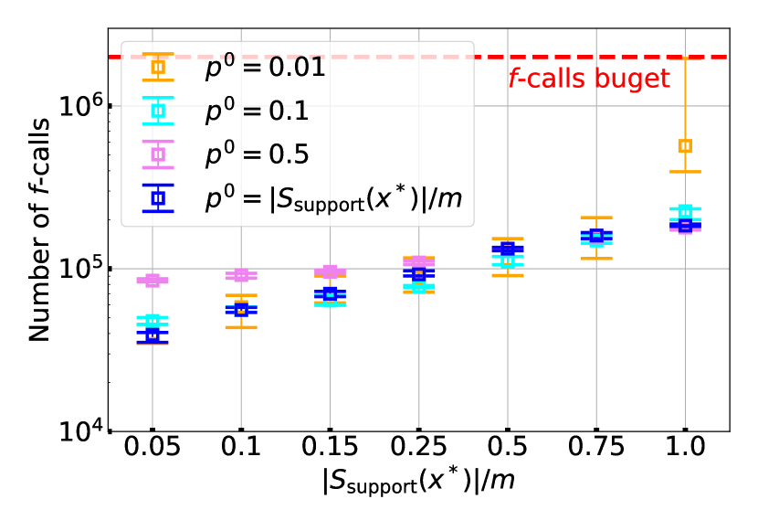
(a) P1

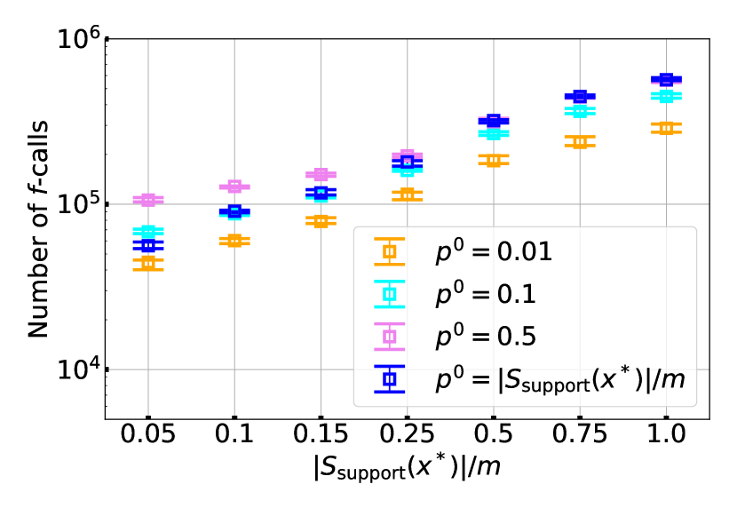
(b) P4

Figure 14: Mean and standard deviation of the number of $f$-calls over 20 trials obtained from AS3-CMA-ES with various $p^{0}$ on P1. Cases with $f$-calls reaching $2\times 10^{6}$ were evaluated as optimization failures in this experiment.

We observed the tendency that a smaller $p_{s}^{0}$ converges faster if $\lvert S_{\mathrm{support}}(x^{*})\rvert/m$ is small, whereas a larger $p_{s}^{0}$ converges faster if $\lvert S_{\mathrm{support}}(x^{*})\rvert/m$ is large for P1–P3 and P5. This is advantageous if $\mathbb{I}\{s\in S_{\mathrm{support}}(H_{\gamma}^{0})\}$ is approximated by the initial $p_{s}^{0}$, as it does not need to adapt $p_{s}^{t}$ at the beginning, thereby minimizing $f$-calls. If $p_{s}^{0}$ is set to a greater value, it requires more $f$-calls to decrease $p_{s}^{t}$ for non-support scenarios. If $p_{s}^{0}$ is set to a smaller value, more $f$-calls are required to increase $p_{s}^{t}$ for support scenarios. The experimental results reflect these expectations. On P4, we observed that a smaller $p_{s}^{0}$ resulted in a faster convergence. This is due to the characteristics of P4, as discussed above.

We note that an excessively small $p_{s}^{0}$ value sometimes leads to optimization failure. On P1 with $m=\lvert S_{\mathrm{support}}(x^{*})\rvert$, AS3-CMA-ES with $p_{s}^{0}=0.01$ failed to converge. We observed divergent behavior in the search distribution in this situation, in which $\lVert m^{t}-x^{*}\rVert$ increased to $10^{11}$ at the beginning of the search. This is possibly because the landscape of $F(x;A^{t})$ changed drastically at each iteration. Therefore, it is safer to set $p_{s}^{0}$ to a relatively high value, although doing so may reduce efficiency.

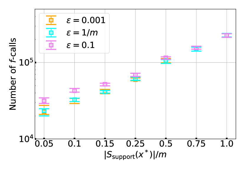
(a) P2

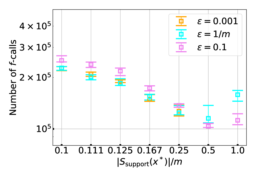
(b) P3

Figure 15: Mean and standard deviation of the number of $f$-calls over 20 trials obtained from AS3-CMA-ES with various $\epsilon$ on P2 and P3. No trials with $\epsilon=0.001$ were successful when $\lvert S_{\mathrm{support}}(x^{*})\rvert/m\geqslant 0.5$ on P3.

A.4 Sensitivity to $\epsilon$

The minimal probability $\epsilon$ is introduced to prevent $p_{s}^{t}$ from converging to $0$, resulting in the algorithm not sampling $s$ forever. With $\epsilon$, all scenarios are guaranteed to be sampled every $1/\epsilon$ iterations in expectation. However, because the expected number of sampled scenarios is $\sum_{s=1}^{m}p_{s}^{t}\geqslant\epsilon\cdot m$, this limits the upper bound of the speed-up factor over the brute-force approach. In this study, we investigated the impact of $\epsilon$.

The results are shown in Figure 15. The results for P1 and P4 showed a tendency similar to that observed on P2; hence, they are omitted.

We observed that a small $\epsilon$ required fewer $f$-calls when $\lvert S_{\mathrm{support}}(x^{*})\rvert/m$ was relatively small at P1–P4, as a small $\epsilon$ allows $\sum_{s}^{m}p^{t}_{s}$ to be as small as $\lvert S_{\mathrm{support}}(x^{*})\rvert$ at the convergence, resulting in fewer $f$-calls. We note that an excessively small $\epsilon$ led to failure in some problem instances. On P3, AS3-CMA-ES with $\epsilon=0.001$ failed to converge at $x^{*}$ when $\lvert S_{\mathrm{support}}(x^{*})\rvert/m\geqslant 0.5$. Therefore, we advise setting $\epsilon$ to a relatively high value, while the efficiency of AS3-CMA-ES may be lost.

Appendix B Scalability Analysis

The efficiency of AS3-CMA-ES for problems with higher $n$ and $m$ than those in Section 4 was investigated. Unless otherwise specified, we followed the experimental setting described in Section 4.2, except for the maximum number of $f$-calls, which was set to $2\times 10^{7}$ in this analysis.

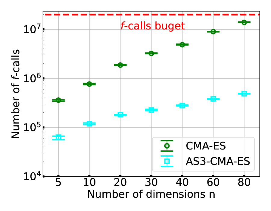
Figure 16: Mean and standard deviation of the number of $f$-calls over 20 trials with various $n$ on P4.

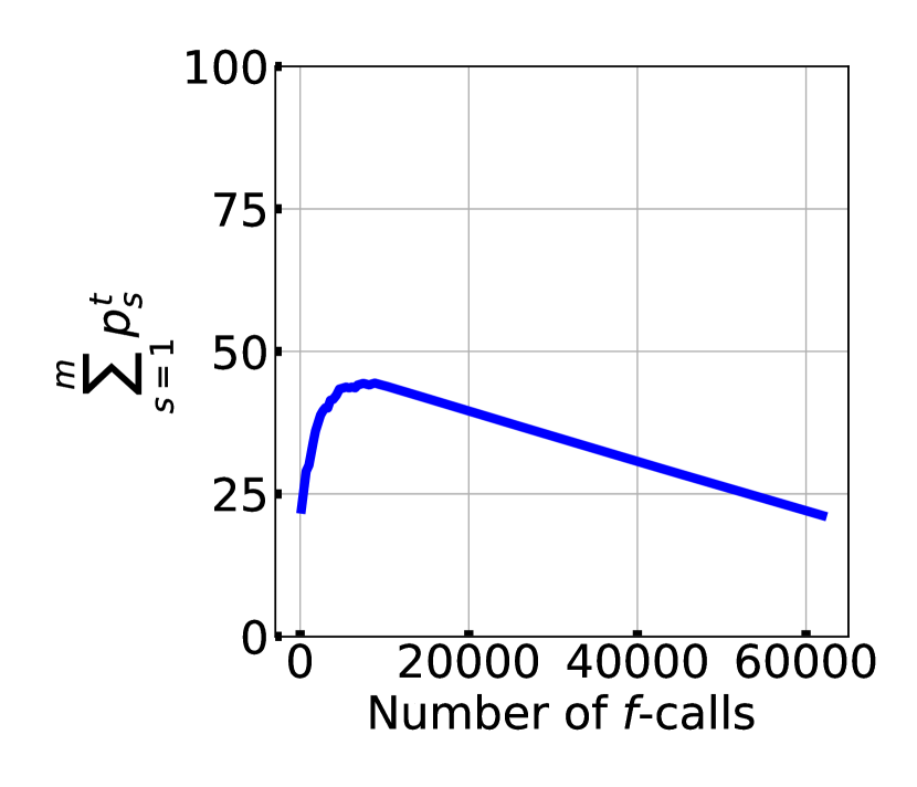
(a) $n=5$

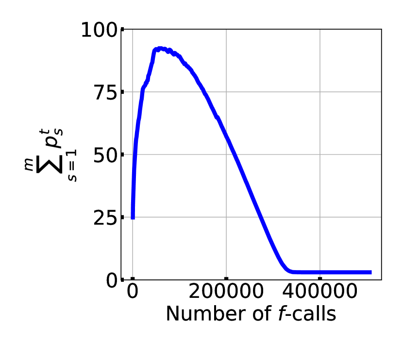
(b) $n=80$

Figure 17: History of $\sum_{s=1}^{m}p^{t}_{s}$ on a typical run on P4 ($L=2,m=200$)

B.1 Scalability to $n$

To show the effect of $n$ and the robustness of AS3-CMA-ES, we conducted a scalability analysis of $n$. For this analysis, we applied CMA-ES and AS3-CMA-ES to P1–P5 in the following problem settings to analyze the scalability of $n$. We set, $n=\{5,10,20,30,40,60,80\}$, and $K=2$ at $m=200$ for $P1$ and $f_{2}$, and $m=200$ (hence, $K=\{20,10,5,4,3,2,2\}$) for $f_{3}$, $L=2$ at $m=200$ for $f_{4}$ and $m=200$ for $f_{5}$.

The results are presented in Figure 17. The results for P1–P3 and P5 showed a tendency similar to that observed on P4; hence, they are omitted. As Figure 17 shows, both algorithms showed increased numbers of $f$-calls for convergence with increasing $n$. The efficiency of AS3-CMA-ES over CMA-ES in terms of the number of $f$-calls was at most a factor of $20$ for all the cases.

The results show that the efficiency of AS3-CMA-ES over CMA-ES was higher at a higher $n$. This is because AS3-CMA-ES on the problem with $n=80$ spent sufficient $f$-calls to learn $p^{t}_{s}$ for each $s\in S$ when approaching $x^{*}$. We confirmed that AS3-CMA-ES on the problem with $n=80$ successfully determined the optimum solution while maintaining $\sum_{s}^{m}p^{t}_{s}\approx\lvert S_{\mathrm{support}}(x^{*})\rvert$. Figure 17 shows the history of $\sum_{s}^{m}p^{t}_{s}$ resulting from a typical run with $n=5$ and $80$ on P4. The expected number of sampled scenarios, i.e., $\mathbb{E}[\lvert A^{t}\rvert]=\sum^{m}_{s=1}p^{t}_{s}$, was decreased to $\lvert S_{\mathrm{support}}(x^{*})\rvert=2$ when $n=80$, whereas it was more than $\lvert S_{\mathrm{support}}(x^{*})\rvert$ ($\sum_{s}^{m}p^{t}_{s}\approx 25$ in the end) in the case of $n=5$.

B.2 Scalability to $m$

The number of $f$-calls spent by AS3-CMA-ES depends on the number of support scenarios $\lvert S_{\mathrm{support}}(x^{*})\rvert$, whereas CMA-ES and lq-CMA-ES linearly increases the number of $f$-calls if the number of scenarios $m$ increases. Therefore, if $\lvert S_{\mathrm{support}}(x^{*})\rvert$ is fixed, AS3-CMA-ES is expected to be more efficient than CMA-ES and lq-CMA-ES for a larger $m$. However, if $m$ is larger, AS3-CMA-ES will spend more $f$-calls to adapt $p^{t}_{s}$ for each $s\in S$ to $\mathbb{I}\{s\in S_{\mathrm{support}}(H_{\gamma}^{t})\}$. On the other hand, if the ratio $\lvert S_{\mathrm{support}}(x^{*})\rvert/m$ is fixed, the efficiency of AS3-CMA-ES is expected to be even at a higher $m$.

To demonstrate the scalability to $m$ under a fixed $\lvert S_{\mathrm{support}}(x^{*})\rvert$, we applied CMA-ES , lq-CMA-ES, and AS3-CMA-ES to P1–P5. We set, $n=10$ and $m=\{20,40,80,120,160,200,240,280,320,360,400\}$ (hence, $K=\{2,4,8,12,16,\\ 20,24,28,32,36,40\}$) for $f_{3}$, and $m=\{10,20,40,80,120,160,200,240,280,320,360,400\}$ for other problems. The number $\lvert S_{\mathrm{support}}(x^{*})\rvert$ of the support scenarios was $20$ for P3 and $2$ for the others. To demonstrate the scalability to $m$ under a fixed $\lvert S_{\mathrm{support}}(x^{*})\rvert/m$, we applied CMA-ES, lq-CMA-ES, and AS3-CMA-ES to P1 and P2, respectively. We set, $n=10$ and $m=\{40,80,120,160,200,240,280,320,360,400\}$ for P1 and P2. We fixed the ratio $\lvert S_{\mathrm{support}}(x^{*})\rvert/m$ at $0.05$.

The scalability to $m$ under a fixed $\lvert S_{\mathrm{support}}(x^{*})\rvert$ is shown in Figure 19. The results for P2–P5 showed a tendency similar to that observed on P1; hence, they were omitted. The number of $f$-calls spent by CMA-ES and lq-CMA-ES increased linearly with increasing $m$, whereas lq-CMA-ES required fewer $f$-calls than CMA-ES. On the other hand, AS3-CMA-ES increased the number of $f$-calls; however, the increment in $f$-calls was less than that of CMA-ES and lq-CMA-ES. Although $S_{\mathrm{support}}(x^{*})$ was fixed, AS3-CMA-ES spent more $f$-calls by increasing $m$. We considered that more $f$-calls were spent for the adaptation of $p^{t}_{s}$ for each $s\in S$ when $m$ was set at a higher value. Figure 19 show that the efficiency of AS3-CMA-ES over CMA-ES and lq-CMA-ES was improved with increasing $m$, if $S_{\mathrm{support}}(x^{*})$ was fixed.

The scalability to $m$ under a fixed $\lvert S_{\mathrm{support}}(x^{*})\rvert/m$ is shown in Figure 19. The results for P1 showed a tendency similar to that observed for P2; hence, they were omitted. The efficiency of AS3-CMA-ES over CMA-ES was maintained until $m=400$. By contrast, the number of $f$-calls spent by lq-CMA-ES was close to that of AS3-CMA-ES. As shown in Figure 3, lq-CMA-ES showed a high efficiency for P2. We consider that it is easy for lq-CMA-ES to build a proper surrogate model for P2.

We observed that the number of $f$-calls spent by AS3-CMA-ES depends on the number of support scenarios $\lvert S_{\mathrm{support}}(x^{*})\rvert$ rather than the number of scenarios $m$, and its efficiency was maintained until $m=400$. The maximum ratio of the number of $f$-calls spent by AS3-CMA-ES and CMA-ES was approximately $10$ and that spent for AS3-CMA-ES and lq-CMA-ES was approximately $6$ for all cases in this experiment.

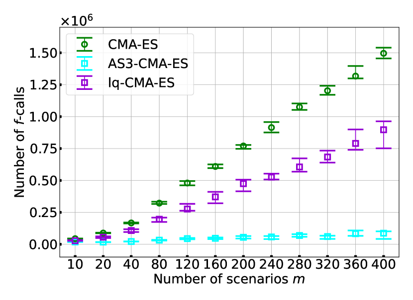
Figure 18: Mean and standard deviation of the number of $f$-calls over 20 trials with various $m$ and fixed $\lvert S_{\mathrm{support}}(x^{*})\rvert$ on P4.

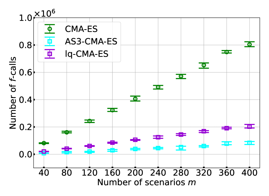
Figure 19: Mean and standard deviation of the number of $f$-calls over 20 trials with various $m$ and fixed $\lvert S_{\mathrm{support}}(x^{*})\rvert/m$ on P2.

Appendix C Effect of $\lambda_{s}$ in AS3-CMA-ES with fixed $\lambda_{s}$

The hyperparameter $\lambda_{s}$, which is the number of subsampled scenarios, is expected to have the following effects on the performance of AS3-CMA-ES with fixed $\lambda_{s}$. A higher $\lambda_{s}$ is expected to require more $f$-calls. However, a low $\lambda_{s}$ such that $\lambda_{s}\ll\lvert S_{\mathrm{support}}(x^{*})\rvert$ will struggle to converge because approximating $F$ becomes difficult. In this study, we investigated the impact of $\lambda_{s}$.

We chose P1 and P4 for analysis. P2 and P3 are the same in terms of $\lambda_{s}\geqslant\lvert S_{\mathrm{x^{*}}}\rvert$ is one of the necessary conditions to obtain a successful convergence; hence, they are omitted. On P4, in contrast to P1–P3, it is possible for AS3-CMA-ES with fixed $\lambda_{s}$ to optimize the problems if $\lambda_{s}$ is set to more than $2$ or $3$.

In this analysis, we set $n=10$ and $m=30$ with $K=15$ for $P1$ and $L=15$ for $P4$. For the other experimental settings, we followed the setting described in Section 4.2. The results are shown in Figure 20.

At P1, AS3-CMA-ES with fixed $\lambda_{s}$ converged at a lower number of $f$-calls by setting $\lambda_{s}\approx\lvert S_{\mathrm{support}}(x^{*})\rvert$. In addition, optimization was successful in some problems, even when $\lambda_{s}<\lvert S_{\mathrm{support}}(x^{*})\rvert$. This might be because the worst-case objective function $F$ was relatively well-approximated in the search neighborhood $H_{\gamma}^{t}$, as indicated by the relatively high values of Kendall’s $\tau$. However, at the settings $\lambda_{s}\ll\lvert S_{\mathrm{support}}(x^{*})\rvert$, the optimization failed because $\lambda_{s}$ was too small to approximate $F$. At P4, $\lambda_{s}\geqslant 3$ was one of the necessary conditions to obtain a successful convergence, and $\lambda_{s}\approx 3$ had the highest performance, whereas $\lambda_{s}<3$ led to failure.

Consequently, the number of $f$-calls spent by AS3-CMA-ES with fixed $\lambda_{s}$ depended on the setting of $\lambda_{s}$. Among the cases obtaining successful convergence, the ratio of the number of $f$-calls was approximately $7$ at most in this experiment. However, if $\lambda_{s}$ was too small, the optimization was considered to have failed.

(a) P1 ($\lvert S_{\mathrm{support}}(x^{*})\rvert=15$)

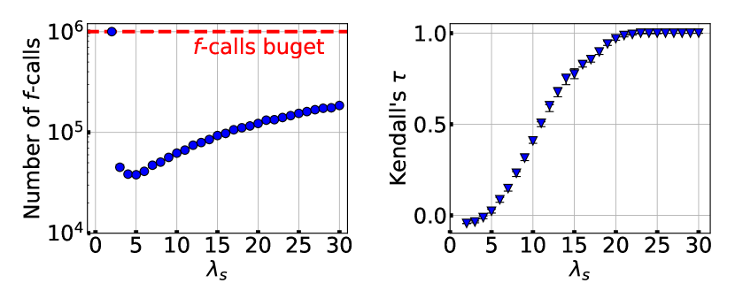
(b) P4 ($\lvert S_{\mathrm{support}}(x^{*})\rvert=15$)

Figure 20: Mean and standard deviation of the number of $f$-calls and Kendall’s $\tau$ over 20 trials obtained from AS3-CMA-ES at fixed $\lambda_{s}$ for various $\lambda_{s}$. Kendall’s $\tau$ values were averaged over the latter half of the search iterations. Cases with $f$-calls reaching $10^{6}$ were evaluated as optimization failures in this experiment.

References

- [1] D. Urieli, P. MacAlpine, S. Kalyanakrishnan, Y. Bentor, P. Stone, On optimizing interdependent skills: a case study in simulated 3d humanoid robot soccer, in: AAMAS, Vol. 11, 2011, pp. 769–776.
- [2] A. Maki, N. Sakamoto, Y. Akimoto, H. Nishikawa, N. Umeda, Application of optimal control theory based on the evolution strategy (cma-es) to automatic berthing, Journal of Marine Science and Technology 25 (1) (2020) 221–233.
- [3] D. Schafroth, C. Bermes, S. Bouabdallah, R. Siegwart, Modeling, system identification and robust control of a coaxial micro helicopter, Control Engineering Practice 18 (7) (2010) 700–711.
- [4] G. Fujii, Y. Akimoto, M. Takahashi, Exploring optimal topology of thermal cloaks by cma-es, Applied Physics Letters 112 (6) (2018) 061108.
- [5] A. L. Marsden, M. Wang, J. E. Dennis, P. Moin, Optimal aeroacoustic shape design using the surrogate management framework, Optimization and Engineering 5 (2) (2004) 235–262.
- [6] G. Hitz, E. Galceran, M.-È. Garneau, F. Pomerleau, R. Siegwart, Adaptive continuous-space informative path planning for online environmental monitoring, Journal of Field Robotics 34 (8) (2017) 1427–1449.
- [7] M. Sadeghi, M. Kalantar, Multi types dg expansion dynamic planning in distribution system under stochastic conditions using covariance matrix adaptation evolutionary strategy and monte-carlo simulation, Energy conversion and management 87 (2014) 455–471.
- [8] Z. Bouzarkouna, D. Y. Ding, A. Auger, Well placement optimization with the covariance matrix adaptation evolution strategy and meta-models, Computational Geosciences 16 (1) (2012) 75–92.
- [9] A. Miyagi, Y. Akimoto, H. Yamamoto, Well placement optimization under geological statistical uncertainty, in: Proceedings of the Genetic and Evolutionary Computation Conference, GECCO ’19, Association for Computing Machinery, New York, NY, USA, 2019, pp. 1284–1292. doi:10.1145/3321707.3321736.
-
[10]
D. Ha, J. Schmidhuber,
Recurrent
world models facilitate policy evolution, in: S. Bengio, H. Wallach,
H. Larochelle, K. Grauman, N. Cesa-Bianchi, R. Garnett (Eds.), Advances in
Neural Information Processing Systems, Vol. 31, Curran Associates, Inc.,
2018.
URL https://proceedings.neurips.cc/paper/2018/file/2de5d16682c3c35007e4e92982f1a2ba-Paper.pdf - [11] P. Chrabaszcz, I. Loshchilov, F. Hutter, Back to basics: Benchmarking canonical evolution strategies for playing atari, in: Proceedings of the 27th International Joint Conference on Artificial Intelligence, IJCAI’18, AAAI Press, 2018, p. 1419–1426.
- [12] V. Volz, J. Schrum, J. Liu, S. M. Lucas, A. Smith, S. Risi, Evolving mario levels in the latent space of a deep convolutional generative adversarial network, in: Proceedings of the genetic and evolutionary computation conference, 2018, pp. 221–228.
-
[13]
T. Tanabe, K. Fukuchi, J. Sakuma, Y. Akimoto,
Level generation for angry
birds with sequential vae and latent variable evolution, in: Proceedings of
the Genetic and Evolutionary Computation Conference, GECCO ’21, Association
for Computing Machinery, New York, NY, USA, 2021, p. 1052–1060.
doi:10.1145/3449639.3459290.
URL https://doi.org/10.1145/3449639.3459290 -
[14]
M. Nomura, S. Watanabe, Y. Akimoto, Y. Ozaki, M. Onishi,
Warm starting
cma-es for hyperparameter optimization, Proceedings of the AAAI Conference
on Artificial Intelligence 35 (10) (2021) 9188–9196.
URL https://ojs.aaai.org/index.php/AAAI/article/view/17109 -
[15]
N. Hansen, A. Auger, R. Ros, S. Finck, P. Pošík,
Comparing results of 31
algorithms from the black-box optimization benchmarking bbob-2009, in:
Proceedings of the 12th Annual Conference Companion on Genetic and
Evolutionary Computation, GECCO ’10, Association for Computing Machinery, New
York, NY, USA, 2010, p. 1689–1696.
doi:10.1145/1830761.1830790.
URL https://doi.org/10.1145/1830761.1830790 - [16] A. Miyagi, H. Yamamoto, Y. Akimoto, Z. Xue, Parallel workflow to optimize well placement in heterogeneous reservoir using covariance matrix adaptation evolution strategy, GHGT-14, 2018.
- [17] IPCC, Carbon dioxide capture and storage, Tech. rep., Cambridge University Press, UK (2005).
-
[18]
B. Yeten, L. J. Durlofsky, K. Aziz,
Optimization of nonconventional well
type, location, and trajectory, SPE Journal 8 (03) (2003) 200–210.
doi:10.2118/86880-PA.
URL https://doi.org/10.2118/86880-PA -
[19]
L. Durlofsky, I. Aitokhuehi, V. Artus, B. Yeten, K. Aziz,
Optimization
of advanced well type and performance, 9th European Conference on the
Mathematics of Oil Recovery, 2004.
doi:https://doi.org/10.3997/2214-4609-pdb.9.B031.
URL https://www.earthdoc.org/content/papers/10.3997/2214-4609-pdb.9.B031 -
[20]
V. Artus, L. J. Durlofsky, J. Onwunalu, K. Aziz,
Optimization of
nonconventional wells under uncertainty using statistical proxies,
Computational Geosciences 10 (4) (2006) 389–404.
doi:10.1007/s10596-006-9031-9.
URL https://doi.org/10.1007/s10596-006-9031-9 -
[21]
A. H. Alhuthali, A. D. Gupta, B. Yuen, J. P. Fontanilla,
Optimizing
smart well controls under geologic uncertainty, Journal of Petroleum Science
and Engineering 73 (1) (2010) 107 – 121.
doi:https://doi.org/10.1016/j.petrol.2010.05.012.
URL http://www.sciencedirect.com/science/article/pii/S0920410510001099 - [22] H. Yamamoto, S. Nanai, K. Zhang, P. Audigane, C. Chiaberge, R. Ogata, N. Nishikawa, Y. Hirokawa, S. Shingu, K. Nakajima, Numerical simulation of long-term fate of co2 stored in deep reservoir rocks on massively parallel vector supercomputer, in: High Performance Computing for Computational Science - VECPAR 2012, Springer, 2013, pp. 80–92.
-
[23]
G. Liuzzi, S. Lucidi, M. Sciandrone, A
derivative-free algorithm for linearly constrained finite minimax problems,
SIAM Journal on Optimization 16 (4) (2006) 1054–1075.
arXiv:https://doi.org/10.1137/040615821, doi:10.1137/040615821.
URL https://doi.org/10.1137/040615821 -
[24]
C. Bogani, M. G. Gasparo, A. Papini,
Generating set search methods for
piecewise smooth problems, SIAM Journal on Optimization 20 (1) (2009)
321–335.
arXiv:https://doi.org/10.1137/070708032, doi:10.1137/070708032.
URL https://doi.org/10.1137/070708032 -
[25]
H. Warren, M. Mason,
Derivative-free
optimization methods for finite minimax problems, Optimization Methods and
Software 28 (2) (2013) 300–312.
arXiv:https://doi.org/10.1080/10556788.2011.638923, doi:10.1080/10556788.2011.638923.
URL https://doi.org/10.1080/10556788.2011.638923 -
[26]
P. R. Ballin, A. G. Journel, K. Aziz,
Prediction of uncertainty in
reservoir performance forecast, Journal of Canadian Petroleum Technology
31 (04).
doi:10.2118/92-04-05.
URL https://doi.org/10.2118/92-04-05 -
[27]
D. R. Fenik, A. Nouri, C. V. Deutsch,
Criteria for ranking realizations in
the investigation of sagd reservoir performance, pETSOC-2009-191 (2009).
doi:10.2118/2009-191.
URL https://doi.org/10.2118/2009-191 -
[28]
Ranking Geostatistical Realizations by
Measures of Connectivity, SPE International Thermal Operations and Heavy
Oil Symposium, sPE-98168-MS.
arXiv:https://onepetro.org/SPEITOHOS/proceedings-pdf/05ITOHOS/All-05ITOHOS/SPE-98168-MS/1841075/spe-98168-ms.pdf,
doi:10.2118/98168-MS.
URL https://doi.org/10.2118/98168-MS - [29] C. Scheidt, J. Caers, Representing spatial uncertainty using distances and kernels, Math. Geosci. 41 (2009) 397–419. doi:10.1007/s11004-008-9186-0.
-
[30]
C. Scheidt, J. Caers, Uncertainty
quantification in reservoir performance using distances and kernel
methods–application to a west africa deepwater turbidite reservoir, SPE
Journal 14 (04) (2009) 680–692.
doi:10.2118/118740-PA.
URL https://doi.org/10.2118/118740-PA -
[31]
C. Scheidt, J. Caers,
Bootstrap confidence
intervals for reservoir model selection techniques, Computational
Geosciences 14 (2) (2010) 369–382.
doi:10.1007/s10596-009-9156-8.
URL https://doi.org/10.1007/s10596-009-9156-8 - [32] Z. Li, C. A. Floudas, Optimal scenario reduction framework based on distance of uncertainty distribution and output performance: I. single reduction via mixed integer linear optimization, Computers and Chemical Engineering 70 (2014) 50 – 66. doi:https://doi.org/10.1016/j.compchemeng.2014.03.019.
- [33] S. Rahim, Z. Li, J. Trivedi, Reservoir geological uncertainty reduction: an optimization-based method using multiple static measures, Math Geosci 47 (2015) 373–396.
- [34] A.Zhou, Q.Zhang, A surrogate-assisted evolutionary algorithm for minimax optimization, in: IEEE Congress on Evolutionary Computation, 2010, pp. 1–7. doi:10.1109/CEC.2010.5586122.
- [35] H.Wang, Y. Jin, J. O. Jansen, Data-driven surrogate-assisted multiobjective evolutionary optimization of a trauma system, IEEE Transactions on Evolutionary Computation 20 (6) (2016) 939–952. doi:10.1109/TEVC.2016.2555315.
-
[36]
T. B. Beielstein, M. Zaefferer,
Model-based
methods for continuous and discrete global optimization, Applied Soft
Computing 55 (2017) 154–167.
doi:https://doi.org/10.1016/j.asoc.2017.01.039.
URL https://www.sciencedirect.com/science/article/pii/S1568494617300546 -
[37]
N. Hansen, A global surrogate
assisted cma-es, in: Proceedings of the Genetic and Evolutionary Computation
Conference, GECCO ’19, Association for Computing Machinery, New York, NY,
USA, 2019, p. 664–672.
doi:10.1145/3321707.3321842.
URL https://doi.org/10.1145/3321707.3321842 - [38] A. Miyagi, K. Fukuchi, J. Sakuma, Y. Akimoto, Adaptive scenario subset selection for min–max black-box continuous optimization, in: Proceedings of the Genetic and Evolutionary Computation Conference, GECCO ’21, Association for Computing Machinery, New York, NY, USA, 2021.
- [39] Y. Akimoto, N. Hansen, Diagonal acceleration for covariance matrix adaptation evolution strategies, Evolutionary Computation 28 (3) (2020) 405–435.
- [40] N. Hansen, A. Auger, Principled Design of Continuous Stochastic Search: From Theory to Practice, Springer Berlin Heidelberg, Berlin, Heidelberg, 2014, pp. 145–180.
-
[41]
N. Hansen, A. Ostermeier,
Completely derandomized
self-adaptation in evolution strategies, Evol. Comput. 9 (2) (2001)
159–195.
doi:10.1162/106365601750190398.
URL https://doi.org/10.1162/106365601750190398 - [42] L. M. Rios, N. V. Sahinidis, Derivative-free optimization: a review of algorithms and comparison of software implementations, Journal of Global Optimization 56 (3) (2013) 1247–1293.
- [43] N. Hansen, S. Kern, Evaluating the cma evolution strategy on multimodal test functions, in: Parallel Problem Solving from Nature - PPSN VIII, Springer Berlin Heidelberg, Berlin, Heidelberg, 2004, pp. 282–291.
- [44] A. Auger, H. Hansen, A restart cma evolution strategy with increasing population size, in: Proceedings of 2005 IEEE Congress on Evolutionary Computation, CEC ’05, IEEE, 2005, pp. 1769–1776. doi:10.1109/CEC.2005.1554902.
-
[45]
N. Hansen, Benchmarking a
bi-population cma-es on the bbob-2009 function testbed, in: Proceedings of
the 11th Annual Conference Companion on Genetic and Evolutionary Computation
Conference: Late Breaking Papers, GECCO ’09, Association for Computing
Machinery, New York, NY, USA, 2009, p. 2389–2396.
doi:10.1145/1570256.1570333.
URL https://doi.org/10.1145/1570256.1570333 -
[46]
Y. Akimoto, Y. Nagata, I. Ono, S. Kobayashi,
Theoretical foundation for
cma-es from information geometry perspective, Algorithmica 64 (4) (2012)
698–716.
doi:10.1007/s00453-011-9564-8.
URL https://doi.org/10.1007/s00453-011-9564-8 -
[47]
Y. Akimoto, T. Shimizu, T. Yamaguchi,
Adaptive objective selection
for multi-fidelity optimization, in: Proceedings of the Genetic and
Evolutionary Computation Conference, GECCO ’19, Association for Computing
Machinery, New York, NY, USA, 2019, p. 880–888.
doi:10.1145/3321707.3321709.
URL https://doi.org/10.1145/3321707.3321709 - [48] N. Hansen, Y. Akimoto, P. Baudis, Cma-es/pycma on github, Zenodo 10. doi:10.5281/zenodo.2559634.