Relative Sparsity for Medical Decision Problems

Abstract

Existing statistical methods can estimate a policy, or a mapping from covariates to decisions, which can then instruct decision makers (e.g., whether to administer hypotension treatment based on covariates blood pressure and heart rate). There is great interest in using such data-driven policies in healthcare. However, it is often important to explain to the healthcare provider, and to the patient, how a new policy differs from the current standard of care. This end is facilitated if one can pinpoint the aspects of the policy (i.e., the parameters for blood pressure and heart rate) that change when moving from the standard of care to the new, suggested policy. To this end, we adapt ideas from Trust Region Policy Optimization (TRPO). In our work, however, unlike in TRPO, the difference between the suggested policy and standard of care is required to be sparse, aiding with interpretability. This yields “relative sparsity,” where, as a function of a tuning parameter, $\lambda$, we can approximately control the number of parameters in our suggested policy that differ from their counterparts in the standard of care (e.g., heart rate only). We propose a criterion for selecting $\lambda$, perform simulations, and illustrate our method with a real, observational healthcare dataset, deriving a policy that is easy to explain in the context of the current standard of care. Our work promotes the adoption of data-driven decision aids, which have great potential to improve health outcomes.

1 Introduction

Although risk models for mortality and morbidity are commonly used in the healthcare setting, decision models, which can provide guidance with respect to which treatment to choose, are not. Much in the way that risk models can help providers and patients determine prognosis, decision models can help providers and patients make better, or even optimal, treatment decisions. There has therefore been great interest in the statistics and machine learning communities on developing methodology to estimate decision models from data. ⁴; ⁴⁷; ¹⁸ For example, authors have developed methods with applications to the management of hypotension, ¹⁸; ²¹ sepsis, ⁵⁸ and diabetes. ¹³; ⁴³ However, there remains a major barrier to widespread adoption of decision models: it is sometimes difficult to justify to decision-makers why they should replace the established standard of care, or their “behavioral policy,” with a new, suggested policy. In this work, we provide methodology for deriving policies that are easy to explain in the context of the standard of care, and whose adoption is therefore easy to justify.

To develop policies that are easy to explain in the context of the standard of care, we build on the policy search framework, ⁵¹; ⁷⁰ in which one defines a reward function and attempts to find a policy that will maximize it directly. In order to perform policy search, one uses importance sampling ⁵³; ⁷¹ or policy gradients ,⁷⁰ which are equivalent to certain techniques in inverse probability weighting. ²⁹; ⁶⁰; ⁴ Policy search differs from Q-learning and model based reinforcement learning, where the value function and transition probabilities are modeled, respectively. ⁷⁶; ⁶⁵; ¹⁵ In policy search, one specifies a model only for the policy, and the expected reward is optimized directly as a function of the policy parameters. This is convenient when one wishes to place a constraint on the policy itself, as we will in the current work.

Our work is related to Trust Region Policy Optimization (TRPO), ⁶⁴ where one maximizes some reward, but also requires that the suggested policy be in some sense close to the data-generating behavioral policy. In the current literature, TRPO is primarily applied to non-medical problems, such as updating a robot’s behavior without taking too large of a step. In the robotics setting, since one can simply change the code by which a machine behaves, there is no need to justify a change in policies. Hence, in TRPO, the difference between the suggested and behavioral policies is a black box; there is no requirement that the policies be parameterized, and if they are, there is no guarantee that the difference between the parameters of the two policies be interpretable. In healthcare, however, it is important to explain to patients and providers why they should shift from their current policy, which is the standard of care, to a new policy. To this end, our main methodological development is a relative sparsity penalty on the parameters of the suggested and behavioral policies. We aim to provide a suggested policy such that there is a sparse, and therefore an interpretable difference between the parameters of the suggested and behavioral policies, facilitating the explanation and justification of the suggested policy.

Interpretability is a widely discussed topic in statistical modeling in healthcare. ⁴⁰; ⁶¹ Our focus here is not on the standard notion of the interpretability of a model, but instead on the interpretability of the difference between two models. Since sparsity is thought to improve interpretability by reducing the cognitive load on the end-user, ⁴⁵; ¹²; ⁷⁸ we build on the sparsity-inducing Lasso penalty ⁷² and its extensions to sparse reinforcement learning. ⁷⁷; ⁶⁷; ³⁷; ⁵⁷; ⁴¹; ²⁴; ⁴²; ²⁸ In contrast to these studies, where the Lasso constraint region is centered at zero, our Lasso constraint region is centered at the parameters of the behavioral policy, giving us a type of relative Lasso, which leads to sparse differences between the parameters of the suggested and behavioral policies. One can view this recentered Lasso as a nonstandard case of a fusion penalty, where the behavioral policy parameter is constrained to equal its maximum likelihood estimator (for a description of fusion penalties, see e.g. ⁵⁴). In other words, unlike in the standard formulation of fusion penalties,^{73; 11} we do not jointly shrink the suggested policy parameter toward the behavioral policy parameter and the behavioral policy parameter toward the suggested policy parameter (this would involve a joint optimization over both the behavioral and suggested policy parameters). Instead, as in a recentered Lasso, we only shrink the suggested policy parameter toward the behavioral policy parameter. We do so with a two-stage approach: first we estimate the behavioral policy, and then we estimate the suggested policy, making use of the estimate of the behavioral policy. This two-stage approach is key to the decision making application, because the estimate of the behavioral policy cannot be biased in the direction of another parameter, which would occur in a typical fusion. Although our approach is different from the standard Lasso, our focus on a Lasso-type penalty, which constrains the parameters of the two policies, serves to distinguish our work not just from Schulman et al., ⁶⁴ but also from work on contrastive interpretability in reinforcement learning. ⁵⁵ A recent example of contrastive interpretability research is Yao et al., ⁷⁸ which employs a penalty similar to TRPO, ⁶⁴ and although Yao et al. ⁷⁸ provides a sparse list of the actions at which two policies differ, the difference between the parameters of the policies in Yao et al. ⁷⁸ is still, as in Schulman et al., ⁶⁴ a (non-sparse) black box.

In our work, however, in contrast to both Yao et al. ⁷⁸ and Schulman et al., ⁶⁴ we generate a sparse difference between the parameters of the suggested and behavioral policies, which gives a succinct explanation as to why, at the level of the weights placed on different covariates, the two policies might disagree. Ultimately, our proposed methodology allows for the derivation of a policy that is easy to explain in the context of the standard of care. In addition to proposing a new objective function, we develop a problem-specific criterion for selecting the regularization parameter, $\lambda$, which dictates the tradeoff between expected reward, i.e., value, and relative sparsity. Our work facilitates the justification and adoption of data-driven treatment strategies, and ultimately enhances our ability to translate decision aids into the clinic, where they might substantially improve health outcomes.

2 Data and framework

Consider the single stage decision problem, which is a special case of a Markov Decision Process, ² and encompasses many problems in medicine. Let us have an initial state, $S_{0}\in\mathbb{R}^{K}$, which is comprised of $K$ covariates. The dimension $k$ of the state is denoted $S_{0,k}$, and each dimension corresponds to a different covariate. One covariate may be, e.g., a patient’s blood pressure, and another might be heart rate. Let us also have a binary action, $A_{0}\in\{0,1\},$ which may be, e.g., the administration of a medication, such as a vasopressor, which constricts the vasculature, and is sometimes used in the setting of low blood pressure, or hypotension. Let the final state be $S_{1}.$ Let us observe $i=1,\dots,n$ independent and identically distributed trajectories of the form $\left\{S_{i,0},A_{i,0},S_{i,1}\right\},$ where each trajectory corresponds to one patient. A trajectory is sampled from a true distribution, denoted by $P_{0}(S_{0},A_{0},S_{1}),$ which can be factored into an initial state distribution, $P_{0}(S_{0})$, a transition probability, $P_{0}(S_{1}|A_{0},S_{0}),$ and an action distribution, $P_{0}(A_{0}|S_{0}).$ We will denote an arbitrary action distribution by dropping the subscript 0. In other words, an arbitrary action distribution will be denoted $P(A_{0}|S_{0}),$ and we will call this arbitrary action distribution a “policy” and refer to it from now on as $\pi(A_{0}|S_{0})$ as is convention. ⁷⁰

Define a deterministic reward function, $R(S_{0},A_{0},S_{1}),$ which may be, e.g., the patient’s final blood pressure, which we may want to maximize if the patient is initially hypotensive. In reinforcement learning, dynamic treatment regimes, and control theory, ⁴; ⁷⁰; ⁵⁶ we often seek a policy that will give us trajectories with higher reward. For example, one can alter the policy by which one assigns vasopressors to obtain better final blood pressures. We will categorize policies according to the following definition.

Definition 1.

A policy $\pi(A_{0}=a_{0}|S_{0}=s_{0})$ is deterministic if $\pi(A_{0}=a_{0}|S_{0}=s_{0})=0$ or $1$ for all $a_{0},s_{0}.$ A policy $\pi(A_{0}=a_{0}|S_{0}=s_{0})$ is stochastic if $0<\pi(A_{0}=a_{0}|S_{0}=s_{0})<1$ for all $a_{0},s_{0}.$

In our work, we will be targeting a stochastic policy, which turns out to be essential to achieving our goal of deriving a policy that is justifiable with respect to the current standard of care, as discussed in Section 5.4. We will further parameterize the policy with $\beta=(\beta_{1},\dots,\beta_{K})^{T}$, so that

$$\pi_{\beta}(A_{0}=1|S_{0}=s_{0})=\text{expit}(\beta^{T}s_{0})=\frac{\exp({\beta^{T}s_{0}})}{1+\exp({\beta^{T}s_{0}})}.$$ (1)

For interpretability, in this study, we will only consider $\beta^{T}s_{0},$ which is linear in the parameters $\beta$, and we will not consider basis expansions —see, e.g., Hastie et al. ²⁶ for more discussion of basis expansions— of $S_{0}$ (i.e., $S_{0}^{2},S_{0}^{3},\dots$).

Since $A_{0}$ is binary, we have that

$$\pi_{\beta}(A_{0}=a_{0}|S_{0}=s_{0})=\pi_{\beta}(A_{0}=1|S_{0}=s_{0})^{a_{0}}(1-\pi_{\beta}(A_{0}=1|S_{0}=s_{0}))^{1-a_{0}}.$$

We will parameterize the behavioral policy with $b=(b_{1},\dots,b_{K})^{T},$ so that

$$\pi_{b}(A_{0}=1|S_{0}=s_{0})=\text{expit}(b^{T}s_{0})=\frac{\exp({b^{T}s_{0}})}{1+\exp({b^{T}s_{0}})}.$$ (2)

Let the parameter of the true behavioral policy be $b_{0}$, so that the data is truly sampled from the distribution

$$P_{0}(S_{0},A_{0},S_{1})=P_{0}(S_{0})\pi_{b_{0}}(A_{0}|S_{0})P(S_{1}|A_{0},S_{0}).$$

The likelihood of a trajectory under the true initial state distribution, the true transition distribution, and an arbitrary policy, $\pi_{b},$ is $P_{b}(S_{0},A_{0},S_{1})=P_{0}(S_{0})\pi_{b}(A_{0}|S_{0})P_{0}(S_{1}|A_{0},S_{0}).$ Define also $l(b)=\log P_{b}(S_{0},A_{0},S_{1}),$ and define the log-likelihood of the observed data as

$$l_{n}(b)=\sum_{i=1}^{n}\log P_{b}(S_{i,0},A_{i,0},S_{i,1}),$$ (3)

where here and elsewhere an “$n$” subscript denotes an estimator from data with $n$ observations. If we consider the maximizer of the log-likelihood, $b_{n}=\arg\max_{b}l_{n}(b),$ then $b_{n}$ is an estimator for $b_{0},$ and $\pi_{b_{n}}$ is an estimator for $\pi_{b_{0}}.$

Much of the existing literature on dynamic treatment regimes and reinforcement learning focuses on finding a policy, $\pi_{\beta},$ that maximizes the expected reward, which is conventionally called “value.” ⁷⁰ For any arbitrary parameter $\beta,$ since $A_{0}\in\{0,1\}$ and $S_{0},S_{1}\in\mathbb{R}^{K},$ define the value, $V_{0}(\beta),$ under a policy, $\pi_{\beta},$ as the expected reward,

$$V_{0}(\beta)=E_{\beta}R(S_{0},A_{0},S_{1})=\int_{s_{0}}\sum_{a_{0}}\int_{s_{1}}R(s_{0},a_{0},s_{1})p(s_{1}|a_{0},s_{0})\pi_{\beta}(a_{0}|s_{0})p(s_{0}){ds_{1}ds_{0}}.$$ (4)

In our work, it is not our goal to maximize $V_{0}$ alone, but $V_{0}$ will be a part of our objective function, so we will now describe the properties of its maximizer. If we define $\pi_{0}=\arg\max_{\pi}V_{0}(\pi)$ to be the nonparametric policy that maximizes $V_{0},$ then it can be shown, as in existing literature, ⁵⁶; ⁴; ³⁴ that

$$\pi_{0}(A_{0}=1|s_{0})=I(E(R|S_{0}=s_{0},A_{0}=1)-E(R|S_{0}=s_{0},A_{0}=0)>0),$$ (5)

where we suppress the arguments of $R$ for compactness, and $I(\cdot)$ is an indicator function. Although it is a known result, we show that Equation (5) holds using our notation, and for our problem setting, in Appendix B. We will discuss the implications of Equation (5) for our proposed joint objective in Sections 5.3 and 5.4.

3 Importance Sampling

Ideally, to estimate $V_{0}(\beta)=E_{\beta}{R},$ we would just prospectively take actions under the suggested policy, $\pi_{\beta},$ and observe the rewards. However, doing so in a medical setting is often not possible for ethical reasons, and we can therefore only observe data generated under the behavioral policy, $\pi_{b_{0}}$. To therefore estimate the value that we would obtain had we, possibly contrary to fact, taken actions according to some policy $\pi_{\beta},$ we need to take a counterfactual expectation. This can be done with importance sampling, ⁵³; ⁷⁰ which is known in the causal inference literature as inverse probability weighting. ²⁹; ⁶⁰; ⁴ Note further that under assumptions such as positivity, consistency, and no unmeasured confounding, one can show that $V_{0}(\beta)$ is causally identified. ⁴⁶; ¹³; ⁴³

We will now describe an estimand for the counterfactual value, $V_{0}(\beta)$. Suppose

$$0<\pi_{b_{0}}(A_{0}=a_{0}|S_{0}=s_{0})<1\text{ for all }s_{0},a_{0}.$$ (6)

This assumption is often called positivity, and, by Definition 1, it is equivalent to stochasticity of $\pi_{b_{0}}$. As in prior work, ⁵³; ⁷¹; ⁴⁸ it can be shown that

$$V_{0}(\beta)=E_{b_{0}}\left\{\frac{\pi_{\beta}(A_{0}|S_{0})}{\pi_{b_{0}}(A_{0}|S_{0})}R(S_{0},A_{0},S_{1})\right\}.$$ (7)

Equation (7) follows from a density transform and the fact that the initial state and transition distributions cancel, leaving us only a ratio of the policies (for completeness, a derivation of Equation (7) is provided in Appendix A). We accordingly define an inverse probability weighted estimator for $V_{0}(\beta),$ assuming a known behavioral policy parameter, $b,$ as

$$V_{n}(\beta,b)=\frac{1}{n}\sum_{i=1}^{n}\frac{\pi_{\beta}(A_{i,0}=a_{i,0}|S_{i,0}=s_{i,0})}{\pi_{b}(A_{i,0}=a_{i,0}|S_{i,0}=s_{i,0})}R(S_{i,0},A_{i,0},S_{i,1}).$$ (8)

The parameter of the optimal policy (subject to no constraints, which we will soon change) is

$$\beta_{0}=\arg\max_{\beta}V_{0}(\beta).$$ (9)

We can define the corresponding estimator, ${\beta_{n}}=\arg\max_{\beta}V_{n}(\beta,{b_{n}}),$ by substituting a plug-in estimator, $b_{n},$ for $b_{0}$. It is often useful to constrain $\beta$ during this optimization in some way, which will be the focus on the next section.

4 Trust Region Policy Optimization

If we combine the value, $V_{n}$, with a penalty on the Kullback-Leibler ($KL$) divergence between $\pi_{\beta}$ and some known $\pi_{b},$ we recover an off-policy version of the penalized Trust Region Policy Optimization (TRPO) estimator, which is given in Section 4 of Schulman et al., ⁶⁴

$$\beta_{n}=\arg\max_{\beta}V_{n}(\beta,b)-\lambda KL(\pi_{\beta},\pi_{b}).$$ (10)

The objective function in Equation (10) is similar to those in Futoma et al. ¹⁸ and Farahmand et al., ¹⁶ since minimizing an empirical version of KL divergence is equivalent to maximizing likelihood (for a proof, see the section on M-estimators in van der Vaart ⁷⁵). Maximizing the objective function defined by Equation (10) yields a $\pi_{\beta_{n}}$ that “stays close” to the behavioral policy, ${\pi_{b}}$, which stabilizes the optimization by mitigating instability in the ratio that is present in $V_{n}$ in Equation (8). The objective in Equation (10) is applied predominantly in robotics, where justification of a policy change is not as important, and hence the difference between $\pi_{b}$ and $\pi_{\beta_{n}},$ if they are parameterized at all, which is not required, is not guaranteed to be sparse (i.e., the difference between $b$ and $\beta_{n}$ is not guaranteed to be sparse). In a healthcare setting, in contrast, one must convince the healthcare provider and the patient to adopt a new treatment policy. Hence, in a healthcare setting, we require that the difference between $\pi_{b}$ and $\pi_{\beta_{n}}$ be sparse (i.e., that the difference between $b$ and $\beta_{n}$ be sparse). This sparsity provides relative interpretability, and the ability to justify the suggested policy, which is the deliverable of our proposed method, and which we will describe in the next section.

5 Methodology

5.1 Relative Sparsity

As mentioned, in a healthcare setting, unlike in robotics, we have to convince the provider and patient to adopt a suggested policy. Hence, the difference between $\pi_{b}$ and $\pi_{\beta_{n}}$ must be interpretable. We have already taken one step toward making the difference interpretable by parameterizing our policy. Our major contribution toward making the difference interpretable, however, is the relative sparsity penalty, which requires that only a few of the coefficients in the suggested policy, $\pi_{\beta_{n}}(A_{0}=a_{0}|S_{0}=s_{0}),$ deviate from their respective coefficients in the behavioral policy, $\pi_{b_{n}}(A_{0}=a_{0}|S_{0}=s_{0})$. Concretely, our objective is

$$J_{0}(\beta,b_{0},\lambda)=V_{0}(\beta)-\lambda||\beta-b_{0}||_{1}.$$ (11)

This penalty yields relative sparsity, which leads to an interpretable difference between the suggested and behavioral policy, and therefore facilitates justification of the suggested policy. The constraint region implied by this relative Lasso penalty, as it compares to standard Lasso, is shown in Figure 1.

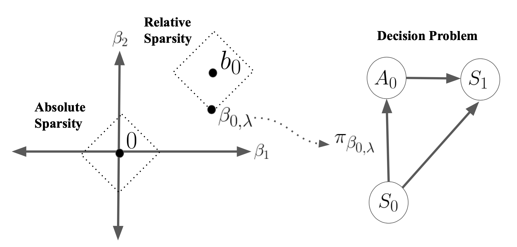
Figure 1: Constraint region of the relative sparsity penalty in the context of a decision problem. We show how the relative sparsity penalty recenters the standard diamond shaped constraints of the $L_{1}$ norm. If we are optimizing over the parameters $\beta=(\beta_{1},\beta_{2})^{T}$ of a policy $\pi_{\beta},$ the relative sparsity constraint region is centered at the parameter of the behavioral policy $b_{0}=(b_{0,1},b_{0,2})^{T},$ whereas the standard lasso constraint region, which gives absolute sparsity, is centered at the zero vector ${\bf 0}=(0,0)^{T}$. Our relative sparsity constraint must be considered in the context of a decision problem, shown to the right. The relative sparsity objective function gives relative interpretability of the policy $\pi_{\beta_{0,\lambda}}$ with respect to the behavioral policy $\pi_{b_{0}},$ which is not guaranteed under the absolute sparsity constraint.

We define an estimator for $J_{0}$ to be

$$J_{n}(\beta,b_{n},\lambda)=V_{n}(\beta,b_{n})-\lambda||\beta-b_{n}||_{1}.$$ (12)

The true parameters of our relatively sparse policy, $\beta_{0,\lambda}=\arg\max_{\beta}J_{0}(\beta,b_{0},\lambda),$ are estimated using $\beta_{n,\lambda}=\arg\max_{\beta}J_{n}(\beta,b_{n},\lambda).$ Note that we ensure that each coefficient is penalized equally by scaling the states as described in Appendix G (assume that any state that we refer to in the simulations, which are in Section 6, and the real data analysis, which is in Section 7, is scaled).

5.2 A problem-specific $\lambda$ selection criterion

The hyperparameter $\lambda$ controls the tradeoff between relative sparsity and value. In the robotics setting of Schulman et al., ⁶⁴ $\lambda$ is often updated iteratively according to Equation (10). In other words, a robot perform a task according to policy 1, updates to policy 2 by defining the behavioral policy as policy 1, performs the task according to policy 2, updates to policy 3 by defining the behavioral policy as policy 2, and so on. In constrast, in healthcare, $\lambda$ must be chosen once, and in a problem-specific manner.

We believe that the appropriate tradeoff between sparsity and value depends on the decision problem. For example, consider blood pressure management in the outpatient, primary care setting. In this setting, we can prescribe a fairly benign blood pressure medication and watch its effect over time. It might be possible to suggest a new policy that changes many of the coefficients with respect to the standard of care, and the providers and patients would still adopt the new policy, because such a policy could lead to large changes in expected reward, or value, with little risk of doing harm to the patient. Now consider the inpatient, intensive care unit setting, where stakes are higher. Blood pressure control might impact the patient’s mortality within minutes. In this setting, a policy must be clearly justifiable relative to established care practices. It might be better if very few of the coefficients diverge from the standard of care, and small increases in expected reward, or value, might be preferable to larger increases that risk causing harm to the patient.

We can obtain policies for these two different scenarios with different settings of $\lambda$, since there will be a tradeoff with respect to expected reward, or value, and relative sparsity. Ideally, one would choose a policy with a difference from behavior that is just sparse enough, but not more sparse, since relative sparsity decreases value. Formally, let us choose a policy with value that is greater than $V^{min}$, which we might define to be the minimal clinically acceptable value. To set $V^{min},$ one might consult guidelines,⁹ or, in a more data-driven fashion, one might set $V^{min}$ to be a value that is some number of standard errors above the value of the behavioral policy. If we determine that, in addition, based on the nature of the decision problem, we would like only approximately $C$ coefficients to differ from behavior (this is perhaps a crude way to measure the “stakes,” but it is at least quantitative), then, if $I(\cdot)$ is an indicator function, we target

$$\lambda_{0}={\max}\left\{\arg\min_{\lambda:{V_{0,\lambda}\geq V^{min}}}|D_{0,\lambda}-C|\right\},$$ (13)

where

$$D_{0,\lambda}=\sum_{k=1}^{K}I\left(|\beta_{0,\lambda,k}-b_{0,k}|>\Delta\right)$$

is the number of coefficients that diverge beyond some tolerance $\Delta\in\mathbb{R}$ from their behavioral counterparts. Hence, we are targeting a sparse policy within the set of policies that have value greater than $V^{min}$. We further take a maximum in Equation (13) to ensure that, of all the policies with $D_{0,\lambda}=C$ and value greater than $V^{min},$ we take the one that has coefficients that are as close as possible to the coefficients of the behavioral policy. Note that one could replace the $\max$ in Equation (13) with a $\min$, which might yield a policy with value that overshoots $V^{min}.$ However, in doing so, we might lose closeness to the behavioral policy. Since we are guaranteed value above $V^{min}$, we recommend instead using a $\min$ in (13) and increasing $V^{min}$ if a policy with higher value is desired. Closeness to behavior, which translates to closeness of the suggested policy coefficients to the behavioral policy coefficients, leads to a more clinically palpable policy, which promotes adoption. If we look at an example of the level sets around $\beta_{0}$ and $b_{0}$, which we show in Figure 2, we can see that, generally,

$$\lambda\leq\lambda^{\prime}\implies V_{0}({\beta_{0,\lambda}})\geq V_{0}({\beta_{0,\lambda^{\prime}}}),$$ (14)

and, hence, we lose some value by taking the maximum in (13), but we gain the maximum closeness to behavior within the set of policies that have value of at least $V^{min}$.

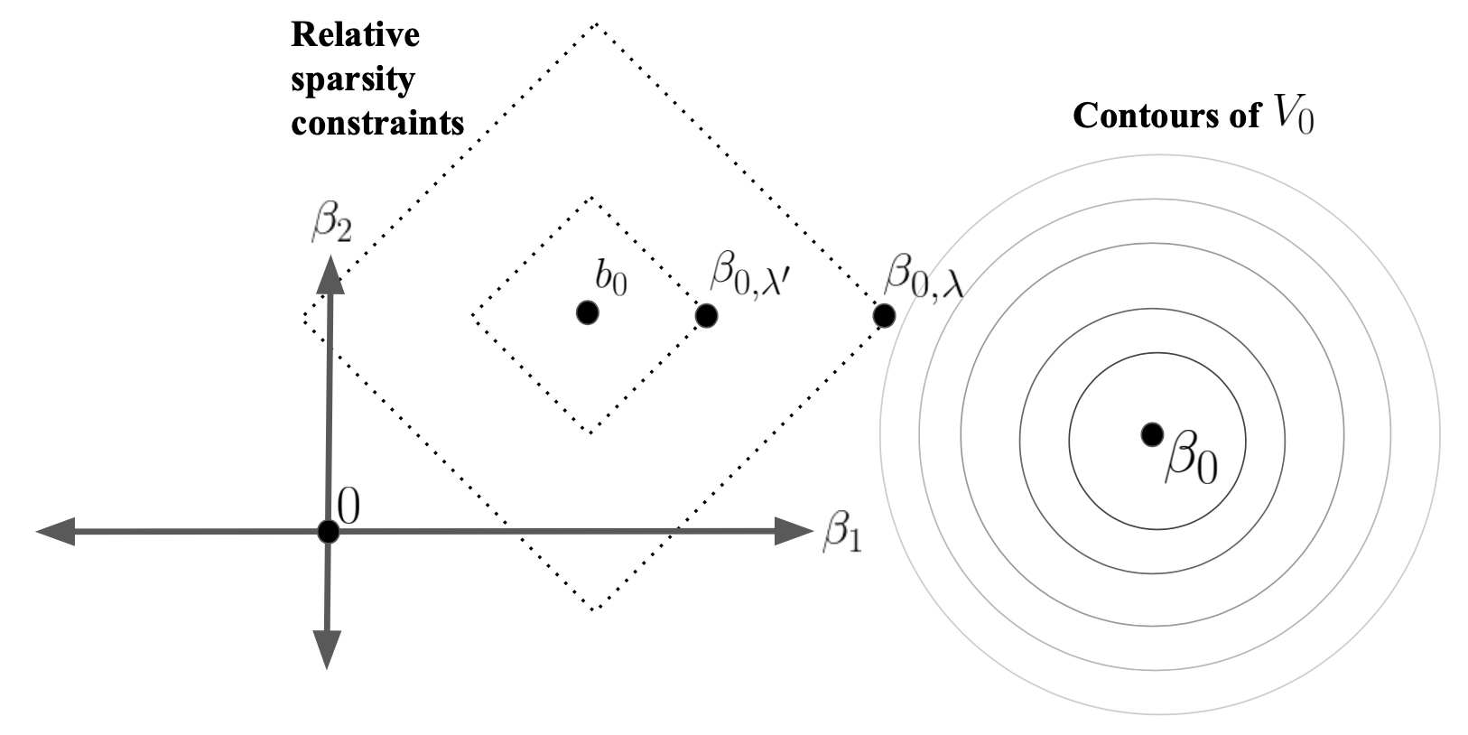
Figure 2: Relationship between $V_{0}({\beta_{\lambda}})$ and $V_{0}({\beta_{\lambda^{\prime}}})$ when $\lambda^{\prime}{>}\lambda$. Consider, as in Figure 1, a bivariate parameter $\beta=(\beta_{1},\beta_{2})^{T},$ which will be chosen to optimize the joint objective, $J_{0}(\beta,b_{0},\lambda),$ in Equation (11). Note that $\beta_{0}=\arg\max_{\beta}V_{0}$ (also, $\beta_{0}=\arg\max_{\beta}J_{0}(\beta,b_{0},0)$) is shown beyond the horizontal axis to indicate that, without loss of generality, $\beta_{0,1}$ happens to be arbitrarily large, and that the contours around $\beta_{0}$ correspond to the contours of $V_{0}(\beta)$, where larger diameter of the contours indicates smaller $V_{0}(\beta)$. Also shown are two possible solutions for $\beta,$ $\beta_{0,\lambda^{\prime}}$ and $\beta_{0,\lambda},$ under relative penalties $\lambda^{\prime}$ and $\lambda$, respectively. Since $\lambda^{\prime}{>}\lambda$, we see that the diamond constraint of the $L_{1}$ norm for the relative sparsity condition is larger for $\lambda$ than for $\lambda^{\prime}$. Since, for a given $\lambda,$ the maximizer of the joint objective, $J_{0},$ must be as close as possible to $\beta_{0}$ but also must fall within the $\lambda$-specific diamond level set, we have that $\beta_{0,\lambda}$ will be closer than $\beta_{0,\lambda^{\prime}}$ to $\beta_{0}$. Since $\pi_{\beta_{0}}$ maximizes $V_{0}$, we have therefore that $V_{0}({\beta_{0,\lambda}})\geq V_{0}({\beta_{0,\lambda^{\prime}}}).$

We acknowledge that the user-defined number of diverging covariates, $C$, might be challenging to set, but we still give practitioners the option; if there is no clear best choice of $C,$ it can be simply set to 1 to target maximum sparsity within the class of policies that achieve value greater than or equal to $V^{min}$. In other words, we are choosing a $\lambda_{0}$ that gives a policy with value above some threshold, $V^{min}$, but that has $D_{0,\lambda_{0}}$ parameters that diverge from behavior, and we want $D_{0,\lambda_{0}}$ to be as close as possible to $C$. Note that $D_{0,\lambda}$ depends on $\lambda$ through $\beta_{0,\lambda}$, which maximizes $J_{0}$ in Equation (11). Note also that $\Delta$ can be set according to the magnitudes of the coefficients; e.g., if the coefficients in the training data are large, we can set $\Delta\approx 1$, whereas if the coefficients are small, we can set $\Delta\approx 0.01$.

We estimate $\lambda_{0}$ with

$$\lambda_{n}={\max}\left\{\arg\min_{\lambda:{V_{n,\lambda}\geq V^{min}}}|D_{n,\lambda}-C|\right\},$$ (15)

where

$$D_{n,\lambda}=\sum_{k=1}^{K}I\left(|\beta_{n,\lambda,k}-b_{n,k}|>\Delta\right)$$

is the number of coefficients that diverge empirically from their behavioral counterparts. Since $D_{n,\lambda_{n}}$ is random, taking values $d_{n,\lambda_{n}},$ we will show tables of its empirical distribution when we perform simulations in Section 6.

To aid in choosing $C$ and $\Delta$, we can perform a visualization of the coefficients in the training set as we vary $\lambda$. As long as only the training data is used, this procedure can be interactive; it may be the case that for some problems we cannot obtain a policy with approximately $C$ coefficients that diverge that also has value above $V^{min}$, in which case we can assess the results in the training data and, in collaboration with the decision makers, perhaps choose a larger target $C$. When $V^{min}$ is large, this may require decision makers to reduce their expectations for sparsity, and vice versa. Having set $V^{min}$ , $C,$ and $\Delta$, we then choose $\lambda$ by minimizing Equation (13). One can then use the test data to estimate the value of the final policy, as we show in Sections 6 and 7. We provide pseudocode in Appendix J.

Corollary 1.

Recall Definition 1, which states that a policy $\pi$ is deterministic if and only if $\pi(a_{0}|s_{0})=1$ or $0$ for all $a_{0},s_{0}.$ Assume the form of the optimal policy follows Equation (1), i.e., $\pi_{\beta_{0}}=\text{expit}(\beta_{0}^{T}s_{0}),$ and that $S_{0,k}<\infty$ for all $k=1,\dots,K$. A policy $\pi_{\beta_{0}}$ is deterministic if and only if one of the entries in its parameter vector $\beta_{0}$ is infinite (or becomes arbitrarily large in magnitude).

Corollary 1, for which we provide a formal proof in Appendix C, follows from the fact that the expit function equals one or zero only when its input is positive or negative infinity (or arbitrarily large). We use the terminology “arbitrarily large in magnitude” because sometimes parameters do not become infinite in magnitude, but approach infinity in magnitude, such that the policy they parameterize is essentially deterministic. Corollary 1 will help us interpret our simulation results and give insight into the behavior of the maximizer of the penalized relative sparsity objective in Equation (11).

5.3 Stochasticity of $\pi_{\beta_{0,\lambda}}$

By Equation (5), which gives an expression for $\pi_{0}=\arg\max_{\pi}V_{0}$ as an indicator function, if $\pi_{\beta_{0}}$ is assumed to be close to $\pi_{0},$ then $\pi_{\beta_{0}}$ is deterministic. Hence, by Corollary 1, $\pi_{\beta_{0}}$ will have some parameters that equal or approach infinity in magnitude. By the following Lemma, however, $\beta_{0,\lambda}=\arg\max_{\beta}J_{0},$ will be finite.

Lemma 1.

For $\lambda>0,$ if we assume Equation (6), Equation (1), and that

$$E(R(S_{0},A_{0},S_{1})|S_{0}=s_{0},A_{0}=a_{0})<\infty$$

for all $s_{0},a_{0},$ then the policy $\pi_{\beta_{0,\lambda}}$ is stochastic. In other words, $|\beta_{0,\lambda,k}|<\infty$ for all $k$ (and $\beta_{0,\lambda,k}$ does not become arbitrarily large in magnitude).

We provide a proof in Appendix D. The finiteness of $\beta_{0,\lambda}$ turns out to play an essential role in the justifiability of $\pi_{\beta_{0,\lambda}}$ with respect to the standard of care, a fact on which we will elaborate in the next section.

5.4 On $L_{1}$, $L_{0}$, and absolute sparsity

In summary, the key objective of our proposed approach is to facilitate the justification and adoption of data-driven treatment strategies, and ultimately enhance our ability to translate decision aids into the clinic. This has motivated us to develop a method that simultaneously controls the (1) closeness, defined as the divergence between the suggested policy probability of treatment, $\pi_{\beta_{n,\lambda_{n}}}(A_{0}=1|S_{0}=s_{0})$, and the behavioral policy probability of treatment, $\pi_{b_{n}}(A_{0}=1|S_{0}=s_{0})$, and (2) sparsity between the coefficients of the behavioral policy and the suggested policy, which, we hypothesize, act in concert to promote the adoption of a new policy in the clinic. This joint closeness and sparsity can be achieved by using an $L_{1}$ norm in the penalty.

Closeness to the standard of care is important, because it is challenging to specify a reward perfectly, and sometimes therefore it is safer to stay close to the standard of care, which is a vetted guideline in many cases. In our method, the $L_{1}$ penalty is important because the $L_{1}$ penalty shrinks, which achieves this closeness to behavior, in addition to selecting, which we need for relative sparsity. That closeness to behavior is important for safety has been explored extensively in other work (see Achiam’s survey ¹ on safe reinforcement learning). Note that, in general, closeness to established guidelines is important in a healthcare setting, because dramatic changes are often not easily accepted or may take a very long time to be adopted.⁴⁰; ⁶¹

Hence, we use an $L_{1}$ penalty not for computational reasons, as is commonly the case when an $L_{1}$ penalty is used to approximate an $L_{0}$ (best subsets) penalty, but instead because the $L_{1}$ penalty, while selecting, which reduces cognitive burden for the end-user, ⁴⁵; ¹²; ⁷⁸ also shrinks the coefficients to behavior. Hence, the $L_{1}$ penalty is, for our motivation, as useful in the low-dimensional case as in the high dimensional case. This desired shrinkage does not occur with an $L_{0}$ penalty. Concretely, define $\beta_{0}^{L_{0}}$ to be a parameter vector in which the reward-relevant parameters are set to their corresponding entries in $\beta_{0}=\arg\max_{\beta}V_{0}$ (also, note that $\beta_{0}=\arg\max_{\beta}J_{0}(\beta,b_{0},0)$), and the reward-irrelevant parameters are set to their corresponding behavioral counterparts in $b_{0}$. This would be the resulting policy if we could use an $L_{0}$ rather than $L_{1}$ penalty, where the $L_{0}$ policy counts the number of non-behavioral coefficients. The $L_{1}$ solution is known to approximate the $L_{0}$ solution, which is useful because the $L_{0}$ problem is NP-Hard. ⁴⁹ The $L_{1}$ solution does not equal the $L_{0}$ solution, because the $L_{1}$ norm shrinks instead of purely selecting coefficients, which is considered a drawback.³ Often, in the literature (e.g., in Tibshirani et al., ⁷²) it is the likelihood that is being penalized, and the selected maximum likelihood estimators are of interest, so it is not desirable to shrink (bias) their estimates.

In our case, however, the fact that the $L_{1}$ penalty shrinks is a benefit. If we could exactly obtain the $L_{0}$ solution, $\beta_{0}^{L_{0}}$, at least one of the selected coefficients would tend toward infinity by Corollary 1. Hence, the coefficients that would be selected in the suggested policy would be arbitrarily larger in magnitude than the unselected coefficients. Hence, the suggested policy would ignore the behavioral covariates, which is not desirable. The property that we call “justifiability” is, in fact, a combination of relative sparsity and also of shrinkage, where the shrinkage must be pronounced enough to allow the behavioral policy coefficients to impact the linear predictor $\beta_{0,\lambda}^{T}s_{0}$ and hence to impact the resulting policy, $\pi_{\beta_{0,\lambda}}$. Hence, the fact that the $L_{1}$ norm shrinks is key to providing a suggested policy that is not dominated by the reward-relevant covariates, as would occur with the $L_{0}$ solution. Thus, the shrinkage that is commonly viewed as a drawback to the $L_{1}$ norm is, in our case, crucial to obtaining a policy with the desired properties.

Define also $J_{0}^{Abs}(\beta,\lambda)$, in contrast to our Equation (11) objective, which is $J_{0}(\beta,b_{0},\lambda)=V_{0}-\lambda||\beta-b_{0}||_{1},$

$$J^{Abs}_{0}(\beta,\lambda)=V_{0}(\beta)-\lambda||\beta||_{1}.$$

Whereas the parameter $\beta_{0}^{L_{0}}$ sets the unselected coefficients to their behavioral counterparts, here the parameter ${\beta^{Abs}_{0}}=\arg\max_{\beta}J_{0}^{Abs}$ sets these same coefficients to zero. However, because the selected coefficients tend in magnitude toward infinity, $(\beta_{0}^{Abs})^{T}s_{0}$ effectively equals $(\beta_{0}^{L_{0}})^{T}s_{0},$ and hence $\pi_{\beta_{0}^{Abs}}$ is indistinguishable from $\pi_{\beta_{0}^{L_{0}}}$. Hence, the shrinkage of the $L_{1}$ penalty is also essential for differentiating the relative sparsity penalty from an absolute sparsity penalty. We show the properties of the relative sparsity objective as it relates to other reinforcement learning methods in Table 1.

	Parametric $\pi_{\beta}$	Max. value	Relative sparsity	Absolute sparsity	Close to behavior	Specify behavior	Specify value or transitions
Proposed (relative sparsity):
$V_{n}(\beta,b)-\lambda L_{1}(\beta,b)$	yes	no	yes	no	yes	yes	no
TRPO64:
$V_{n}(\pi_{\beta},\pi_{b})-\lambda KL(\pi_{\beta},\pi_{b})$	no	no	no	no	yes	yes	no
Absolute relative sparsity:
$V_{n}(\beta,b)-\lambda L_{0}(\beta,b)$	yes	no	yes	no	no	yes	no
Absolute sparsity:
$V_{n}(\beta,b)-\lambda L_{0}(\beta)$	yes	no	no	yes	no	yes	no
Absolute sparsity 77:
$V_{n}(\beta,b)-\lambda L_{1}(\beta)$	yes	no	no	yes	no	yes	no
Unconstrained50:
$V_{n}$	no	yes	no	no	no	yes	no
Q-learning76
	no	yes	no	no	no	no	yes
Sparse Q-learning67
	no	no	no	no	no	no	yes
Model-based:
(standard)70	no	yes	no	no	no	no	yes
Model-based:
($V_{n}-\lambda Likelihood$)18; 16	no	yes	no	no	yes	no	yes

Table 1: The properties of relative sparsity as it relates to other reinforcement learning approaches. “Parametric $\pi_{\beta}$” is whether $\beta$ is parametric. “Max. value” indicates whether the policy is optimal with respect to $V_{0},$ which will never be the case when there is a penalty. “Relative sparsity” indicates whether there will be only a sparse set of coefficients that differ between the behavioral and suggested policy. “Absolute sparsity” indicates whether the policy will have a sparse set of nonzero coefficients, which is equivalent to a relative sparsity to a randomized behavioral policy, which has $b_{0}=(0,\dots,0)$. “Close to behavior” indicates whether the suggested policy probabilities of treatment will be similar to the behavioral policy probabilities of treatment. “Specify behavior” indicates whether we must have a model for the behavioral policy; we consider only the policy search ($\arg\max V_{n}$) objectives for all but the Q-learning and model-based approaches, and hence we consider specification of behavior necessary, because it is necessary for policy search. “Specify value or transitions” indicates whether we must propose models for these aspects of the environment and reward structure, which can be non-trivial, and is required in Q-learning and model-based approaches. For the unconstrained approach, we consider the nonparametric optimizer that achieves maximal value. Note that TRPO can be formulated with a parametric policy, $\pi_{\beta}$, but this is not required, and it is often not the case given that the application area is robotics (the policy might be parametric, but it would be over-parameterized as in Deep Learning).

5.5 Estimation of the behavioral policy

We now describe estimation of the standard of care (behavioral) policy parameters in more detail. The standard of care policy parameters are estimated as $b_{n}$ that maximizes the likelihood, $l_{n}$ (Equation (3)), of the observed data (this can be estimated by using the generalized linear model (GLM) R package). The estimate $b_{n}$ is derived after covariate scaling, so that the covariates for the behavioral policy and for the suggested policy, which are penalized toward one another, pertain to the same data.

Note that $b_{n}$ will be an estimate of $b_{0}$, and the noise in $b_{n}$ will impact the estimation of $\beta_{n,\lambda}$, which is constrained to $b_{n}$. When fitting $\pi_{b_{n}},$ which is a prediction model, we recommend that one follows established guidelines ^{69; 7} for estimating and reporting prediction models. This might include assessment of the behavioral policy model on held out data, as we have included in Figure 7. Note that a calibration curve (computed on held out data) helps us assess the reasonableness of the model specification and the estimation; there is an associated calibration curve shape for a model that is too simple for the true data generating mechanism (an s-shaped curve) and an associated calibration curve shape for an estimation procedure that is overfitting (an s-shaped curve that is reflected over the identity line). ^{74; 25; 52} In our case, since we assume that the behavioral policy is linear in the parameters by Equation (2), we plot a calibration curve to assess whether linearity is too restrictive. In this study, we also reduced noise in estimation of $b_{n}$ by using a penalized estimator,²⁶ where the penalty was chosen by cross validation (this can be done with the CV.GLMNET¹⁷ R package).

6 Simulations

6.1 Scenario

In our simulations, we will investigate a problem inspired by inpatient blood pressure control. In particular, let us consider inpatient hypotension management, which will be the focus of our real data analysis in Section 7. Suppose, as will be the case in the real data analysis, we have determined that healthcare providers take into account $K=9$ covariates when making a decision. Suppose that we have also determined that hypotension management is a high-stakes decision problem, so we fix $V^{min}$ to be the value that is 2 standard errors above the standard of care, and we suppose that the healthcare providers will only adopt a policy that diverges from the standard of care for approximately one covariate. We split the data into a training and test set. We use the training set to better understand how many coefficients will diverge for each $\lambda$, allowing us to assess the feasibility of our requirement on value, $V^{min}$, and the number of diverging coefficients, $C$, and we use the test set to obtain a valid estimate of value, $V_{0}$.

Fix the sample size to be ${n=1000},$ the number of Monte-Carlo repetitions to be $M=500,$ and the states to be $S_{0},S_{1}\in\mathbb{R}^{9}$. Recall from Equation (1) that

$$\pi_{b_{0}}(A_{0}=1|S_{0}=s_{0})=\text{expit}(b_{0}^{T}s_{0}),$$

and set the parameter of the true behavioral policy to be $b_{0}=(-0.01,0.02,0,\dots,0)^{T}$. Hence, although we have a priori suspected that 9 covariates are relevant to the decision problem, the true behavioral actors base their decisions only on the first two covariates.

6.2 Data generation

Draw the initial state $\ S_{0}\sim\text{N}(\mu_{0},\Sigma_{0})$ and draw the action from a Bernoulli distribution,

$$A_{0}|S_{0}\sim\text{Bern}\left(\pi_{b_{0}}(A_{0}=1|S_{0}=s_{0})\right),$$

where $\mu_{0}=(45,\dots,45)^{T}$ and $\Sigma_{0},$ the initial state covariance, is a $K$-dimensional matrix with 300 on its diagonals except for covariance of 100 between $S_{0,1}$ and $S_{0,2}$. We choose this initial state to make the problem directly interpretable in terms of mean arterial pressure (MAP), as in the real data analysis. Draw the final state

$$S_{1}|A_{0},S_{0}\sim\text{N}(S_{0}+\tau{{}^{T}}S_{0}A_{0},\Sigma),$$ (16)

where $\Sigma,$ the transition covariance, is a $K$-dimensional matrix with 300 on its diagonals except for covariance of 200 between $S_{1,1}$ and $S_{1,2}.$ Let the coefficient for the action in Equation (16) be $\tau=(0.1,0.7,0,\dots,0),$ so that only the first and second covariate of the state affect the transition. Note that $\tau$ is also called the “treatment effect.” Set the reward function to be

$$R(S_{0},A_{0},S_{1})=S_{1,2}.$$ (17)

Hence, the transition will depend on two covariates (and hence the reward, which depends on the transition because the transition leads to the final state, will depend on two covariates). If we imagine that the second covariate is blood pressure, then this reward reflects our goal of raising blood pressure, where blood pressure might depend on both the past blood pressure and another covariate, such as heart rate. Since we have made the states in the range of a typical MAP, we will now be able interpret the expected reward as the expected MAP.

The following fact will guide us in ensuring that our simulation results are reasonable. For the reward in our simulations, if the true optimizer of the unpenalized objective is $\beta_{0}=\arg\max_{\beta}V_{0},$ as in Equation (7), then, for $\zeta_{1}$ and/or $\zeta_{2}$ arbitrarily large,

$$\beta_{0}=({\zeta_{1},\zeta_{2}},0,\dots,0).$$ (18)

Equation (18), which is derived in Appendix H, follows from the definition of the reward in Equation (17), an application of Equation (5), and our choice of treatment effect $\tau$. Hence, since $\beta_{0,1}$and $\beta_{0,2}$ tend toward infinity, we expect that $\beta_{0,\lambda,1}$ and $\beta_{0,\lambda,2}$ will have positive signs (note also that $b_{0,2}>0$, so even when $\lambda$ is large, $\beta_{0,\lambda,2}>0$, and the opposite for $b_{0,1}$ and $\beta_{0,\lambda,1}$), but, by Lemma 1, since $L_{1}$ shrinks, neither will be arbitrarily large.

6.3 Results

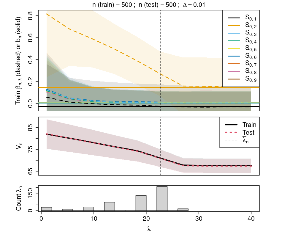
Figure 3: Average coefficients ($\beta_{n,\lambda},b_{n}$) and value ($V_{n}$) in the 500 simulated data sets. In the top panel, the solid, horizontal lines correspond to the coefficients, $b_{n}$, of the behavioral policy, $\pi_{b_{n}}$, and the changing, dotted lines correspond to the coefficients, $\beta_{n,\lambda}$, of the suggested policy, $\pi_{\beta_{n,\lambda}}$. The vertical dotted line, $\bar{\lambda}_{n}$, indicates the choice of $\lambda$ based on Equation (13) when using the average of the coefficients over Monte-Carlo datasets. The bottom panel shows the distribution of the different $\lambda_{n}$ that are selected using Equation (13) over the Monte-Carlo datasets. Note that $\Delta$ is the threshold for considering a coefficient equal to its behavioral counterpart. Note that we do not start the $\lambda$ grid at 0, since the unconstrained version is difficult to optimize, and the coefficient magnitudes for the unconstrained version are very large, so the range of the y-axis becomes large as well, making it difficult to visualize the changes in coefficients within the desired $\lambda$ range.

We see in Figure 3, which shows the average coefficients over 500 datasets, that, as $\lambda$ increases along the horizontal axis, the relative sparsity penalty shrinks reward-irrelevant coefficients to their behavioral counterparts. We show confidence intervals for the coefficients $\beta_{n,\lambda}$ using a Monte-Carlo standard error estimate, as described in Appendix F. For the confidence intervals around $V_{n}$, we use the estimator described in Appendix E and take an average of these confidence intervals over datasets. The coefficients in the top panel are the averages over datasets, and the $\bar{\lambda}_{n}$ selection in the middle panel of Figure 3 is made by optimizing the criterion in Equation (13) for these average coefficients (we do this once with the averages, to show how one selection would appear based on the top panel, and we also do this for each dataset, to show the distribution of selections). The $\bar{\lambda}_{n}$ selection on the average coefficients occurs when one coefficient is non-behavioral, since $C=1.$ Since this is a simulation, and we generate multiple datasets, we also employ our $\lambda$ selection criterion in Equation (13) for each of the individual Monte-Carlo datasets, giving $M$ selections of $\lambda_{n}$, and we show the distribution of $\lambda_{n}$ in the bottom panel of Figure 3. Based on the $\lambda_{n}$ that is selected in each dataset, we have corresponding covariates that are selected (i.e., their coefficients are not set to their behavioral counterparts).

We show the distribution over simulated datasets of the value function $V_{n},$ the mean estimated probability of treatment (and its closeness to behavior), and the degree of relative sparsity. We show this for the true optimal policy, the unconstrained optimization of $V_{n}$, the constrained optimization of $J_{n}$ (with selected $\lambda_{n}$), and the behavioral policy, in Figure 4. We see that, as expected, the value without a penalty is higher on average, because we lose some value by constraining toward behavior, but we gain proximity to behavior and relative sparsity in doing so. Note still that, over Monte-Carlo datasets, the distribution of which is shown in Figure 4, the observed/ behavioral policy has expected blood pressure of $V_{n}=67.60$ and that the suggested policy has expected blood pressure of $V_{n}=74.12$, where the latter is at least two standard errors above the observed policy. Note that other methods that find an optimal policy, but do not require modeling of the behavioral policy, would give the same solution as the top row of Figure 4, and they do not allow us to obtain relative sparsity or closeness to behavior, since neither the behavioral nor the suggested policy is modeled directly, and any closeness to behavior precludes optimality. Methods like TRPO (Equation 10) allow us to obtain closeness to behavior, but not relative sparsity, since the KL divergence penalty does not impose sparsity (for more discussion, see Table 1).

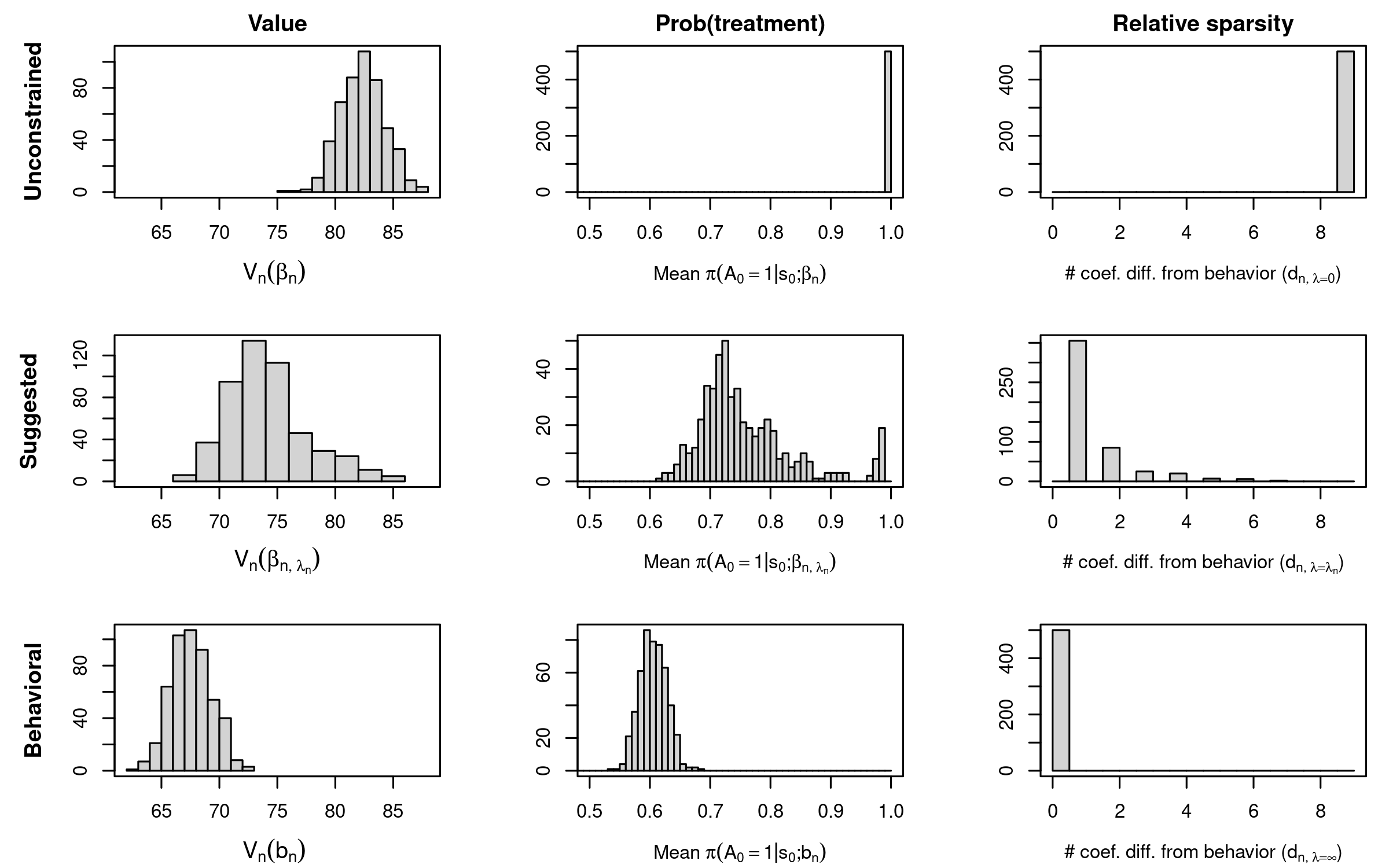
Figure 4: Empirical distributions of value, probability of treatment, and relative sparsity for data policies over simulated datasets. We show the distribution over simulated datasets of the value, mean estimated probability of assigning treatment (and its proximity to behavior), and relative sparsity. We show these plots for unconstrained optimization ($\beta_{n}=\arg\max_{\beta}V_{n}$ , which would be the result of any reinforcement learning method that just finds the optimal policy, and allows neither closeness to behavior nor relative sparsity); for the suggested policy ($\beta_{n,\lambda_{n}},$ where $\beta_{n,\lambda}=\arg\max_{\beta}J_{n}$); and for the behavioral policy, $b_{n}=\arg\max l_{n}$, where $V_{n},J_{n},$ and $l_{n}$ are value, penalized value, and log likelihood, respectively. Note that the suggested policy provides value, closeness to behavior, and relative sparsity, all of which facilitate adoption of the suggested policy into the clinic.

,

	$S_{0,1}$	$S_{0,2}$	$S_{0,3}$	$S_{0,4}$	$S_{0,5}$	$S_{0,6}$	$S_{0,7}$	$S_{0,8}$	$S_{0,9}$
$\hat{P}(selected)$	0.27	0.97	0.12	0.10	0.12	0.10	0.10	0.10	0.11

Table 2: Selection proportion for each covariate over 500 simulated datasets. Note that only $S_{0,2}$ and, to a lesser extent, $S_{0,1},$ are truly relevant to the reward, and that there is some correlation between $S_{0,1}$ and $S_{0,2}$.

To better characterize the relative sparsity that we observe in the policies estimated on the simulated datasets, we include the distribution of $D_{n,\lambda_{n}},$ the number of selected coefficients over Monte-Carlo datasets, as defined by Equation (13), in Figure 4. We see that $D_{n,\lambda_{n}}$, the number of diverging parameters under the selected $\lambda_{n},$ matches our target of $C=1$ more than half of the time, and that we approximately achieve our goal of $C=1$ in all cases. Sometimes we also select $D_{n,\lambda_{n}}=2,$ due to the correlation between $S_{0,1}$ and $S_{0,2}.$ We report the covariate selection proportions in Table 2, where we see that the most reward-relevant covariate, $S_{0,2},$ is most often selected (along with sometimes the covariate $S_{0,1}$, which is correlated with $S_{0,2}$ and more faintly related to the reward. The other covariates are selected less often).

7 Real data analysis

7.1 Research objective

There is variability in vasopressor administration for hypotensive patients in the intensive care unit (ICU), and trials on vasopressors have been inconclusive. ³⁹; ¹⁰; ⁶³ Vasopressor usage is therefore an interesting potential target for medical decision models. Vasopressor use in the inpatient setting can impact a patient greatly, and the onset of action is often in minutes. Vasopressors can stabilize blood pressure, but they have a variety of adverse effects. Secondary to excessive vasoconstriction, vasopressors can cause organ ischemia and infarction, hyperglycemia, hyperlactatemia, tachycardia, and tachyarrhythmias. ⁶³ Whether to prescribe vasopressors is a subtle and high stakes decision. To change behavior with respect to vasopressor usage, therefore, any divergence from the established care guidelines should be clear and justifiable. Let us therefore try to obtain a policy that has value at least 2 standard errors above the behavioral policy, but that diverges from behavior with respect to only 1 or 2 covariates.

7.2 Dataset and cohort selection

We consider the MIMIC III dataset, ³²; ³¹; ²⁰ which is a freely available, observational electronic health record dataset from the Beth Israel Deaconess Medical Center. We briefly describe cohort selection. We consider only the medical ICU (i.e., we do not consider the surgical or trauma ICUs). If a patient has been hospitalized multiple times, we take the first hospitalization, and if a patient is admitted to the medical ICU multiple times within one hospital stay, we take the first medical ICU stay. In our decision problem, which we will describe in detail in Section 7.3, we will analyze a time window that begins at hypotension onset and lasts 30 minutes. We excluded the 7 out of $n=4,715$ patients who left the ICU before those 30 minutes had elapsed.

7.3 Decision problem

We amend code from Futoma et al. ¹⁸ to obtain a decision problem that begins approximately at the onset of hypotension. Hypotension is assessed according to mean arterial pressure (MAP), a weighted average of diastolic and systolic blood pressures, where the weights reflect the amount of time in diastole and systole; MAP is also the product of cardiac output and total peripheral vascular resistance. We define time zero to be approximately at the first MAP$<60$, which is a threshold for hypotension. ⁷⁹; ³⁹ After 15 minutes, we construct $S_{0},$ which contains a summary of all of the covariates at this time point. We found it was better to let $S_{0}$ be a summary of the first 15 minutes instead of the observed MAP$<$60 itself, because one MAP$<60$ may be influenced by random fluctuations, whereas if MAP$<60$ at time zero and is still $<60$ after 15 minutes, then it is likely that the patient is experiencing a sustained hypotensive episode. We use the set of covariates from Futoma et al., ¹⁸ which includes MAP, heart rate (HR), urine output, lactate, Glasgow coma score (GCS), serum creatinine, fraction of inspired oxygen (FiO2), total bilirubin, and platelet count. These covariates would all be of interest when deciding whether to administer vasopressors. For MAP, if there was more than one measurement within a time interval, we used the most recent, assuming the most recent measurement would be most relevant as a reward and when deciding whether to administer vasopressors in the next time step. These covariates, taken as a vector, define the state. The action $A_{0},$ based on $S_{0}$, is whether to administer vasopressors from time 15 minutes to time 30 minutes. The final state, $S_{1},$ contains a summary of MAP and all other covariates at 30 minutes.

The vasopressor units are total micrograms of medication given each hour per kilogram of body weight. In particular, as in Futoma et al., ¹⁸ we consider Dopamine, Epinephrine, Norepinephrine, Vasopressin, and Phenylephrine. The various doses and brands of vasopressors are converted based on the code in Futoma et al. ¹⁸ to a Norepinephrine equivalent using the method in Komorowski et al. ³⁸ Intravenous Norepinephrine has a half life of approximately 2.4 minutes. ⁶⁶ Hence, we consider the MAP at 30 minutes to depend only on the vasopressors administered from 15-30 minutes, and not on those administered from 0-15 minutes. Since we analyze intensive-care-unit data, most patients are started on vasopressors before the 15 minute time point, in which case our decision becomes whether to continue or to stop the medication. We finally define a reward that reflects the short term goal of increasing MAP in the setting of severe hypotension. In our real data analysis, we took MAP to be the first covariate in the state, so we define the reward to be $R(S_{0},A_{0},S_{1})=S_{1,1}.$ Vasopressors should increase this reward.

As an example of a trajectory, one patient was found to have MAP=58, which indicated hypotension. Vasopressor infusion was initiated within minutes. From 0-15 minutes, as the patient received the vasopressor infusion, their MAP changed from 58 to 48. Hence, since we take MAP to be the first covariate, we had MAP=48 as $S_{0,1}$. From 15-30 minutes, the vasopressor infusion was maintained, so $A_{0}=1$. Finally, at 30 minutes, MAP=53, so $S_{1,1}=53$. Hence, this patient had trajectory $(S_{0,1}=48,A_{0}=1,S_{1,1}=53)$ and $R(S_{0},A_{0},S_{1})=53$ (in practice, the state covariates are scaled, as described in Section 5.1 and Appendix G, but this is essentially the trajectory).

The measurements that contribute to the covariates are provided in extensive tables that are part of the MIMIC-III database (e.g., one of the tables has roughly 330 million rows), which were processed using bash scripts from Futoma et al. ¹⁸ As in Futoma et al., ¹⁸ extreme, non-physiologically feasible values of covariates were floored or capped, missing static covariates were imputed by the median, and time dependent covariates were imputed by last observation carry forward.

7.4 Results

We first evaluate the specification of the model for the behavioral policy in Equation (2), which is integral to inverse probability weighting in Equation (8) and also to the penalty in Equation (12). For this, we show a calibration curve (Figure 7 of Section I). We see high concordance between the observed and estimated probabilities, and therefore we conclude that our model for the behavioral policy, Equation (2), is a reasonable model, and that we can then proceed with optimizing Equation (12) for the proposed method. Since we only have one real dataset, unlike in simulations, we split the data into single train and test sets, but we repeat this split 100 times and average the results. We recommend that this resampling be done if the objective function is not otherwise⁷¹ stabilized. We show the coefficient paths as a function of $\lambda$ in Figure 5. We see that the coefficient for MAP withstands the relative sparsity penalty, requiring a large $\lambda$ to finally reach its behavioral counterpart, whereas coefficients for variables like platelet count quickly approach their behavioral counterparts, causing virtually no change in value. To best assess which coefficients withstand the push to behavior, and how this impacts the value, $V_{n}$, it is vital to perform some type of repeated sampling, as we have done here, because the individual test train splits can be noisy. One can also stabilize $V_{n}$ in other ways,⁷¹ which might be less computationally intensive.

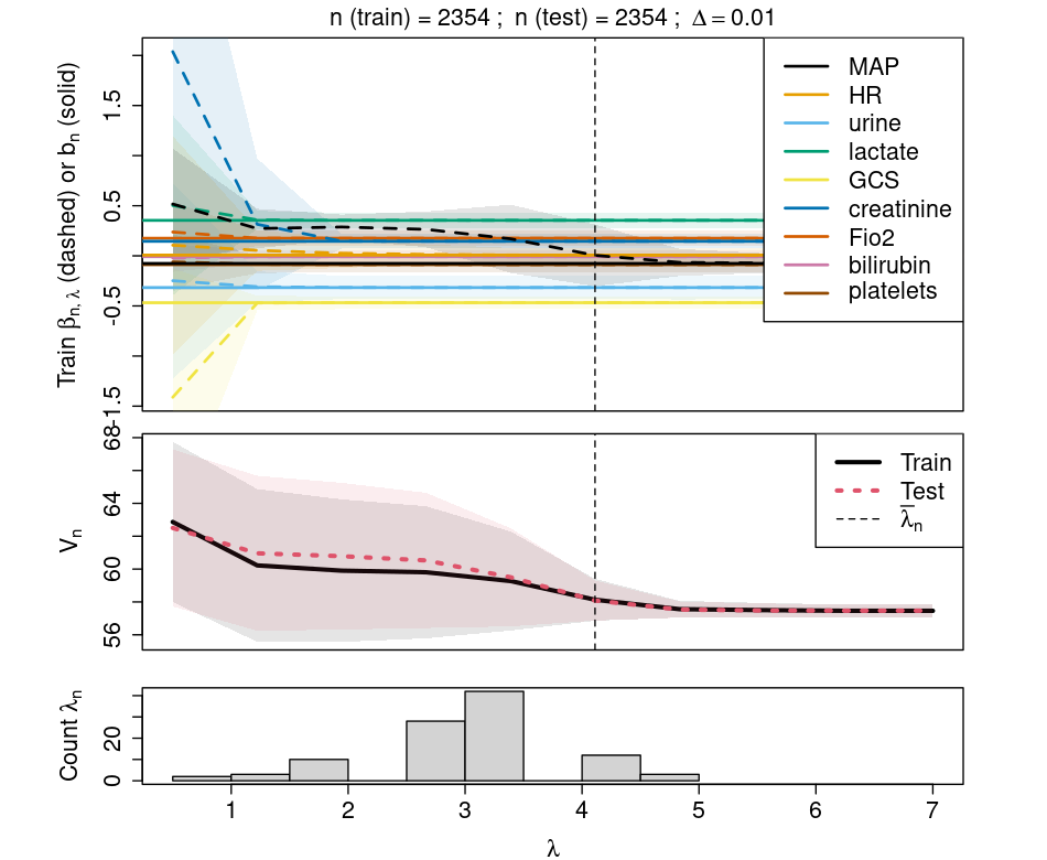
Figure 5: Coefficients ($\beta_{n,\lambda},b_{n}$) and value ($V_{n}$) in the real data set. In the top panel, the solid, horizontal lines correspond to the coefficients, $b_{n}$, of the behavioral policy, $\pi_{b_{n}}$, and the changing, dotted lines correspond to the coefficients, $\beta_{n,\lambda}$, of the suggested policy, $\pi_{\beta_{n,\lambda}}$. The dotted vertical line in the bottom panel indicates a choice of $\lambda$ based on maximizing Equation (13) in the training data. Note that $\Delta$ is the threshold for considering a coefficient equal to behavior and was chosen based on visual inspection of the top panel. We average over 100 resamples of the real data; we show the distribution of the selected $\lambda_{n}$ over resamples, but the final selection of the penalty weight, $\bar{\lambda}_{n}$, was based on the average coefficients and value over resamples. Note that we do not start the $\lambda$ grid at 0, since the unconstrained version is difficult to optimize, and the coefficient magnitudes for the unconstrained version are very large, so the range of the y-axis becomes large as well, making it difficult to visualize the changes in coefficients within the desired $\lambda$ range.Note that these confidence intervals for the coefficients, which serve just as a visualization of uncertainty, have different meaning under Monte-Carlo resampling than under repeated sampling of the real data (for more details on the resampling-based construction of confidence intervals for the coefficients, see Appendix F).

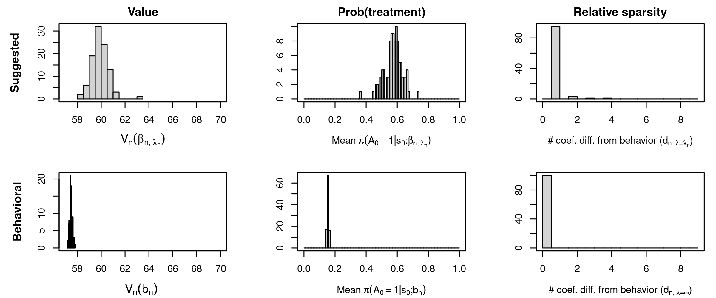
Figure 6: Empirical distributions of value, mean probability of treatment, and relative sparsity for data policies over resamples of the real data. We show the distribution over resampled datasets of the value, mean estimated probability of assigning treatment (and its proximity to behavior), and relative sparsity. We show these plots for the suggested policy ($\beta_{n,\lambda_{n}},$ where $\beta_{n,\lambda}=\arg\max_{\beta}J_{n}$); and for the behavioral policy, $b_{n}=\arg\max l_{n}$, where $V_{n},J_{n},$ and $l_{n}$ are value, penalized value, and log likelihood, respectively. Note that the suggested policy provides value, closeness to behavior, and relative sparsity, all of which facilitate adoption of the suggested policy into the clinic.

Here, we determined that for the criterion in Equation (13), given value, $V_{n}$, that is at least as great as $V^{min}$, $C=1$ diverging covariates would be acceptable. Note that $\Delta$ is the threshold for considering a coefficient equal to behavior and was chosen based on visual inspection of the top panel. We ultimately see that we are able to illustrate the behavior of the relative sparsity penalty with real data, and that we obtain a policy that is sparse relative to the behavioral policy while on average increasing value, $V_{n}$. In the real data, over resampled datasets, the distributions of which are shown in Figure 6, the average final MAP when following the standard of care is 57.46, while the average final MAP when following the suggested policy is 59.89, an increase of more than two standard errors (and 60 is the limit at which the vital organs are adequately perfused ⁹).

In particular, to justify this suggested policy to providers and patients, we only need to discuss MAP, because the parameters for all of the other covariates align with the existing standard of care. Recall that every patient in the cohort was determined to be hypotensive, and that we observe them for 15 minutes to obtain their initial MAP (which is used to determine whether to treat), and then we observe them for another 15 minutes to obtain their final MAP (the reward). Note that the behavioral coefficient on the initial MAP is negative. In the behavioral policy, the providers prefer to treat patients with lower initial MAP more than patients with higher initial MAP; this makes intuitive sense, since blood pressure should be treated when it is low. In the unconstrained, reward-maximizing policy (or the “optimal” policy), the coefficient on initial MAP is positive. The optimal policy would require that all patients be treated, and that patients with higher initial MAP be treated more than patients with lower MAP (within the cohort of hypotensive patients). The suggested policy, with a coefficient for MAP that is near zero, is somewhere in the middle; it tends to treat patients with higher initial MAP along with patients with lower initial MAP, and this increases the average reward. More discussion on the MAP coefficient as it jointly relates to residual confounding, the specified reward, and the decision problem, is provided in the next section.

8 Discussion

8.1 Summary

We show how the relative sparsity penalty can be used to obtain a policy that is easy to explain in the context of the current standard of care, and therefore readily justifiable. We contrast our work with existing KL-based behavior constraints,⁶⁴ which have been primarily focused on applications in robotics, and in which the difference between the suggested and behavioral policy is a black box. Our methodology, which makes the difference between the suggested and behavioral policy sparse, and therefore more interpretable, has strong practical implications for the adoption (and interrogation) of data-driven decision aids in a healthcare setting.

8.2 Limitations and future work

We first discuss some real data analysis limitations. We emphasize that any policy derived with our method should be reviewed by the medical care team, and we hope that our method, in its interpretability, facilitates this type of review.

We discuss the implications and plausibility of the assumptions needed for causal identification. A major assumption is that we have measured all confounders. Our list of covariates (given in Section 7.3), which match those in Futoma et al., ¹⁸ appears to be quite comprehensive for this problem, but it is also important to recognize that the no unmeasured confounders assumption cannot be tested empirically. We note that the suggested policy has a positive, though near zero, coefficient on MAP, whereas the behavioral policy, or standard of care, has a negative coefficient on MAP. This may be because of residual confounding. There are different etiologies of hypotension (e.g., sepsis and hemorrhage ⁶⁸), which are associated with different mechanisms by which the body becomes hypotensive (e.g., different effects on vasopressor-binding adrenergic receptors ¹⁹; ⁸; ⁶⁸), which might in turn alter the way the body responds to vasopressors. It may be the case that one subgroup, e.g. with hypotension due to sepsis, responds less strongly to vasopressors and has a lower baseline MAP than another subgroup, e.g. with hypotension due to hemorrhage. To maximize the average reward, or the average final blood pressure, over these two subgroups of patients, it makes sense to preferentially treat the subgroup of patients who have stronger responses to vasopressors. The standard of care, however, might be more likely to give vasopressors to the subgroup experiencing sepsis than to the subgroup experiencing hemorrhage (generally, vasopressors and fluids are the first line treatment for sepsis, whereas there is more controversy about using vasopressors for hemorrhage ²²; ⁶). In such a case, the signs on the MAP coefficient for the behavioral and reward-maximizing policy, to which the suggested policy is drawn, may be different. Therefore, the subgroup to which patients belong may be an unmeasured confounder. These subgroups might be quite complex and interact with patient characteristics.⁴⁴ Although the covariates in Futoma et al.,¹⁸ which we use in our real data analysis, might fluctuate somewhat according to subgroup, a covariate that identifies these subgroups explicitly is not included. This may be because of the difficulty in establishing such subgroups. Sometimes, diagnoses such as “sepsis” are assigned at the end of the hospitalization (which makes it difficult to establish the time of onset), and such assignments, which are often generated for claims, can be of poor quality.⁶² It would be interesting to possibly use microbiology results to, e.g., determine sepsis status in future work. The MIMIC dataset has many additional covariates, and considering the high-dimensional case might also be a direction of future work.

The specified reward, which is the final MAP in our case, might also be partially responsible for the positive coefficient for MAP in the reward-maximizing policy, to which the suggested policy is drawn. In particular, the specified reward may be over simplified. Although it is sensible to increase MAP, a reward that is based only on increasing MAP may be overly simplistic because it leaves out other aspects that might also be important. This specified reward could be improved by taking into account mortality and morbidity.³⁹ When taking into account mortality and morbidity, the reward-maximizing policy might be more discerning with respect to the coefficient on MAP. A more indirect way to take into account mortality and morbidity using the proposed method would be to change the weight that we place on the specified reward by setting a smaller minimum value cutoff for the suggested policy, or a smaller $V^{min}$ in (13). By sacrificing some value, this allow us to choose a tuning parameter that yields a suggested policy that is closer to the standard of care. The standard of care optimizes its own reward, which likely takes into account mortality and morbidity, and, therefore, by choosing a policy that is close to the standard of care, we can do the same.

In general, the proposed method provides transparency about the coefficients that change when moving from the behavioral to the suggested policy. This generates useful discussion about the coefficients. If the difference between a coefficient in the suggested policy and the standard of care is not clinically palpable, action must be taken before implementation of the policy into the clinic. First, if it is suspected that confounders are unmeasured, these confounders should be collected if at all possible. There will sometimes be evidence of this, because the standard of care coefficients might be unexpected, or, upon consult with a provider, we might find that they take into account some outcome-influencing variables that we had not collected. Second, if it is suspected that the reward function is overly simplistic, then one can discuss lowering the minimum value, $V^{min}$ in (13), in order to move toward the standard of care. Third, one might also re-evaluate the decision problem. In our case, for example, the problem is somewhat simplified; we have discretized time, and we have not taken into account mortality and morbidity in the reward. This has allowed us to avoid methodology needed for survival analysis⁵ and continuous time, ³⁰ which could be the subject of future work. Note also that reward function learning is an active area of research. ⁵¹; ⁵⁹

The high concordance between observed and estimated probabilities seen in the calibration curve further supports the functional form posited for the behavioral policy in Equation (2), which we also consider to be a causal assumption, because the form of the behavioral policy plays such an important role in inverse probability weighting. For cases when Equation (2) does not hold, which would be detectable by a calibration curve, one could improve any issues with model misspecification by using basis expansions of the states. This then allows us to fit a complex behavioral function that is still linear in the parameters, but not in the covariates (e.g., consider $\beta_{1}HR$ + $\beta_{2}MAP$ vs. $\beta_{1}HR$ + $\beta_{2}HR^{2}+\beta_{3}MAP+\beta_{4}MAP^{2}$). We could then map the bases to their respective covariates, and describe which covariates change from behavior accordingly. Another direction for future work would be to consider decoupling, ²⁷ in which case we could make the behavioral policy in the value nonparametric and make the behavioral policy in the penalty parameteric (possibly with basis expansions). Such an addition might complicate convergence of the inverse probability weighted estimator, which is known to be sensitive to nonparametric nuisance parameters, especially in the high-dimensional case, but this may be acceptable with a large enough sample. This is a consequence of slower convergence of the nonparametric estimator.¹⁴ Note that although there are other methods that allow one to sidestep the difficulty in specifying the behavioral policy altogether, these methods do not model the suggested policy directly, and therefore do not allow us to obtain relative sparsity between the coefficients of the behavioral policy and the suggested policy (for more discussion, see Section 5.4 and Table 1). As in any modeling, overfitting is always a risk, for both the behavioral and suggested policy. For the behavioral policy, we describe our method to prevent overfitting in Section 5.5. We believe that the overfitting issue for the suggested policy is mitigated by the parametric nature of the models and by the penalty toward behavior. We believe that evidence for the suggested policy not overfitting is that the out of sample (test) value function (in Figures 3 and 5) corresponding to suggested policy is a nondecreasing function (and matches the training value function). Specifically, if the suggested policy estimates were affected by overfitting, the resulting test value function might increase and then decrease (or be nonsmooth with several local minima and maxima).

In terms of causal assumptions, we also assume positivity, or that in the behavioral policy/standard of care any action is possible given any state, which can be tested empirically, and we did so in the preliminary data analysis that accompanied this work. Other causal assumptions include the stable unit treatment value assumption (SUTVA) and consistency of the states as potential outcomes of the actions, both of which are generally reasonable, since we observe the blood pressure under a certain treatment, and one patient’s treatment does not influence another patient’s blood pressure. We have included some additional references^{36; 46; 23; 80; 35} on causal identification in our setting. We emphasize that even with careful consideration of the plausibility of the causal assumptions, as we have attempted here, it is important to conduct trials to evaluate any clinical decision aids before translation to routine care.

In conclusion, we present a method to obtain policies that are easy to explain in the context of the standard of care. We believe that using statistical methods to help solve decision problems in healthcare will be an iterative process involving collaboration among data analysts, healthcare providers, and patients. We hope that the proposed methodology can help us better explain and justify data-driven policies to healthcare providers and patients, facilitating the adoption of these policies and invigorating the discussion.

Supporting information

Research code can be found at https://github.com/samuelweisenthal/relative_sparsity. Code from Futoma et al. ¹⁸ can be found at https://github.com/dtak/POPCORN-POMDP.

Data availability statement

The MIMIC ³³ dataset that supports the findings of this study is openly available at PhysioNet (doi: 10.13026/C2XW26) and can be found online at https://physionet.org/content/mimiciii/1.4/.

Appendix A Derivation of importance sampling estimand

We show a derivation of Equation (8). Note,

$$V_{0}(\beta) =E_{\beta}[R(S_{0},A_{0},S_{1})]$$

$$=E_{b_{0}}\left\{\frac{P_{\beta}(S_{0},A_{0},S_{1})}{P_{0}(S_{0},A_{0},S_{1})}R(S_{0},A_{0},S_{1})\right\}$$

$$=E_{b_{0}}\left\{\frac{P_{0}(S_{0})\pi_{\beta}(A_{0}|S_{0})P_{0}(S_{1}|A_{0},S_{0})}{P_{0}(S_{0})\pi_{b_{0}}(A_{0}|S_{0})P_{0}(S_{1}|A_{0},S_{0})}R(S_{0},A_{0},S_{1})\right\}$$

$$=E_{b_{0}}\left\{\frac{\pi_{\beta}(A_{0}|S_{0})}{\pi_{b_{0}}(A_{0}|S_{0})}R(S_{0},A_{0},S_{1})\right\}.$$

Appendix B Proof that the maximizer of unpenalized value is an indicator

Although Equation (5) is a known result,⁵⁶; ⁴; ³⁴ we prove it here, for completeness, in our notation and for our problem setting. Write

$$V_{0}(\pi) =E_{\pi}\left(R(S_{0},A_{0},S_{1})\right)$$

$$=E_{\pi}\left(E(R(S_{0},A_{0},S_{1})|S_{0},A_{0})\right)$$

$$=\int_{s_{0}}E\left(R|S_{0}=s_{0},A_{0}=1\right)\pi(A_{0}=1|s_{0})p(s_{0})d{s_{0}}$$

$$+\int_{s_{0}}E\left(R|S_{0}=s_{0},A_{0}=0\right)\pi(A_{0}=0|s_{0})p(s_{0})d{s_{0}}$$

$$=\int_{s_{0}}E\left(R|S_{0}=s_{0},A_{0}=1\right)\pi(A_{0}=1|s_{0})p(s_{0})d{s_{0}}$$

$$+\int_{s_{0}}E\left(R|S_{0}=s_{0},A_{0}=0\right)(1-\pi(A_{0}=1|s_{0}))p(s_{0})d{s_{0}}$$

$$=\int_{s_{0}}\left(E\left(R|S_{0}=s_{0},A_{0}=1\right)-E\left(R|S_{0}=s_{0},A_{0}=0\right)\right)\pi(A_{0}=1|s_{0})p(s_{0})d{s_{0}}$$

$$+\int_{s_{0}}E\left(R|S_{0}=s_{0},A_{0}=0\right)p(s_{0})d{s_{0}}$$

$$=I+II,$$

where

$$I=\int_{s_{0}}\left(E(R|S_{0}=s_{0},A_{0}=1)-E(R|S_{0}=s_{0},A_{0}=0)\right)\pi(A_{0}=1|s_{0})p(s_{0})d{s_{0}}$$

and the second term, $(II),$ does not depend on $\pi,$ so we can ignore it when we consider the maximization of ${V_{0}}.$ Suppose

$$E(R|S_{0}=s_{0},A_{0}=1)-E(R|S_{0}=s_{0},A_{0}=0)>0.$$

If so, since $\pi(A_{0}=1|s_{0})\leq 1,$ then

$$\int_{s_{0}}\left(E(R|S_{0}=s_{0},A_{0}=1)-E(R|S_{0}=s_{0},A_{0}=0)\right)\pi(A_{0}=1|s_{0})p(s_{0})d{s_{0}}$$

$$\leq\int_{s_{0}}\left(E(R|S_{0}=s_{0},A_{0}=1)-E(R|S_{0}=s_{0},A_{0}=0)\right)p(s_{0})d{s_{0}}.$$

Hence,

$$\pi_{0}(A_{0}=1|s_{0})=I(E(R|S_{0}=s_{0},A_{0}=1)-E(R|S_{0}=s_{0},A_{0}=0)>0).$$

Appendix C Proof of Determinism Corollary

We prove Corollary 1. Recall, by Definition 1, that if a policy $\pi$ is deterministic, then $\pi(A_{0}=1|S_{0}=s_{0})=1$ or $0.$ Recall that by Equation (1),

$$\pi_{\beta_{0}}(A_{0}=1|S_{0}=s_{0})=\text{expit}(\beta_{0}^{T}s_{0}).$$

Now, if $\text{logit}(p)=1/(1-p),$ then

$$\text{expit}(\beta_{0}^{T}s_{0})=1\iff\text{logit}(\text{expit}(\beta_{0}^{T}s_{0}))=\text{logit}(1)\iff\beta_{0}^{T}s_{0}=\infty\iff\exists\ k\ \text{ s.t.}\ |\beta_{0,k}|=\infty,$$

since $s_{0,k}<\infty,\ \forall k$ and $\text{logit}(p)\rightarrow\infty$ as $p\rightarrow 1$.

We say however that the entries of $\beta_{0}$ tend in magnitude toward infinity rather than “equal” infinity in magnitude because, for some rewards, setting entries of $\beta_{0}$ equal in magnitude to infinity can lead to an undefined linear predictor, $\beta_{0}^{T}s_{0}$. For example, let $S_{0}\in\mathbb{R}^{2}$ and consider the maximization of $V_{0}=E_{\beta}R$ with $R(S_{0},A_{0},S_{1})=(S_{0,1}-2S_{0,2})A_{0}$. Note that

$$E_{\beta}R(S_{0},A_{0},S_{1}) =E_{\beta}[(S_{0,1}-2S_{0,2})A_{0}]$$

$$=E_{\beta}[E[(S_{0,1}-2S_{0,2})A_{0}|S_{0}]]$$

$$=E_{\beta}[(S_{0,1}-2S_{0,2})E[A_{0}|S_{0}]]$$

$$=E_{\beta}[(S_{0,1}-2S_{0,2})\text{expit}(\beta^{T}S_{0})]$$

$$=E_{\beta}[(S_{0,1}-2S_{0,2})\pi_{\beta}(A_{0}=1|S_{0})].$$

The last line is maximized by

$$\pi_{\beta_{0}}=I(S_{0,1}-2S_{0,2}>0).$$ (19)

Since we have a policy $\pi_{\beta_{0}}=\text{expit}(\beta_{0,1}S_{0,1}+\beta_{0,2}S_{0,2}),$ we can approximate this indicator by setting $\beta_{0,1}$ arbitrarily large but finite, and $\beta_{0,2}=-2\beta_{0,1},$ so that

$$\pi_{\beta_{0}}=\text{expit}(\beta_{0,1}S_{0,1}-2\beta_{0,1}S_{0,2})=\text{expit}(\beta_{0,1}(S_{0,1}-2S_{0,2})),$$

which approximates the indicator in Equation (19) as $\beta_{0,1}$ becomes large in magnitude. However, if we set $\beta_{0,1}=\infty,$ we get $\beta_{0,2}=-2\infty=\infty,$ and

$$\pi_{\beta_{0}}(A_{0}=1|S_{0}=s_{0})=\text{expit}(\infty S_{0,1}-\infty S_{0,2}),$$

which is undefined.

More generally, the standard rules of arithmetic must hold for the entries of $\beta_{0}$, which is not the case when one or more entries of $\beta_{0}$ is infinite in magnitude. Hence, it appears that for some rewards, a linear model might simply not be expressive enough; we can never have $\pi_{0}$ be equaled by $\pi_{\beta_{0}}$, since $\pi_{0}$ is a deterministic indicator function and $\pi_{\beta_{0}}$ that maximizes the expected reward cannot have coefficients that are infinite in magnitude, and therefore cannot be deterministic. In practice, an expit with large parameters can approximate an indicator function well; i.e., the value $V_{0}(\beta_{0})$ when $\beta_{0,k}$ is arbitrarily large but finite in magnitude for some particular $k$ is essentially the same as if $|\beta_{0,k}|=\infty$.

Appendix D Proof of Finite Parameters

We prove Lemma 1. To maximize $V_{0}$ requires, by Equation (5), that

$$\pi_{\beta}(A_{0}=1|s_{0})=I\left(E(R|S_{0}=s_{0},A_{0}=1)-E(R|S_{0}=s_{0},A_{0}=0)\right),$$

which only occurs, by Corollary 1, if $|\beta_{k}|$ tends arbitrarily closely to $\infty$ for some $k.$ However, suppose, by contradiction, that $|\beta_{k}|=\infty$ for some $k$. In this case, the term $-||\beta-b_{0}||_{1}=-\infty,$ since $|b_{0}|<\infty$ by positivity (Equation (6)) and Corollary 1. In this case, $J_{0}(\beta)$ cannot be at its maximum. Hence, under the stated assumptions, by Corollary 1, $\pi_{\beta_{0,\lambda}}$ is stochastic. In general, although $V_{0}$ draws some entry of $\beta$ in magnitude toward $\infty,$ the penalty draws the same entry in the opposite direction.

Appendix E The variance of the value estimator

We derive a conservative estimator for the asymptotic variance of ${\sqrt{n}}V_{n}(\beta,b_{n}),$ which we will denote $\sigma^{2}_{V}.$ Note that we do not derive an expression for the variance of $J_{n}=V_{n}-\lambda||\beta-b_{n}||.$ We focus on $V_{n},$ because we are interested in the value of the policy $\pi_{\beta_{n,\lambda}},$ $V_{n}(\beta_{n,\lambda},b_{n}),$ which we can report to the end-user to give a sense of how much the suggested policy might improve reward on average. In contrast, $J_{n}$ provides the value adjusted by the penalty, and the objective $J_{n}$ is useful for obtaining $\beta_{n,\lambda},$ but $J_{n}$ does not, like $V_{n},$ have an interpretation that can be explained to the end-user.

Our estimator for $\sigma^{2}_{V}$ is thus

$$\sigma_{n}^{2}(V_{n})=\frac{1}{n}\sum_{i=1}^{n}\left(\frac{\pi_{\beta}(A_{i,0}=a_{i,0}|S_{i,0}=s_{i,0})}{\pi_{b_{n}}(A_{i,0}=a_{i,0}|S_{i,0}=s_{i,0})}R(S_{i,0},A_{i,0},S_{i,1})-V_{n}(\beta,b_{n})\right)^{2}.$$ (20)

To show how we obtain $\sigma_{n}^{2}(V_{n}),$ recall that $\{S_{i,0},A_{i,0},S_{i,1}\}$ are independent and identically distributed and write,

$$\sigma^{2}_{V} =\text{var}\left(\sqrt{n}V_{n}(\beta,b_{0})\right)$$

$$=n\text{var}\left(\frac{1}{n}\sum_{i=1}^{n}\frac{\pi_{\beta}(A_{i,0}=a_{i,0}|S_{i,0}=s_{i,0})}{\pi_{b_{0}}(A_{i,0}=a_{i,0}|S_{i,0}=s_{i,0})}R(S_{i,0},A_{i,0},S_{i,1})\right)$$

$$=\frac{1}{n}\sum_{i=1}^{n}\text{var}\left(\frac{\pi_{\beta}(A_{i,0}=a_{i,0}|S_{i,0}=s_{i,0})}{\pi_{b_{0}}(A_{i,0}=a_{i,0}|S_{i,0}=s_{i,0})}R(S_{i,0},A_{i,0},S_{i,1})\right)$$

$$=\text{var}\left(\frac{\pi_{\beta}(A_{1,0}=a_{1,0}|S_{1,0}=s_{1,0})}{\pi_{b_{0}}(A_{1,0}=a_{1,0}|S_{1,0}=s_{1,0})}R(S_{1,0},A_{1,0},S_{1,1})\right)$$

$$=E_{b_{0}}\left(\frac{\pi_{\beta}(A_{1,0}=a_{1,0}|S_{1,0}=s_{1,0})}{\pi_{b_{0}}(A_{1,0}=a_{1,0}|S_{1,0}=s_{1,0})}R(S_{1,0},A_{1,0},S_{1,1})-V_{0}(\beta)\right)^{2}.$$

Hence, we set

$$\sigma^{2}_{n}(V_{n})=\frac{1}{n}\sum_{i=1}^{n}\left(\frac{\pi_{\beta}(A_{i,0}=a_{i,0}|S_{i,0}=s_{i,0})}{\pi_{b_{n}}(A_{i,0}=a_{i,0}|S_{i,0}=s_{i,0})}R(S_{i,0},A_{i,0},S_{i,1})-V_{n}(\beta,b_{n})\right)^{2}.$$

This is a conservative estimator for the variance as it does not take into account that the behavioral policy is estimated using the data.

Appendix F Monte-Carlo or repeated sample confidence intervals for the coefficients of the suggested policy

In the simulations, since we have repeated Monte-Carlo datasets, and in the real data, since we perform repeated test-train splits, we compute confidence intervals for $\beta_{n,\lambda}.$ This serves as an indicator of the degree of variability in these estimates, and these intervals are useful to see in the figures. Although it is not certain that $\beta_{n,\lambda}$ has a representation as an average, we assume that roughly

$$\sqrt{n}(\beta_{n,\lambda}-\beta_{0,\lambda})\overset{\mathcal{L}}{\to}\text{N}(0,\sigma^{2}(\beta_{\lambda})),$$

where $\sigma^{2}(\beta_{\lambda})$ is the variance in the limit. To construct confidence intervals, for $M$ Monte-Carlo datasets or repeated test-train splits, we estimate $\sqrt{\sigma^{2}(\beta_{\lambda})/{n}}$, the standard error, with

$$\sigma_{n}(\beta_{n,\lambda})=\sqrt{var_{M}\left(\beta_{n,\lambda}^{(m)}\right)},$$

where $\beta_{n,\lambda}^{(m)}$ is the estimate from Monte-Carlo dataset $m,$ which can be estimated by computing the empirical variance of the $M$ Monte-Carlo estimators, $\beta_{n,\lambda}^{(1)},\dots,\beta_{n,\lambda}^{(M)}$ , where the empirical variance of a random estimator $x^{(m)}$ is $var_{M}(x^{(m)})=\frac{1}{M{-1}}\sum_{m=1}^{M}(x^{(m)}-\frac{1}{M}\sum_{m=1}^{M}x^{(m)})^{2}$. We then construct a $95\%$ confidence interval for $\beta_{0,\lambda}$ by adding or subtracting the standard error,

$$\beta_{n,\lambda}\pm z_{q}\sigma_{n}(\beta_{n,\lambda}),$$

where $z_{q}$ is the $97.5\%$ quantile of a standard normal distribution . Although the intervals are not necessarily nominal, they give bounds that reflect the uncertainty of the estimate $\beta_{n,\lambda}.$ Note that these confidence intervals for the coefficients have different meaning under Monte-Carlo than under repeated sampling of the real data.

Appendix G Scaling

Note that we must scale the state covariates for the penalty. In particular, we want that for all $k\neq k^{\prime}$, our estimates ${\beta}_{n,k}$ and ${\beta}_{n,k^{\prime}}$ are constrained equally. Standardization for reinforcement learning has been discussed,²⁸ and we take a similar approach here. For $i=1,\dots,n,k=1\dots,K,$ let $\sigma_{n,k}$ be an estimate for the standard deviation of the dimension $k$ of the state. So that we do not have to rename all states $S_{0}$ to $\tilde{S}_{0},$ in an abuse of notation, let $\tilde{S}_{0}$ refer to the raw, unscaled states. Then scale $(\tilde{S}_{i,0})_{k}$ as $({S}_{i,0})_{k}={(\tilde{S}_{i,0})_{k}}/{\sigma_{n,k}}.$

Appendix H Derivation of simulation estimand

We provide a derivation of Equation (18).

Apply Equation (5) to obtain

$$\pi_{0}\left(A_{0}=1\mid s_{0}\right) =I\left(\left(E\left(R\mid S_{0}=s_{0},A_{0}=1\right)-E\left(R\mid S_{0}=s_{0},A_{0}=0\right)\right)>0\right)$$

$$=I\left(\left(E\left(S_{1}\mid S_{0}=s_{0},A_{0}=1\right)-E\left(S_{1}\mid S_{0}=s_{0},A_{0}=0\right)\right)>0\right)$$

$$=I\left(\left(S_{0}+\tau^{T}S_{0}A_{0}-S_{0}\right)>0\right)$$

$$=I\left({\tau_{1}S_{0,1}}+{\tau_{2}}S_{0,2}>0\right).$$

We must now take a policy of the form of Equation (2), expit( $\left.\beta_{0}^{T}s_{0}\right)$, and make it as close as possible to $I\left({\tau_{1}S_{0,1}+\tau_{2}}S_{0,2}>0\right)$. We have that

$$\text{expit}\left(\beta_{0}^{T}s_{0}\right)=I\left({\tau_{1}S_{0,1}+\tau_{2}}S_{0,2}>0\right)\iff{\beta_{0,1}}\text{ and/or }\beta_{0,2}\text{ are arbitrarily large. }$$

Note that we do not have $\beta_{0,1}=\infty$ or $\beta_{0,2}=\infty$, but instead just that $\beta_{0,1}$ or $\beta_{0,2}$ are arbitrarily large, since otherwise we encounter issues with linear predictors being undefined, as discussed at the end of Appendix C. In practice, our estimate $\beta_{n,2}$ should dominate $\beta_{n,1}$ in magnitude, since $\tau_{2}>>\tau_{1}$, and hence $S_{0,2}$ contributes more to the reward. We therefore expect $\beta_{n,2}$ to be selected more often than $\beta_{n,1}$, although $\beta_{n,1}$ should be selected more often than if $\tau_{1}=0$.

Appendix I Evaluating the specification of the behavioral policy model in the real data

To evaluate the specification of the behavioral policy model in Equation (2), we show a calibration curve in Figure 7.

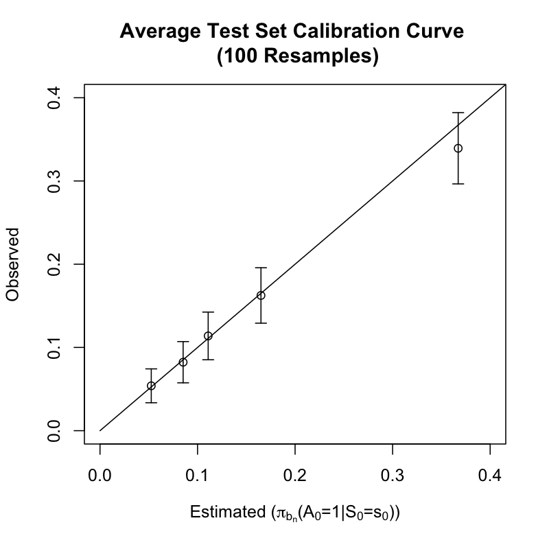
Figure 7: Real data calibration curve for the behavioral policy. We show a calibration curve for the real data, in which the estimated and observed probabilities are compared on held out data. Note that the points are chosen according to the quintiles of the distribution of the predictions. We resample the data, each time training on one half and then generating a calibration curve for the test data, and then we finally average these curves. The high concordance of the behavioral estimates, $\pi_{b_{n}}(A_{0}=1|S_{0}=s_{0})$, with the observed probabilities serves as evidence that the behavioral policy posited in Equation (2) is reasonable.

Appendix J Pseudocode

Note that the code is also provided as part of the submission and will be posted to github.

# Hashtag (#) indicates comments
Input:
    M # Number Monte-Carlo or resamples of real data
    Real dataset if not Monte-Carlo
    Lambda grid for suggested policy
    Lambda grid for behavioral policy
    X # Targeted number standard errors above behavioral value
    C # Number diverging coefficients
Repeat M times and average:
    If simulation:
        Generate data and split into test and train
    Else:
        Randomly sample real data and split into test and train
        Fit behavioral policy on training data using cv.glmnet with lambda grid for behavioral policy
        Fit a policy on training data for each lambda, using relative sparsity objective function
        Compute training and test value for each policy
        Compute training and test value variance for each policy
        Select lambda on train data
        # Useful to have one for each dataset to see distrib
        # Target value X SE above behavior with C nonbehavioral coefficients
Return:
        Set of M suggested policies # E.g., if want to inspect distribution
        Average coefficients over M datasets
        Average train and test value over M datasets
        # Will be used to select final policy on average coefficients and value


# Check the calibration of the behavioral policy
Compute (test set) average calibration curve on real data using M test-train splits
# We do not check in simulation, since we know the true generating policy

Plot distributions of M policy value, probability treatment, and relative sparsity

If real data and calibration is not reasonable:
    Break # Nehavioral policy is not well specified; do not proceed with real data analysis
Else if calibration is reasonable, or in simulation:
    Plot behavioral coefficients as horizontal lines
    Plot the suggested policy coefficients as they vary over lambda (with confidence intervals)
    Plot the train and test value as they vary over lamdba (with confidence intervals)
    Select lambda_bar on average coefficients and average value
    # Target value X SE above behavior with C nonbehavioral coefficients
    # This was done within each dataset, but here it is done on the average, which is less noisy
    Final policy is one indexed by lambda_bar
    Plot lambda_bar on value plot, visualize train value of lambda bar
    Plot lambda_bar on coefficient plot (train data), visualize number of diverging coefficients

If train data value and relative sparsity adequate
    Stop: use policy with lambda_bar
    Assess test value of policy with lambda_bar
    # Best estimate of real world value
Else:
    Increase or decrease C, X, gather more data, or reassess reward
    Start from beginning

References

- Achiam et al. (2017) Joshua Achiam, David Held, Aviv Tamar, and Pieter Abbeel. Constrained policy optimization. In International Conference on Machine Learning, pages 22–31. PMLR, 2017.
- Bellman (1957) Richard Bellman. A markovian decision process. Journal of mathematics and mechanics, pages 679–684, 1957.
- Bertsimas et al. (2016) Dimitris Bertsimas, Angela King, and Rahul Mazumder. Best subset selection via a modern optimization lens. The annals of statistics, 44(2):813–852, 2016.
- Chakraborty and Moodie (2013) Bibhas Chakraborty and Erica E. M. Moodie. Statistical Reinforcement Learning, pages 31–52. Springer New York, New York, NY, 2013. ISBN 978-1-4614-7428-9. doi: 10.1007/978-1-4614-7428-9˙3. URL https://doi.org/10.1007/978-1-4614-7428-9_3.
- Cho et al. (2020) Hunyong Cho, Shannon T Holloway, David J Couper, and Michael R Kosorok. Multi-stage optimal dynamic treatment regimes for survival outcomes with dependent censoring. arXiv preprint arXiv:2012.03294, 2020.
- Colling et al. (2018) Kristin P Colling, Kaysie L Banton, and Greg J Beilman. Vasopressors in sepsis. Surgical infections, 19(2):202–207, 2018.
- Collins et al. (2015) Gary S Collins, Johannes B Reitsma, Douglas G Altman, and Karel GM Moons. Transparent reporting of a multivariable prediction model for individual prognosis or diagnosis (tripod): the tripod statement. Journal of British Surgery, 102(3):148–158, 2015.
- de Montmollin et al. (2009) Etienne de Montmollin, Jerome Aboab, Arnaud Mansart, and Djillali Annane. Bench-to-bedside review: -adrenergic modulation in sepsis. Critical care, 13:1–8, 2009.
- DeMers and Wachs (2021) Daniel DeMers and Daliah Wachs. Physiology, mean arterial pressure. 2021.
- Der-Nigoghossian et al. (2020) Caroline Der-Nigoghossian, Drayton A Hammond, and Mahmoud A Ammar. Narrative review of controversies involving vasopressin use in septic shock and practical considerations. Annals of Pharmacotherapy, 54(7):706–714, 2020.
- Ding et al. (2022) Daisy Yi Ding, Shuangning Li, Balasubramanian Narasimhan, and Robert Tibshirani. Cooperative learning for multiview analysis. Proceedings of the National Academy of Sciences, 119(38):e2202113119, 2022.
- Du et al. (2019) Mengnan Du, Ninghao Liu, and Xia Hu. Techniques for interpretable machine learning. Communications of the ACM, 63(1):68–77, 2019.
- Ertefaie and Strawderman (2018) Ashkan Ertefaie and Robert L Strawderman. Constructing dynamic treatment regimes over indefinite time horizons. Biometrika, 105(4):963–977, 2018.
- Ertefaie et al. (2020) Ashkan Ertefaie, Nima S Hejazi, and Mark J van der Laan. Nonparametric inverse probability weighted estimators based on the highly adaptive lasso. arXiv preprint arXiv:2005.11303, 2020.
- Ertefaie et al. (2021) Ashkan Ertefaie, James R McKay, David Oslin, and Robert L Strawderman. Robust q-learning. Journal of the American Statistical Association, 116(533):368–381, 2021.
- Farahmand et al. (2016) Amir-massoud Farahmand, André MS Barreto, and Daniel N Nikovski. Value-aware loss function for model learning in reinforcement learning. 2016.
- Friedman et al. (2010) Jerome Friedman, Trevor Hastie, and Robert Tibshirani. Regularization paths for generalized linear models via coordinate descent, 2010. URL https://www.jstatsoft.org/v33/i01/.
- Futoma et al. (2020) Joseph Futoma, Michael C Hughes, and Finale Doshi-Velez. Popcorn: Partially observed prediction constrained reinforcement learning. arXiv preprint arXiv:2001.04032, 2020.
- Geevarghese III et al. (2023) Mathew Geevarghese III, Krishna Patel, Anil Gulati, and Amaresh K Ranjan. Role of adrenergic receptors in shock. Frontiers in Physiology, 14:16, 2023.
- Goldberger et al. (2000) Ary L Goldberger, Luis AN Amaral, Leon Glass, Jeffrey M Hausdorff, Plamen Ch Ivanov, Roger G Mark, Joseph E Mietus, George B Moody, Chung-Kang Peng, and H Eugene Stanley. Physiobank, physiotoolkit, and physionet: components of a new research resource for complex physiologic signals. circulation, 101(23):e215–e220, 2000.
- Gottesman et al. (2020) Omer Gottesman, Joseph Futoma, Yao Liu, Sonali Parbhoo, Leo Celi, Emma Brunskill, and Finale Doshi-Velez. Interpretable off-policy evaluation in reinforcement learning by highlighting influential transitions. In International Conference on Machine Learning, pages 3658–3667. PMLR, 2020.
- Gupta et al. (2017) Babita Gupta, Neha Garg, and Rashmi Ramachandran. Vasopressors: Do they have any role in hemorrhagic shock? Journal of anaesthesiology, clinical pharmacology, 33(1):3, 2017.
- Haneuse and Rotnitzky (2013) Sebastian Haneuse and Andrea Rotnitzky. Estimation of the effect of interventions that modify the received treatment. Statistics in medicine, 32(30):5260–5277, 2013.
- Hao et al. (2020) Botao Hao, Yaqi Duan, Tor Lattimore, Csaba Szepesvári, and Mengdi Wang. Sparse feature selection makes batch reinforcement learning more sample efficient. arXiv preprint arXiv:2011.04019, 2020.
- Harrell et al. (2001) Frank E Harrell et al. Regression modeling strategies: with applications to linear models, logistic regression, and survival analysis, volume 608. Springer, 2001.
- Hastie et al. (2009) Trevor Hastie, Robert Tibshirani, Jerome H Friedman, and Jerome H Friedman. The elements of statistical learning: data mining, inference, and prediction, volume 2. Springer, 2009.
- Hilton et al. (2021) Jacob Hilton, Karl Cobbe, and John Schulman. Batch size-invariance for policy optimization. arXiv preprint arXiv:2110.00641, 2021.
- Hoffman et al. (2011) Matthew W Hoffman, Alessandro Lazaric, Mohammad Ghavamzadeh, and Rémi Munos. Regularized least squares temporal difference learning with nested l 2 and l 1 penalization. In European Workshop on Reinforcement Learning, pages 102–114. Springer, 2011.
- Horvitz and Thompson (1952) Daniel G Horvitz and Donovan J Thompson. A generalization of sampling without replacement from a finite universe. Journal of the American statistical Association, 47(260):663–685, 1952.
- Hua et al. (2022) William Hua, Hongyuan Mei, Sarah Zohar, Magali Giral, and Yanxun Xu. Personalized dynamic treatment regimes in continuous time: a bayesian approach for optimizing clinical decisions with timing. Bayesian Analysis, 17(3):849–878, 2022.
- Johnson et al. (2016a) Alistair Johnson, Tom Pollard, and R Mark III. Mimic-iii clinical database. Physio Net, 10:C2XW26, 2016a.
- Johnson et al. (2016b) Alistair EW Johnson, Tom J Pollard, Lu Shen, Li-wei H Lehman, Mengling Feng, Mohammad Ghassemi, Benjamin Moody, Peter Szolovits, Leo Anthony Celi, and Roger G Mark. Mimic-iii, a freely accessible critical care database. Scientific data, 3(1):1–9, 2016b.
- Johnson et al. (2016c) Alistair EW Johnson, Tom J Pollard, Lu Shen, H Lehman Li-Wei, Mengling Feng, Mohammad Ghassemi, Benjamin Moody, Peter Szolovits, Leo Anthony Celi, and Roger G Mark. Mimic-iii, a freely accessible critical care database. Scientific data, 3(1):1–9, 2016c.
- Jones et al. (2022) Jeremiah Jones, Ashkan Ertefaie, and Robert L Strawderman. Valid post-selection inference in robust q-learning. arXiv preprint arXiv:2208.03233, 2022.
- Kennedy (2019) Edward H Kennedy. Nonparametric causal effects based on incremental propensity score interventions. Journal of the American Statistical Association, 114(526):645–656, 2019.
- Kennedy (2022) Edward H Kennedy. Semiparametric doubly robust targeted double machine learning: a review. arXiv preprint arXiv:2203.06469, 2022.
- Kolter and Ng (2009) J Zico Kolter and Andrew Y Ng. Regularization and feature selection in least-squares temporal difference learning. In Proceedings of the 26th annual international conference on machine learning, pages 521–528, 2009.
- Komorowski et al. (2018) Matthieu Komorowski, Leo A Celi, Omar Badawi, Anthony C Gordon, and A Aldo Faisal. The artificial intelligence clinician learns optimal treatment strategies for sepsis in intensive care. Nature medicine, 24(11):1716–1720, 2018.
- Lee et al. (2012) Joon Lee, Rishi Kothari, Joseph A Ladapo, Daniel J Scott, and Leo A Celi. Interrogating a clinical database to study treatment of hypotension in the critically ill. BMJ open, 2(3):e000916, 2012.
- Lipton (2018) Zachary C Lipton. The mythos of model interpretability: In machine learning, the concept of interpretability is both important and slippery. Queue, 16(3):31–57, 2018.
- Liu et al. (2012) Bo Liu, Sridhar Mahadevan, and Ji Liu. Regularized off-policy td-learning. Advances in Neural Information Processing Systems, 25:836–844, 2012.
- Liu et al. (2019) Zhuang Liu, Xuanlin Li, Bingyi Kang, and Trevor Darrell. Regularization matters in policy optimization–an empirical study on continuous control. arXiv preprint arXiv:1910.09191, 2019.
- Luckett et al. (2019) Daniel J Luckett, Eric B Laber, Anna R Kahkoska, David M Maahs, Elizabeth Mayer-Davis, and Michael R Kosorok. Estimating dynamic treatment regimes in mobile health using v-learning. Journal of the American Statistical Association, 2019.
- Marín (1995) Jesús Marín. Age-related changes in vascular responses: a review. Mechanisms of ageing and development, 79(2-3):71–114, 1995.
- Miller (2019) Tim Miller. Explanation in artificial intelligence: Insights from the social sciences. Artificial intelligence, 267:1–38, 2019.
- Muñoz and van der Laan (2012) Iván Díaz Muñoz and Mark van der Laan. Population intervention causal effects based on stochastic interventions. Biometrics, 68(2):541–549, 2012.
- Murphy (2003) Susan A Murphy. Optimal dynamic treatment regimes. Journal of the Royal Statistical Society: Series B (Statistical Methodology), 65(2):331–355, 2003.
- Murphy et al. (2001) Susan A Murphy, Mark J van der Laan, James M Robins, and Conduct Problems Prevention Research Group. Marginal mean models for dynamic regimes. Journal of the American Statistical Association, 96(456):1410–1423, 2001.
- Natarajan (1995) Balas Kausik Natarajan. Sparse approximate solutions to linear systems. SIAM journal on computing, 24(2):227–234, 1995.
- Ng and Jordan (2013) Andrew Y Ng and Michael I Jordan. Pegasus: A policy search method for large mdps and pomdps. arXiv preprint arXiv:1301.3878, 2013.
- Ng and Russell (2000) Andrew Y Ng and Stuart J Russell. Algorithms for inverse reinforcement learning. In Icml, volume 1, page 2, 2000.
- Niculescu-Mizil and Caruana (2005) Alexandru Niculescu-Mizil and Rich Caruana. Predicting good probabilities with supervised learning. In Proceedings of the 22nd international conference on Machine learning, pages 625–632, 2005.
- Precup (2000) Doina Precup. Eligibility traces for off-policy policy evaluation. Computer Science Department Faculty Publication Series, page 80, 2000.
- Price (2014) Brad Scott Price. Fusion Penalties in Statistical Learning. PhD thesis, University of Minnesota, 2014.
- Puiutta and Veith (2020) Erika Puiutta and Eric Veith. Explainable reinforcement learning: A survey. In International cross-domain conference for machine learning and knowledge extraction, pages 77–95. Springer, 2020.
- Puterman (2014) Martin L Puterman. Markov decision processes: discrete stochastic dynamic programming. John Wiley & Sons, 2014.
- Qin et al. (2014) Zhiwei Qin, Weichang Li, and Firdaus Janoos. Sparse reinforcement learning via convex optimization. In International Conference on Machine Learning, pages 424–432. PMLR, 2014.
- Raghu et al. (2017) Aniruddh Raghu, Matthieu Komorowski, Leo Anthony Celi, Peter Szolovits, and Marzyeh Ghassemi. Continuous state-space models for optimal sepsis treatment-a deep reinforcement learning approach. arXiv preprint arXiv:1705.08422, 2017.
- Ramachandran and Amir (2007) Deepak Ramachandran and Eyal Amir. Bayesian inverse reinforcement learning. In IJCAI, volume 7, pages 2586–2591, 2007.
- Robins et al. (1994) James M Robins, Andrea Rotnitzky, and Lue Ping Zhao. Estimation of regression coefficients when some regressors are not always observed. Journal of the American statistical Association, 89(427):846–866, 1994.
- Rudin (2019) Cynthia Rudin. Stop explaining black box machine learning models for high stakes decisions and use interpretable models instead. Nature Machine Intelligence, 1(5):206–215, 2019.
- Rudrapatna et al. (2020) Vivek A Rudrapatna, Benjamin S Glicksberg, Patrick Avila, Emily Harding-Theobald, Connie Wang, and Atul J Butte. Accuracy of medical billing data against the electronic health record in the measurement of colorectal cancer screening rates. BMJ open quality, 9(1):e000856, 2020.
- Russell et al. (2021) James A Russell, Anthony C Gordon, Mark D Williams, John H Boyd, Keith R Walley, and Niranjan Kissoon. Vasopressor therapy in the intensive care unit. In Seminars in Respiratory and Critical Care Medicine, volume 42, pages 059–077. Thieme Medical Publishers, Inc., 2021.
- Schulman et al. (2015) John Schulman, Sergey Levine, Pieter Abbeel, Michael Jordan, and Philipp Moritz. Trust region policy optimization. In International conference on machine learning, pages 1889–1897. PMLR, 2015.
- Schulte et al. (2014) Phillip J Schulte, Anastasios A Tsiatis, Eric B Laber, and Marie Davidian. Q-and a-learning methods for estimating optimal dynamic treatment regimes. Statistical science: a review journal of the Institute of Mathematical Statistics, 29(4):640, 2014.
- Smith and Maani (2021) Matthew D Smith and Christopher V Maani. Norepinephrine. In StatPearls [Internet]. StatPearls Publishing, 2021.
- Song et al. (2015) Rui Song, Weiwei Wang, Donglin Zeng, and Michael R Kosorok. Penalized q-learning for dynamic treatment regimens. Statistica Sinica, 25(3):901, 2015.
- Standl et al. (2018) Thomas Standl, Thorsten Annecke, Ingolf Cascorbi, Axel R Heller, Anton Sabashnikov, and Wolfram Teske. The nomenclature, definition and distinction of types of shock. Deutsches Ärzteblatt International, 115(45):757, 2018.
- Steyerberg et al. (2010) Ewout W Steyerberg, Andrew J Vickers, Nancy R Cook, Thomas Gerds, Mithat Gonen, Nancy Obuchowski, Michael J Pencina, and Michael W Kattan. Assessing the performance of prediction models: a framework for some traditional and novel measures. Epidemiology (Cambridge, Mass.), 21(1):128, 2010.
- Sutton and Barto (2018) Richard S Sutton and Andrew G Barto. Reinforcement learning: An introduction. 2018.
- Thomas (2015) Philip S Thomas. Safe reinforcement learning. PhD thesis, 2015.
- Tibshirani (2011) Robert Tibshirani. Regression shrinkage and selection via the lasso: a retrospective. Journal of the Royal Statistical Society: Series B (Statistical Methodology), 73(3):273–282, 2011.
- Tibshirani et al. (2005) Robert Tibshirani, Michael Saunders, Saharon Rosset, Ji Zhu, and Keith Knight. Sparsity and smoothness via the fused lasso. Journal of the Royal Statistical Society: Series B (Statistical Methodology), 67(1):91–108, 2005.
- Van Calster et al. (2016) Ben Van Calster, Daan Nieboer, Yvonne Vergouwe, Bavo De Cock, Michael J Pencina, and Ewout W Steyerberg. A calibration hierarchy for risk models was defined: from utopia to empirical data. Journal of clinical epidemiology, 74:167–176, 2016.
- van der Vaart (2000) Aad W van der Vaart. Asymptotic statistics, volume 3. Cambridge university press, 2000.
- Watkins and Dayan (1992) Christopher JCH Watkins and Peter Dayan. Q-learning. Machine learning, 8:279–292, 1992.
- Yang et al. (2019) Wenhao Yang, Xiang Li, and Zhihua Zhang. A regularized approach to sparse optimal policy in reinforcement learning. Advances in Neural Information Processing Systems, 32:5940–5950, 2019.
- Yao et al. (2022) Jiayu Yao, Sonali Parbhoo, Weiwei Pan, and Finale Doshi-Velez. Policy optimization with sparse global contrastive explanations. arXiv preprint arXiv:2207.06269, 2022.
- Yapps et al. (2017) Bryce Yapps, Sungtae Shin, Ramin Bighamian, Jill Thorsen, Colleen Arsenault, Sadeq A Quraishi, Jin-Oh Hahn, and Andrew T Reisner. Hypotension in icu patients receiving vasopressor therapy. Scientific reports, 7(1):1–10, 2017.
- Young et al. (2014) Jessica G Young, Miguel A Hernán, and James M Robins. Identification, estimation and approximation of risk under interventions that depend on the natural value of treatment using observational data. Epidemiologic methods, 3(1):1–19, 2014.