Bayesian inference for aggregated Hawkes processes

Abstract

The Hawkes process, a self-exciting point process, has a wide range of applications in modeling earthquakes, social networks and stock markets. The established estimation process requires that researchers have access to the exact time stamps and spatial information. However, available data are often rounded or aggregated. We develop a Bayesian estimation procedure for the parameters of a Hawkes process based on aggregated data. Our approach is developed for temporal, spatio-temporal, and mutually exciting Hawkes processes where data are available over discrete time periods and regions. We show theoretically that the parameters of the Hawkes process under different specifications are identifiable from aggregated data, and demonstrate the method on simulated temporal and spatio-temporal data with various model specifications in the presence of one or more interacting processes, and under varying coarseness of data aggregation. Finally, we analyze spatio-temporal point pattern data of insurgent attacks in Iraq from October to December 2006, and we find coherent results across different time and space aggregations.

Introduction

Point pattern data are ubiquitous across a number of applied fields, and understanding the underlying dynamics generating these patterns is the goal of point pattern modeling. A type of dynamic that is often of explicit interest is that of self-excitement, referring to the case where the occurrence of an event triggers subsequent events. A common model for studying excitement in point pattern data is the Hawkes process (Hawkes, 1971). With initial application in seismology (Ogata, 1998), Hawkes processes have been used to study terrorist attacks (Porter and White, 2012; Lewis et al., 2012), financial markets (Lapham, 2014) and in epidemiology (Chiang et al., 2022), among other areas. Their wide use and applicability has led to extensive research on precise and computationally efficient estimation of model parameters, within the frequentist (Veen and Schoenberg, 2008) and the Bayesian (Rasmussen, 2013) paradigm. In addition to the exact time of an event’s occurrence, researchers often have access to specific characteristics of the event. In this manuscript, we focus on the scenario where an event’s location might also be available. Incorporating an event’s spatial coordinates in the point process modeling can provide additional insights in the process’ self-excitement dynamics. In addition to studying self-excitement, the Hawkes process can incorporate mutual excitement among multiple point processes of different types. Mutually-exciting Hawkes processes provide a framework to study interaction dynamics where the occurrence of an event of one type can lead to subsequent events of the same or the other type.

Standard estimation techniques for the Hawkes process require that the exact time and location of events is known. However, real data are often only available at aggregated levels across time and space. For example, the time of occurrence of an event might be coarsened at the day level rather than knowing the exact time stamp, and some published earthquake data are aggregated over towns. Since data of this form are available within bins of time and space they could also be referred to as binned or discretized, though we maintain the term aggregated for the remainder of this manuscript. When data are aggregated, standard estimation and inference techniques for the underlying continuous time and space Hawkes point process are not applicable. In these cases, it is common practice to model the discretized point pattern dynamics using, for example, autoregressive models in time or space (Aldor-Noiman et al., 2016; Darolles et al., 2019). These models could in principle perform adequately for forecasting event counts, but they can only do so over intervals that are multiples of the data’s aggregation size. More importantly, since they ignore the possible dependencies among events within the discrete bins, they are not useful for learning the process dynamics at the scale at which they naturally occur, which is often of explicit interest. Even though there exists some work on inferring the underlying Hawkes process model parameters from discrete-time models based on temporal, aggregated point pattern data (Kirchner, 2016, 2017), the equivalence is only established for autoregressive models with infinite lags (which are impossible to fit), and it is not clear whether the results are sensitive to the scale of data aggregation or how the method can be extended to incorporate space, other marks, or multiple processes. Shlomovich et al. (2022) proposed a Monte Carlo Expectation-Maximization (MC-EM) algorithm to estimate the parameters of a Hawkes process based on aggregated temporal data, and Shlomovich et al. (2021) extended it to multivariate Hawkes processes. Their approach, which is only developed for temporal point patterns, is based on an expectation-maximization algorithm which cannot be used directly for performing inference over model parameters.

In this manuscript, we propose an estimation technique for modeling point pattern data within the realm of Hawkes processes when the available data are aggregated across time, space, or both. We review the Hawkes process in Section 2. We turn our attention to aggregated point pattern data in Section 3. We show theoretically that the parameters of a Hawkes process are identifiable from aggregated data under various model specifications. We introduce our approach, which is positioned within the Bayesian paradigm, and it is based on considering the real (continuous) time an event occurrence as a latent variable. We propose a Markov Chain Monte Carlo (MCMC) scheme for learning the parameters of the Hawkes process which involves straightforward imputation of these latent variables. Our approach improves on the existing methodology in a number of ways. First, by placing our approach within the Bayesian framework, our estimation strategy leads to straightforward inference procedures that propagate all sources of uncertainty. Second, it allows for aggregated point pattern data with spatial information, which can itself be available at coarse spatial regions. Lastly, it allows for modeling multiple, mutually-exciting Hawkes processes, each of which can be aggregated across time, space, or both, with the same or different granularity. Under similar model specifications used in Tucker et al. (2019), we evaluate the performance of the proposed approach in terms of estimation and inference over simulated data sets (Section 4), and using real data on insurgent violence in Iraq (Section 5), under different coarseness of aggregation in time and space. We conclude with a discussion and possible extensions in Section 6.

The Hawkes process

We review the temporal Hawkes process in Section 2.1, the spatio-temporal Hawkes process in Section 2.2, and the multivariate Hawkes process in Section 2.3.

The temporal Hawkes process

Hawkes processes are a class of point processes which exhibit a self-exciting behavior, meaning that the occurrence of an event can lead to the occurrence of additional, subsequent events. Consider a temporal point process with event times $\{t_{i}\}$. Let $N$ be the corresponding counting measure for the process on $\mathbb{R}$ which counts the number of points falling within any arbitrary Borel set. Let $\mathcal{H}_{t}$ denote the process’ history up to time $t$, $\mathcal{H}_{t}=\{t_{i}:t_{i}<t\}$. The process’ mechanisms are often characterized through its (conditional) intensity, defined as the limit of the expected number of points in an infinitesimal time window following $t$ given the realized history $\mathcal{H}_{t}$ (Daryl and Vere-Jones, 2003),

$$\lambda^{*}(t)=\lim_{\Delta t\downarrow 0}\frac{\textrm{E}[\ \textrm{N}\{(t,t+\Delta t)\}\mid\mathcal{H}_{t}]}{\Delta t}.$$

For the temporal Hawkes process, the conditional intensity is of the form

$$\lambda^{*}(t)=\mu(t)+\ \sum_{\makebox[0.0pt]{$\scriptstyle t_{i}\in\mathcal{H}_{t}$}}\alpha\ g(t-t_{i}),$$ (1)

The superscript ^∗ denotes that the intensity is defined conditional on the history. The function $\mu(t)$ is a non-negative function which is usually assumed to be constant. In turn, $g(t)$ is a density function on $[0,\infty)$, and common choices are the exponential and Lomax densities (see Table 1), the latter of which specifies the Epidemic Type Aftershock Sequences (ETAS) model in seismology (Ogata, 1998). The parameter $\alpha$ needs to satisfy that $\alpha\in(0,1)$ for the stationarity of the process.

An alternative formalization of the Hawkes process that will be useful moving forward views the Hawkes process as a Poisson cluster process (Hawkes and Oakes, 1974). From this point of view, an event is either an immigrant that occurred in the system separately from previous events, or an offspring of a previous event which occurred due to the process’ self-excitement. The set of these relations is called the process’ branching structure. We denote event $j$’s (latent) branching information as $Y_{j}$, where $Y_{j}=0$ if $t_{j}$ is an immigrant and $Y_{j}=i$ if $t_{j}$ is an offspring of event $i$. The collection of this information across all events is denoted by $\bm{Y}$. Under the Poisson cluster representation of the Hawkes process, a realization of the process can be thought of as occurring in the following manner. First, the set of all immigrants $I=\{t_{i}:Y_{i}=0\}$ (or “generation 0") are generated from a Poisson process with $\lambda_{I}(t)=\mu(t)$. Then, each of the immigrant events $t_{i}\in I$ can give rise to offspring events $O_{i}=\{t_{j}:Y_{j}=i\}$ in generation 1. Events in $O_{i}$ are generated as a Poisson process with intensity $\lambda_{O_{i}}(t)=\alpha g(t-t_{i})$. At the next step, each event in generation 1 could lead to events in generation 2 in the same manner, and that continues on. Due to this representation, $\mu(t)$ and $\alpha g(t)$ are called background and offspring intensity, respectively. This representation also illustrates that $\alpha$ represents the mean number of offsprings of an event, and $g(t)$ is the density function specifying the length of the time interval between an offspring and its parent.

For our discussion in Section 3, it is useful to introduce the likelihood of an observed point pattern $\bm{x}$ and branching structure $\bm{Y}$ during a time period $[0,T)$ under the Hawkes model. If $\theta$ is the vector of all parameters, then

$$p(\bm{x},\bm{Y}|\theta) =p(I|\bm{Y},\theta)\prod_{i=1}^{n}p(O_{i}|\bm{Y},\theta)$$ (2)

$$=\exp(-M(T))\prod_{t_{i}\in I}\mu(t_{i})\prod_{i=1}^{n}\Big{\{}\exp(-\alpha G(T-t_{i}))\prod_{t_{j}\in O_{i}}\alpha g(t_{j}-t_{i})\Big{\}},$$

where $M(T)=\int_{0}^{T}\mu(t)\,\mathrm{d}t$, and $G(T-t_{i})=\int_{0}^{T-t_{i}}g(t)\,\mathrm{d}t$.

The spatio-temporal Hawkes process

When the locations of the events are available, the observed point process is of the form $\bm{x}=\{(t_{i},s_{i}):i=1,2,\dots,n\}$, where $t_{i}$ and $s_{i}$ denote the time and location of the event $i$. The conditional intensity to predict the rate of events at time $t\in[0,T)$ and location $s\in W\subset\mathbb{R}^{2}$ can be defined in the similar way to that for temporal processes:

$$\lambda^{*}(t,s)=\lim_{\Delta s,\Delta t\downarrow 0}\frac{\textrm{E}[\ \textrm{N}\{(t,t+\Delta t)\times B(s,\Delta s)\}\mid\mathcal{H}_{t}]}{\Delta t|B(s,\Delta s)|},$$

where $N$ is now the counting measure over $[0,T)\times W$, $|B(s,\Delta_{s})|$ is the Lebesgue measure of the ball $B(s,\Delta s)$, and $\mathcal{H}_{t}=\{(t_{i},s_{i}):t_{i}<t\}.$ A spatio-temporal Hawkes process is one whose conditional intensity is of the form

$$\lambda^{*}(t,s)=u(t,s)+\ \sum_{\makebox[0.0pt]{$\scriptstyle(t_{i},s_{i})\in\mathcal{H}_{t}$}}\alpha\ g(t-t_{i},s-s_{i}),$$

where $g(t,s)$ is a density function on $\mathbb{R}\times\mathbb{R}^{2}$. As discussed in Reinhart (2018), $u(t,s)$ is usually assumed to be time homogeneous, $u(t,s)=u(s)$, and the triggering function $g(t,s)$ is often taken to be the product of time and spatial components: $g(t,s)=g_{1}(t)g_{2}(s)$. We adopt this throughout the paper, and consider

$$\lambda^{*}(t,s)=\mu f(s)+\ \sum_{\makebox[0.0pt]{$\scriptstyle(t_{i},s_{i})\in\mathcal{H}_{t}$}}\alpha\ g_{1}(t-t_{i})g_{2}(s-s_{i}),$$

where $\mu\geq 0$ is a constant and $f(s)$ is a probability density function on $\mathbb{R}^{2}.$ Common choices for $g_{2}(s)$ include the bivariate Gaussian and the power law distribution (Ogata, 1998) (see Table 1).

Table 1: Common choices for $g_{1}(t)$ and $g_{2}(s)$. The ones considered in this manuscript are marked with an asterisk. For the temporal models, $g(t)=g_{1}(t).$

$g_{1}(t)$		$g_{2}(s)$
Exponential∗	Lomax∗	Gaussian∗	Power Law
$\beta\exp(-\beta t)$	$\displaystyle\frac{(p-1)c^{p-1}}{(t+c)^{p}}$	$\displaystyle\frac{1}{2\pi\gamma^{2}}\exp(-\frac{||s||^{2}}{2\gamma^{2}})$	$\displaystyle\frac{(q-1)d^{q-1}}{\pi(||s||^{2}+d)^{q}}$

As in the temporal case, the spatio-temporal Hawkes process can also be viewed as a Poisson cluster process: the set of all immigrant $I$ are generated from a nonhomogeneous Poisson process with intensity $\lambda_{I}(t,s)=\mu f(s)$, and each offspring $(t_{i},s_{i})$ produces a nonhomogeneous Poisson process $O_{i}$ with intensity $\lambda_{O_{i}}(t,s)=\alpha g(t-t_{i},s-s_{i}).$ The likelihood of a spatio-temporal Hawkes process on $[0,T)\times W$ can be written as

$$p(\bm{x},\bm{Y}|\theta) =\exp\Big{(}-\int_{0}^{T}\!\!\!\int_{W}\lambda_{I}(t,s))\,\text{d}s\,\text{d}t\Big{)}\prod_{t_{i}\in I}\lambda_{I}(t_{i},s_{i})$$ (3)

$$\hskip 10.0pt\times\prod_{i=1}^{n}\exp\Big{(}-\int_{0}^{T}\!\!\!\int_{W}\lambda_{O_{i}}(t,s))\,\text{d}s\,\text{d}t\Big{)}\prod_{t_{j}\in O_{j}}\lambda_{O_{i}}(t_{j},s_{j}).$$

The integrals in Equation 3 may be difficult to evaluate. When the observation window $W$ is sufficiently large, the likelihood can be approximated by

$$p(\bm{x},\bm{Y}|\theta)=\exp(-\mu T)\mu^{|I|}\prod_{i\in I}f(s_{i})\prod_{i=1}^{n}\Big{\{}\exp(-\alpha G_{1}(T-t_{i}))\prod_{t_{j}\in O_{i}}\alpha g_{1}(t_{j}-t_{i})\Big{\}},$$ (4)

where $G_{1}(T-t_{i})=\int_{0}^{T-t_{i}}g_{1}(t)\,\mathrm{d}t$. This approximation is advocated in Reinhart (2018) and Schoenberg (2013).

Multivariate Hawkes process

The Hawkes process has been extended to accommodate multiple processes with mutually exciting behavior. An $L$-dimensional spatio-temporal process gives rise to point patterns of the form $\{(t_{l,i},s_{l,i}):l\in\{1,\dots L\},i\in\mathbb{N}\},$ where $t_{l,i}$ and $s_{l,i}$ are the time and location of the $i^{th}$ event from process $l$. The multivariate Hawkes process can be defined through the respective conditional intensity of each of its $L$ components:

$$\lambda_{l}^{*}(t,s)=\mu_{l}f_{l}(s)+\sum_{m=1}^{L}\sum_{t_{l,i}<t}\alpha_{m,l}g_{1,m,l}(t-t_{l,i})g_{2,m,l}(s-s_{l,i}),$$ (5)

where $l=1,2,\dots,L$, and (implicitly) the history is now extended to include times and locations for the events occurring before time $t$ from all $L$ processes. Similar to the univariate case, a multivariate Hawkes process can be viewed as a Poisson cluster process generated by a latent branching structure $\bm{Y}=\{Y_{l,i}\}$ where $Y_{l,j}=(0,0)$ if $t_{l,j}$ is an immigrant and $Y_{l,j}=(k,i)$ if $t_{l,j}$ is an offspring of $t_{k,i}$ (see also Appendix B). Through this equivalence, we can conceive $\mu_{l}f_{l}(s)$ as the background intensity for process $l$ and $\alpha_{m,l}g_{1,m,l}(t-t_{l,i})g_{2,m,l}(s-s_{l,i})$ as the offspring intensity corresponding to either self-excitation ($m=l$) or external-excitation ($m\neq l$).

Aggregated Hawkes process

Standard estimation techniques for the parameters of the Hawkes process require that the available data include exact information on the time and characteristics of the events. However, in many situations researchers only have access to some limited information about the events: they might know the date or region an event occurred, without having access to its precise time stamp or location. We refer to such data as “aggregated” point pattern data, and we consider estimation of parameters of the underlying process when the underlying exact event occurrence follows a Hawkes process.

In this section, we introduce the proposed Bayesian approach for estimating the parameters in spatio-temporal Hawkes processes when aggregation occur over time, space, or both. We introduce aggregated point patterns in Section 3.1, and we link them to the exact, latent point pattern data in Section 3.2, which is the basis of our approach. In Section 3.3, we show that the true underlying Hawkes process model is identifiable based on aggregated temporal or spatio-temporal data. We introduce the models that we consider in Section 3.4 and give details about the MCMC steps in Section 3.5.

Aggregated event information

We consider three scenarios of aggregated data from Hawkes processes of increasing complexity. Aggregated temporal event data, aggregated spatio-temporal event data, and the scenario with aggregated event data on multiple processes. We assume that the process is observed during the $[0,T)$ time window, and, if spatial information is available, over a spatial window $W=[0,W_{x}]\times[0,W_{y}]$. We consider a rectangular spatial window here for notational simplicity, though our approach could be applied to spatial windows of any shape (such as the one in Section 5).

For aggregated temporal data, the time interval $[0,T)$ is partitioned into $n_{1}$ bins $B^{t}_{1},B^{t}_{2},\dots,B^{t}_{n_{1}}$. Then, the observed data correspond to the number of events that occurred within each temporal bin, denoted by $N_{1},N_{2},\dots,N_{n_{1}}\in\{0\}\cup\mathbb{Z}^{+}$. For aggregated spatio-temporal data, the spatial window is also partitioned in $n_{2}$ bins, $B^{s}_{1},B^{s}_{2},\dots,B^{s}_{n_{2}}$. In this case, the observed data are of the form $\{N_{i,j}:i=1,2,\dots,n_{1},j=1,2,\dots,n_{2}\}$, where $N_{i,j}$ denotes the number of events in $B^{t}_{i}\times B^{s}_{j}.$ We consider temporal bins of equal size $\Delta^{t}$, and that the spatial locations are aggregated on a grid sharing the same length $\Delta^{s}$. Therefore, in what follows we have $B^{t}_{i}=[(i-1)\Delta^{t},i\Delta^{t})$ and $B^{s}_{j}$ is of the form $[(k-1)\Delta^{s},k\Delta^{s})\times[(m-1)\Delta^{s},m\Delta^{s})$ for some $k,m\in\mathbb{N}.$ We refer to $\Delta^{t}$ and $\Delta^{s}$ as the size of aggregation in time and space, respectively. A visualization of aggregated spatio-temporal data is shown in Figure 1. We maintain time and space bins of equal size for notational simplicity, however it is easy to modify our approach for more complicated settings with unequal bin lengths in time or irregular shapes in space.

When there are $L$ processes, the aggregation sizes in time and space for each process may be different. We denote the aggregation sizes in time and space for process $l$ by $\Delta^{t}_{l}$ and $\Delta^{s}_{l}$, respectively, and the spatio-temporal bins by $B^{t}_{l,i}\times B^{s}_{l,j}:i=1,2,\dots,n_{l,1},j=1,2,\dots,n_{l,2}$. Then, the aggregated data for multiple processes are in the form $\{N_{l,i,j}:\text{all }l,i,j\}$ where $N_{l,i,j}$ is the number of events from process $l$ in $B^{t}_{l,i}\times B^{s}_{l,j}.$

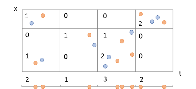
$\downarrow$

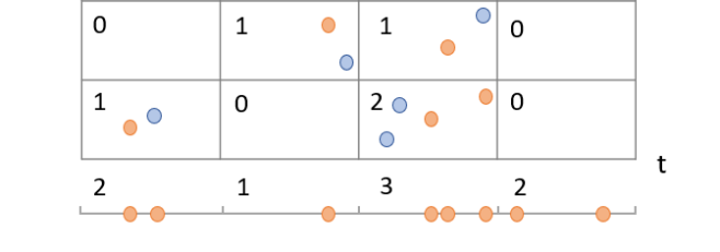
Figure 1: Exact and Aggregated Point Pattern Data. The orange points represent the exact spatio-temporal (top) or temporal (bottom) data. The continuous time (horizontal axis) is divided in four time bins, and the continuous space (one-dimensional, vertical axis) is divided in three bins. The aggregated data correspond to the count of events occurring within each bin, which might be available with spatial information on the $3\times 4$ spatio-temporal bins (top), and without spatial information on the 4 temporal bins (bottom). The blue points represent an alternative point pattern that would match the same aggregated data.

Latent variable formulation

Even though available data are in aggregated form, the events truly occur in continuous time and space, and ignoring dependencies among events in the same bin can lead to misleading conclusions. Instead, our approach models the aggregated event data at the scale they actually occur, on continuous time and space. The main idea is to consider the exact time and location of an event as latent variables.

We focus here on spatio-temporal aggregated data from a univariate process, $\bm{N}=\{N_{i,j}:i=1,2,\dots,n_{1},j=1,2,\dots,n_{2}\}$. We consider $\bm{x}=\{(t_{i},s_{i}):i=1,2,\dots,n\}$, which represents the underlying exact point pattern which is unobserved. If $\theta$ represents the parameters of the Hawkes process driving $\bm{x}$, we write the likelihood of the observed data given the parameters of the Hawkes process as

$$p(\bm{N}\mid\theta)=\int p(\bm{N},\bm{x},\bm{Y}\mid\theta)\ \mathrm{d}\bm{x}\ \mathrm{d}\bm{Y},$$ (6)

integrating over the distribution of the latent exact point pattern $\bm{x}$ and its latent branching structure $\bm{Y}$ (discussed in Section 2).

This can be further simplified. Each exact point pattern $\bm{x}$ maps to a single aggregated point pattern $\bm{N}$. Thus, it holds that $p(\bm{N}\mid\bm{x},\bm{Y},\theta)=p(\bm{N}\mid\bm{x})$, which is equal to 1 only when the aggregated data match the exact point pattern in terms of the total number of events and the number of events in each bin. Therefore,

$$p(\bm{N}\mid\bm{x},\bm{Y},\theta)=\begin{cases}1,&\text{if }\sum_{k=1}^{n}1{\{(t_{k},s_{k})\in B^{t}_{i}\times B^{s}_{j}\}}=N_{i,j}\text{ for all }i,j\\[5.0pt] 0,&\text{otherwise.}\end{cases}$$ (7)

Given the process’ parameters, the exact point pattern with the branching structure follows the distribution given in Equation 3. Therefore, the likelihood of an aggregated point pattern in Equation 6 can be written as $\int p(\bm{x},\bm{Y}\mid\theta)\ \mathrm{d}\bm{x}\ \mathrm{d}\bm{Y}$, where the integral is over exact point patterns that agree with the aggregated one. As an example, Figure 1 shows two exact point patterns that lead to the same aggregated data.

Similar arguments hold for a temporal process or a multivariate spatio-temporal process. This formulation is simplified in the case of a temporal process, and extended in the case of multiple spatio-temporal processes, though we refrain from presenting the details here (we refer interested readers to Appendix B).

Identifiability of the Hawkes process based on aggregated data

One question we need to address is the identifiability of the model parameters when parts of the information is lost due to the aggregation. In Theorems 3.1 and 3.2 below, we establish that the parameters of the temporal and spatio-temporal Hawkes process, respectively, can be recovered from the observed aggregated data under different specifications of the model’s functional form.

Theorem 3.1 (Identifiability for aggregated temporal data).

Let $\{t_{1},t_{2},\dots,t_{n}\}$ be a temporal Hawkes process on $[0,T)$ defined by intensity $\lambda_{\theta}^{*}(t)=\mu+\sum_{t_{i}<t}\alpha g(t-t_{i}),$ where $\theta$ is the vector of parameters. Let $\bm{B}=\{B_{1},B_{2},\dots,B_{k}\}$ be temporal bins with equal bin length $\Delta$ and $k\geq 3$. If $g(t)$ is the exponential or Lomax density function defined in Table 1, then the corresponding aggregated Hawkes process model is identifiable based on aggregated data $N_{1},N_{2},\dots,N_{k}$.

Theorem 3.2 (Identifiability for aggregated spatio-temporal data).

Let $\{(t_{i},s_{i}):i=1,2,\dots,n\}$ be a spatio-temporal Hawkes process on $[0,T)\times W$ defined by intensity $\lambda_{\theta}^{*}(t,s)=\mu f(s)+\sum_{t_{i}<t}\alpha g_{1}(t-t_{i})g_{2}(s-s_{i}),$ where $f(s)$ is known, and $\theta$ is the vector containing $\mu,\alpha$ and parameters in $g_{1}(t)$ and $g_{2}(s).$ Let $\bm{B}=\{B_{i}^{t}\times B_{j}^{s}:1\leq i\leq k_{1},1\leq j\leq k_{2}\}$ be spatio-temporal bins with equal time bin length $\Delta^{t}$ and space bin length $\Delta^{s}$. Let $\bm{N}=\{N_{i,j}:1\leq i\leq k_{1},1\leq j\leq k_{2}\}$ be the corresponding aggregated spatio-temporal Hawkes process. Suppose

1. $g_{1}(t)$ is the exponential or Lomax desntiy function,

2. $g_{2}(s)$ is the bivariate Gaussian density,

3. $W=\mathbb{R}^{2}$ and $f(s)$ is either known or does not include additional parameters, and

4. $k_{1}\geq 3$ and $\Delta^{s}<\infty$, i.e. there is at least three time bins and the spatial bins have finite length,

then the parameters of the Hawkes process are identifiable based on the aggregated data.

The proofs are included in Appendix C. There, we also provide an identifiability result for non-constant background intensity $\mu(t)$. The proof provides an interesting insight: the identifiability of the parameters in the excitation function is based on the triggering effect of one event in different time bins. Therefore, for Hawkes processes for which most parent-offspring pairs fall in the same aggregation bin, the parameters may be weakly identifiable based on the aggregated data, even though the theoretical identifiability can be achieved.

Parametric specifications of the Hawkes model in this manuscript

Hawkes process models are flexible and there are many other choices for $\mu(t)$, $g_{1}(t)$, $g_{2}(s)$ and $f(s).$ In Section 3.3, we showed that the Hawkes process model is identifiable based on temporal or spatio-temporal data with exponential or Lomax density for the time component and Gaussian density for the spatial component of the triggering function. We also showed an extension for non-constant background intensity.

For simplicity, we specify that the occurrence of immigrants is homogeneous in time by specifying $\mu(t)=\mu 1{\{t\geq 0\}}$ moving forward. For spatio-temporal data, we assume that the background intensity is homogeneous over the region $W$ for most of the manuscript, and $f(s)=|W|^{-1}{1{\{s\in W\}}}$, where $|W|$ is the area of the spatial window. We extend this in Section 5 where we considered a spatio-temporal model with a non-homogeneous background intensity over space.

We consider forms of the excitation function as displayed in Table 1. We mainly focus on the exponential density with rate parameter $\beta$ for the time component (mean $1/\beta$), and we focus on the bivariate Gaussian density for the spatial component. For the multivariate Hawkes process, we maintain these specifications while allowing for different parameters for each component of the process. Most parametric alternatives are straightforward to implement within our framework. We analyze Hawkes processes with the Lomax offspring kernel in the Appendix.

Estimation and inference within the Bayesian framework

We propose a Bayesian approach to estimate the parameters of the Hawkes process, $\theta$, based on aggregated point pattern data. Given a prior on the model parameters, the proposed approach acquires their posterior distribution, $p(\theta\mid\bm{N})$ based on the likelihood in Equation 6, by integrating out the exact Hawkes point pattern and corresponding branching structure from their joint posterior distribution $p(\bm{x},\bm{Y},\theta\mid\bm{N})$. We approximate the joint posterior distribution of $(\bm{x},\bm{Y},\theta)$ using MCMC methods, by iteratively imputing the exact point pattern, and updating the model parameters given the imputed exact data. Bayesian approaches that augment their sampling scheme using latent variables in an iterative manner have been previously used in modeling event occurrence (e.g., Tucker et al., 2019; Bu et al., 2022) in the presence of missing or aggregate data.

We present the details of our approach for the case of spatio-temporal aggregated data on $[0,T)\times W$, discussed in Section 3.2. The exact data follow the distribution specified in Equation 4, which under the exponential-Gaussian specification becomes

$$p(\bm{x},\bm{Y}|\theta) =\exp(-\mu T)(\mu|W|^{-1})^{|I|}$$

$$\hskip 10.0pt\times\prod_{i=1}^{n}\Big{\{}\exp\big{\{}-\alpha\{1-\exp[-\beta(T-t_{i})]\}\big{\}}$$

$$\hskip 25.0pt\times\prod_{t_{j}\in O_{i}}\frac{\alpha\beta}{2\pi\gamma^{2}}\exp\Big{[}-\beta(t_{j}-t_{i})-\frac{\|s_{j}-s_{i}\|^{2}}{2\gamma^{2}}\Big{]}\Big{\}}$$

where $|I|$ denotes the number of immigrants. We adopt (independent) gamma priors for $\mu,\alpha$ and $\beta$, $\mu\sim\textrm{Gamma}(a_{1},b_{1}),$ $\alpha\sim\text{Trunc}\textrm{Gamma}(a_{2},b_{2}),$ $\beta\sim\textrm{Gamma}(a_{3},b_{3})$, where the second argument is the rate parameter and TruncGamma denotes the truncated gamma distribution on $(0,1)$, and an inverse gamma prior for $\gamma^{2}\sim\textrm{IG}(a_{4},b_{4})$. Throughout the paper, we choose $a_{1}=a_{2}=1$ and $b_{1}=b_{2}=0.01$ for the priors on $\mu$ and $\alpha$, and $a_{4}=b_{4}=0.001$ for the prior on $\gamma^{2}$. We set $a_{3}=1$ and take $b_{3}=0.01$ for the simulations and $b_{3}=1$ for our study (see Section 5 for this choice). The priors we choose are relatively flat to depict that we do not have prior knowledge about the parameters as also done in other work (Tucker et al., 2019; Ross, 2021; Rasmussen, 2013), and the prior on $\alpha$ specifies that the process is stationary. If there exists prior knowledge about the parameter, hyper-parameters can be specified accordingly, as in Darzi et al. (2023).

We use Gibbs sampling for parameters $\mu,\alpha,$ and $\gamma$, and for the latent branching structure $\bm{Y}=(Y_{1},Y_{2},\dots,Y_{n})$. Specifically, we iteratively sample from

$$\mu|\bm{x},\theta_{-\mu},\bm{Y},\bm{N} \sim\textrm{Gamma}\big{(}a_{1}+|I|,b_{1}+T\big{)}$$

$$\alpha|\bm{x},\theta_{-\alpha},\bm{Y},\bm{N} \sim\text{Trunc}\textrm{Gamma}\big{(}a_{2}+\sum_{i=1}^{n}|O_{i}|,b_{2}+\sum_{i=1}^{n}\beta\exp(-\beta(T-t_{i}))\big{)}$$

$$\gamma^{2}|\bm{x},\theta_{-\gamma},\bm{Y},\bm{N} \sim\textrm{IG}\big{(}a_{4}+\sum_{i=1}^{n}|O_{i}|,b_{4}+\frac{1}{2}\sum_{i=1}^{n}\sum_{t_{j}\in O_{i}}\|s_{j}-s_{i}\|^{2}\big{)},$$

where $\theta=(\mu,\alpha,\beta,\gamma)$ and $\theta_{-(\ )}$ excludes the one in the subscript. The full conditional distribution of $Y_{i}$ is a multinomial distribution given by

$$P(Y_{i}=j\mid\theta,\bm{x},\bm{N})\propto\begin{cases}\mu|W|^{-1},&\text{for }j=0,\quad\text{and}\\ \dfrac{\alpha\beta}{2\pi\gamma^{2}}\exp\left(-\beta(t_{i}-t_{j})-\dfrac{\|s_{i}-s_{j}\|^{2}}{2\gamma^{2}}\right),&\text{for }j=1,2,...,i-1.\end{cases}$$

To improve the computational efficiency of the algorithm, we avoid evaluating the conditional probability above potential parent events $j$ that precede event $i$ by an unrealistically long amount of time. We do so by truncating this multinomial distribution to events $j$ for which $(t_{i}-t_{j})$ is below the $99+^{th}$ quantile of the Exponential($\beta$) distribution.

We use a Metropolis-Hasting step to sample $\beta$ from its posterior conditional distribution. Specifically, we propose value $\beta^{\prime}$ from a normal distribution with mean $\beta^{c}$ and standard deviation $\sigma_{\beta}$, where superscripts $c$ denotes the current value and ^′ denotes the proposed value. We accept the move with probability

$$H_{\beta} =\min\Big{(}1,\ \Big{(}\frac{\beta^{\prime}}{\beta^{c}}\Big{)}^{a_{3}-1}\exp(b_{3}(\beta^{c}-\beta^{\prime}))$$

$$\hskip 60.0pt\times\prod_{i=1}^{n}\Big{\{}\exp\Big{(}\alpha\exp(-\beta^{\prime}(T-t_{i}))-\alpha\exp(-\beta^{c}(T-t_{i}))\Big{)}$$

$$\hskip 60.0pt\times\prod_{j\in O_{i}}\frac{\beta^{\prime}}{\beta^{c}}\exp\Big{(}-(\beta^{\prime}-\beta^{c})(t_{j}-t_{i})\Big{)}\Big{\}}\Big{)}$$

The value of $\sigma_{\beta}$ controls the acceptance rate of $\beta$. For all the simulation and application analysis, we choose $\sigma_{\beta}$ such that the acceptance rate is between 20% and 40%.

Lastly, we need to sample the latent exact data $\bm{x}$ from its full conditional distribution $p(\bm{x}\mid\theta,\bm{Y},\bm{N})$. From Equation 7, we know that conditional on the latent exact data, the distribution of the aggregated data is a point-mass distribution. Therefore, $\bm{x}$ has to be imputed in a way that the exact data agree with the aggregated data $\bm{N}$. We decompose $\bm{x}$ to $(\bm{t},\bm{s})$ for $\bm{t}=(t_{1},t_{2},\dots,t_{n})$ and $\bm{s}=(s_{1},s_{2},\dots,s_{n})$, and perform element-wise Metropolis-Hastings. For $i=1,2\dots,n$, the proposed time $t_{i}^{\prime}$ is drawn from a continuous uniform distribution that satisfies the following restrictions: (a) $t_{i}^{\prime}$is within the time bin of event $i$, (b) if event $i$ is an offspring of event $j$ ($Y_{i}=j$), then it occurs after its parent, $t_{i}^{\prime}>t_{j}$, and similarly (c) it occurs before all of its offsprings (if any). By imposing these restrictions, we ensure that the proposed latent times agree with the observed counts in the temporal bins. The proposed value of $t_{i}$ is accepted with probability

$$H_{t_{i}}=\min\Big{(}1,\ \exp\Big{(}\alpha\beta\exp(-\beta(T-t_{i}^{c}))-\alpha\beta\exp(-\beta(T-t_{i}^{\prime})))$$

$$\hskip 85.0pt-(|O_{i}|+1{\{Y_{i}>0\}})\beta(t_{i}^{\prime}-t_{i}^{c})\Big{)}\Big{)}.$$

Similarly, the proposed location $s_{i}^{\prime}$ is drawn from a uniform distribution on the spatial bin containing event $i$. The proposed move is accepted with probability

$$H_{s_{i}}=\min\Big{(}1,\ \exp\Big{(}\frac{-\|s_{i}^{\prime}-s_{\textrm{pa}}\|^{2}+\|s_{i}^{c}-s_{\textrm{pa}}\|^{2}}{2\gamma^{2}}1{\{Y_{i}>0\}}$$

$$\hskip 85.0pt+\sum_{j\in O_{i}}\frac{-\|s_{i}^{\prime}-s_{j}\|^{2}+\|s_{i}^{c}-s_{j}\|^{2}}{2\gamma^{2}}\Big{)}\Big{)}$$

We suggested separate updates of the exact data for time and space for each event. It is possible to update $t_{1},t_{2},\dots,t_{n}$, or $s_{1},s_{2},\dots,s_{n}$ simultaneously, though designing reasonable proposal distributions with admissible acceptance rates for simultaneous updates is challenging. We designed two possible updating strategies: updating all events in the same generation, or all events in the same cluster (formed by one immigrant and its descendants of all generations) simultaneously. We depict these in Figure 2. In the former, timestamps for all events in the same generation would be proposed simultaneously. Since the timestamps of events in the same generation are independent, the full posterior distribution for this type of block updates and one-at-a-time updates are essentially equivalent. In the latter, we implement block updates for events in the same cluster. Let $C_{i}$ denote a cluster produced by immigrant $i$, and $T_{C_{i}}=\{t_{j}:j\in C_{i}\}$ denote the set of corresponding event times. It is difficult to sample directly from the distribution $p(T_{C_{i}}|\bm{N},\bm{Y},\theta).$ Instead, we update $T_{C_{i}}$ using a Metropolis-Hastings step, where we use $p(T_{C_{i}}|\bm{Y},\theta)$ as the proposal distribution with the restriction that for all $t_{j}\in T_{C_{i}}$, the proposed value $t_{j}^{\prime}$ is within the time bin of $t_{j}$. The exact algorithm is included in Appendix D. Updating the latent times in this way can reduce the correlation between the posterior samples, but it requires more computation and generally have lower acceptance rate than the other methods mentioned above. To assess the performance of these updating methods, we generate aggregated temporal Hawkes and fit the model using different updates (Appendix D). By compare the Gelman-Rubin statistic (Gelman and Rubin, 1992) (Rhat) and effective sample size (ESS) over computing time, we found that updating latent time one at a time is efficient, and gives relatively small Rhat.

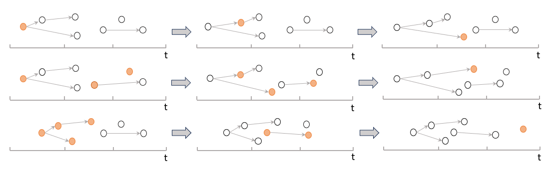
Figure 2: Illustration of different ways of updating the latent point pattern on an aggregated temporal Hawkes process with 3 temporal bins and observed data (2,3,2). We depict three methods: separate update (top row), block update by generation (middle row), and block update by cluster (bottom row). The points represent the latent times and orange points indicate the currently updated times. The arrows show the branching structure of the events.

Even though we focused on the spatio-temporal case, the method as presented applies straightforwardly to the temporal Hawkes process. We extend it to the mutually-exciting spatio-temporal Hawkes process in Section B.2.

Simulations

We investigate the performance of our method on simulated data in different scenarios. Particularly, we explore the effect that fine or coarse aggregations of time and space have on the method’s performance, and in comparison with the gold standard of fitting the Hawkes model on the exact data. We focus on the univariate temporal case in Section 4.1, the spatio-temporal case in Section 4.2, and the multivariate spatio-temporal case in Section 4.3. We present a subset of our simulations here, and we include additional simulations in Appendix E, which we summarize in Section 4.4. MCMC convergence was investigated using the Gelman-Rubin Rhat statistic, and by traceplots (shown in Appendix E).

Temporal simulations

Data for the temporal and spatio-temporal simulations were generated simultaneously, and they were aggregated in pre-defined bins. We simulate spatio-temporal data sets from a Hawkes process on a time window $[0,500]$ and a spatial window $[0,100]\times[0,100]$ using the exponential-Gaussian specification of the excitation function and parameters $\beta=\gamma=1$, and $\mu=1-\alpha$, where $\alpha\in\{0.1,0.3,0.5,0.7,0.9\}$. Data sets generated by these parameter sets have approximately 500 events on average, but the process produces fewer immigrants and more offsprings for larger values of $\alpha$. Since the branching structure $\alpha$ does not depend on an event’s location, simulated data sets from the corresponding temporal Hawkes process are acquired simply by removing the spatial information. For each parameter set, we simulate 400 data sets.

In this section, we consider estimation of the parameters of the Hawkes process based on aggregated temporal data. For our simulations, we consider time aggregations in terms of the true value of $1/\beta$, which is the expected length of time between an offspring and its parent. We consider aggregated data in bins of length $\Delta^{t}=0,0.5,0.75,1,1.25,1.5$ (times 1/$\beta$), where $\Delta^{t}=0$ indicates that there is no aggregation. We consider the performance of the proposed Bayesian method, and the frequentist MC-EM approach proposed by Shlomovich et al. (2022). For each data set, we consider the Hawkes model using the exact data as the “gold standard” approach. In reality, this approach is not applicable when the available data are aggregated. Then, we fit both methods on the aggregated data of all levels of coarseness.

Table 2: Results of the temporal simulation. The table shows the average posterior mean (“Estimate”), average 95% credible interval length (“CI length”), and coverage rate of the 95% credible interval (“Coverage”) for parameters $\mu,\alpha$ and $\beta$ of the Hawkes process, across 400 simulated data sets, for the exact data ($\Delta^{t}=0$), temporal aggregations of different sizes, and two sets of parameters. 95% credible interval is determined by the 2.5 and 97.5 quantiles of the posterior samples.

	Parameter set 1: $(\mu,\alpha,\beta)=(0.3,0.7,1)$				Parameter set 2: $(\mu,\alpha,\beta)=(0.5,0.5,1)$
	$\Delta^{t}$	Estimate	CI length	Coverage	$\Delta^{t}$	Estimate	CI length	Coverage
$\mu$	0	0.3115	0.1666	0.9450	0	0.5141	0.2421	0.9575
	0.5	0.3116	0.1669	0.9425	0.5	0.5149	0.2436	0.9625
	0.75	0.3122	0.1675	0.9450	0.75	0.5156	0.2446	0.9550
	1	0.3122	0.1679	0.9450	1	0.5166	0.2456	0.9475
	1.25	0.3128	0.1686	0.9450	1.25	0.5161	0.2473	0.9600
	1.5	0.3130	0.1690	0.9450	1.5	0.5178	0.2491	0.9449
$\alpha$	0	0.6854	0.2024	0.9375	0	0.4829	0.2442	0.9375
	0.5	0.6853	0.2029	0.9350	0.5	0.4820	0.2457	0.9500
	0.75	0.6847	0.2032	0.9375	0.75	0.4814	0.2466	0.9325
	1	0.6847	0.2036	0.9450	1	0.4802	0.2475	0.9350
	1.25	0.6840	0.2040	0.9425	1.25	0.4809	0.2493	0.9500
	1.5	0.6839	0.2046	0.9450	1.5	0.4792	0.2509	0.9273
$\beta$	0	1.0567	0.5995	0.9500	0	1.0909	0.9839	0.9575
	0.5	1.0599	0.6163	0.9550	0.5	1.1072	1.0630	0.9500
	0.75	1.0676	0.6382	0.9425	0.75	1.1238	1.1416	0.9475
	1	1.0700	0.6587	0.9550	1	1.1667	1.3206	0.9275
	1.25	1.0773	0.6884	0.9525	1.25	1.1796	1.4213	0.9350
	1.5	1.0836	0.7141	0.9325	1.5	1.2319	1.7509	0.9449

First, we investigate how results from our model that uses aggregated data compare to the results from the gold standard approach (denoted by $\Delta^{t}=0$). Table 2 shows the average estimate (posterior mean), average length of 95% credible interval, and coverage rate for each parameter under the different aggregations. For space considerations we include results for $\mu=0.3,\alpha=0.7$ (referred to as parameter set 1), and $\mu=\alpha=0.5$ (referred to as parameter sets 2) here, and results for the other parameter choices are shown in Section E.1. For all parameter sets, the estimates and credible interval lengths for $\mu$ and $\alpha$ are largely unaffected by the data’s temporal aggregation. On the other hand, the credible interval length for $\beta$ is on average wider, and the estimate of $\beta$ is on average larger for coarser temporal aggregations. The efficiency loss in estimating $\beta$ is expected for larger aggregations, since coarser temporal aggregations would result to fewer parent-offspring pairs that fall at different temporal bins. The coarseness of the temporal aggregation has a larger effect for $\beta$ under smaller values of $\alpha$. This is also expected as data sets with a smaller value of $\alpha$ contain fewer offsprings, and as a result, even fewer parent-offspring pairs in separate bins. These simulation results are in agreement with our theoretical identifiability results where we found that the information to estimate the parameters of the excitation function is in the parent-offspring pairs that are in different bins. The efficiency loss with larger temporal aggregations is alleviated in the presence of spatial information, as we illustrate in Section 4.2.

We compare the performance of our Bayesian method with the MC-EM method on the same data sets. We focus first on results from parameter set 1. In three simulated data sets, MC-EM did not converge and the corresponding estimates were removed. Figure 3 shows boxplots for the estimates of $\mu$, $\alpha$ and $\beta$ for both methods and different aggregations $\Delta^{t}$, under parameter set 1. The true parameter values are indicated by the red line. Both methods are essentially unbiased. The Monte Carlo variance for estimating $\mu$ and $\beta$ is similar for the two methods, but the Monte Carlo variability for $\alpha$ is lower based on our Bayesian method than when using the MC-EM method. The performance of the MC-EM algorithm deteriorates significantly under parameter set 2 and large aggregations. Results from MC-EM are unstable, the MC-EM method did not converge for 234 out of 400 simulated data sets, and yielded unreasonably large estimates when $\Delta^{t}=1.5$ (see Figure A.1 of the Appendix).

In our temporal simulations, the proposed Bayesian approach has accuracy gains in terms of estimation of $\alpha$, and is stable across all aggregations. Moreover, it offers a straightforward inference procedure. Coverage of 95% credible intervals was close to the nominal level for all parameters and aggregations. In contrast, the MC-EM approach does not offer a way for inference, and it is only applicable for the temporal Hawkes process. Thus, we do not use the MC-EM algorithm for the spatio-temporal simulations.

Figure 3: Boxplot for the estimates of $\mu,\alpha$ and $\beta$ using our Bayesian approach (left) and the MC-EM approach (right). The horizontal red lines indicate the true values which correspond to parameter set 1: ($\mu,\alpha,\beta$) = (0.3,0.7,1).

Spatio-temporal simulations

We aggregate the exact data using the true values of $\beta$ and $\gamma$ by $\Delta^{t}=0,0.5,1,1.5$ (times 1/$\beta$) and $\Delta^{s}=0,0.5,1,1.5$ (times $\gamma$). We summarize the findings here, and we present the full results of the spatio-temporal simulation in Section E.2. Across all aggregations over time and space and all parameter sets, the bias for parameters $\mu,\alpha$ and $\gamma$ was negligible. Estimation for $\beta$ was essentially unbiased across scenarios; the only exception being the case under $\alpha=0.1$, where even the gold standard that uses the exact data exhibits bias due to weak identifiability of the parameter. Credible intervals for the excitation parameters are wider under coarser aggregations to manifest more limited information, while coverage is above 90% throughout, even in the challenging settings with $\alpha$ small. Similar to the temporal case, the credible interval lengths with regards to estimation of $\mu$ and $\alpha$ do not change much as the aggregation in time and space becomes coarser. Figure 4 shows the mean length of 95% credible intervals for $\beta$ and $\gamma$ when data generated under parameter set 1 is aggregated in time and space with different aggregation sizes. Even though aggregation in time and space affect the credible interval lengths for both $\beta$ and $\gamma$, the credible interval lengths of $\beta$ are mainly influenced by time aggregation, while the credible interval lengths of $\gamma$ are mainly influenced by space aggregation.

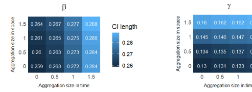
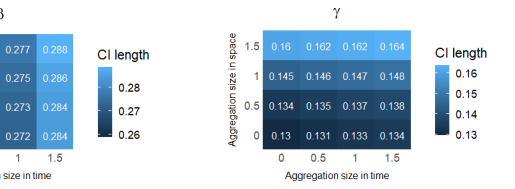
Figure 4: Average credible interval length for $\beta$ and $\gamma$ over 400 simulated spatio-temporal data sets under parameter set 1 and based on different aggregation sizes in time and space.

Lastly, we compared the results from the temporal model (Table 2 and Section E.1 and the spatio-temporal model (Section E.2). Incorporating the spatial locations leads to a reduction in bias and coverage closer to the nominal level, irrespective of the size of the time and space aggregation. In fact, the bias and efficiency loss observed for $\beta$ under large temporal aggregations in parameter set 2 is almost entirely mitigated when spatial information is available, even at coarse spatial bins. In terms of estimation efficiency, Figure 5 illustrates the CI length of the models’ common parameters $\mu$, $\alpha$, $\beta$ across the simulated data sets under parameter 1 with $\Delta^{t}=0,0.5,1,1.5$ and the coarsest space aggregation $\Delta^{s}=1.5$. Even with coarsely aggregated spatial locations, the CI lengths of all parameters are much smaller based on the spatio-temporal model than based on the temporal model. This is true even when the event times are known exactly $(\Delta^{t}=0)$. These results indicate that, if spatial information is available, incorporating it leads to more accurate estimation of the model parameters for the underlying Hawkes process, even when the location of the events is known at coarse levels. Our approach provides a framework to incorporate such coarse spatial information in the estimation procedure, and improve estimation efficiency.

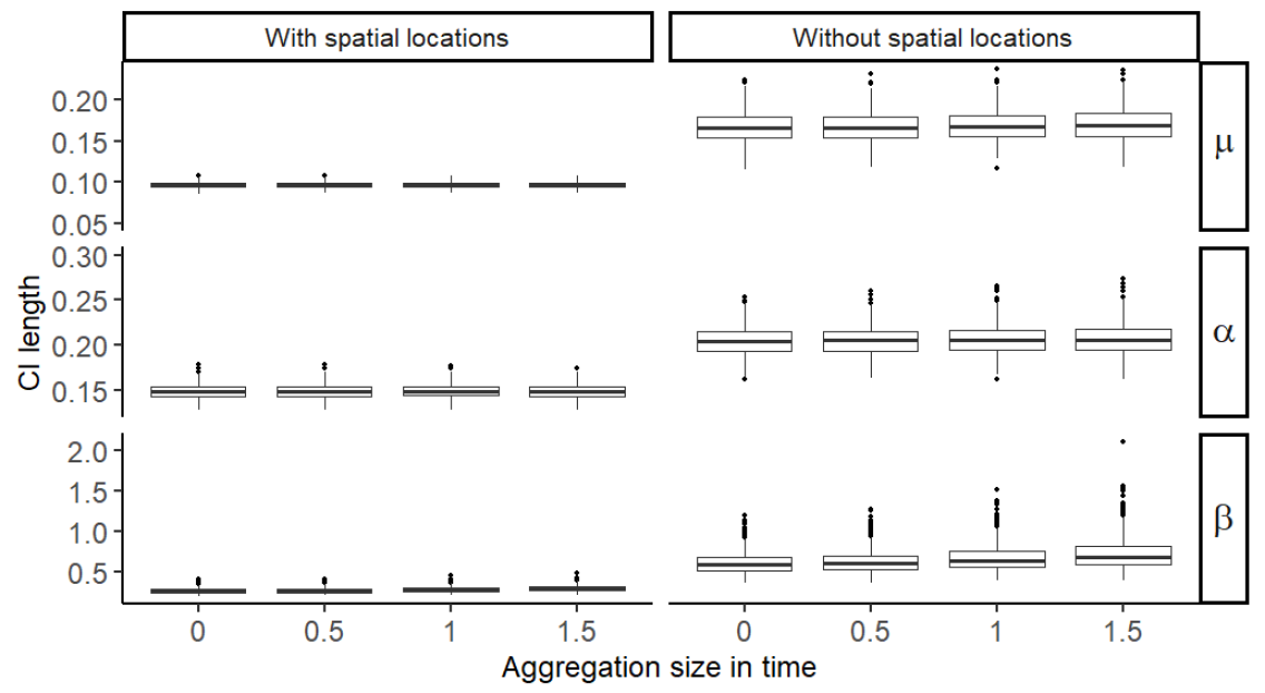
Figure 5: Credible Interval Lengths from the Temporal and Spatio-temporal Models. Boxplots of the 95% credible interval for $\mu$, $\alpha$, and $\beta$ across 400 simulated data sets under parameter set 1, for varying temporal aggregations $\Delta^{t}=0,0.5,1,1.5$ (horizontal axis) and coarse spatial aggregation $\Delta^{s}=1.5$.

Simulations on multiple spatio-temporal processes

We simulate 400 data sets from a bivariate spatio-temporal Hawkes process on the time window $[0,500]$ and the spatial window $[0,100]\times[0,100]$, using parameters

$$\mu=\begin{pmatrix}0.3\\ 0.5\end{pmatrix},\quad\alpha=\begin{pmatrix}0.7&0.15\\ 0.3&0.5\end{pmatrix},\quad\beta=\begin{pmatrix}1&1\\ 1&1\end{pmatrix},\quad\text{and}\quad\gamma=\begin{pmatrix}1&1\\ 1&1\end{pmatrix}.$$

We consider aggregations over both time and space for both processes. For ease of visualization, we aggregate data using the same coarseness for time and space, and separately for each process, i.e $\Delta_{1}^{t}=\Delta_{1}^{s}=\Delta_{1}$ and $\Delta_{2}^{t}=\Delta_{2}^{s}=\Delta_{2},$ where the subscript is used to indicate process 1 and 2. This is not necessary, and in our study of Section 5 we consider aggregations of different sizes. We consider 9 different data aggregations by varying $\Delta_{1}$ and $\Delta_{2}$ over the values 0, 0.75 and 1.

Applying our method on the aggregated data sets result in good estimates on average (Table A.9 of the Appendix). The bias for the estimated parameters is consistently low, ranging from -0.009 to 0.061, and coverage is close to nominal, varying from 92.3 to 97%, across all parameters and aggregations. Similar to the univariate case, the estimates of $\mu$ and $\alpha$ are very stable over different aggregations, with credible interval lengths that increase very slightly as the aggregations get coarser. Compared to these parameters, $\beta$ and $\gamma$ are more sensitive to coarser aggregations. Figure 6 shows the mean credible interval lengths for $\beta$ and $\gamma$ over different aggregation sizes. We find that the credible interval length for parameters that correspond to self-excitation ($\beta_{11},\beta_{22},\gamma_{11},\gamma_{22}$) are affected mostly by aggregation in the process they represent; coarser aggregation in process 1 leads to higher credible interval length for $\beta_{11},\gamma_{11}$ and little impact on the credible interval lengths for $\beta_{22},\gamma_{22}$, while the reverse is true for coarser aggregation in process 2. In contrast, parameters which correspond to external-excitation ($\beta_{12},\beta_{21},\gamma_{12},\gamma_{21}$) are similarly affected by aggregation in either process.

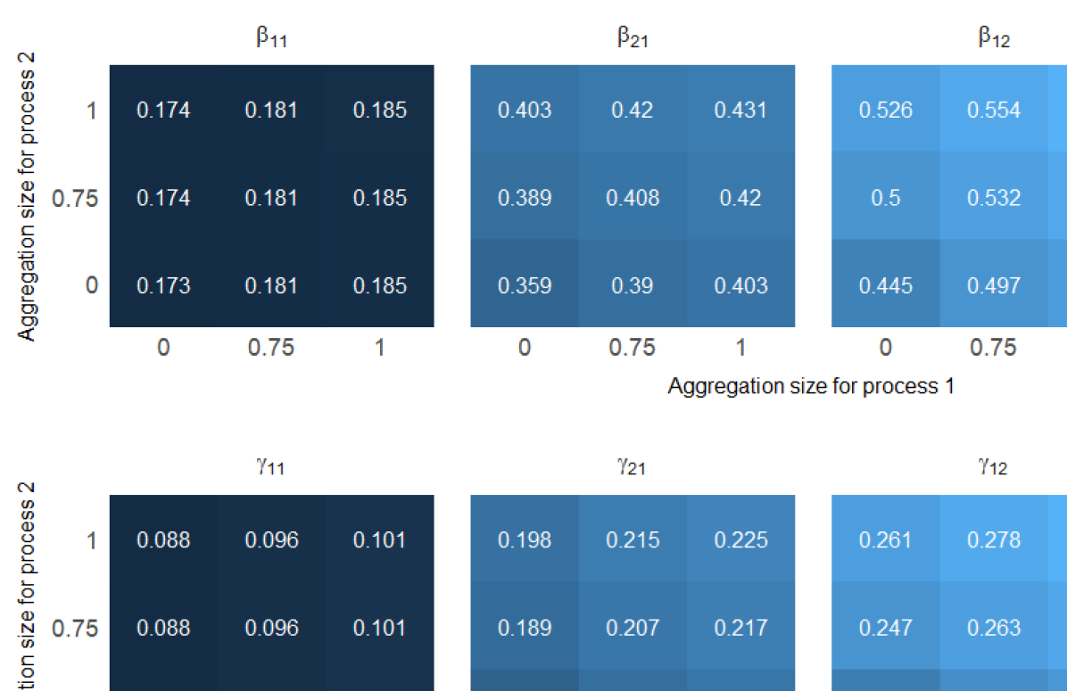
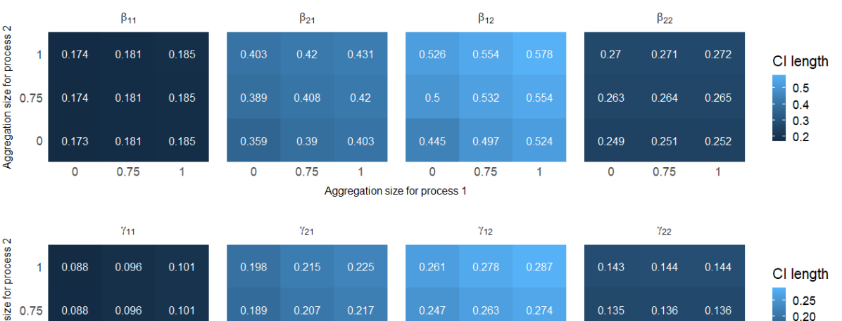
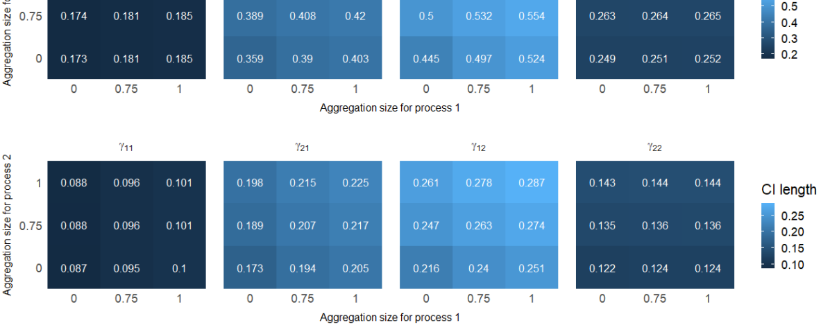
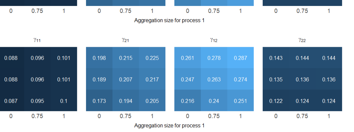
Figure 6: Average credible interval length for $\beta_{m,l}$ and $\gamma_{m,l}$ where $m,l\in\{1,2\}$ over 400 simulated multiple spatio-temporal data sets and based on different aggregation sizes in each process.

Additional simulation results

To investigate the performance of our method under alternative excitation functions, we performed simulations under the Lomax offspring kernel for the temporal component, in both temporal and spatio-temporal simulations (Section E.4). Average estimates and coverage for the parameters $\mu,\alpha$ and $\gamma$ are similar between our approach that uses aggregated data and the gold-standard that uses exact data. We find that recovering the excitation kernel is more difficult under the Lomax offspring kernel compared to the exponential offspring kernel, with coverage rate that is 89% using exact or aggregated data for the temporal simulations, and ranges between 84 and 93% for the spatio-temporal simulations.

In Section E.5 we investigated the computational time required to fit the proposed approach on temporal and spatio-temporal data. Aggregation over space or time increases computational time by 30-40% each due to the imputation of the underlying exact point pattern, in comparison to the model that uses the exact data. We find that the computational time is higher when the proportion of offspring events is higher, and that it grows linearly with the total number of events.

Application

We illustrate our method using real data of insurgent violence incidents in Iraq. Our data record time, location (latitude and longitude) and type of insurgent violence events. We focus on small arms fire (SAF) and improvised explosive device (IED) attacks from October–December 2006. We study a relatively short time period during which we could assume that the process’ dynamics are relatively constant. During the time period under study, there are 4,335 SAF attacks and 4,526 IED attacks, and the events are recorded at the minute-level with spatial resolutions at the $10^{-5}$ scale. We recognise that the available data might be subject to measurement error which we do not account for here. Instead, in the rare occasion that events are recorded to occur at exactly the same time or the same location, they are minimally jittered before any analysis by adding a draw from a uniform $\textrm{U}(0,1/120)$ (in hours) and a $\textrm{U}(0,5\times 10^{-6})$ (in degrees) distribution to the recorded time, and recorded latitude and longitude entries, respectively. We consider the resulting event timestamps and locations as the exact data for this study, and we investigate the method’s performance under coarser aggregations. The two processes are expected to have self-exciting behaviors (Lewis and Mohler, 2011), and are potentially mutually exciting. We consider temporal (Section 5.1), spatio-temporal (Section 5.2), and mutually-exciting spatio-temporal (Section 5.3) models for analyzing their behavior. We fit models on events between October 1 and December 24, using events in the last week as a holdout set.

Temporal analysis

In this section, we ignore the available spatial information and possible mutual excitement, and we fit the temporal model on SAF and IED attacks separately. We fit the model on the exact data and on aggregated data with aggregation size corresponding to $1/60,1/2,1$ and $3/2$ hours. We use a $\textrm{Gamma}(1,1)$ prior on $\beta$ that assigns a low probability on very large values of $\beta$ and small values of $1/\beta$, since we do not expect instantaneous excitement for attack events. The temporal model on the exact data for IED attacks returns a posterior mean of $\beta$ that is equal to 0.93 indicating that it takes on average 1/0.93 = 1.08 hours for an IED attack to trigger another attack. Therefore, the one and a half hour aggregation we consider is relatively coarse with respect to the process’ temporal self-excitement period.

Figure 7 shows the posterior mean and 95% credible intervals of $\mu,\alpha,\beta$ in the model fitted with exact data and aggregated data respectively, and separately for IED and SAF attacks. In both analyses, the posterior mean for $\mu,\alpha$ and $\beta$ are relatively stable across aggregation sizes. Similarly to what we observed in our simulations for aggregated temporal data (Section 4.1), the credible interval lengths for $\mu$ and $\alpha$ are almost unchanged for coarser temporal aggregations. In the IED analysis, the length of the credible interval for $\beta$ increases from 0.21 to 0.29, reflecting the uncertainty induced by the aggregation. The uncertainty in the estimate of $\beta$ is less affected in the model for the SAF attacks compared to the IED attacks. One possible reason is that the estimated $\alpha$ for SAF data is larger than that for IED data, implying that this dataset involves a higher offspring/immigrant ratio, in which case the estimation for $\beta$ is more stable across aggregation sizes as we found in our simulations (Section 4.1).

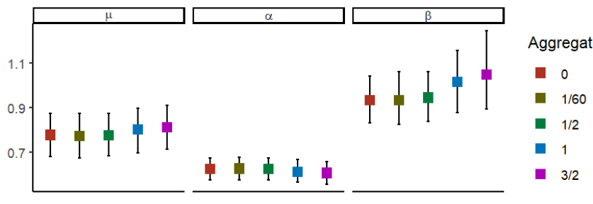
(a) IED attacks

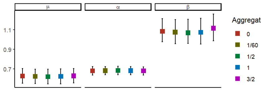
(b) SAF attacks

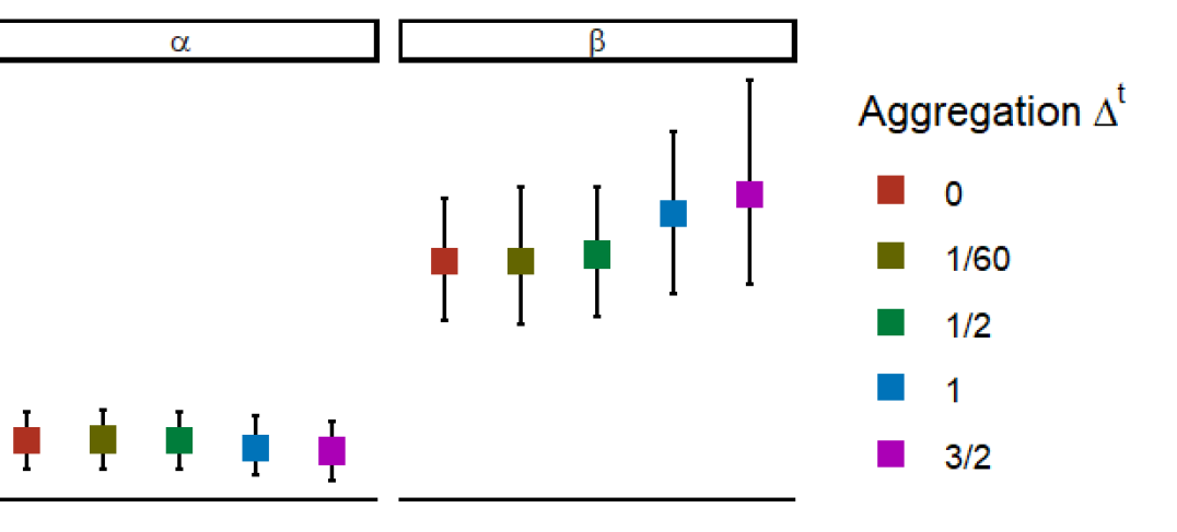
Figure 7: Posterior means and 95% credible intervals of parameters using the exact and aggregated data for IED and SAF attacks using a temporal model.

Spatio-temporal analysis

In this section, we extend the temporal analysis to include the events’ spatial information by fitting the spatio-temporal model on the SAF and IED event data separately. Figure 8 shows the location of IED and SAF attacks during our study period. The location of the events are not evenly distributed around the country, but they are mostly concentrated around Baghdad, Mosul and Al Basrah, and most of them are very close to the road network. Thus, assuming a uniform distribution for the spatial locations of the immigrants over the study area is not appropriate in this case. We modify the spatio-temporal model to specify that the location of the immigrants follows a mixture distribution:

$$f(s)=\frac{\rho}{C_{1}}\exp\Big{\{}-\frac{d^{2}_{c_{1}}(s)}{2\gamma^{2}_{c_{1}}}-\frac{d^{2}_{r}(s)}{2\gamma^{2}_{r}}\Big{\}}+\frac{1-\rho}{C_{2}}\exp\Big{\{}-\frac{d^{2}_{c_{2}}(s)}{2\gamma^{2}_{c_{2}}}-\frac{d^{2}_{r}(s)}{2\gamma^{2}_{r}}\Big{\}},$$ (8)

where $d_{r}(s)$ is the closest distance of point $s$ from the road network, $d_{c_{1}}(s)$ is the distance of point $s$ from Baghdad, and $d_{c_{2}}(s)$ is the closest distance of point $s$ from Mosul and Al Basrah. $C_{1}$ and $C_{2}$ are the normalizing constants. One could consider a 3-way mixture distribution by allowing a separate distance from Mosul and Al Basrah. However, we find that the patterns of events near those two cities are similar, and therefore we consider them simultaneously. The parameter $\rho\in(0,1)$ denotes the mixture parameter, specifying the relative prevalence of immigrants arising from the one versus the other distribution.

The prior distributions for the additional variance parameters are specified to be independent conjugate priors: $\gamma_{r}^{2}\sim\textrm{IG}(0.001,0.001),\gamma_{c_{1}}^{2}\sim\textrm{IG}(0.001,0.001),$ and $\gamma_{c_{2}}^{2}\sim\textrm{IG}(0.001,0.001),$ and the prior for $\rho$ is assumed to be $\rho\sim\textrm{Beta}(1,1).$ Sampling steps for these additional parameters are added to the procedure described in Section 3.5. Specifically, for the events labels as immigrants at each step of the MCMC, we introduce a latent variable $z\sim\textrm{Bernoulli}(\rho)$ conditional on which

$$f(s|z=1)=\frac{1}{C_{1}}\exp\Big{\{}-\frac{d^{2}_{c_{1}}(s)}{2\gamma^{2}_{c_{1}}}-\frac{d^{2}_{r}(s)}{2\gamma^{2}_{r}}\Big{\}}\quad\textrm{and}$$

$$f(s|z=0)=\frac{1}{C_{2}}\exp\Big{\{}-\frac{d^{2}_{c_{2}}(s)}{2\gamma^{2}_{c_{2}}}-\frac{d^{2}_{r}(s)}{2\gamma^{2}_{r}}\Big{\}}.$$

Note that we only need latent variable $z$ for immigrants, and additional parameters are $(\gamma_{r},\gamma_{c_{1}},\gamma_{c_{2}},\bm{z})$, where $\bm{z}=\{z_{i}:i\in I\}$. Then the conditional posteriors for these parameters are:

$$z_{i}|\mathbf{N},\bm{x},\bm{Y},\theta,\rho\sim\textrm{Bernoulli}\Big{(}\frac{\rho f(s_{i}|z_{i}=1)}{\rho f(s_{i}|z_{i}=1)+(1-\rho)f(s_{i}|z_{i}=0)}\Big{)}$$

$$\gamma_{r}^{2}|\mathbf{N},\bm{x},\bm{Y},\bm{z}\sim\textrm{IG}\Big{(}0.001+|I|,0.001+\frac{1}{2}\sum_{i\in I}d^{2}_{r}(s_{i})\Big{)}$$

$$\gamma_{c_{1}}|\mathbf{N},\bm{x},\bm{Y},\bm{z}\sim\textrm{IG}\Big{(}0.001+\sum_{i\in I}1{\{z_{i}=1\}},0.001+\frac{1}{2}\sum_{i\in I}d^{2}_{c_{1}}(s_{i})\Big{)}$$

$$\gamma_{c_{2}}|\mathbf{N},\bm{x},\bm{Y},\bm{z}\sim\textrm{IG}\Big{(}0.001+\sum_{i\in I}1{\{z_{i}=0\}},0.001+\frac{1}{2}\sum_{i\in I}d^{2}_{c_{2}}(s_{i})\Big{)},\quad\text{and}$$

$$\rho|\mathbf{N},\bm{x},\bm{Y},\bm{z}\sim\mathrm{Beta}\Big{(}1+\sum_{i\in I}1{\{z_{i}=1\}},1+\sum_{i\in I}1{\{z_{i}=0\}}\Big{)}.$$

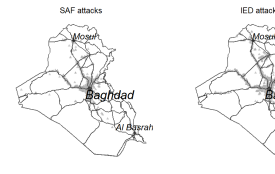
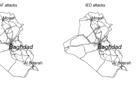
Figure 8: Locations of SAF and IED attacks in Iraq from October-December 2006. Attacks are mostly concentrated near the three cities and the main road network.

We examine the performance of our method based on different coarseness of aggregation. Using the exact data, we find that the posterior mean of $\beta$ is approximately $0.01$ for both processes, meaning that it takes on average about $100$ hours for an event to trigger another event when spatial information is incorporated. Therefore, we consider hourly and daily temporal aggregations, i.e $\Delta^{t}=1,24$ (hours), as these aggregations are commonly seen in practice. We also find that, based on the exact data, the estimates of the location parameters ($\gamma,\gamma_{r},\gamma_{c_{1}},\gamma_{c_{2}}$) in the spatial distribution are equal to (0.0054, 0.062, 1.04, 0.09) for SAF attacks and (0.0046, 0.063, 1.31, 0.087) for IED attacks. Approximately, 1 degrees is equal to 111 kilometers, so these estimates correspond to about (0.6, 6.9, 115.4, 10) and (0.5, 7, 145, 9.7) kilometers, respectively. Based on the smallest value, we choose to aggregate the space with $\Delta^{s}\in\{0.001,0.005\}$, corresponding to a little over 100 meters, and 0.5 kilometer.

Figure 9 shows the posterior mean and 95% intervals of all parameters in the spatio-temporal Hawkes process ($\mu$,$\alpha$,$\beta$,$\gamma$,$\gamma_{r}$,$\gamma_{c_{1}}$,$\gamma_{c_{2}}$,$\rho$) using exact and aggregated data for IED and SAF attacks separately. Focusing on the results for the SAF attacks in Figure 9b, we find that for a fixed value of $\Delta^{s}$, results on all these parameters are comparable across temporal aggregations: the posterior means remain nearly the same and the credible interval length increases very little as $\Delta^{t}$ increase. The impact of coarser spatial aggregations (larger values of $\Delta^{s}$) on estimated parameters is more prevalent. We focus first on the posterior distribution for the parameters in the distribution of the immigrant locations ($\gamma_{r}$, $\gamma_{c_{1}}$, $\gamma_{c_{2}}$, $\rho$). We find that the posterior mean for these parameters is similar across spatial aggregations. The corresponding credible interval lengths increase slightly for larger values of $\Delta^{s}$, with percentage change in the credible interval length ranging from 2.31% to 8.82% for the coarsest aggregation size considered. When investigating the posterior distribution of $\mu$, $\alpha$, $\beta$, and $\gamma$, we find that the posterior mean changes significantly for the coarsest spatial aggregation ($\Delta^{s}=0.005.$) Possible reasons are that the number of events in some space grid is large and we may not have enough information to learn the true parameters, or that the multivariate normal distribution may not accurately capture the distribution of the offspring locations given the fact that many events occurs at nearly the same place. We do the same analysis on the IED data and get comparable result shown in Figure 9a.

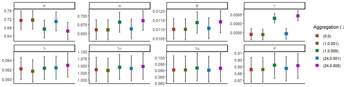
(a) IED attacks

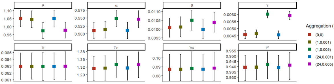
(b) SAF attacks

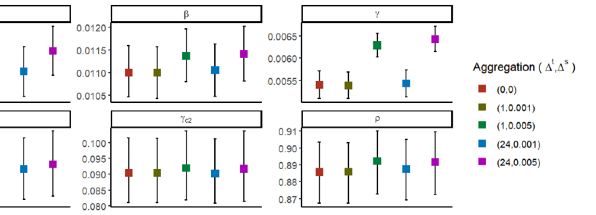
Figure 9: Posterior means and 95% credible intervals of parameters using exact and aggregated spatio-temporal data.

Mutually exciting process analysis

Finally, we model IED and SAF data allowing for mutual excitement. We consider aggregated SAF and IED data using the same aggregation size in time and space as in Section 5.2, i.e. $\Delta^{t}_{1}=\Delta^{t}_{2}\in\{1,24\}$ and $\Delta^{s}_{1}=\Delta^{s}_{2}\in\{0.001,0.005\}$. We maintain the distribution of immigrant locations in Equation 8, and we specify the same priors for the additional, cross-excitement parameters. Figure 10 shows the posterior mean and 95% for all parameters over different aggregation. We note that estimates of $\mu$ and $\alpha$ for the self-excitation ($\mu_{1},\mu_{2},\alpha_{11},\alpha_{22}$) are smaller than the corresponding estimates from the separate spatio-temporal models in Section 5.2. This occurs because some events that were previously labeled as immigrants or offsprings due to self-excitation are now labeled offsprings due to external-excitation. Moreover, the effects of aggregation on those parameters are similar to that on corresponding parameters in Section 5.2. For example, we can see the changes in $\beta_{22}$ estimate is comparable to $\beta$ estimate shown in Figure 9b. For $\beta$ and $\gamma$, the posterior means of external-excitation parameters ($\beta_{12},\beta_{21},\gamma_{12},\gamma_{21}$) are more sensitive to the aggregation in space compare to self-excitation parameters ($\beta_{11},\beta_{22},\gamma_{11},\gamma_{22}$). More specifically, the credible interval lengths of $\beta_{12}$ and $\beta_{21}$ range from 0.0011 to 0.0014, and the credible interval lengths of $\beta_{11}$ and $\beta_{22}$ range from 0.0029 to 0.0033 across all aggregations considered.

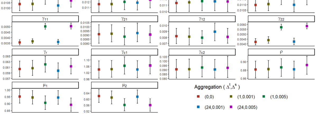
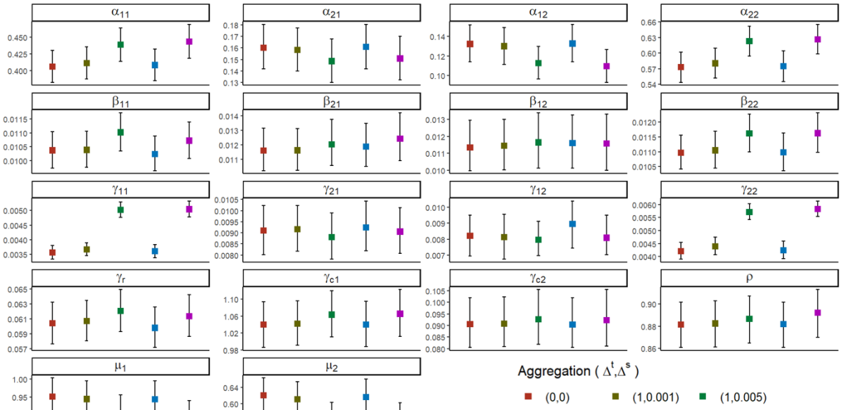
Figure 10: Posterior means and 95% credible intervals of parameters from the mutually-exciting Hawkes process using exact and aggregated spatio-temporal data. Process 1: IED, process 2: SAF.

Prediction

We also examined the temporal, spatio-temporal, and multivariate spatio-temporal models’ forecasting ability, as well as the effects of aggregation on the models’ forecasts. We used the predictive posterior distribution for forecasting events in the holdout set, defined as $p(\tilde{\bm{x}}|\bm{N})=\int p(\tilde{\bm{x}}|\theta,\bm{x})p(\bm{x},\theta|\bm{N})\,\text{d}\bm{x}\,\text{d}\theta,$ where $\tilde{\bm{x}}$ is the predicted data, $\bm{N}$ is the observed data and $\bm{x}$ is the corresponding latent exact point pattern. We draw forecasts $\tilde{\bm{x}}$ by iteratively sampling the parameters $\theta$ and the latent point pattern $\bm{x}$ from their posterior distribution, and imputing $\tilde{\bm{x}}$ from $p(\tilde{\bm{x}}|\theta,\bm{x})$ using Algorithm 1 in Tucker et al. (2019). Then, we forecast the number of events in a certain time period or region (if spatial location is available), by counting the number of predicted events that fall in that window.

For the temporal analysis, we evaluate the posterior prediction for the number of attacks in the following day and the following week. For the spatio-temporal analyses, we consider the number of events in the following week in five selected regions around cities in Iraq. We compare our forecasts to the observed data. The results are shown in Appendix G. We find that all models predict the total number of SAF and IED attacks in the country accurately, and forecasts based on the exact data and the coarsest aggregation are essentially indistinguishable. The spatio-temporal models perform relatively well in forecasting the number of events in the different regions of Iraq, except they over-estimate the number of attacks in the region between Baghdad and Al Basrah, which might be due to misspecification of the excitation kernel.

We also estimated the intensity of events in the holdout time period by applying kernel density estimation to the posterior predictive samples from the models using the exact data and the coarsest aggregation. In Figure 11 we show the log of the mean of estimated intensities for SAF attacks based on the multivariate spatio-temporal model for the exact and the aggregated data. We find that the posterior predictive distributions are consistent across aggregations. We see that the observed attacks (depicted with round points) occur at the areas of highest estimated intensity, illustrating that the model forecasts agree with what actually occurred. In Appendix G, we also see that they are consistent across the spatio-temporal models.

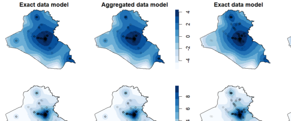
Figure 11: Logarithm of the mean intensity for forecasting SAF attacks in the last week of 2006 based on the exact data (left) and aggregated data with $\Delta^{t}=24$ and $\Delta^{s}=0.005$ (right). The black points show the true attack locations. The intensity is estimated based on the posterior predictive samples in the mutually exciting model.

Discussion

In this paper, we proposed a Bayesian estimation procedure for aggregated Hawkes processes. We handle the aggregation by treating the exact data as latent variables updated by an extra step in the MCMC algorithm for exact Hawkes processes. We examine the effect of aggregation sizes in time and space, and find consistent results. Compared with a frequentist method for aggregated temporal Hawkes processes (Shlomovich et al., 2022), our method achieves comparable or lower bias on simulated data, and provides a straightforward way to perform inference and incorporate spatial information. Our method is applicable for temporal and spatio-temporal point pattern data, and data on multiple processes. We analyze real data on insurgent violence attacks in Iraq and find consistent results across different aggregation sizes.

Additional work on aggregated point pattern data can extend in various directions. Firstly, one issue that was ignored is the potential edge effects in time and space. Events that happen outside the observed temporal and spatial window can affect parameter estimates. Edge correction methods for exact data are discussed in Lapham (2014), Diggle (2013) and Cronie and Särkkä (2011), and implementing them for aggregated point processes can be explored in future work. Secondly, an interesting extension of our work could target marked Hawkes processes where features of events are available and might drive the process dynamics. For example, in our study of Section 5, the number of civilian casualties caused by an attack, if available, can be included as a mark in the model. In such cases, one might want to allow an event’s number of offsprings $\alpha$ to depend on the mark, since the number of casualties caused by an attack may affect the number of attacks it can incite. Doing so would be of explicit interest and it could complicate estimation. Thirdly, it would be interesting to investigate nonparametric Hawkes process models in the presence of aggregated point pattern data, which are used in many applications for extra flexibility. For instance, Lewis and Mohler (2011), Fox et al. (2016) and Marsan and Lengline (2008) introduce ways to incorporate nonparametric inhomogeneous $\mu(t)$, and Zhou et al. (2013) and Kirchner and Bercher (2018) use kernel density estimation for the offspring intensity. Moreover, the multivariate Hawkes process has been extended to allow for inhibition effects within a Bayesian estimation procedure (Deutsch and Ross, 2022), which can be explored within the realm of aggregated data as well. Lastly, it is of interest to us to investigate the implications of using aggregated point pattern data for learning causal dependencies among processes (Papadogeorgou et al., 2022), especially when these effects might manifest almost instantaneously in time.

Supplementary Appendix for “Bayesian inference for aggregated Hawkes processes”

Appendix A Table of notation

Definitions for the notation used in the manuscript are given in Table A.1.

Table A.1: Notation

$X=\{(t_{i},s_{i})\}$	A spatio-temporal process
$\theta$	Parameter vector for marked Hawkes process
$\bm{Y}$	Branching structure
$I$	Collection of all immigrants
$O$	Collection of all offspring
$O_{j}$	Collection of all offspring of events $j$
$\alpha$	Total offspring intensity
$g(t,s)$	Normalized offspring intensity
$\Delta^{t}$	Aggregation size in time
$\Delta^{s}$	Aggregation size in space
$B^{t}_{i}$	$i^{th}$ Time bins
$B^{s}_{i}$	$i^{th}$ Space bins
$N_{i,j}$	Number of events in $B^{t}_{i}\times B^{s}_{j}$

Appendix B Multivariate Hawkes processes

In this section, we provide details on the model formulation and estimation technique for multivaraite HPs. In Section B.1, we discuss how to formulate the model for the aggregated multivariate HP using latent variables for the exact data. Then, in Section B.2, we discuss prior choice and MCMC for the multivariate HP under the exponential and Gaussian specification for the offspring densities.

Latent variable formulation for multivariate Hawkes processes

Suppose we observe $L$ aggregated Hawkes processes on $[0,T]\times W$. Assuming the same notations in Section 3.1 of the manuscript, the observed data is $\bm{N}=\{N_{l,i,j}:l=1,\dots,L,i=1,\dots,n_{l,1},j=1,\dots,n_{l,2}\}$. Let $x=\{(t_{l,i},s_{l,i}):l=1,\dots,L,i=1,\dots,n_{l}\}$ be the underlying exact data which is unobserved, and $\bm{Y}=\{Y_{l,i}:l=1,\dots,L,i=1,\dots,n_{l}\}$ be the latent branching structure. The parameters for the continuous Hawkes process are now $\theta=(\mu,\alpha,\beta,\gamma)$, where $\mu=(\mu_{l}:l=1,\dots,L)$, $\alpha=(\alpha_{m,l}:m,l=1,\dots,L)$, $\beta=(\beta_{m,l}:m,l=1,\dots,L)$, $\gamma=(\gamma_{m,l}:m,l=1,\dots,L)$. In this case, the distribution of aggregated data $p(\bm{N}|\bm{x},\bm{Y},\theta)$ is equal to 1 only when the aggregated aggregated data agrees the exact data for each process: $\sum_{i=1}^{n_{1}}\sum_{j=1}^{n_{2}}N_{i,j}=n_{l}$ and $\sum_{k=1}^{n_{l}}=1{\{(t_{l,k},s_{l,k})\in B_{l,i}^{t}\times B_{l,j}^{s}\}}=N_{l,i,j}$ for all $i,j,l$. Similar to Section 3.2 of the manuscript, we need to sample from $p(\bm{x}|\bm{Y},\theta)$ and $p(\theta,\bm{Y}|\bm{x})$ iteratively.

Estimation and inference for multivariate Hawkes processes within the Bayesian framework

The MCMC sampling scheme discussed below corresponds to the formulation where exponential and Gaussian densities are chosen for the temporal and spatial components of the excitation function, respectively, for all components of the multivariate HP.

Prior distributions

For $m,l\in\{1,\dots,L\}$, we assume (independent) gamma priors for $\mu_{l}$, $\alpha_{m,l}$ and $\beta_{m,l}$, and inverse gamma priors for $\gamma^{2}_{m,l}$:

$$\mu_{l}\sim\textrm{Gamma}(a_{l,1},b_{l,1}), \alpha_{m,l}\sim\text{Trunc}\textrm{Gamma}(a_{m,l,2},b_{m,l,2}),\,$$

$$\beta_{m,l}\sim\textrm{Gamma}(a_{m,l,3},b_{m,l,3}), \gamma_{m,l}^{2}\sim\textrm{IG}(a_{m,l,4},b_{m,l,4}).$$

Conditional distribution of latent exact data

Given the latent branching structure and model parameters, the distribution of exact data (under the exponential-Gaussian specification of the excitation function) is

$$p(\bm{x}|\bm{Y},\theta) =\prod_{l=1}^{L}\exp(-\mu_{l}T)(\mu_{l}|W|^{-1})^{|I_{l}|}$$

$$\hskip 10.0pt\times\prod_{m=1}^{L}\prod_{i=1}^{n_{m}}\prod_{l=1}^{L}\Big{\{}\exp\big{\{}-\alpha_{m,l}\{1-\exp[-\beta_{m,l}(T-t_{m,i})]\}\big{\}}$$

$$\hskip 10.0pt\times\prod_{t_{l,j}\in O_{m,i}}\frac{\alpha_{m,l}\beta_{m,l}}{\sqrt{2\pi\gamma_{m,l}^{2}}}\exp\Big{[}-\beta_{m,l}(t_{l,j}-t_{m,i})-\frac{\|s_{l,j}-s_{m,i}\|^{2}}{2\gamma_{m,l}^{2}}\Big{]}\Big{\}},$$

where $I_{l}$ denotes the set of immigrants in process $l$ and $O_{m,i}$ denotes the set of offsprings of event $i$ in process $m$.

MCMC updates

We use Gibbs sampling for each of the parameter in $\theta$ and the latent branching structure $\bm{Y}$. Specifically, we iteratively sample from the parameters according to the distributions below:

$$\mu_{l}|\bm{x},\theta_{-\mu_{l}},\bm{Y},\bm{N} \sim\textrm{Gamma}\big{(}a_{l,1}+|I_{l}|,b_{l,1}+T\big{)}$$

$$\alpha_{m,l}|\bm{x},\theta_{-\alpha_{m,l}},\bm{Y},\bm{N} \sim\textrm{Gamma}\big{(}a_{m,l,2}+\sum_{i=1}^{n_{m}}|O_{m,i}|,$$

$$\hskip 60.0ptb_{m,l,2}+\sum_{i=1}^{n_{m}}\beta_{m,l}\exp(-\beta_{m,l}(T-t_{m,i}))\big{)}$$

$$\gamma^{2}_{m,l}|\bm{x},\theta_{-\gamma_{m,l}},\bm{Y},\bm{N} \sim\textrm{IG}\big{(}a_{m,l,4}+\sum_{i=1}^{n_{m}}|O_{m,i}|,$$

$$\hskip 60.0ptb_{m,l,4}+\frac{1}{2}\sum_{i=1}^{n_{m}}\sum_{t_{l,j}\in O_{m,i}}\|s_{l,j}-s_{m,i}\|^{2}\big{)}.$$

We sample $Y_{l,i}$ from its full conditional distribution which is a multinomial distribution given by

$$P(Y_{l,i}=(m,j)\mid\theta,\bm{x},\bm{N})\propto\begin{cases}\mu_{l}|W|^{-1},\\ \hskip 60.0pt\text{for }m=j=0,\quad\text{and}\\[5.0pt] \dfrac{\alpha_{m,l}\beta_{m,l}}{\sqrt{2\pi\gamma_{m,l}^{2}}}\exp(-\beta_{m,l}(t_{l,i}-t_{m,j})-\frac{\|s_{l,i}-s_{m,j}\|^{2}}{2\gamma_{m,l}^{2}}),\\ \hskip 60.0pt\text{for }m>0,j>0,t_{m,k}<t_{l,i}\end{cases}$$

Let $\bm{t},\bm{s}$ denote vectors of the exact time and spatial marks of all events respectively. Since there are no conjugate priors for $\bm{t},\bm{s}$ and $\beta_{m,l}$, we use element-wise Metropolis-Hasting to sample from their full conditionals. Specifically, we propose value $\beta_{m,l}^{\prime}$ from a normal distribution with mean $\beta_{m,l}^{c}$ and standard deviation $\sigma_{\beta_{m,l}}$. We accept the move with probability

$$H_{\beta_{m,l}} =\min\Big{(}1,\Big{(}\frac{\beta_{m,l}^{\prime}}{\beta_{m,l}^{c}}\Big{)}^{a_{m,l,3}-1}\exp(b_{m,l,3}(\beta_{m,l}^{c}-\beta_{m,l}^{\prime}))$$

$$\hskip 50.0pt\times\prod_{i=1}^{n_{m}}\Big{\{}\exp\Big{(}\alpha_{m,l}\exp(-\beta_{m,l}^{\prime}(T-t_{m,i}))-\alpha_{m,l}\exp(-\beta_{m,l}^{c}(T-t_{m,i}))\Big{)}$$

$$\hskip 50.0pt\times\prod_{j\in O_{m,i}}\frac{\beta_{m,l}^{\prime}}{\beta_{m,l}^{c}}\exp\Big{(}-(\beta_{m,l}^{\prime}-\beta_{m,l}^{c})(t_{l,j}-t_{m,i})\Big{)}\Big{\}}\Big{)}$$

For $i=1,2\dots,n_{m}$, $t_{m,i}^{\prime}$ is drawn from a continuous uniform distribution that satisfies the following restrictions: $t_{m,i}^{\prime}$ is within the time bin of event $i$ in process $m$, it occurs after its parent event (if it has one, $Y_{m,i}\neq(0,0)$), and before its offsprings (if any). The proposed value of $t_{m,i}$ is accepted with probability

$$H_{t_{m,i}}=\min\Big{(}1, \exp\Big{(}\alpha_{m,l}\beta_{m,l}\exp(-\beta_{m,l}(T-t_{m,i}^{c}))-\alpha_{m,l}\beta_{m,l}\exp(-\beta_{m,l}(T-t_{m,i}^{\prime})))$$

$$-(|O_{m,i}|+1{\{Y_{m,i}\neq(0,0)\}})\beta_{m,l}(t_{m,i}^{\prime}-t_{m,i}^{c})\Big{)}\Big{)}.$$

Similarly, $s_{m,i}$ is drawn from a uniform distribution on the space bin containing $s_{m,i}$ and the proposed move is accepted with probability

$$H_{s_{m,i}}=\min\Big{(}1,\ \exp\Big{(}\frac{-\|s_{m,i}^{\prime}-s_{\textrm{pa}}\|^{2}+\|s_{m,i}^{c}-s_{\textrm{pa}}\|^{2}}{2\gamma_{q,l}^{2}}1{\{Y_{m,i}\neq(0,0)\}}+$$

$$\hskip 90.0pt+\sum_{j\in O_{m,i}}\frac{-\|s_{m,i}^{\prime}-s_{l,j}\|^{2}+\|s_{m,i}^{c}-s_{l,j}\|^{2}}{2\gamma_{m,l}^{2}}\Big{)}\Big{)},$$

where $q$ is the process that contains the parent of $t_{m,i}.$

Appendix C Theoretical Proofs of Identifiability

Identifiability for aggregated temporal models

In order to prove Theorem 3.1, let us first show a more general identifiability result for aggregated temporal models.

Theorem C.1 (Identifiability for temporal models).

Let $\{t_{1},\dots,t_{n}\}$ be a temporal Hawkes process on $[0,T)$ defined by intensity $\lambda_{\theta}^{*}(t)=\mu+\sum_{t_{i}<t}\alpha g(t-t_{i}),$ where $\theta$ is the vector containing $\mu,\alpha$ and parameters in $g(t)$. Let $\bm{B}=\{B_{1},\dots,B_{k}\}$ be temporal bins with equal bin length $\Delta$ and $\bm{N}=\{N_{1},N_{2},\dots,N_{k}\}$ be the corresponding aggregated temporal Hawkes process. Let $h_{\theta}(t)=\int_{0}^{t}\alpha g(u)\,\text{d}u$. Suppose that $h_{\theta_{1}}(t)-h_{\theta_{2}}(t)$ has at most $k-1$ roots on $(0,T)$ whenever $h_{\theta_{1}}\neq h_{\theta_{2}}$. If $P_{\theta_{1}}(N_{1}=n_{1},\dots,N_{k}=n_{k})=P_{\theta_{2}}(N_{1}=n_{1},\dots,N_{k}=n_{k})$ for all $(n_{1},\dots,n_{k})\in\mathbb{N}^{k}$, then $\theta_{1}=\theta_{2}$.

Proof.

We follow proof by contradiction. Suppose that there exist $\theta_{1}\neq\theta_{2}$ such that $P_{\theta_{1}}(N_{1}=n_{1},\dots,N_{k}=n_{k})=P_{\theta_{2}}(N_{1}=n_{1},\dots,N_{k}=n_{k})$ for all $(n_{1},\dots,n_{k})\in\mathbb{N}^{k}.$ Since

$$P_{\theta}(N_{1}=0)=e^{-\mu\Delta},$$

we have

$$P_{\theta_{1}}(N_{1}=0)=e^{-\mu_{1}\Delta}=e^{-\mu_{2}\Delta}=P_{\theta_{2}}(N_{1}=0).$$

So $\mu_{1}=\mu_{2},$ and thus $h_{\theta_{1}}\neq h_{\theta_{2}}.$ By assumption, there exist $i\in\{1,\dots,k\}$ such that $B_{i}$ does not contain zeros of $h_{\theta_{1}}(t)-h_{\theta_{2}}(t)$. WLOG, suppose $h_{\theta_{1}}(t)>h_{\theta_{2}}(t)$ for $t\in B_{i}=[(i-1)\Delta,i\Delta).$ Then

$$\int_{(i-1)\Delta}^{i\Delta}\exp\big{(}-h_{\theta_{1}}(x)\big{)}\,\text{d}x<\int_{(i-1)\Delta}^{i\Delta}\exp\big{(}-h_{\theta_{2}}(x)\big{)}\,\text{d}x$$

Note that

$$P_{\theta}(N_{1}=1,N_{2}=0,\dots,N_{i-1}=0,N_{i}=0)$$

$$= \int_{0}^{\Delta}\lambda^{*}(t_{1})\exp\Big{(}\int_{0}^{i\Delta}\lambda^{*}(t)\,\text{d}t\Big{)}\,\text{d}t_{1}$$

$$= \int_{0}^{\Delta}\mu e^{-\mu i\Delta}\exp\big{(}-h_{\theta}(i\Delta-t_{1})\big{)}\,\text{d}t_{1}$$

$$= \int_{(i-1)\Delta}^{i\Delta}\mu e^{-\mu i\Delta}\exp\big{(}-h_{\theta}(x)\big{)}\,\text{d}x$$

Thus,

$$P_{\theta_{1}}(N_{1}=1,N_{2}=0,\dots,N_{i-1}=0,N_{i}=0)$$

$$\hskip 20.0pt<P_{\theta_{2}}(N_{1}=1,N_{2}=0,\dots,N_{i-1}=0,N_{i}=0),$$

a contradiction.

∎

Lemma C.2 (Properties of exponential offspring kernel).

Let $h_{\theta}(t)=\alpha(1-e^{-\beta t})$ where $\theta=(\alpha,\beta)\in(0,1)\times(0,\infty).$ If $\theta_{1}\neq\theta_{2}$, then $h_{\theta_{1}}-h_{\theta_{2}}$ has at most 1 root on $(0,\infty).$

Proof.

By contradiction, there exists $\theta_{1}\neq\theta_{2}$ such that $h_{\theta_{1}}(t)-h_{\theta_{2}}(t)$ has st least two positive roots. Since $h_{\theta_{1}}(0)-h_{\theta_{2}}(0)=0$, the derivative $h_{\theta_{1}}^{\prime}(t)-h_{\theta_{2}}^{\prime}(t)$ changes sign at least twice on $(0,\infty).$ Note that

$$\frac{h_{\theta_{1}}^{\prime}(t)}{h_{\theta_{2}}^{\prime}(t)}=\frac{\alpha_{1}\beta_{1}}{\alpha_{2}\beta_{2}}e^{(\beta_{2}-\beta_{1})t}$$

is a monotonic function for $t\in(0,\infty).$ So $h_{\theta_{1}}^{\prime}(t)-h_{\theta_{2}}^{\prime}(t)$ is also monotone on $(0,\infty).$ Thus, $h_{\theta_{1}}^{\prime}(t)-h_{\theta_{2}}^{\prime}(t)$ changes sign at most once, which leads to a contradiction. Hence, $h_{\theta_{1}}-h_{\theta_{2}}$ has at most 1 root on $(0,\infty).$ ∎

Lemma C.3 (Properties of Lomax offspring kernel).

Let $h_{\theta}(t)=\alpha-\alpha\Big{(}\frac{c}{c+x}\Big{)}^{p-1}$ where $\theta=(\alpha,c,p)\in(0,1)\times(0,\infty)\times(1,\infty).$ If $\theta_{1}\neq\theta_{2}$, then $h_{\theta_{1}}-h_{\theta_{2}}$ has at most 2 roots on $(0,\infty).$

Proof.

By contradiction, there exists $\theta_{1}\neq\theta_{2}$ such that $h_{\theta_{1}}(t)-h_{\theta_{2}}(t)$ has at least three positive roots. Since $h_{\theta_{1}}(0)-h_{\theta_{2}}(0)=0$, the derivative $h_{\theta_{1}}^{\prime}(t)-h_{\theta_{2}}^{\prime}(t)$ changes sign at least three times on $(0,\infty).$ Observe that $h_{\theta_{1}}^{\prime}(t)-h_{\theta_{2}}^{\prime}(t)$ and $\log h^{\prime}_{\theta_{1}}(t)-\log h^{\prime}_{\theta_{2}}(t)$ have the same sign. So the function $\log h^{\prime}_{\theta_{1}}(t)-\log h^{\prime}_{\theta_{2}}(t)$ changes sign at least three times on $(0,\infty).$ Note that

$$\frac{d}{dt}\Big{(}\log h^{\prime}_{\theta_{1}}(t)-\log h^{\prime}_{\theta_{2}}(t)\Big{)}=\frac{\alpha_{1}p_{1}}{c_{1}+x}-\frac{\alpha_{2}p_{2}}{c_{2}+x}.$$

We have the following three cases:

Case 1.

Suppose $\alpha_{1}p_{1}=\alpha_{2}p_{2}$ and $c_{1}=c_{2}$. Then $\frac{d}{dt}\Big{(}\log h^{\prime}_{\theta_{1}}(t)-\log h^{\prime}_{\theta_{2}}(t)\Big{)}=0$ for all $t\in(0,\infty).$ So $\log h^{\prime}_{\theta_{1}}(t)-\log h^{\prime}_{\theta_{2}}(t)$ is constant. So $\log h^{\prime}_{\theta_{1}}(t)-\log h^{\prime}_{\theta_{2}}(t)$ does not change sign on $(0,\infty)$, a contradiction.

Case 2.

Suppose $\alpha_{1}p_{1}=\alpha_{2}p_{2}$ and $c_{1}\neq c_{2}$. WLOG, assume $c_{1}<c_{2}.$ Then $\frac{d}{dt}\Big{(}\log h^{\prime}_{\theta_{1}}(t)-\log h^{\prime}_{\theta_{2}}(t)\Big{)}>0$ for $t\in(0,\infty).$ So $\log h^{\prime}_{\theta_{1}}(t)-\log h^{\prime}_{\theta_{2}}(t)$ is increasing on $(0,\infty)$. Thus, $\log h^{\prime}_{\theta_{1}}(t)-\log h^{\prime}_{\theta_{2}}(t)$ changes sign at most once on $(0,\infty)$, a contradiction.

Case 3.

Suppose $\alpha_{1}p_{1}\neq\alpha_{2}p_{2}$. Then $t_{0}=\frac{\alpha_{1}p_{1}c_{2}-\alpha_{2}p_{2}c_{1}}{\alpha_{2}p_{2}-\alpha_{1}p_{1}}$ is the unique solution for $\frac{d}{dt}\Big{(}\log h^{\prime}_{\theta_{1}}(t)-\log h^{\prime}_{\theta_{2}}(t)\Big{)}=0$, and the function $\frac{d}{dt}\Big{(}\log h^{\prime}_{\theta_{1}}(t)-\log h^{\prime}_{\theta_{2}}(t)\Big{)}$ changes sign at $t_{0}.$ WLOG, suppose $\frac{d}{dt}\Big{(}\log h^{\prime}_{\theta_{1}}(t)-\log h^{\prime}_{\theta_{2}}(t)\Big{)}<0$ for $t<t_{0}$ and $\frac{d}{dt}\Big{(}\log h^{\prime}_{\theta_{1}}(t)-\log h^{\prime}_{\theta_{2}}(t)\Big{)}>0$ for $t>t_{0}.$ Then $\log h^{\prime}_{\theta_{1}}(t)-\log h^{\prime}_{\theta_{2}}(t)$ is decreasing for $t<t_{0}$ and increasing for $t>t_{0}.$ Thus, $\log h^{\prime}_{\theta_{1}}(t)-\log h^{\prime}_{\theta_{2}}(t)$ changes sign at most twice on $(-\infty,\infty)$, a contradiction.

∎

Proof of Theorem 3.1.

It follows directly from Theorem C.1, Lemma C.2 and Lemma C.3. ∎

Identifiability for aggregated spatio-temporal models

Lemma C.4.

Let $f_{\gamma}(x)=\frac{1}{2\pi\gamma^{2}}\exp(-\frac{||x||^{2}}{2\gamma^{2}})$. Suppose that $\gamma_{1}<\gamma_{2}$. Then there exists $x_{0}\in(0,\infty)$ such that $f_{\gamma_{1}}(x)<f_{\gamma_{2}}(x)$ for $||x||>x_{0}.$

Proof.

Note that

$$\frac{f_{1}(x)}{f_{2}(x)}=\frac{\gamma_{2}}{\gamma_{1}}\exp(-\frac{x^{2}}{2\gamma_{1}^{2}}+\frac{x^{2}}{2\gamma_{2}^{2}}).$$

Since $-\frac{1}{2\gamma_{1}^{2}}+\frac{1}{2\gamma_{2}^{2}}<0$, we have $\exp(-\frac{x^{2}}{2\gamma_{1}^{2}}+\frac{x^{2}}{2\gamma_{2}^{2}})$ decreasing to 0. So there exist $x_{0}\in(0,\infty)$ such that $\exp(-\frac{x^{2}}{2\gamma_{1}^{2}}+\frac{x^{2}}{2\gamma_{2}^{2}})<\frac{\gamma_{2}}{\gamma_{1}}$ Thus, $\frac{f_{1}(x)}{f_{2}(x)}<1$ for all $x>x_{0}.$ Hence $f_{1}(x)<f_{2}(x)$ for all $x>x_{0}.$ ∎

Proof of Theorem 3.2.

By contradiction, suppose that the aggregated spatio-temporal model is not identifiable. Then there exist $\theta_{1},\theta_{2}\in\Theta$ not equal, such that

$$P_{\theta_{1}}(N_{1,1}=n_{1,1},\dots,N_{k_{1},k_{2}}=n_{k_{1},k_{2}})=P_{\theta_{2}}(N_{1,1}=n_{1,1},\dots,N_{k_{1},k_{2}}=n_{k_{1},k_{2}})$$

for all $\{n_{i,j}:1\leq i\leq k_{1},1\leq j\leq k_{2}\}\subset\mathbb{N}.$

Note that according to Rasmussen (2013) the underlying spatio-temporal Hawkes process can be treated as a marked temporal process with ground intensity $\lambda_{g}^{*}(t)=\mu+\sum_{t_{i}<t}\alpha g_{1}(t-t_{i})$ and mark distribution

$$\gamma_{\theta}^{*}(s|t)=\frac{\mu f(s)}{\lambda_{g}^{*}(t)}+\frac{\sum_{t_{i}<t}g_{1}(t-t_{i})g_{2}(s-s_{i})}{\lambda_{g}^{*}(t)}.$$

Let $\theta^{t}$ denote the parameters in $g_{1}(t)$. Then $\theta=(\mu,\alpha,\theta^{t},\gamma).$ Applying Theorem 3.1, we have $\mu_{1}=\mu_{2}$, $\alpha_{1}=\alpha_{2}$ and $\theta_{1}^{t}=\theta_{2}^{t}.$ So if $\theta_{1}\neq\theta_{2}$ it has to be that $\gamma_{1}\neq\gamma_{2}.$

We will show that this cannot be the case, and that $\gamma_{1}=\gamma_{2}$ necessarily. WLOG, suppose $\gamma_{1}<\gamma_{2}$. By Lemma C.4, there exists $x_{0}>0$ such that $g_{1_{\gamma_{1}}}(s)<g_{2_{\gamma_{2}}}(s)$ whenever $||s||>x_{0}$. Since $\Delta^{s}<\infty$, there exists $j>1$ such that $s^{\prime}-s>x_{0}$ for all $s\in B_{1}^{s}$ and $s^{\prime}\in B_{j}^{s}.$ So

$$g_{2_{\gamma_{1}}}(s^{\prime}-s)<g_{2_{\gamma_{2}}}(s^{\prime}-s)$$

for all $s\in B_{1}^{s}$ and $s^{\prime}\in B_{j}^{s}.$ So $\gamma_{\theta_{1}}^{*}(s^{\prime}-s|t)<\gamma_{\theta_{1}}^{*}(s^{\prime}-s|t)$ for all $s\in B_{1}^{s}$ and $s^{\prime}\in B_{j}^{s}.$ Let $N_{i\cdot}$ denote the number of events in $B^{t}\times\mathbb{R}^{2}$,i.e. $N_{i\cdot}=\sum_{j}N_{i,j}$. Then

$$P_{\theta_{1}} (N_{2,j}=1|N_{1,1}=1,N_{1\cdot}=1,N_{2\cdot}=1)$$

$$= \int_{B^{t}_{1}}\int_{B^{t}_{2}}\int_{B_{1}^{s}}\int_{B_{j}^{s}}\gamma_{\theta_{1}}^{*}(s^{\prime}-s|t)f(t_{1},t_{2})\,\text{d}s^{\prime}\,\text{d}s\,\text{d}t_{2}\,\text{d}t_{1}$$

$$< \int_{B^{t}_{1}}\int_{B^{t}_{2}}\int_{B_{1}^{s}}\int_{B_{j}^{s}}\gamma_{\theta_{2}}^{*}(s^{\prime}-s|t)f(t_{1},t_{2})\,\text{d}s^{\prime}\,\text{d}s\,\text{d}t_{2}\,\text{d}t_{1}$$

$$= P_{\theta_{2}}(N_{2,j}=1|N_{1,1}=1,N_{1\cdot}=1,N_{2\cdot}=1),$$

a contradiction. Thus, the aggregated spatio-temporal model is identifiable.

∎

Identifiability of temporal HP parameters with time-dependent background intensity

In the previous identifiability results we have assumed that the background intensity of the process is constant and equal to $\mu$. Here, we extend this result to a parametric, time-dependent background intensity for the temporal HP.

Theorem C.5.

Let $\{t_{1},\dots,t_{n}\}$ be a temporal Hawkes process on $[0,T)$ defined by intensity $\lambda_{\theta}^{*}(t)=\mu(t)+\sum_{t_{i}<t}\alpha g(t-t_{i}),$ where $\theta$ is the vector of all parameters. Let $\theta_{\mu}$ be the vector of parameters in $\mu(t)$. Let $\bm{B}=\{B_{1},\dots,B_{k}\}$ be temporal bins with equal bin length $\Delta$ and $k\geq 3$. If

• for all $1\leq i\leq k$, $\int_{0}^{\Delta i}\mu_{\theta_{\mu_{1}}}(t)\,\text{d}t=\int_{0}^{\Delta i}\mu_{\theta_{\mu_{2}}}(t)\,\text{d}t\implies\theta_{\mu_{1}}=\theta_{\mu_{2}}$

• $g(t)$ is either the exponential distribution or the Lomax distribution.

then the corresponding aggregated Hawkes process model is identifiable based on aggregated data $N_{1},N_{2},\dots,N_{k}$.

Proof.

suppose that $P_{\theta_{1}}(N_{1}=n_{1},\dots,N_{k}=n_{k})=P_{\theta_{2}}(N_{1}=n_{1},\dots,N_{k}=n_{k})$ for all $(n_{1},\dots,n_{k})\in\mathbb{N}^{k}.$ Note that for all $1\leq i\leq k$,

$$P_{\theta}(N_{1}=0,N_{2}=0,\dots,N_{i}=0)=\exp\Big{(}\int_{0}^{\Delta i}\mu_{\theta_{\mu}}(t)\,\text{d}t\Big{)}$$

Since $P_{\theta_{1}}(N_{1}=0,N_{2}=0,\dots,N_{i}=0)=P_{\theta_{2}}(N_{1}=0,N_{2}=0,\dots,N_{i}=0)$ for all $1\leq i\leq k$, we have $\int_{0}^{\Delta i}\mu_{\theta_{\mu_{1}}}(t)\,\text{d}t=\int_{0}^{\Delta i}\mu_{\theta_{\mu_{2}}}(t)\,\text{d}t$ for all $1\leq i\leq k.$ By assumption 1, $\theta_{\mu_{1}}=\theta_{\mu_{2}}.$ By similar arguments in the proof for Theorem 3.1, we have $\theta_{1}=\theta_{2}.$ ∎

Appendix D Compare different methods of updating latent times

In this section, we assess the performance of the following three different updating methods which are introduced in Section 3.4:

• one-at-a-time update

• block update by generations

• block update by clusters

Algorithm for sampling from proposal distribution of method 3

Let $C_{i}$ be a cluster formed by the immigrant $t_{i}.$ Let $T_{C_{i}}=\{t_{j}:j\in C_{i}\}.$ Re-index the elements in $T_{C_{i}}$ such that $T_{C_{i}}=\{t_{1},\dots,t_{n}\}$ and $t_{k}<t_{l}$ whenever $1\leq k<l\leq n.$ Let $Y_{C_{i}}=\{Y_{1},\dots,Y_{n}\}$ be the corresponding branching structure for $T_{C_{i}}$. For $t_{j}\in T_{C_{i}}$, suppose that $t_{j}$ is in the temporal bin $B_{j}$.

Algorithm 1 Sample from $p(T_{C_{i}}^{\prime}\mid Y_{C_{i}},\theta)$ with desired restrictions

1:Sample $t_{1}^{\prime}$ from a continuous uniform distribution over $B_{1}.$

2:for $j\leftarrow 1$ to $n$ do

3:     $O_{j}=\{k:Y_{k}=j\}$

4:     while $O_{j}\neq\{\}$ do

5:         for $k\in O_{j}$ do

6:              Sample $D_{k}$ from a truncated exponential distribution with parameter$\beta$

7:              and support $B_{k}-t_{j}=\{t-t_{j}:t\in B_{k}\}$

8:              $t_{k}^{\prime}\leftarrow t_{j}+D_{k}$

9:         end for

10:     end while

11:end for

12:$T_{C_{i}}^{\prime}=\{t_{1}^{\prime}\dots,t_{n}^{\prime}\}$

13:return $T_{C_{i}}^{\prime}$

Simulations comparing the efficiency of different algorithms for sampling the exact data

Table A.2: Results of the temporal simulation. The table shows the average Gelman-Rubin statistic (“Rhat”), average effective sample size over computing time in seconds (“ESS/t”), across 400 simulations, for temporal aggregations equal to 1.5 ($\Delta^{t}=1.5$), and parameter sets 1 and 2.

Parameter set 1 – (0.3, 0.7, 1)
	Parameter	One-at-a-time	by generation	by cluster
Rhat	$\mu$	1.0095	1.0117	1.007
	$\alpha$	1.0076	1.0088	1.005
	$\beta$	1.0364	1.0616	1.0295
ESS/t	$\mu$	1.3955	1.4332	1.0764
	$\alpha$	1.8642	1.9191	1.413
	$\beta$	0.2627	0.2817	0.2078

Parameter set 2 – (0.5, 0.5, 1)
	Parameter	One-at-a-time	by generation	by cluster
Rhat	$\mu$	1.0380	1.0357	1.0255
	$\alpha$	1.0409	1.0378	1.0266
	$\beta$	1.1307	1.1401	1.1007
ESS/t	$\mu$	0.6312	0.6582	0.4256
	$\alpha$	0.6157	0.6419	0.419
	$\beta$	0.1252	0.1384	0.0826

In each simulation, we first generate a temporal Hawkes process on $[0,500]$ and aggregate it by $\Delta^{t}=1.5$. For each of the updating method, we run two MCMC chains of 4,000 iterations. The first 2000 samples are discarded as burn-in samples. We use the Rubin statistic (Rhat) for analyzing the convergence and use effective sample size over computing time (ESS/t) as a metric for analyzing the efficiency. For generated Hawkes process, we consider two parameter sets:

• $(\mu,\alpha,\beta)=(0.3,0.7,1)$

• $(\mu,\alpha,\beta)=(0.5,0.5,1)$

According to Table A.2, the first and second methods have comparable performance. The third method has the smallest Rhat, but it also has the smallest ESS/t. Therefore, even though updating the exact data by cluster leads to better MCMC convergence for the same number of iterations compared to updating one-at-a-time or by generation, that comes with an increase in the computational time of each iteration, and a lower effective sample size by measure of time.

Appendix E Additional simulation results

In addition to the simulations presented in the manuscript, we also investigated the performance of our method when the branching ratio (relative relationship between $\mu$ and $\alpha$) is more extreme, and alternative specifications for the excitation function.

Simulation results for temporal data

In Figure A.1, we show the boxplot of estimates when apply our method and MC-EM method for on 400 data sets generated by parameter set 2. These results compliment the results and text shown in Section 4.1 of the manuscript. We see that the MC-EM method exhibits convergence issues for some data sets under coarse aggregations. Once these data sets are removed, MC-EM performs as expected. In contrast, our Bayesian approach does not have this issue.

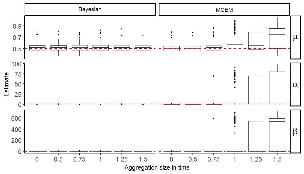
(a) Include problematic estimates in MC-EM

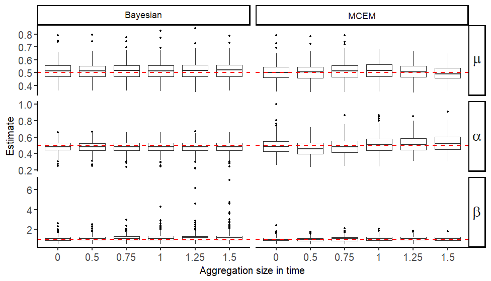
(b) Remove problematic estimates in MC-EM

Figure A.1: Boxplot for estimates of $\mu$,$\alpha$ and $\beta$ using our Bayesian approach (left) and the MC-EM approach. The horizonal red lines indicate the true values which corresponding to parameter set 2: $(\mu,\alpha,\beta)=(0.5,0.5,1)$

Table A.3: Results of the temporal simulation under additional parameter sets shown in (a), (b) and (c). The table shows the average posterior mean (“Estimate”), average 95% credible interval length (“CI length”), and coverage rate of the 95% credible interval (“Coverage”) for parameters $\mu,\alpha$ and $\beta$ of the Hawkes process, across 400 simulated data sets, for the exact data ($\Delta^{t}=0$), and temporal aggregations of different sizes.

	$\Delta^{t}$	Estimate	CI length	Coverage
$\mu$	0	0.1067	0.0781	0.9475
	0.5	0.1067	0.0781	0.9500
	0.75	0.1067	0.0782	0.9525
	1	0.1068	0.0784	0.9475
	1.25	0.1068	0.0783	0.9525
	1.5	0.1068	0.0786	0.9500
$\alpha$	0	0.8713	0.1827	0.9225
	0.5	0.8713	0.1827	0.925
	0.75	0.8711	0.1829	0.9225
	1	0.8712	0.183	0.9225
	1.25	0.8710	0.1829	0.9225
	1.5	0.8711	0.183	0.9275
$\beta$	0	1.0299	0.4936	0.9500
	0.5	1.0307	0.5011	0.9500
	0.75	1.0317	0.5074	0.9475
	1	1.0311	0.517	0.9550
	1.25	1.0382	0.5313	0.9375
	1.5	1.0383	0.5401	0.9600

(a) $(\mu,\alpha,\beta)=(0.1,0.9,1)$

	$\Delta^{t}$	Estimate	CI length	Coverage
$\mu$	0	0.7231	0.3115	0.9524
	0.75	0.7291	0.3159	0.9446
	0.5	0.7266	0.3145	0.9271
	1	0.7325	0.3173	0.9289
	1.25	0.7315	0.3211	0.9378
	1.5	0.7337	0.3182	0.9263
$\alpha$	0	0.2778	0.2895	0.9474
	0.75	0.2722	0.2929	0.932
	0.5	0.2746	0.2916	0.9196
	1	0.2691	0.2936	0.9289
	1.25	0.2700	0.2975	0.9301
	1.5	0.2667	0.2946	0.9158
$\beta$	0	1.4802	3.2491	0.9674
	0.75	2.0778	6.8470	0.9370
	0.5	1.7921	5.2139	0.9372
	1	2.534	9.8054	0.9442
	1.25	2.7988	11.1421	0.9223
	1.5	3.3263	13.8411	0.9342

(b) $(\mu,\alpha,\beta)=(0.7,0.3,1)$

	$\Delta^{t}$	Estimate	CI length	Coverage
$\mu$	0	0.905	0.3211	0.9700
	0.75	0.9072	0.3071	0.9750
	0.5	0.9087	0.3108	0.9650
	1	0.9079	0.3032	0.9800
	1.25	0.9073	0.2985	0.9725
	1.5	0.9051	0.2999	0.9750
$\alpha$	0	0.0985	0.2641	0.9600
	0.75	0.0958	0.2505	0.9825
	0.5	0.0943	0.2523	0.9775
	1	0.0950	0.2456	0.9875
	1.25	0.0962	0.2429	0.9875
	1.5	0.0979	0.2442	0.9775
$\beta$	0	4.6946	19.3281	0.9575
	0.75	6.5724	27.3506	0.9500
	0.5	6.1420	25.7129	0.9450
	1	7.2787	29.9935	0.9375
	1.25	7.6666	30.9145	0.9325
	1.5	7.9629	31.3147	0.9375

(c) $(\mu,\alpha,\beta)=(0.9,0.1,1)$

We run additional simulations for more challenging cases where data are generated from a very small or large branching ratio $\alpha$. In these cases, $\mu$ is chosen to be $1-\alpha$, so the expected total number of events are around 500 for all the cases we considered. The results are summarized in Table A.3. Estimation of $\mu$ and $\alpha$ is closed to unbiased in all cases, with adequate inferential performance and coverage near 95% throughout. We notice that the estimation for $\beta$ that drives the excitation density function deteriorates when $\alpha$ is small. However, that is true even when the exact data are known ($\Delta^{t}=0$) which illustrates that this is not an issue of the proposed approach, rather than the estimability of $\beta$ with a small number of offsprings. That said, for all aggregation sizes, the confidence intervals remain wide to manifest limited information on $\beta$, and coverage of the 95% credible intervals is close to 95%.

Simulation results for spatio-temporal data

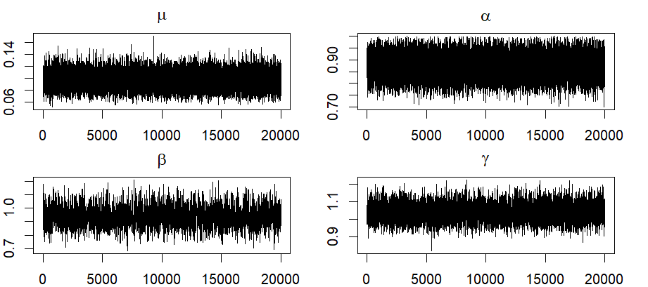
Figure A.2: Trace plots for a randomly chosen MCMC chain of the aggregated spatio-temporal model, when the data are generated from parameter set $(\mu,\alpha,\beta,\gamma)=(0.9,0.1,1,1)$ with aggregation sizes $\Delta^{t}=1.5$, $\Delta^{s}=1.5$

.

We considered spatio-temporal simulations with various choices of $\mu$, and $\alpha$. Specifically, for $\alpha=1-\mu$, we considered $\mu=0.1,0.3,0.5,0.7,0.9$, as we did in the temporal simulations. The parameters $\beta,\gamma$ were set to 1 throughout.

First, we should mention that we investigated MCMC convergence using the Rhat statistic and by investigating traceplots for the model parameters of randomly chosen simulated data sets. In Figure A.2 we show traceplots for the model parameters of a randomly chosen simulated data set from the spatio-temporal Hawkes process with parameters $(\mu,\alpha,\beta,\gamma)=(0.9,0.1,1,1)$, and the coarsest aggregation size $\Delta^{t}=\Delta^{s}=1.5$. We see that even in this challenging setting, the traceplots do not indicate any sign of lack of convergence.

Table A.4: The result of the spatio-temporal simulation. The table shows the average posterior mean (“Estimate”), average 95% credible interval length (“CI length”), and coverage rate of the 95% credible interval (“Coverage”) for parameters $\mu,\alpha$ and $\beta$, $\gamma$ of the Hawkes process, across 400 simulated data sets. Parameter set: $(\mu,\alpha,\beta,\gamma)=(0.1,0.9,1,1)$

$\mu$					$\alpha$
$\Delta^{t}$	$\Delta^{s}$	Estimate	CI length	Coverage	$\Delta^{t}$	$\Delta^{s}$	Estimate	CI length	Coverage
0	0	0.1026	0.0562	0.9375	0	0	0.877	0.1729	0.94
	0.5	0.1026	0.0561	0.9375		0.5	0.877	0.173	0.94
	1	0.1026	0.0561	0.93		1	0.8771	0.1729	0.94
	1.5	0.1026	0.0562	0.935		1.5	0.877	0.1729	0.94
0.5	0	0.1027	0.0562	0.935	0.5	0	0.877	0.1729	0.94
	0.5	0.1027	0.0562	0.935		0.5	0.877	0.1729	0.94
	1	0.1026	0.0562	0.9325		1	0.8771	0.1729	0.94
	1.5	0.1026	0.0562	0.9375		1.5	0.877	0.1729	0.94
1	0	0.1027	0.0562	0.93	1	0	0.877	0.173	0.94
	0.5	0.1027	0.0562	0.9325		0.5	0.877	0.173	0.94
	1	0.1026	0.0562	0.9325		1	0.8771	0.173	0.94
	1.5	0.1026	0.0562	0.935		1.5	0.8771	0.1729	0.94
1.5	0	0.1027	0.0562	0.9325	1.5	0	0.877	0.173	0.94
	0.5	0.1028	0.0562	0.9323		0.5	0.8768	0.1733	0.9425
	1	0.1028	0.0562	0.9323		1	0.8768	0.1733	0.9425
	1.5	0.1027	0.0563	0.9348		1.5	0.8768	0.1732	0.9425
$\beta$					$\gamma$
$\Delta^{t}$	$\Delta^{s}$	Estimate	CI length	Coverage	$\Delta^{t}$	$\Delta^{s}$	Estimate	CI length	Coverage
0	0	1.0199	0.2843	0.9375	0	0	1.0006	0.1392	0.9375
	0.5	1.0196	0.2853	0.9325		0.5	0.9997	0.1432	0.94
	1	1.0196	0.2882	0.9425		1	0.9977	0.1534	0.955
	1.5	1.0208	0.2923	0.94		1.5	0.9944	0.1675	0.935
0.5	0	1.0204	0.2887	0.935	0.5	0	1.0001	0.1416	0.9275
	0.5	1.0205	0.2902	0.93		0.5	0.9991	0.1454	0.94
	1	1.0205	0.2923	0.9325		1	0.9971	0.1553	0.9525
	1.5	1.0212	0.2963	0.93		1.5	0.9943	0.1688	0.9425
1	0	1.0228	0.2979	0.93	1	0	0.9998	0.1435	0.935
	0.5	1.0226	0.2986	0.9325		0.5	0.9991	0.1472	0.94
	1	1.0229	0.3009	0.9175		1	0.9973	0.1569	0.95
	1.5	1.0231	0.3043	0.92		1.5	0.9942	0.1699	0.94
1.5	0	1.0269	0.3092	0.945	1.5	0	0.9998	0.1453	0.9375
	0.5	1.0265	0.3099	0.9449		0.5	0.9988	0.149	0.9474
	1	1.0269	0.3124	0.9549		1	0.9969	0.1585	0.9474
	1.5	1.0269	0.3153	0.9373		1.5	0.9941	0.1716	0.9348

Table A.5: The result of the spatio-temporal simulation. The table shows the average posterior mean (“Estimate”), average 95% credible interval length (“CI length”), and coverage rate of the 95% credible interval (“Coverage”) for parameters $\mu,\alpha$ and $\beta$, $\gamma$ of the Hawkes process, across 400 simulated data sets. Parameter set: $(\mu,\alpha,\beta,\gamma)=(0.3,0.7,1,1)$

$\mu$					$\alpha$
$\Delta^{t}$	$\Delta^{s}$	Estimate	CI length	Coverage	$\Delta^{t}$	$\Delta^{s}$	Estimate	CI length	Coverage
0	0	0.3029	0.0969	0.95	0	0	0.6885	0.1491	0.9475
	0.5	0.3029	0.0969	0.95		0.5	0.6885	0.149	0.95
	1	0.3029	0.0969	0.9475		1	0.6885	0.1491	0.9525
	1.5	0.3031	0.097	0.9525		1.5	0.6884	0.1491	0.95
0.5	0	0.303	0.0969	0.9475	0.5	0	0.6885	0.1491	0.95
	0.5	0.3029	0.0969	0.95		0.5	0.6885	0.1491	0.95
	1	0.303	0.097	0.945		1	0.6884	0.1491	0.9525
	1.5	0.3031	0.0971	0.9475		1.5	0.6883	0.1492	0.9525
1	0	0.303	0.0969	0.95	1	0	0.6884	0.1491	0.95
	0.5	0.303	0.097	0.95		0.5	0.6884	0.1491	0.95
	1	0.303	0.097	0.9475		1	0.6884	0.1492	0.9525
	1.5	0.3032	0.0971	0.9475		1.5	0.6882	0.1492	0.955
1.5	0	0.3026	0.0969	0.9574	1.5	0	0.6888	0.1491	0.9521
	0.5	0.3026	0.0969	0.9529		0.5	0.6886	0.1491	0.9581
	1	0.3027	0.097	0.9555		1	0.6886	0.1492	0.9581
	1.5	0.3029	0.0971	0.9582		1.5	0.6884	0.1492	0.9608
$\beta$					$\gamma$
$\Delta^{t}$	$\Delta^{s}$	Estimate	CI length	Coverage	$\Delta^{t}$	$\Delta^{s}$	Estimate	CI length	Coverage
0	0	1.0204	0.2588	0.9475	0	0	0.9976	0.1296	0.9375
	0.5	1.0208	0.2597	0.95		0.5	0.9963	0.1336	0.9375
	1	1.0212	0.2613	0.9475		1	0.994	0.1447	0.9425
	1.5	1.0221	0.264	0.9375		1.5	0.9918	0.1605	0.94
0.5	0	1.0212	0.2629	0.955	0.5	0	0.9975	0.1314	0.93
	0.5	1.0217	0.2635	0.955		0.5	0.9962	0.1351	0.945
	1	1.0221	0.2648	0.955		1	0.994	0.1461	0.9325
	1.5	1.0229	0.2673	0.9425		1.5	0.992	0.1615	0.9375
1	0	1.0246	0.2723	0.94	1	0	0.9976	0.133	0.9375
	0.5	1.025	0.2728	0.94		0.5	0.9964	0.1367	0.94
	1	1.0252	0.2745	0.9425		1	0.9943	0.1473	0.925
	1.5	1.0266	0.2767	0.9325		1.5	0.9923	0.1625	0.935
1.5	0	1.0285	0.2842	0.9574	1.5	0	0.9973	0.1342	0.9309
	0.5	1.0276	0.2843	0.9634		0.5	0.9962	0.1379	0.9372
	1	1.0279	0.2856	0.9581		1	0.994	0.1483	0.9346
	1.5	1.0295	0.2884	0.9504		1.5	0.9921	0.1636	0.9295

Table A.6: Simulation results for spatio-temporal data. The table shows the average posterior mean (“Estimate”), average 95% credible interval length (“CI length”), and coverage rate of the 95% credible interval (“Coverage”) for parameters $\mu,\alpha$ and $\beta$, $\gamma$ of the Hawkes process, across 400 simulated data sets. Parameter set: $(\mu,\alpha,\beta,\gamma)=(0.5,0.5,1,1)$

$\mu$					$\alpha$
$\Delta^{t}$	$\Delta^{s}$	Estimate	CI length	Coverage	$\Delta^{t}$	$\Delta^{s}$	Estimate	CI length	Coverage
0	0	0.5029	0.125	0.95	0	0	0.4943	0.125	0.9425
	0.5	0.503	0.125	0.9475		0.5	0.4942	0.1251	0.9425
	1	0.503	0.1251	0.9475		1	0.4942	0.1251	0.945
	1.5	0.5032	0.1252	0.95		1.5	0.494	0.1252	0.9425
0.5	0	0.5029	0.125	0.95	0.5	0	0.4943	0.1251	0.9425
	0.5	0.5029	0.125	0.945		0.5	0.4943	0.1251	0.94
	1	0.503	0.1251	0.945		1	0.4942	0.1252	0.945
	1.5	0.5032	0.1252	0.95		1.5	0.494	0.1252	0.9425
1	0	0.5029	0.125	0.9475	1	0	0.4943	0.1252	0.9425
	0.5	0.503	0.1251	0.945		0.5	0.4942	0.1251	0.94
	1	0.503	0.1251	0.945		1	0.4941	0.1252	0.945
	1.5	0.5033	0.1252	0.9475		1.5	0.4939	0.1253	0.9425
1.5	0	0.503	0.1251	0.9475	1.5	0	0.4942	0.1252	0.945
	0.5	0.5031	0.1251	0.9525		0.5	0.4941	0.1251	0.9425
	1	0.5031	0.1252	0.9525		1	0.4941	0.1252	0.9425
	1.5	0.5033	0.1253	0.95		1.5	0.4939	0.1253	0.94
$\beta$					$\gamma$
$\Delta^{t}$	$\Delta^{s}$	Estimate	CI length	Coverage	$\Delta^{t}$	$\Delta^{s}$	Estimate	CI length	Coverage
0	0	1.0226	0.2888	0.955	0	0	0.9947	0.145	0.945
	0.5	1.0229	0.2892	0.9525		0.5	0.9936	0.15	0.9575
	1	1.0235	0.2911	0.95		1	0.9919	0.1645	0.9425
	1.5	1.0235	0.2932	0.9575		1.5	0.9867	0.1851	0.9475
0.5	0	1.0229	0.2935	0.955	0.5	0	0.9946	0.1463	0.95
	0.5	1.0231	0.2943	0.9575		0.5	0.9934	0.1513	0.9625
	1	1.0237	0.2959	0.955		1	0.9915	0.1654	0.9425
	1.5	1.0239	0.2982	0.965		1.5	0.9865	0.186	0.95
1	0	1.0242	0.3052	0.945	1	0	0.9945	0.1478	0.9425
	0.5	1.0244	0.3058	0.9525		0.5	0.9933	0.1527	0.9625
	1	1.0251	0.3076	0.9475		1	0.9916	0.1667	0.9475
	1.5	1.0255	0.3099	0.945		1.5	0.9862	0.1872	0.9525
1.5	0	1.0301	0.3231	0.9525	1.5	0	0.9948	0.149	0.95
	0.5	1.0305	0.3241	0.96		0.5	0.9936	0.1538	0.96
	1	1.0314	0.3258	0.9475		1	0.9916	0.1677	0.955
	1.5	1.0317	0.3284	0.96		1.5	0.9865	0.1882	0.95

Table A.7: Simulation results for spatio-temporal data. The table shows the average posterior mean (“Estimate”), average 95% credible interval length (“CI length”), and coverage rate of the 95% credible interval (“Coverage”) for parameters $\mu,\alpha$ and $\beta$, $\gamma$ of the Hawkes process, across 400 simulated data sets. Parameter set: $(\mu,\alpha,\beta,\gamma)=(0.7,0.3,1,1)$

$\mu$					$\alpha$
$\Delta^{t}$	$\Delta^{s}$	Estimate	CI length	Coverage	$\Delta^{t}$	$\Delta^{s}$	Estimate	CI length	Coverage
0	0	0.7037	0.148	0.9475	0	0	0.2976	0.0974	0.9375
	0.5	0.7038	0.148	0.9475		0.5	0.2975	0.0975	0.94
	1	0.7037	0.1482	0.9525		1	0.2975	0.0977	0.9325
	1.5	0.7039	0.1483	0.95		1.5	0.2973	0.0978	0.9375
0.5	0	0.7037	0.148	0.9475	0.5	0	0.2975	0.0974	0.9425
	0.5	0.7038	0.1481	0.9475		0.5	0.2974	0.0975	0.935
	1	0.7037	0.1481	0.9525		1	0.2974	0.0977	0.935
	1.5	0.7039	0.1483	0.9475		1.5	0.2973	0.0979	0.94
1	0	0.7037	0.1481	0.9475	1	0	0.2975	0.0975	0.9375
	0.5	0.7038	0.1481	0.95		0.5	0.2974	0.0975	0.935
	1	0.7038	0.1481	0.9525		1	0.2974	0.0977	0.9375
	1.5	0.704	0.1483	0.9475		1.5	0.2972	0.0979	0.935
1.5	0	0.7039	0.148	0.9475	1.5	0	0.2973	0.0975	0.945
	0.5	0.704	0.1481	0.9475		0.5	0.2972	0.0976	0.94
	1	0.7039	0.1482	0.9475		1	0.2973	0.0977	0.94
	1.5	0.7041	0.1484	0.945		1.5	0.2971	0.0979	0.94
$\beta$					$\gamma$
$\Delta^{t}$	$\Delta^{s}$	Estimate	CI length	Coverage	$\Delta^{t}$	$\Delta^{s}$	Estimate	CI length	Coverage
0	0	1.0289	0.3722	0.935	0	0	0.9957	0.1873	0.9475
	0.5	1.0293	0.3732	0.93		0.5	0.9953	0.1949	0.945
	1	1.0303	0.3766	0.9375		1	0.9951	0.2167	0.945
	1.5	1.0297	0.3791	0.95		1.5	0.989	0.2496	0.94
0.5	0	1.0302	0.3803	0.9375	0.5	0	0.9955	0.1885	0.9575
	0.5	1.0307	0.3819	0.9325		0.5	0.995	0.1961	0.945
	1	1.0314	0.3845	0.9325		1	0.9952	0.2178	0.945
	1.5	1.0309	0.3879	0.95		1.5	0.9886	0.2507	0.95
1	0	1.0371	0.403	0.94	1	0	0.9953	0.1898	0.9575
	0.5	1.0377	0.4048	0.94		0.5	0.9946	0.1971	0.9475
	1	1.0386	0.4072	0.945		1	0.9948	0.219	0.9475
	1.5	1.0385	0.41	0.94		1.5	0.9886	0.2518	0.9625
1.5	0	1.0463	0.4366	0.945	1.5	0	0.9944	0.1908	0.9525
	0.5	1.0466	0.4377	0.94		0.5	0.994	0.1984	0.95
	1	1.0476	0.4413	0.9425		1	0.9946	0.2202	0.9475
	1.5	1.0477	0.4449	0.9425		1.5	0.9881	0.2526	0.955

Table A.8: Simulation results for spatio-temporal data. The table shows the average posterior mean (“Estimate”), average 95% credible interval length (“CI length”), and coverage rate of the 95% credible interval (“Coverage”) for parameters $\mu,\alpha$ and $\beta$, $\gamma$ of the Hawkes process, across 400 simulated data sets. Parameter set: $(\mu,\alpha,\beta,\gamma)=(0.9,0.1,1,1)$

$\mu$					$\alpha$
$\Delta^{t}$	$\Delta^{s}$	Estimate	CI length	Coverage	$\Delta^{t}$	$\Delta^{s}$	Estimate	CI length	Coverage
0	0	0.9036	0.1676	0.9375	0	0	0.099	0.0583	0.95
	0.5	0.9036	0.1676	0.94		0.5	0.099	0.0584	0.955
	1	0.9037	0.1679	0.9375		1	0.0988	0.0587	0.95
	1.5	0.9039	0.168	0.9375		1.5	0.0986	0.0592	0.95
0.5	0	0.9036	0.1676	0.9375	0.5	0	0.0989	0.0584	0.95
	0.5	0.9036	0.1677	0.9375		0.5	0.0989	0.0585	0.95
	1	0.9038	0.1679	0.9375		1	0.0988	0.0588	0.9475
	1.5	0.904	0.168	0.9375		1.5	0.0986	0.0592	0.9475
1	0	0.9037	0.1677	0.9375	1	0	0.0988	0.0585	0.9475
	0.5	0.9038	0.1678	0.94		0.5	0.0988	0.0586	0.95
	1	0.9039	0.1679	0.9375		1	0.0986	0.0589	0.9525
	1.5	0.9042	0.1681	0.935		1.5	0.0984	0.0593	0.955
1.5	0	0.9039	0.1678	0.94	1.5	0	0.0986	0.0586	0.95
	0.5	0.9039	0.1678	0.94		0.5	0.0986	0.0587	0.9475
	1	0.9041	0.1679	0.94		1	0.0985	0.059	0.9475
	1.5	0.9044	0.1682	0.9375		1.5	0.0982	0.0594	0.9525
$\beta$					$\gamma$
$\Delta^{t}$	$\Delta^{s}$	Estimate	CI length	Coverage	$\Delta^{t}$	$\Delta^{s}$	Estimate	CI length	Coverage
0	0	1.0894	0.7538	0.9275	0	0	0.9991	0.3617	0.9575
	0.5	1.0894	0.7577	0.925		0.5	0.9974	0.377	0.96
	1	1.0927	0.7705	0.9225		1	0.9958	0.4279	0.95
	1.5	1.0933	0.785	0.93		1.5	0.9775	0.5123	0.9275
0.5	0	1.1000	0.7884	0.925	0.5	0	0.9984	0.3628	0.9675
	0.5	1.0994	0.7902	0.9225		0.5	0.9967	0.3785	0.955
	1	1.1033	0.8063	0.925		1	0.9953	0.4294	0.9575
	1.5	1.1045	0.8203	0.915		1.5	0.976	0.5131	0.935
1	0	1.1194	0.8866	0.9275	1	0	0.9982	0.3648	0.96
	0.5	1.1204	0.8916	0.93		0.5	0.9962	0.3803	0.9525
	1	1.1278	0.9188	0.925		1	0.9944	0.4315	0.9525
	1.5	1.1297	0.9377	0.9275		1.5	0.9751	0.5158	0.94
1.5	0	1.1875	1.1316	0.91	1.5	0	0.9989	0.3686	0.9625
	0.5	1.1878	1.1343	0.91		0.5	0.9969	0.3839	0.9525
	1	1.1971	1.1753	0.91		1	0.9953	0.4359	0.9525
	1.5	1.2105	1.2280	0.90		1.5	0.9769	0.5201	0.935

Tables A.4, A.5, A.6, A.7 and A.8 show the spatio-temporal simulation results for $\mu=0.1,0.3,0.5,0.7$ and $0.9$, respectively. Tables A.5 and A.6 correspond to parameter sets 1 and 2 in the manuscript, respectively, and they compliment the results and text shown in Section 4.2 of the manuscript. We see that the estimator performs well for $\mu$, $\alpha$ and $\gamma$ across all scenarios. Across all scenarios and parameters, coverage of the 95% credible intervals is close to 95%. Focusing on the most challenging scenario (Table A.8), we see that there is some bias in estimating $\beta$ when the branching ratio is small ($\alpha=0.1$). In this challenging setting estimating $\beta$ becomes harder with increasing length of credible intervals as the coarseness of temporal aggregation increases. However, coverage remains above 90% throughout.

Estimation of all parameters is improved when spatial information is available, compared to the situation with temporal data only. The length of the credible intervals in the spatio-temporal simulations are substantially lower than those in the temporal simulations for the common parameters ($\mu,\alpha,\beta$); to see this, compare the credible interval lengths in the results here to those in Table A.3 and section 4.1.

Simulation results for multivariate spatio-temporal data

Table A.9: The result of selected parameters ($\mu_{1},\alpha_{21},\beta_{11},\gamma_{21}$) in the multivariate spatio-temporal simulation. True parameter: ($\mu_{1},\alpha_{21},\beta_{11},\gamma_{21}$) = (0.3,0.3,1,1)

$\mu_{1}$					$\alpha_{21}$
$\Delta_{1}$	$\Delta_{2}$	Estimate	CI length	Coverage	$\Delta_{1}$	$\Delta_{2}$	Estimate	CI length	Coverage
0	0	0.3044	0.0983	0.9425	0	0	0.2994	0.089	0.9475
	0.75	0.3046	0.0998	0.9475		0.75	0.2993	0.0912	0.9475
	1	0.3047	0.1003	0.9525		1	0.2992	0.0921	0.9600
0.75	0	0.3047	0.0999	0.9375	0.75	0	0.2994	0.0916	0.9400
	0.75	0.3048	0.1006	0.9500		0.75	0.2993	0.0929	0.9525
	1	0.3047	0.1010	0.9475		1	0.2994	0.0938	0.9650
1	0	0.3051	0.1004	0.9400	1	0	0.2991	0.0927	0.9525
	0.75	0.3050	0.1011	0.9450		0.75	0.2993	0.0939	0.9500
	1	0.3053	0.1014	0.9575		1	0.2989	0.0947	0.9600
$\beta_{11}$					$\gamma_{12}$
$\Delta_{1}$	$\Delta_{2}$	Estimate	CI length	Coverage	$\Delta_{1}$	$\Delta_{2}$	Estimate	CI length	Coverage
0	0	1.0106	0.1729	0.9575	0	0	0.9966	0.2160	0.9250
	0.75	1.0103	0.1738	0.9525		0.75	0.9993	0.2469	0.9350
	1	1.0103	0.1742	0.9475		1	0.9957	0.2615	0.9525
0.75	0	1.0125	0.1807	0.9525	0.75	0	0.9953	0.2395	0.9375
	0.75	1.0123	0.1811	0.9400		0.75	0.9975	0.2625	0.9250
	1	1.0125	0.1814	0.9500		1	0.9937	0.2775	0.9550
1	0	1.0139	0.1846	0.9550	1	0	0.9943	0.2513	0.9425
	0.75	1.0135	0.1850	0.9475		0.75	0.9947	0.2739	0.9375
	1	1.0135	0.1854	0.9525		1	0.9912	0.2874	0.9475

In Table A.9 we show simulation results for data from a multivariate spatio-temporal Hawkes process. These results compliment the results and text shown in Section 4.3 of the manuscript. Since the number of parameters is large, we show results corresponding to a subset of them. We include parameters that represent background intensity ($\mu_{1}$), self-excitation ($\beta_{11}$), and cross-excitation ($\alpha_{21},\gamma_{21}$). Results for other parameters are similar.

We see that the posterior mean of all estimated parameters is, on average, near the true values, irrespective of aggregation size. Confidence intervals are wider under coarser aggregations. We see that the credible interval length for the parameters of the first component of the process $(\mu_{1},\beta_{11})$ is not affected by the aggregation size for the second process $(\Delta^{2})$. However, the credible interval length for the cross-excitation parameters ($\alpha_{21},\gamma_{21}$) is affected by the aggregation size of both processes. Coverage of 95% credible intervals is near the nominal level throughout.

Simulation results for Hawkes processes with Lomax kernel

In this section, we run simulations for Hawkes process with Lomax kernel. In other words, we assume $g(t)$ in the conditional intensity function of temporal Hawkes process and $g_{1}(t)$ are probability density functions of two-parameter Lomax distribution, which is in the form: $\frac{(p-1)c^{p-1}}{(t+c)^{p}}$. The $g_{2}(s)$ function in the spatio-temporal is still assumed to be a bivariate normal density. For both temporal and spatio-temporal cases, we generate 400 data sets with chosen parameters and fit the model with exact and aggregated data with varying aggregation sizes. We choose $\mu=0.3,\alpha=0.7$ for the temporal cases, and $\mu=0.5,\beta=0.5,\gamma=1$ for the spatio-temporal case. The parameters in the Lomax kernel was set to $c=1$, $p=3$ for both temporal and spatio-temporal cases. The mean excitation time under this Lomax specification is 1 (as for the exponential kernel with parameter 1 used in the other simulations).

Although the model is theoretically identifiable, we find that the parameters of the Lomax excitation function $c$ and $p$ are not individually well identified, even in the case of no aggregation. Thus, instead of studying $c$ and $p$ individually, we study whether the excitation function is estimated appropriately by focusing on quantiles of the Lomax distribution. We show results for the median here, though other quantiles were also studied. Firstly, we analyze the convergence of the MCMC by investigating trace plots of randomly selected data sets. Figure A.4 show the trace plots for parameter $\mu$, $\alpha$ and quantiles of the Lomax function in the most challenging case ($\Delta^{t}=1.5$) for temporal simulation, and Figure A.4 show the trace plot for parameter $\mu$, $\alpha$, $\gamma$ and the median of the Lomax function in the most challenging case ($\Delta^{t}=\Delta^{s}=1.5$) for the spatio-temporal simulation, for a random data set. Both plots show relative good convergence of the posterior samples, without any signs of convergence issues.

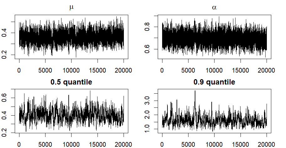
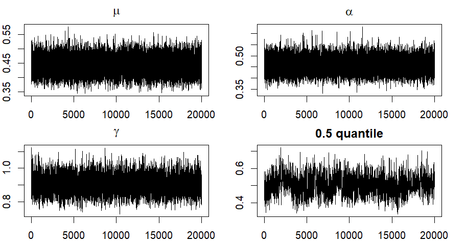
Figure A.3: Trace plots for a randomly chosen MCMC chain of the aggregated temporal model with Lomax kernel, when the data are generated from parameter set $(\mu,\alpha,c,p)=(0.3,0.7,1,3)$ with aggregation sizes $\Delta^{t}=1.5$

.

Figure A.4: Trace plots for a randomly chosen MCMC chain of the aggregated spatio-temporal model, when the data are generated from parameter set $(\mu,\alpha,c,p,\gamma)=(0.5,0.5,1,3,1)$ with aggregation sizes $\Delta^{t}=1.5$, $\Delta^{s}=1.5$

.

The simulation results for temporal and spatio-temporal simulations are shown in Table A.10 and Table A.11 respectively. We observed that the posterior mean for the $\alpha$, $\beta$, $\gamma$, and quantiles of the Lomax function are generally close to the true values in all scenarios, indicating that the estimates are overall unbiased and the fitted Lomax kernel function is close to the truth. The coverage rates for the model parameters $\mu,\alpha$ and $\gamma$ in the spato-temporal simulations are close to 0.95, while the coverage in the temporal simulations are a lower, ranging from 84–90%. An explanation for this is that it is difficult for the model to learn the branching structure when the kernel function is relatively flexible and the spatial information is unavailable. In the temporal simulations, the performance of the aggregated model is comparable to the model that uses the exact data. Similar to simulations for exponential kernel function, the credible interval lengths increases as the aggregation size increases. However, in the simulations for the exponential kernel function, the coverage rate for all parameters do not change much as the aggregation sizes increase, however, the coverage rate for the median of the Lomax function in the spatio-temporal simulations decreases from 0.925 to 0.8371 as the aggregation level changes from no aggregation to coarsest aggregation in time and space, indicating that the aggregation sizes have larger effects on the estimates for the Lomax kernel function than the exponential kernel function.

Table A.10: Results of the temporal simulation with Lomax kernel. The table shows the average posterior mean (“Estimate”), average 95% credible interval length (“CI length”), and coverage rate of the 95% credible interval (“Coverage”) for parameters $\mu,\alpha$ of the Hawkes process and 0.5 quantile of the Lomax distribution, across 400 simulated data sets, for the exact data ($\Delta^{t}=0$), temporal aggregations of different sizes. Parameter set: $(\mu,\alpha,c,p)=(0.3,0.7,1,3)$

	$\Delta^{t}$	Estimate	CI length	Coverage
$\mu$	0	0.3335	0.1743	0.8475
	0.5	0.3338	0.1749	0.84
	1	0.3352	0.1767	0.85
	1.5	0.3393	0.1813	0.8375
$\alpha$	0	0.6658	0.2074	0.9025
	0.5	0.6656	0.2083	0.9025
	1	0.6642	0.2101	0.89
	1.5	0.6599	0.2141	0.8925
0.5 quantile	0	0.389	0.2493	0.8875
	0.5	0.391	0.2642	0.885
	1	0.388	0.2874	0.8975
	1.5	0.3767	0.3164	0.8875

Table A.11: Simulation results for spatio-temporal data with Lomax kernel. The table shows the average posterior mean (“Estimate”), average 95% credible interval length (“CI length”), and coverage rate of the 95% credible interval (“Coverage”) for parameters $\mu,\alpha$ and $\gamma$ of the Hawkes process, and 0.5 quantile of the Lomax distribution, across 400 simulated data sets. Parameter set: $(\mu,\alpha,c,p,\gamma)=(0.5,0.5,1,3,1)$

$\mu$					$\alpha$
$\Delta^{t}$	$\Delta^{s}$	Estimate	CI length	Coverage	$\Delta^{t}$	$\Delta^{s}$	Estimate	CI length	Coverage
0	0	0.5071	0.1264	0.9475	0	0	0.4902	0.1255	0.925
	0.5	0.5072	0.1265	0.95		0.5	0.4901	0.1255	0.92
	1	0.5073	0.1266	0.95		1	0.49	0.1256	0.9175
	1.5	0.5075	0.1268	0.95		1.5	0.4899	0.1258	0.92
0.5	0	0.5075	0.1266	0.9525	0.5	0	0.4898	0.1256	0.9175
	0.5	0.5077	0.1266	0.9475		0.5	0.4897	0.1256	0.925
	1	0.5078	0.1267	0.9475		1	0.4896	0.1256	0.925
	1.5	0.508	0.1269	0.9525		1.5	0.4894	0.1258	0.9275
1	0	0.508	0.1267	0.9475	1	0	0.4894	0.1256	0.9175
	0.5	0.508	0.1267	0.945		0.5	0.4894	0.1256	0.9225
	1	0.5081	0.1269	0.95		1	0.4892	0.1257	0.92
	1.5	0.5083	0.127	0.95		1.5	0.489	0.1258	0.9175
1.5	0	0.5083	0.1268	0.9474	1.5	0	0.4889	0.1256	0.9248
	0.5	0.5083	0.1268	0.9474		0.5	0.4889	0.1256	0.9173
	1	0.5085	0.127	0.9499		1	0.4886	0.1257	0.9123
	1.5	0.5087	0.1271	0.9474		1.5	0.4885	0.1259	0.9198
$\gamma$					0.5 quantile
$\Delta^{t}$	$\Delta^{s}$	Estimate	CI length	Coverage	$\Delta^{t}$	$\Delta^{s}$	Estimate	CI length	Coverage
0	0	0.9955	0.1452	0.9425	0	0	0.4312	0.1606	0.925
	0.5	0.9957	0.1504	0.945		0.5	0.4313	0.1607	0.9225
	1	0.9928	0.1645	0.94		1	0.4313	0.1613	0.9225
	1.5	0.9893	0.185	0.9325		1.5	0.4315	0.1621	0.925
0.5	0	0.9965	0.1477	0.9475	0.5	0	0.439	0.1732	0.8975
	0.5	0.9956	0.1527	0.935		0.5	0.4392	0.1733	0.9025
	1	0.9923	0.1664	0.9325		1	0.4392	0.1737	0.895
	1.5	0.9882	0.1868	0.9325		1.5	0.4392	0.1742	0.8975
1	0	0.9951	0.1492	0.9425	1	0	0.4488	0.1928	0.87
	0.5	0.9947	0.1541	0.935		0.5	0.4486	0.1929	0.8725
	1	0.9917	0.1678	0.9425		1	0.449	0.1933	0.8725
	1.5	0.988	0.188	0.9425		1.5	0.4488	0.1936	0.8875
1.5	0	0.9949	0.1506	0.9248	1.5	0	0.4607	0.2121	0.8396
	0.5	0.9946	0.1554	0.9323		0.5	0.4606	0.2121	0.8546
	1	0.9918	0.169	0.9373		1	0.4612	0.2128	0.8421
	1.5	0.9878	0.1894	0.9398		1.5	0.4612	0.2128	0.8371

Computation efficiency

In this section, we show the computing time of the proposed method under the model specifications in Section E.1 and Section E.2. Table A.12 shows the shows the minimum, median and maximum time (in seconds) for running a single MCMC chain of 40,000 iterations, across 400 simulated data sets, for $\mu=0.1,0.9$ , $\alpha=1-\mu$ and $\beta=\gamma=1$. We observe that it takes longer time to fit the model on data sets with more offsprings (larger $\alpha$) when the total number events is the same, but for both parameter sets, the computing time for getting 40,000 posterior samples when time and locations are both aggregated are about 1.5 times the computing time when time and locations are exact.

To analyze the computing time for the aggregated temporal model relative to the size of the point pattern, we generate 50 data sets using $(\mu,\alpha,\beta)=(0.3,0.7,1)$ and $t=100,200,300,400,500.$ Then we fit aggregated model with $\Delta^{t}=1$ and record the time for getting 1,000 posteriors samples. Similarly, we generate 50 data sets from the spatio-temporal model with $\mu=0.3,\alpha=0.7,\beta=1,\gamma=1$, and $t=100,200,300,400,500$, and run 1,000 iterations for the aggregated data with $\Delta^{t}=\Delta^{s}=1.$ The relationships between computing time and number of events in aggregated temporal and aggregated spatio-temporal model are shown in Table A.12. We observe a linear trend between the computing time and the size of the point pattern for both temporal and spatio-temporal models.

Table A.12: The table shows the minimum, median and maximum time (in seconds) for running a single MCMC chain of 40,000 iterations, across 400 simulated data sets, for different parameter sets with $\beta=\gamma=1$

$\mu=0.1,\alpha=0.9$					$\mu=0.9,\alpha=0.1$
$\Delta^{t}$	$\Delta^{s}$	Min	Median	Max	$\Delta^{t}$	$\Delta^{s}$	Min	Median	Max
0	0	220	885	4384	0	0	335	615	959
	0.5	328	1313	6547		0.5	487	939	1358
	1	325	1329	6610		1	489	950	1354
	1.5	325	1310	6184		1.5	491	948	1332
0.5	0	340	1351	6563	0.5	0	536	1061	1498
	0.5	441	1783	8223		0.5	694	1376	1840
	1	442	1777	6715		1	700	1378	1879
	1.5	440	1837	5699		1.5	704	1379	1849
1	0	333	1412	4360	1	0	539	1059	1458
	0.5	441	1848	5757		0.5	699	1366	1866
	1	438	1835	5833		1	702	1367	1876
	1.5	438	1825	5696		1.5	705	1365	1867
1.5	0	334	1415	4386	1.5	0	544	1058	1823
	0.5	421	1830	4970		0.5	703	1360	1913
	1	431	1811	5133		1	616	1336	1879
	1.5	289	1743	5069		1.5	463	1303	1818

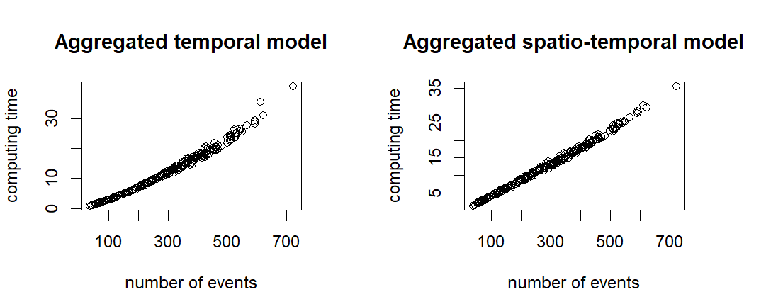
Figure A.5: Computing time (in seconds) of 1,000 posterior samples. The temporal data are generated using $(\mu,\alpha,\beta)=(0.3,0.7,1)$, with $t=100,200,300,400,500.$, The temporal data are generated using $(\mu,\alpha,\beta,\gamma)=(0.3,0.7,1,1)$, with $t=100,200,300,400,500.$ 50 data sets are generated, for each value of $t$.

Appendix F Trace plots in the analysis on insurgent attacks

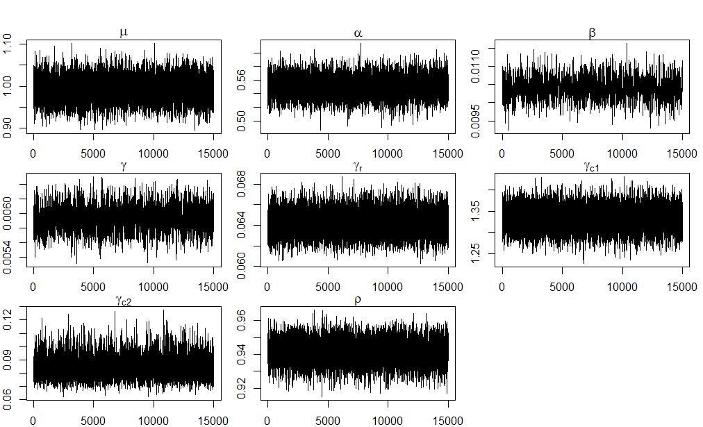
Figure A.6: Trace plots for parameters in the temporal model based on aggregated IED data with $\Delta^{t}=3/2$

Figure A.7: Trace plots for parameters in the spatio-temporal model based on aggregated IED data with $\Delta^{t}=24$, $\Delta^{s}=0.005$

In this section, we show the trace plots in Section 5 in the main manuscript. We run 20,000, 30,000 and 30,000 total iterations in temporal, spatio-temporal, and mutually exiciting spatio-temporal models respectively. Half of the samples are discared as burn-in samples, and there is no thinning. The trace plots of parameters in temporal and spatio-temporal model on IED attack with largest aggregation size are shown in Figure A.7 and Figure A.7 respectively. The trace plots for SAF attacks have similar patterns. The trace plots for parameters in the mutually exciting model on data with coarsest aggregation is presented in Figure A.8. We can see that these trace plots indicate good mixing, and there is no observable trend in all the plots.

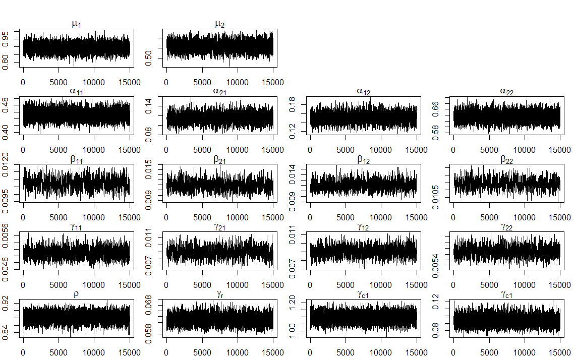
Figure A.8: Trace plots for parameters in the mutually exciting model based on aggregated IED and SAF data with $\Delta^{t}=24$, $\Delta^{s}=0.005$

Appendix G Forecasting the number of insurgent attacks

In this section, we show results that complement the text in Section 5.4. We assess the model performance by analyzing the ability of forecasting the number of events in the holdout period.

For the temporal analysis

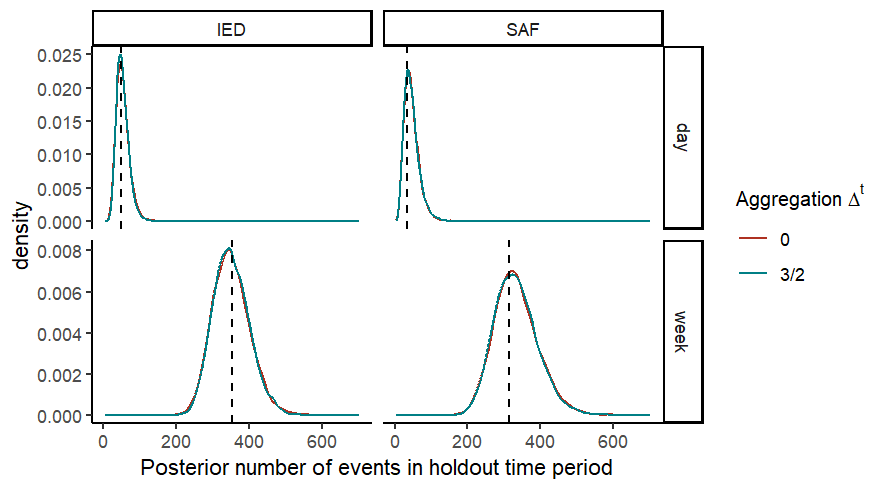
Figure A.9: Posterior predictive distribution of the number of IED and SAF attacks in one day (Dec 25,2006) and one week (Dec 25-31, 2006) based on the temporal models. The dashed dines indicate the true number of events.

For the temporal analysis, we evaluate the predictive posterior distribution in a relatively short time period (Dec 25, 2006), and the full holdout time period (Dec 25-31, 2006). Figure A.9 shows the predictive posterior distribution of number of IED and SAF attacks for the temporal model using the exact data, and data with the largest temporal aggregation ($\Delta^{t}$ = 1.5 hour). We see that the resulting distribution based on the exact data is very similar to that based on the coarsely aggregated data, and all the predictive posterior distributions are consistent with the true values, depicted by the vertical dashed lines.

For the spatio-temporal analysis, separately by type of attack

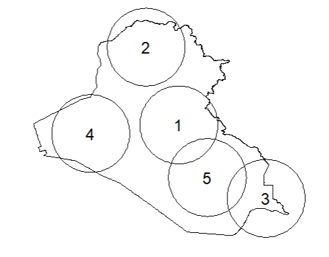
Figure A.10: The selected regions for the prediction

For the spatio-temporal analysis, we evaluate the predictive posterior distribution of number of IED and SAF attacks in five selected regions and in the full holdout time period. Those regions (Figure A.10) are chosen based on the locations of major cities of Iraq. In Figure A.11, we show the predictive posterior distributions of IED and SAF attacks in the selected regions using the exact data, and data with largest aggregation ($\Delta^{t}=$ 1 day, $\Delta^{s}$ = 0.005) from the separate spatio-temporal models. We observe that the predictive posterior distributions using exact data are very similar to those using aggregated data, and most posterior modes are close to the true value. The number of events in region 5 seems to be overestimated and the number of events in region 1 potentially underestimated by the model, but the estimates for the total number of events is relatively accurate.

The distribution of the spatial locations of attacks in the holdout time period can also be examined by applying the kernel density estimation on each sample from the predictive posterior distribution. The mean and standard deviations of the estimated intensity are shown in Figure A.12 for the model that uses the exact data and the model that uses the aggregated data. The points shown on the maps are the locations of the realized events in the holdout period. We see that the estimated intensities agree with the distribution of observed attacks in the holdout period, and the exact model and aggregated model yield very similar estimated intensities.

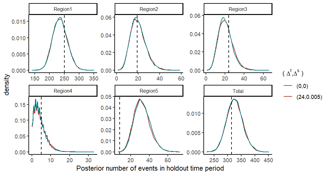
(a) SAF attacks

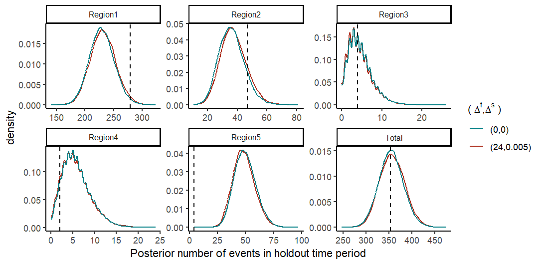
(b) IED attacks

Figure A.11: Posterior predictive distribution of the number of SAF in (a) and IED in (b) attacks in the last week in 2006 for different regions, based on exact data and aggregated data, using separate spatio-temporal models for SAF and IED attacks.

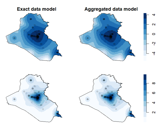
(a) SAF attacks

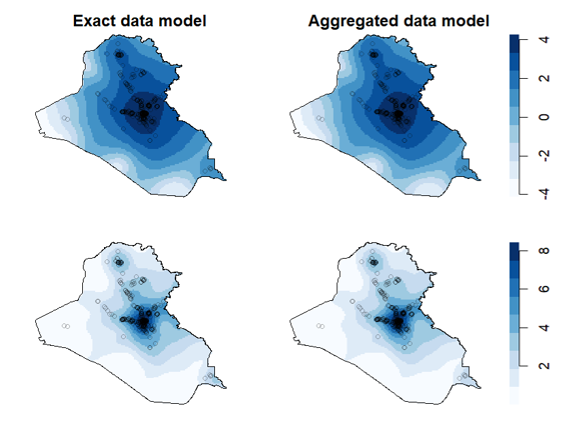
(b) IED attacks

Figure A.12: Logarithm of the mean of intensity predictions (top row) and standard deviation of intensity predictions (bottom row) for SAF (a) and IED (b) attacks in the last 7 days in 2006 based on the exact data (left column) and aggregated data with $\Delta^{t}=24$ and $\Delta^{s}=0.005$ (right column). The black points shows the true IED attack locations.

For the multivariate spatio-temporal analysis

We conduct the same analysis for the mutually exciting spatio-temporal model on IED and SAF attacks. The predictive posterior distribution number of SAF and IED attacks in the holdout period is shown in Figure A.13. The estimated intensities for SAF and IED attacks in the holdout period are shown in Figure A.14. The results from the multivariate model are similar to the results using separate spatio-temporal models for SAF and IED attacks.

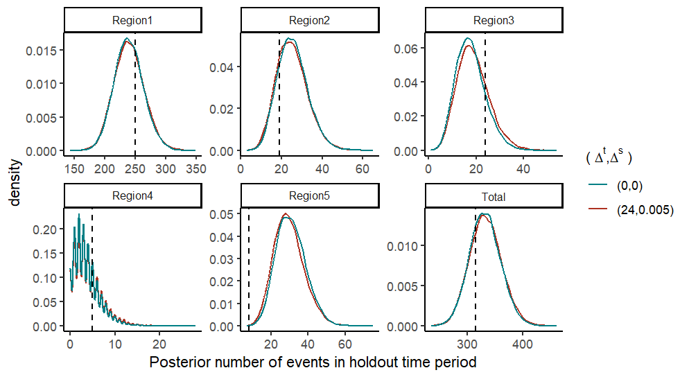
(a) SAF attacks

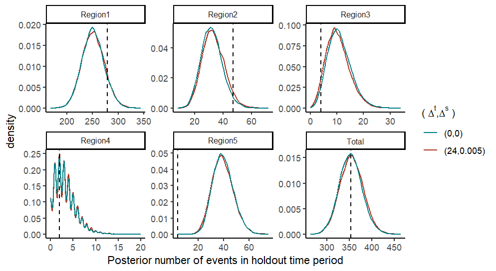
(b) IED attacks

Figure A.13: Posterior predictive distribution of the number of SAF (in (a)) and IED (in (b)) attacks in the last week in 2006 for different regions, by fitting the mutually exciting model, based on exact data and aggregated data.

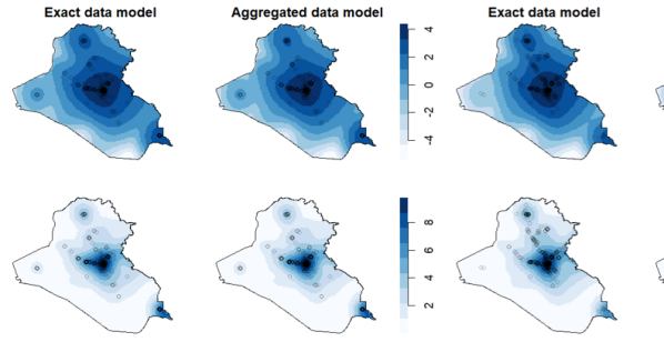
(a) SAF attacks

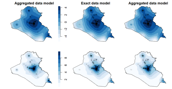
(b) IED attacks

Figure A.14: Logarithm of the mean of intensity predictions (top row) and standard deviation of intensity predictions (bottom row) for SAF attacks (left part) and IED attacks (right part) in the last week of 2006 based on the exact data(first and third columns) and aggregated data with $\Delta^{t}=24$ and $\Delta^{s}=0.005$ (second and fourth columns). The black points shows the true attack locations. The intensity is estimated based on the posterior predictive samples in the mutually exciting model.

References

- Aldor-Noiman et al. (2016) Aldor-Noiman, S., Brown, L. D., Fox, E. B., and Stine, R. A. (2016). Spatio-temporal low count processes with application to violent crime events. Statistica Sinica 1587–1610.
- Bu et al. (2022) Bu, F., Aiello, A. E., Xu, J., and Volfovsky, A. (2022). Likelihood-based inference for partially observed epidemics on dynamic networks. Journal of the American Statistical Association 117, 537, 510–526.
- Chiang et al. (2022) Chiang, W.-H., Liu, X., and Mohler, G. (2022). Hawkes process modeling of covid-19 with mobility leading indicators and spatial covariates. International journal of forecasting 38, 2, 505–520.
- Cronie and Särkkä (2011) Cronie, O. and Särkkä, A. (2011). Some edge correction methods for marked spatio-temporal point process models. Computational Statistics and Data Analysis 55, 7, 2209–2220.
- Darolles et al. (2019) Darolles, S., Le Fol, G., Lu, Y., and Sun, R. (2019). Bivariate integer-autoregressive process with an application to mutual fund flows. Journal of Multivariate Analysis 173, 181–203.
- Daryl and Vere-Jones (2003) Daryl, D. and Vere-Jones, D. (2003). An introduction to the theory of point processes: volume I: elementary theory and methods. Springer.
- Darzi et al. (2023) Darzi, A., Halldorsson, B., Hrafnkelsson, B., Ebrahimian, H., Jalayer, F., and Vogfjörð, K. S. (2023). Calibration of a bayesian spatio-temporal etas model to the june 2000 south iceland seismic sequence. Geophysical Journal International 232, 2, 1236–1258.
- Deutsch and Ross (2022) Deutsch, I. and Ross, G. J. (2022). Bayesian estimation of multivariate hawkes processes with inhibition and sparsity. arXiv preprint arXiv:2201.05009 .
- Diggle (2013) Diggle, P. J. (2013). Statistical analysis of spatial and spatio-temporal point patterns. CRC press.
- Fox et al. (2016) Fox, E. W., Schoenberg, F. P., and Gordon, J. S. (2016). Spatially inhomogeneous background rate estimators and uncertainty quantification for nonparametric hawkes point process models of earthquake occurrences. The Annals of Applied Statistics 10, 3, 1725–1756.
- Gelman and Rubin (1992) Gelman, A. and Rubin, D. B. (1992). Inference from iterative simulation using multiple sequences. Statistical science 7, 4, 457–472.
- Hawkes (1971) Hawkes, A. G. (1971). Spectra of some self-exciting and mutually exciting point processes. Biometrika 58, 1, 83–90.
- Hawkes and Oakes (1974) Hawkes, A. G. and Oakes, D. (1974). A cluster process representation of a self-exciting process. Journal of Applied Probability 11, 3, 493–503.
- Kirchner (2016) Kirchner, M. (2016). Hawkes and INAR () processes. Stochastic Processes and their Applications 126, 8, 2494–2525.
- Kirchner (2017) Kirchner, M. (2017). An estimation procedure for the hawkes process. Quantitative Finance 17, 4, 571–595.
- Kirchner and Bercher (2018) Kirchner, M. and Bercher, A. (2018). A nonparametric estimation procedure for the hawkes process: comparison with maximum likelihood estimation. Journal of Statistical Computation and Simulation 88, 6, 1106–1116.
- Lapham (2014) Lapham, B. M. (2014). Hawkes processes and some financial applications. Master’s thesis, University of Cape Town.
- Lewis and Mohler (2011) Lewis, E. and Mohler, G. (2011). A nonparametric em algorithm for multiscale hawkes processes. Journal of Nonparametric Statistics 1, 1, 1–20.
- Lewis et al. (2012) Lewis, E., Mohler, G., Brantingham, P. J., and Bertozzi, A. L. (2012). Self-exciting point process models of civilian deaths in iraq. Security Journal 25, 3, 244–264.
- Marsan and Lengline (2008) Marsan, D. and Lengline, O. (2008). Extending earthquakes’ reach through cascading. Science 319, 5866, 1076–1079.
- Ogata (1998) Ogata, Y. (1998). Space-time point-process models for earthquake occurrences. Annals of the Institute of Statistical Mathematics 50, 2, 379–402.
- Papadogeorgou et al. (2022) Papadogeorgou, G., Imai, K., Lyall, J., and Li, F. (2022). Causal inference with spatio-temporal data: estimating the effects of airstrikes on insurgent violence in iraq. Journal of the Royal Statistical Society Series B: Statistical Methodology 84, 5, 1969–1999.
- Porter and White (2012) Porter, M. D. and White, G. (2012). Self-exciting hurdle models for terrorist activity. The Annals of Applied Statistics 6, 1, 106–124.
- Rasmussen (2013) Rasmussen, J. G. (2013). Bayesian Inference for Hawkes Processes. Methodology and Computing in Applied Probability 15, 623–642.
- Reinhart (2018) Reinhart, A. (2018). A Review of Self-Exciting Spatio-Temporal Point Processes and Their Applications. Statistical Science 33, 3, 299—-318.
- Ross (2021) Ross, G. J. (2021). Bayesian estimation of the etas model for earthquake occurrences. Bulletin of the Seismological Society of America 111, 3, 1473–1480.
- Schoenberg (2013) Schoenberg, F. P. (2013). Facilitated estimation of etas. Bulletin of the Seismological Society of America 103, 1, 601–605.
- Shlomovich et al. (2021) Shlomovich, L., Cohen, E. A., and Adams, N. (2021). A parameter estimation method for multivariate aggregated hawkes processes. arXiv preprint arXiv:2108.12357 .
- Shlomovich et al. (2022) Shlomovich, L., Cohen, E. A., Adams, N., and Patel, L. (2022). Parameter estimation of binned hawkes processes. Journal of Computational and Graphical Statistics 1–11.
- Tucker et al. (2019) Tucker, J. D., Shand, L., and Lewis, J. R. (2019). Handling missing data in self-exciting point process models. Spatial statistics 29, 160–176.
- Veen and Schoenberg (2008) Veen, A. and Schoenberg, F. P. (2008). Estimation of space–time branching process models in seismology using an em–type algorithm. Journal of the American Statistical Association 103, 482, 614–624.
- Zhou et al. (2013) Zhou, K., Zha, H., and Song, L. (2013). Learning triggering kernels for multi-dimensional hawkes processes. In International conference on machine learning, 1301–1309. PMLR.