Solving High Dimensional Partial Differential Equations Using Tensor Type Discretization and Optimization Process

Abstract

In this paper, we propose a tensor type of discretization and optimization process for solving high dimensional partial differential equations. First, we design the tensor type of trial function for the high dimensional partial differential equations. Based on the tensor structure of the trial functions, we can do the direct numerical integration of the approximate solution without the help of Monte-Carlo method. Then combined with the Ritz or Galerkin method, solving the high dimensional partial differential equation can be transformed to solve a concerned optimization problem. Some numerical tests are provided to validate the proposed numerical methods. Keywords. Tensor type of trial function, direct numerical integration, optimization problem, high dimensional partial differential problem. AMS subject classifications. 65N30, 65N25, 65L15, 65B99.

1 Introduction

In this paper, we design a type of numerical method to solve high dimensional partial differential equations by using the standard finite element method and the optimization process. The key point is to use the tensor decomposition structure for representing the high dimensional trial function with some type of one dimensional basis functions. Solving partial differential equations is a basic and important task in many scientific and industrial applications. There also exist many high-dimensional PDEs such as many-body Schrödinger, Boltzmann equations, Fokker-Planck equations, stochastic PDEs (SPDEs), which are almost impossible solved by the traditional numerical methods.

Recently, the neural networks (NNs) based machine learning method is a popular way to solve the high-dimensional PDEs ([1, 5, 9, 10, 13]). The reason is that NNs can approximate any function if it is given enough parameters. The fully-connected neural network (FNN) is the most widely used architecture to build the functions for solving high-dimensional PDEs since its universal approximation property. So far, there are several types of FNN-based methods such as well-known deep Ritz [5], PINN [10] and DGM [13] for solving high-dimensional PDEs by designing different types of loss functions. Among these methods, the loss functions always include computing high-dimensional integrations for the functions defined by FNN. Direct numerical integration for the high-dimensional functions always meets the “curse of dimensionality” (CoD). Then Monte-Carlo method is always adopted to compute these high-dimensional integration with some types of sampling methods [5].

This paper proposes a new type of tensor type of discretization method to solve high dimensional partial differential equations without the help of Monte-Carlo process. The CANDECOMP/PARAFAC (CP) tensor decomposition [2, 7, 8] can build the low-rank approximation to high dimensional functions. The CP tensor decomposes can be considered as the higher-order extensions of the singular value decomposition (SVD) for the matrices. This means the SVD provides an idea to decompose the high-dimensional Hilbert space into the tensor product of several Hilbert spaces [12]. The tensor product decomposition has been used to establish low-rank approximations of operators and functions [3, 6, 11].

The aim of this paper is to propose a type of tensor type discretization (TTD) method to solve high-dimensional PDEs, which is based on the direct CP decomposition way to represent the trial functions for the high dimensional partial differential equations. With the help of some type of one dimensional basis functions, in the TTD, the trial function is constructed with the CP tensor decomposition way. Based on the tensor type of structure, we can design a efficient numerical integration for high dimensional trial functions. We will show, the computational work for the integration of these functions is only linear scale of the dimension. Based on this type of efficient numerical integrations, solving high dimensional partial differential equations can be transformed to the corresponding optimization problem. It is worth to mentioning that there is no tensor decomposition in TTD. We only use the tensor decomposition to build (or represent) the trial functions and then solve the deduced optimization problems with some type of iterative method. Finally, the TTD provides a way to overcome CoD in some sense for solving high-dimensional PDEs, which is the main motivation and contribution of this paper.

An outline of the paper goes as follows. In Section 2, we introduce the tensor type of method to build the high dimensional trial functions. Section 3 is devoted to proposing the TTD method for solving the high-dimensional boundary value problem with the efficient numerical integration for the trial functions. Some numerical examples are provided in Section 4 to show the validity and efficiency of the proposed numerical methods in this paper. Some concluding remarks are given in the last section.

2 Tensor type of trial function

In the section, we introduce the tensor type of way to build the trial function to approximate the solution of the high dimensional partial differential equations. The aim here is to build some type of low rank approximations for the high dimensional solutions.

In order to describe the way to build the high dimensional trail function to approximate the solution of partial differential equations, for $i=1,\cdots,d$, we use $\{\phi_{i,1}(x_{i}),\cdots,\phi_{i,N_{i}}(x_{i})\}$ to denote the basis of the finite dimensional space $\mathcal{V}_{i}$ which is a subspace of $H_{0}^{1}(\Omega_{i})$ on the one dimensional domain. Based on these basis, we can construct the discrete space $\mathcal{V}\subset H_{0}^{1}(\Omega)$ by using the tensor product way, i.e.,

$$\mathcal{V}:=\mathcal{V}_{1}\otimes\mathcal{V}_{2}\otimes\cdots\otimes\mathcal{V}_{d}\subset H_{0}^{1}(\Omega_{1}\times\cdots\times\Omega_{d})=H_{0}^{1}(\Omega).$$

With the help of tensor product way, we can also construct the basis as follows

$$\mathcal{V}={\rm span}\left\{\prod_{i=1}^{d}\phi_{i,j_{i}}(x_{i}),\ \ 1\leq j_{i}\leq N_{i}\right\}.$$ (1)

It is obvious that ${\rm dim}\mathcal{V}=\prod\limits_{i=1}^{d}N_{i}$ which depends exponentially on the dimension $d$. Then using these basis of the subspace $\mathcal{V}$ to do the discretization with the standard process of finite element method will leads to the linear algebraic equation with the degree of freedom $\prod\limits_{i=1}^{d}N_{i}$ which is an exponential function of the dimension $d$. This is the so called CoD.

In order to overcome the CoD, we use the tensor way to represent the trial function in this paper. The tensor way can reduce the complexity of the trail function representation. In the next section, the tensor way also brings the possibility to do the direct numerical integration for the high dimensional trial functions. Compared with the methods with Monte-Carlo integration, the tensor type discretization with the direct numerical integration can improve the stability and accuracy for solving high dimensional partial differential equations. In this paper, we use the tensor product way to represent the trial functions in the discrete space $\mathcal{V}$ as follows

$$v(x)=\sum_{j_{1}=1}^{N_{1}}\cdots\sum_{j_{d}=1}^{N_{d}}T_{j_{1},\cdots,j_{d}}\phi_{i,j_{1}}(x_{1})\cdots\phi_{i,j_{d}}(x_{d}),$$ (2)

where $T=(T_{j_{1},\cdots,j_{d}})_{1\leq j_{i}\leq N_{i}}\in\mathcal{R}^{N_{1}\times\cdots\times N_{d}}$ is a tensor with the order of $d$. There exists the following CP decomposition for the tensor $T$

$$T=\sum_{k=1}^{P}d_{k}v_{k,1}\otimes\cdots\otimes v_{k,d},$$ (3)

where $P$ denotes the rank of the function $v(x)$ and $v_{k,i}=(v_{k,i,j})_{1\leq j\leq N_{i}}$ is a vector of dimensional $N_{i}$, $1\leq i\leq d$.

Based on the CP decomposition (3) of the tensor $T$ and the basis for each space $\mathcal{V}_{i}$, we can use the following way to represent the function $v(x)\in\mathcal{V}$

$$v(x)=\sum_{k=1}^{P}\prod_{i=1}^{d}\left(\sum_{j=1}^{N_{i}}v_{k,i,j}\phi_{i,j}(x_{i})\right),$$ (4)

where the coefficient $v_{k,i,j}$ is the $k$-th components in the vector $v_{k,i}$ ($1\leq k\leq P$, $1\leq i\leq d$).

Based on this type of representation, we can build the discrete trial function for the high dimensional partial differential equation in the following way

$$u_{N}(x)=\sum_{k=1}^{P}\prod_{i=1}^{d}\left(\sum_{j=1}^{N_{i}}C_{k,i,j}\phi_{i,j}(x_{i})\right),$$ (5)

where $C_{k,i,j}$ denotes the unknown coefficients for the approximate solution. It is worth to mentioning that we do not generate the high dimensional mesh and high dimensional function explicitly. We only need to use the one dimensional basis function to build the high dimensional trial functions with the tensor product way.

This formula (5) provides a way to reduce the complexity for representing the trial function for the high dimensional partial differential equations. It is easy to know that the number of coefficients in (5) is

$$P\left(\sum\limits_{i=1}^{d}N_{i}\right).$$ (6)

Then, if the rank $P$ of the function $u_{N}(x)$ is polynomial scale of the dimension $d$, the number of coefficients $C_{k,i,j}$ does not depend exponentially on the dimension $d$. We will also find the decomposition (5) brings the possibility to do the direct numerical integration for these functions, which will be discussed in the next section.

The aim here is to give a framework to build the trial function for the high dimensional partial differential equations. With this framework, we can choose different type of basis functions $\phi_{i,j}(x_{i})$ to construct the trial function as in (5). For example, finite element basis, spectral basis, wavelet basis can all be chosen here. Furthermore, the neural network function is also an important candidate to build the trial function for the high dimensional partial differential equation. This will be discussed in our another paper.

3 Solving high-dimensional boundary value problem

In this section, we will show the first application of the tensor type discretization method. Here we are concerned with solving the high dimensional second order elliptic partial differential equation with homogeneous Neumann boundary condition: Find $u\in H^{1}(\Omega)$ such that

$$\left\{\begin{array}[]{rcl}-\Delta u+\pi^{2}u&=&2\pi^{2}\sum\limits_{k=1}^{d}\cos(\pi x_{k}),\ \ \ x\in\Omega,\\ \frac{\partial u}{\partial\mathbf{n}}&=&0,\ \quad\quad\quad\quad\quad\quad\ \ \ x\in\partial\Omega,\end{array}\right.$$ (9)

where the computing domain $\Omega=[0,1]^{d}$. Then the exact solution is

$$u(x)=\sum_{k=1}^{d}\cos(\pi x_{k}).$$

It is well known that the problem (9) is equivalent to the following minimization problem

$$u(x) = \arg\min_{v\in H^{1}(\Omega)}I(v)$$ (10)

$$:= \arg\min_{u\in H^{1}(\Omega)}\left[\frac{1}{2}\int_{\Omega}\left(|\nabla v|^{2}+\pi^{2}v^{2}\right)dx-\int_{\Omega}2\pi^{2}\sum_{k=1}^{d}\cos(\pi x_{k})vdx\right].$$

In order to solve the optimization problem (10), we build the tensor type of trial function $u_{N}(x)$ in (5), and define the set of all possible values of coefficients $C_{k,i,j}$.

The trial function set $V$ is modeled by the parameters $C_{k,i,j}$, which take all the possible values and it is easy to satisfy the condition $V\subset H_{0}^{1}(\Omega)$. The approximate solution $u_{N}(x)$ for (10) can be defined as the solution of the following optimization problem

$$u_{N}(x) := \arg\min_{u_{N}\in V}\left[\frac{1}{2}\int_{\Omega}\left(|\nabla v|^{2}+\pi^{2}v^{2}\right)dx-\int_{\Omega}2\pi^{2}\sum_{k=1}^{d}\cos(\pi x_{k})vdx\right].$$ (11)

Note that the terms of (11) includes the high dimensional integration. It is well known that the high dimensional integration has the CoD. Always, the Monte-Carlo method is used to do these high dimensional integration. Fortunately, since the tensor decomposition structure of the trail function in this paper, we can do the direct high dimensional integration without Monte-Carlo process.

From the definition of $u_{N}(x)$ in (5), we have the following representation for $u_{N}^{2}(x)$

$$u_{N}^{2}(x) = \sum_{k=1}^{P}\prod_{i=1}^{d}\left(\sum_{j=1}^{N_{i}}C_{k,i,j}\phi_{i,j}\left(x_{i}\right)\right)\sum_{\ell=1}^{P}\prod_{m=1}^{d}\left(\sum_{n=1}^{N_{m}}C_{\ell,m,n}\phi_{m,n}\left(x_{m}\right)\right)$$ (12)

$$= \sum_{k=1}^{P}\sum_{\ell=1}^{P}\prod_{i=1}^{d}\left(\sum_{j=1}^{N_{i}}C_{k,i,j}\phi_{i,j}\left(x_{i}\right)\right)\left(\sum_{n=1}^{N_{i}}C_{\ell,i,n}\phi_{i,n}\left(x_{i}\right)\right).$$

Then the following quadrature scheme holds

$$\int_{\Omega}u_{N}^{2}(x)dx = \sum_{k=1}^{P}\sum_{\ell=1}^{P}\prod_{i=1}^{d}\int_{\Omega_{i}}\left(\sum_{j=1}^{N_{i}}C_{k,i,j}\phi_{i,j}\left(x_{i}\right)\right)\left(\sum_{n=1}^{N_{i}}C_{\ell,i,n}\phi_{i,n}\left(x_{i}\right)\right)dx_{i}$$ (13)

$$= \sum_{k=1}^{P}\sum_{\ell=1}^{P}\prod_{i=1}^{d}\left(\sum_{j=1}^{N_{i}}\sum_{n=1}^{N_{i}}C_{k,i,j}C_{\ell,i,n}\int_{\Omega_{i}}\phi_{i,j}\left(x_{i}\right)\phi_{i,n}\left(x_{i}\right)dx_{i}\right).$$

From (13), in order to do the high dimensional integration $\int_{\Omega}u_{N}^{2}(x)dx$, we only need to compute the one dimensional integration $\int_{\Omega_{i}}\phi_{i,j}\left(x_{i}\right)\phi_{i,n}\left(x_{i}\right)dx_{i}$ for $1\leq j,n\leq N_{i}$ and $1\leq i\leq d$. Other terms in (11) can be treated with the similar way in (13).

Theorem 1.

Assume that the function $u(x)$ is defined as (5) in the $d$-dimensional tensor product domain $\Omega$. Let $N:=\max\{N_{1},\cdots,N_{d}\}$ and $T_{1}$ denote the computational complexity for the following $1$-dimensional integration

$$\int_{\Omega_{i}}\phi_{i,j}(x_{i})\phi_{i,n}(x_{i})dx_{i},\ \ \ 1\leq j,n\leq N_{i},\ i=1,\cdots,d.$$ (14)

The computational complexity for the numerical integration (13) can be bounded by $\mathcal{O}\big{(}dT_{1}P^{2}N\big{)}$, which is the polynomial scale of the dimension $d$.

Remark 1.

For some special equations, we can choose the basis with orthogonal property such that the computational complexity for the integration in Theorem 1 can be reduced to $\mathcal{O}\big{(}dT_{1}PN\big{)}$.

If $u_{N}(x)$ does not have the tensor form, when using the same quadrature scheme, it is easy to know that the computational complexity for the high dimensional integration depends exponentially on the dimension.

In this paper, the gradient descent (GD) method is adopted to solve the optimization problem (11). The GD scheme can be described as follows:

$$\theta^{(k+1)}=\theta^{(k)}-\eta\nabla\mathcal{R}(u^{(k)}(x)),$$ (15)

where $\theta^{(k)}$ denotes the parameters after the $k$-th GD step, $\eta$ is the learning rate (step size). Actually, in this paper, we use the alternating coordinate gradient descent method to solve the optimization problem (11) since in each dimensional, the target function is an quadratic form and it is can be easily optimized.

Fortunately, based on the tensor structure in this paper, Theorem 1 shows that the high dimensional numerical integration does not encounter CoD since the computational work can be bounded by the polynomial scale of dimension $d$. Due to the high accuracy of high dimensional integration and then the target function, the high accuracy of the tensor type discretization method can be guaranteed.

4 Numerical experiments

In this section, we come to investigate the numerical performance of the tensor type discretization method for the problem (9). The aim here is to check the efficiency and accuracy of the proposed numerical method in this paper.

For the simplicity, the linear finite element basis functions [4] are adopted to act as the basis $\phi_{i,j}(x_{i})$ for $1\leq j\leq N_{i}$ and $1\leq i\leq d$ for the tensor type of trial functions (5). Since the exact solution $u$ is known, we can check the exact error for the approximate solution with the help of the numerical integration for the tensor type functions. In order to show the convergence behavior and accuracy of approximations by tensor type discretization, we define the $H^{1}(\Omega)$ and $L^{2}(\Omega)$ error estimates as follows

$${\rm Err}_{H^{1}}:=\frac{\|u(x)-u_{N}(x)\|_{1}}{\|f\|_{0}},\ \ \ {\rm Err}_{L^{2}}:=\frac{\|u(x)-u_{N}\|_{0}}{\|f\|_{0}}.$$

In all tests, we set the rank $P=2d$. All the numerical tests are done by the laptop with I7 CPU (2.8G) and 8G memory and the code is written with Python. The optimization problem (11) is solved with the alternating coordinate gradient descent method.

In order to show the comparison with the standard finite element method, we fist show the numerical results for the three dimensional case $d=3$. The corresponding numerical results are shown in Figure 1.

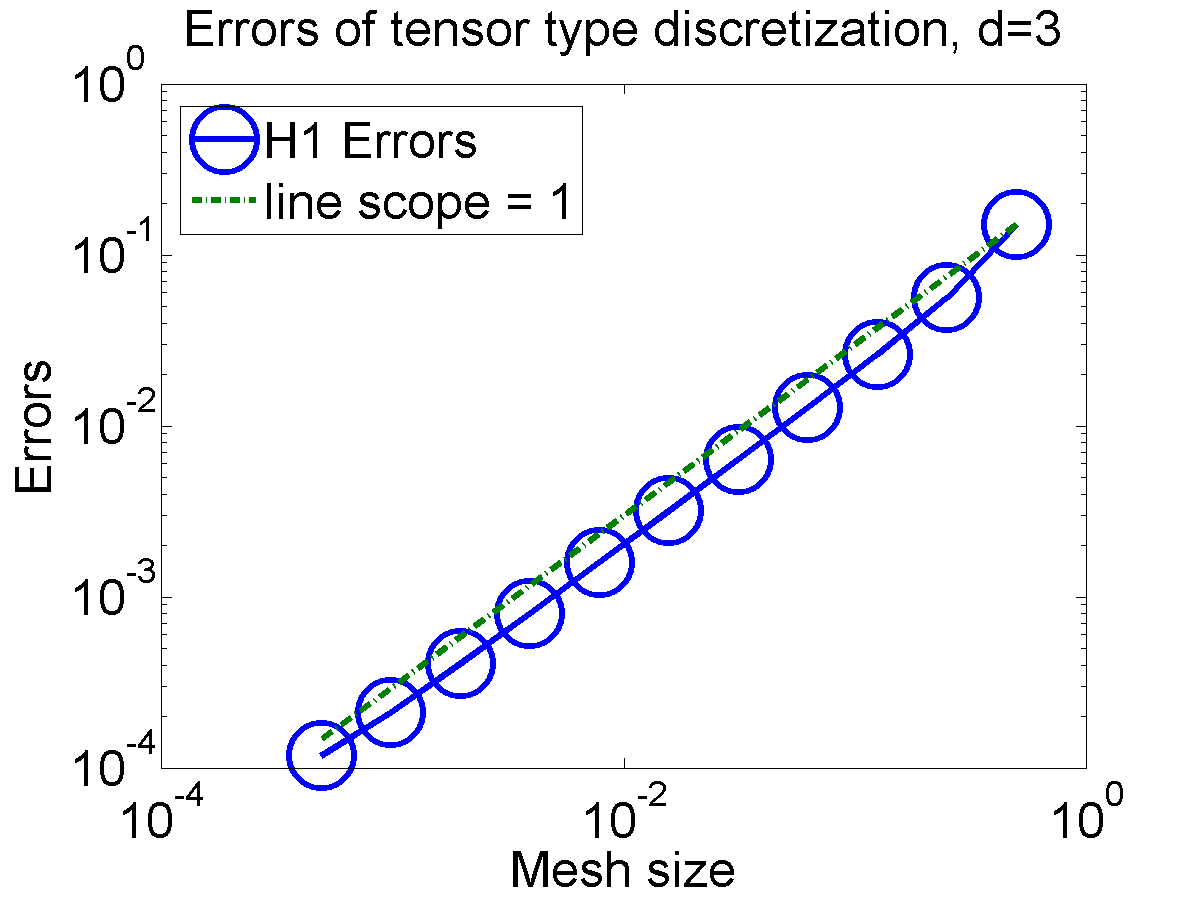
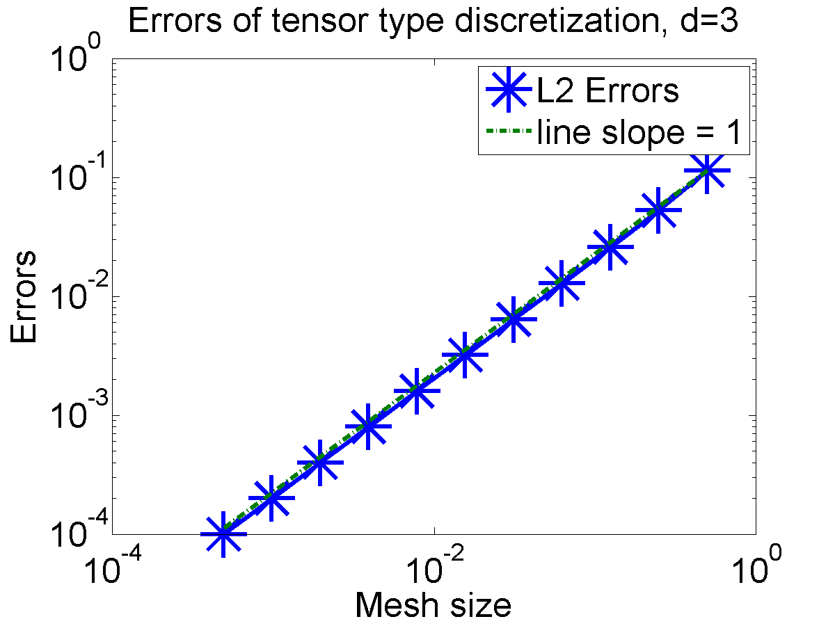
Figure 1: Errors for the three dimensional case with the tensor type of discretization method with the sequence of mesh sizes $h=[1/2,1/4,1/8,1/16,1/32,1/64,1/128,1/256,1/512,1/1024,1/2048]$.

From Figure 1, we can find that the tensor type of discretization can also get the optimal convergence order for the $H^{1}(\Omega)$ norm errors. Different form the standard finite element method, the $L^{2}(\Omega)$ errors can also only have the first convergence order. As we know, in this case, we can also use a finite element packages to solve the three dimensional boundary value problem (9). But in order to obtain the same accuracy, we need to generate the three dimensional mesh with the mesh size $h=1/2048$. Then the corresponding number of tetrahedral is $6\times 2048^{3}\approx 5.15\times 10^{10}$ and we must use the high performance computer and the parallel method. For the comparison, with the tensor type of discretization, we only need to use a laptop to solve the same problem.

In this section, we also do the numerical experiments for the five dimensional boundary value problem (9). The corresponding numerical results are shown in Figure 2.

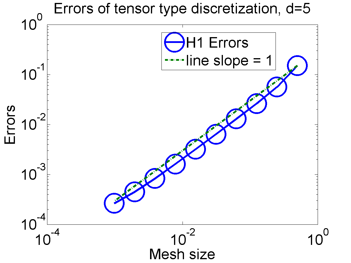
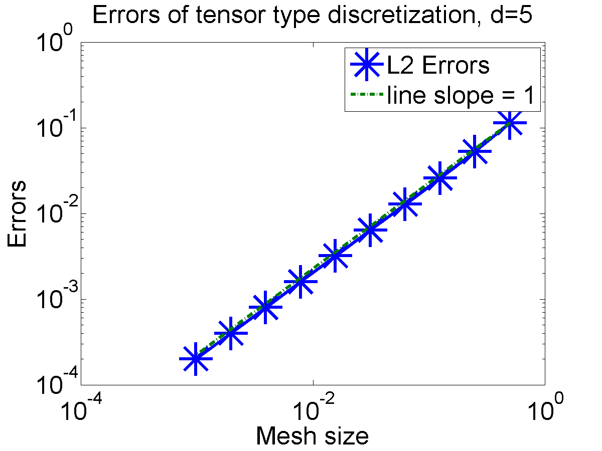
Figure 2: Errors for the five dimensional case with the tensor type of discretization method with the sequence of mesh sizes $h=[1/2,1/4,1/8,1/16,1/32,1/64,1/128,1/256,1/512,1/1024]$.

From Figure 2, we can also find that the tensor type discretization method can obtain the optimal convergence order for the $H^{1}(\Omega)$ error estimates and the $L^{2}(\Omega)$ errors also has only first order convergence.

5 Conclusions

In this paper, we present the tensor type of discretization method for solving high dimensional partial differentia equations. Since the proposed discretization method has the tensor product structure, we can do the direct numerical integration without the help of Monte-Carlo process for the high dimensional trial functions and their inner-products. The direct numerical integration for high dimensional trial functions can improve the stability and accuracy for solving high dimensional partial differential equations. We believe the ability of direct numerical integration will bring more applications.

Based on the constructing way and numerical integration method in this paper, we can do the following extensions:

1. Different types of basis functions can be adopted to build the trial functions for solving high dimensional partial differential equations.

2. TThe neural network can be used to construct the tensor type discretization here. This means the neural network can be combined with the tensor type discretization to build a new type of machine learning method for solving high dimensional partial differential equations.

3. Since the direct numerical integration for the trial functions, we can do the posteriori error estimate for the approximate solutions [4]. This also provide an adaptive way to chose the rank for building the trial functions.

4. Since we need to solve the nonlinear optimization problem for the tensor type discretization method, the augmented subspace method [14, 15] can be used to improve the efficiency of solving the nonlinear optimization problems.

More applications to other types of problems will also be considered in the future.

References

- [1] M. Baymani, S. Effati, H. Niazmand and A. Kerayechian, Artificial neural network method for solving the Navier-Stokes equations. Neural Comput & Applic., 26(4) (2015), 765–763.
- [2] G. Beylkin and M. J. Mohlenkamp, Numerical operator calculus in higher dimensions. Proceedings of the National Academy of Sciences, 99(16) (2002), 10246–10251.
- [3] G. Beylkin and M. J. Mohlenkamp, Algorithms for numerical analysis in high dimensions. SIAM J. Sci. Comput., 26(6) (2005), 2133–2159.
- [4] D. Braess, Finite Elements: Theory, Fast Solvers, and Applications in Solid Mechanics (3rd ed.). Cambridge: Cambridge University Press, 2007.
- [5] W. E and B. Yu, The deep Ritz method: a deep-learning based numerical algorithm for solving variational problems. Commun. Math. Stat., 6 (2018), 1–12.
- [6] W. Hackbusch and B. N. Khoromskij, Tensor-product approximation to operators and functions in high dimensions. J. Complexity, 23(4-6) (2007), 697–714.
- [7] D. Hong and T. G. Kolda and J. A. Duersch, Generalized canonical polyadic tensor decomposition. SIAM Review, 62(1) (2020), 133–163.
- [8] T. G. Kolda and B. W. Bader, Tensor decompositions and applications. SIAM Review, 51(3) (2009), 455–500.
- [9] I. E. Lagaris, A. C. Likas and G. D. Papageorgiou, Neural-network methods for boundary value problems with irregular boundaries. IEEE Trans. Neural Networks, 11 (2000), 1041–1049.
- [10] M. Raissi, P. Perdikaris and G. E. Karniadakis, Physics informed deep learning (part I): Data-driven solutions of nonlinear partial differential equations. arXiv:1711.10561, 2017.
- [11] M. J. Reynolds, A. Doostan and G. Beylkin, Randomized alternating least squares for canonical tensor decompositions: Application to a PDE with random data. SIAM J. Sci. Comput., 38(5) (2016), A2634–A2664.
- [12] R. A. Ryan, Introduction to tensor products of Banach spaces. London: Springer, 2002.
- [13] J. Sirignano and K. Spiliopoulos, DGM: A deep learning algorithm for solving partial differential equations. J. Comput. Phys., 375 (2018), 1339–1364.
- [14] H. Xie, A multigrid method for eigenvalue problem. Journal of Computational Physics, 274(1) (2014), 550–561.
- [15] H. Xie, An augmented subspace method and its applications. Journal on Numerical Methods and Computer Applications, 41(3) (2020), 169–191.