Self-consistent Quantum Iteratively Sparsified Hamiltonian method (SQuISH):
A new algorithm for efficient Hamiltonian simulation and compression

Abstract

It is crucial to reduce the resources required to run quantum algorithms and simulate physical systems on quantum computers due to coherence time limitations. With regards to Hamiltonian simulation, a significant effort has focused on building efficient algorithms using various factorizations and truncations, typically derived from the Hamiltonian alone. We introduce a new paradigm for improving Hamiltonian simulation and reducing the cost of ground state problems based on ideas recently developed for classical chemistry simulations. The key idea is that one can find efficient ways to reduce resources needed by quantum algorithms by making use of two key pieces of information: the Hamiltonian operator and an approximate ground state wavefunction. We refer to our algorithm as the Self-consistent Quantum Iteratively Sparsified Hamiltonian (SQuISH). By performing our scheme iteratively, one can drive SQuISH to create an accurate wavefunction using a truncated, resource-efficient Hamiltonian. Utilizing this truncated Hamiltonian provides an approach to reduce the gate complexity of ground state calculations on quantum hardware. As proof of principle, we implement SQuISH using configuration interaction for small molecules and coupled cluster for larger systems. Through our combination of approaches, we demonstrate how SQuISH performs on a range of systems, the largest of which would require more than 200 qubits to run on quantum hardware. Though our demonstrations are on a series of electronic structure problems, our approach is relatively generic and hence likely to benefit additional applications where the size of the problem Hamiltonian creates a computational bottleneck.

I Introduction

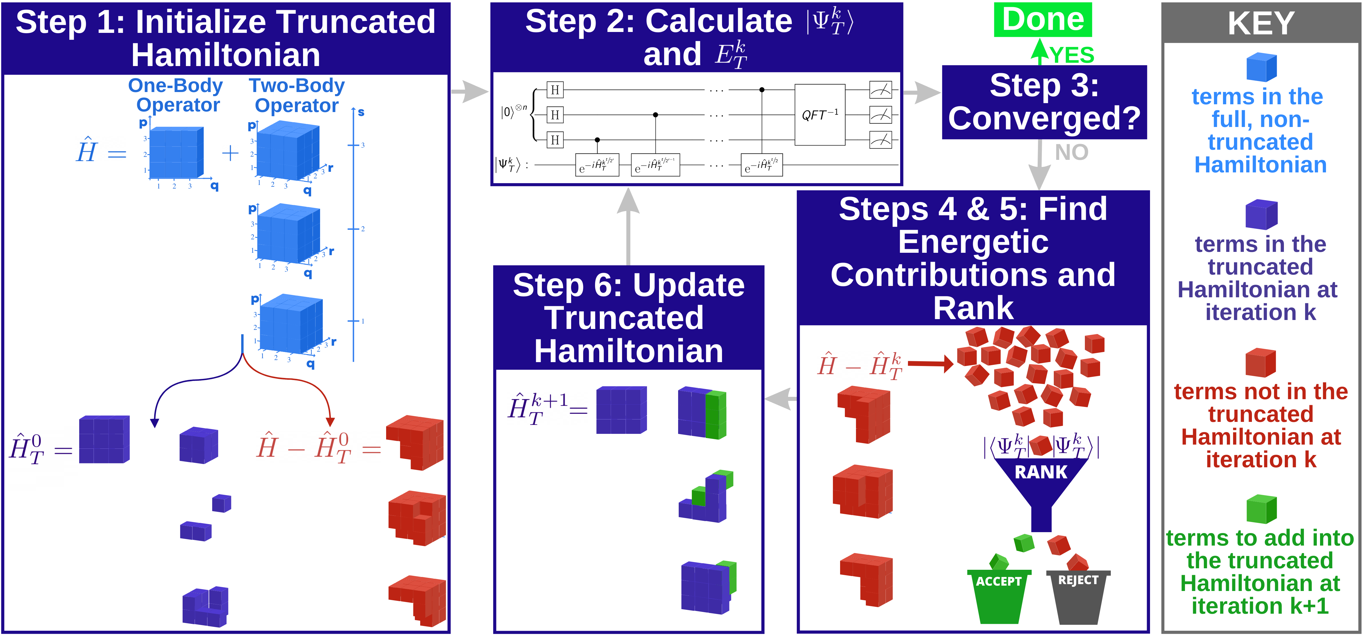
Figure 1: Schematic diagram of SQuISH (see Section III for detailed explanation of each step). The Hamiltonian is illustrated with a three dimensional representation of the 2D one-body operator and 4D two-body operator. Each cube represents a single Hamiltonian term, $h_{pq}\hat{a}_{p}^{\dagger}\hat{a}_{q}$ or $h_{pqrs}\hat{a}_{p}^{\dagger}\hat{a}_{q}^{\dagger}\hat{a}_{r}\hat{a}_{s}$. This figure gives a hypothetical example of SQuISH applied to a 3 spatial orbital molecule. The initial Hamiltonian (in Step 1) includes all one-body terms and a subset of the two-body terms as an example. QPE is shown as possible quantum algorithm used for the truncated Hamiltonian ground state calculation.

The electronic structure problem gives insight into reaction rates, geometry of stable structures, and determination of optical properties, among many others Helgaker et al. (2012); McArdle et al. (2020a); Bauer et al. (2020). Classical methods such as full configuration interaction, which simulate the entire Hilbert space, are limited to small systems due to the computational scaling with increasing orbitals and electrons.  Thøgersen and Olsen (2004); Alán et al. (2005). While there are classical approaches to calculate such solutions approximately Szabo and Ostlund (2012); Helgaker et al. (2014), it is anticipated that quantum computers may offer an exponential advantage in calculating exact solutions for some quantum computational chemistry problems Alán et al. (2005); McArdle et al. (2020b).

Quantum phase estimation (QPE) Kitaev (1995); Abrams and Lloyd (1999) is a promising quantum algorithm to solve electronic structure problems near-exactly. QPE and its variants evolve a quantum state in time under a given Hamilton, which amounts to solving the Schrödinger equation for different times. A few of the most prominent time evolution methods are Trotter-Suzuki product formulas Trotter (1959); Suzuki (1976); Lloyd (1996); Aharonov and Ta-Shma (2003); Berry et al. (2007); Hadfield and Papageorgiou (2018); Childs et al. (2021a), related randomized approaches such as qDRIFT Zhang (2012); Campbell (2019); Childs et al. (2019), and post-Trotter approaches such as qubitization Low and Chuang (2017, 2019).

If we consider Trotterization based methods, performing just one Trotter step for a molecule scales as $N^{4}$ (the number of Hamiltonian terms) if approximations on the Hamiltonian are not used. Here $N$ is the number of spin orbitals used for a given system, typically much larger than the number of electrons as more accurate basis sets are employed Seeley et al. (2012a); Hastings et al. (2015). Generally, the cost of simulating a Hamiltonian using these methods depends on the number of terms as well as their magnitudes with respect to particular operator norms Childs et al. (2021b); Loaiza et al. (2022).

For the most part, there is a direct correspondence between quantum circuit depth and requisite physical coherence time. Due to interaction with the environment, even if one has a quantum device with sufficiently many qubits, maintaining a quantum state long enough to perform calculations reliably is a significant challenge Zurek (1981); Joos and Zeh (1985); Preskill (2012). With current quantum hardware, quantum states are especially short-lived. Thus, Hamiltonians with a large number of nonnegligible terms at each step cannot practically be implemented on such hardware. Noisy-intermediate scale quantum (NISQ) era devices provide severe constraints in addition to other limitations, such as noise or connectivity, so we must continually improve upon the efficiency of quantum algorithms to run more effectively on current and future hardware Preskill (2018) .

A series of recent works has focused on reducing the gate complexity of Hamiltonian simulation for chemistry applications Wecker et al. (2014); Hastings et al. (2015); McClean et al. (2014); Poulin et al. (2015); Babbush et al. (2015, 2018a, 2018b); Low and Wiebe (2019); Kivlichan et al. (2020); McClean et al. (2021); Lee et al. (2021); Motta et al. (2021). These papers propose methods for reducing gate complexity by approximations that utilize the Hamiltonian alone. In this paper we propose a significant change in the truncation/factorization process, noting that the Hamiltonian alone does not contain all the information needed to assess which terms are important for particular applications. Hamiltonians contain many eigenstates of interest, and the importance of the terms in the Hamiltonian are dependent on which eigenstates are under study for a given application. In other words, by ignoring eigenstate data in any resource reduction approach, we are potentially leaving out critical information.

Here, we present the Self-consistent Quantum Iteratively Sparsified Hamiltonian (SQuISH) algorithm, which utilizes both the Hamiltonian and the (approximate) eigenstate of interest to produce a truncated Hamiltonian with reduced complexity. We note that SQuISH is inspired by the Adaptive Sampling Configuration Interaction (ASCI) classical algorithm Tubman et al. (2016, 2018, 2020) but with swapped roles of the Hamiltonian and approximate wavefunction (see Appendix A for more detail on ASCI). It can also be used in combination with other recently developed compression techniques to build an even more compact Hamiltonian.

The structure of the paper is as follows: Section II provides the theoretical background. Section III gives a detailed description of SQuISH. Section IV discusses potential variants of SQuISH. Section V explains the details of our implementation. Section VI demonstrates the quantum resource advantages SQuISH provides using coupled cluster and configuration interaction for various molecules in a range of different bases. Section VII contains concluding remarks.

II Theoretical Background

The theoretical background used in this work is given in this section. We define the second quantized electronic Hamiltonian and reduced density matrices (RDMs) in Section II.1. Then, in Section II.2, we discuss the basics of two quantum algorithms we use.

II.1 The Electronic Hamiltonian

In this work, we consider the second quantized electronic Hamiltonian with clamped nuclei Helgaker et al. (2012); Szabo and Ostlund (2012) defined in terms of fermionic creation and annihilation operators $\hat{a}^{\dagger}$, $\hat{a}$ as

$$\begin{split}&\hat{H}=\sum_{\sigma\in\{\uparrow,\downarrow\}}\sum_{p,q}^{M}h_{pq}\hat{a}_{p,\sigma}^{\dagger}\hat{a}_{q,\sigma}\\ &+\frac{1}{2}\sum_{\alpha,\beta\in\{\uparrow,\downarrow\}}\sum_{p,q,r,s}^{M}h_{pqrs}\hat{a}_{p,\alpha}^{\dagger}\hat{a}_{q,\beta}^{\dagger}\hat{a}_{r,\alpha}\hat{a}_{s,\beta}+h_{nuc},\end{split}$$ (1)

where in atomic units we have

$$h_{pq}=\int\phi_{p}^{*}(\mathbf{r})\left(-\frac{1}{2}\nabla^{2}-\sum_{I}\frac{Z_{I}}{r_{I}}\right)\phi_{q}(\mathbf{r})d\mathbf{r},$$ (2)

$$h_{pqrs}=\int\int\frac{\phi_{p}^{*}(\mathbf{r}_{1})\phi_{q}^{*}(\mathbf{r}_{2})\phi_{r}(\mathbf{r}_{1})\phi_{s}(\mathbf{r}_{2})}{r_{12}}d\mathbf{r}_{1}d\mathbf{r}_{2},$$ (3)

$$h_{\text{nuc}}=\frac{1}{2}\sum_{I\neq J}\frac{Z_{I}Z_{J}}{R_{IJ}}.$$ (4)

In the equations above $M$ is the number of spacial orbitals, $N=2M$ is the number of spin orbitals, the set $\{\phi_{i}\}_{i}^{M}$ is a basis of $M$ orthonormal spatial orbitals, $Z_{I}$ are the nuclear charges, $r_{I}$ are the electron-nuclear separation distances, $r_{12}$ is the electron-electron separation, $R_{IJ}$ are the internuclear separations, and $h_{nuc}$ is the nuclear repulsion energy.

A finite basis approximation must be used to realize the Hamiltonian in practice. The one- and two-body operators are used to calculate the Hamiltonian coefficients. Then to solve the electronic structure problem on a quantum computer (i.e., estimate the ground state energy), each term in the Hamiltonian gets suitably mapped onto qubit operators, for which a variety of mappings have been proposed Whitfield et al. (2011); Seeley et al. (2012b); Setia et al. (2019). Generally, the more terms there are in the Hamiltonian, the larger the gate complexity required for a simulation or energy measurement.

We will use reduced density matrices (RDMs) and the spin free electron repulsion integrals (ERIs) to calculate the ground state energy of the Hamiltonian and expectation values of individual terms. Moving forward, the spin indices ($\sigma,\alpha,\beta$) are suppressed. We denote the elements of the spin free 1RDM as $\gamma_{p,q}$ and the 2RDM as $\Gamma_{p,q,r,s}$ defined as follows:

$$\gamma_{p,q} =\expectationvalue{\hat{a}_{p}^{\dagger}\hat{a}_{q}}{\psi}$$ (5)

$$\Gamma_{p,q,r,s} =\expectationvalue{\hat{a}_{p}^{\dagger}\hat{a}_{q}^{\dagger}\hat{a}_{r}\hat{a}_{s}}{\psi}.$$ (6)

II.2 Relevant Quantum Algorithms

In addition to QPE (which we introduced in the introduction), the variational quantum eigensolver (VQE) Peruzzo et al. (2014); McClean et al. (2016) is a prominent paradigm in solving for ground and low-lying energy eigenstates. VQE is an iterative quantum-classical hybrid algorithm that repeatedly prepares and measures parameterized quantum circuits built from a particular ansatz to obtain approximations of a target energy and its corresponding eigenstate. The canonical QPE algorithm takes a qubit register containing an approximate eigenstate, together with an ancillary register for storing the eigenvalue that is initialized in superposition by applying a Hadamard gate to each ancilla qubit, applies a sequence of controlled unitary gates, then applies the inverse quantum Fourier transformation to the ancilla register, and finally measures the ancilla qubits in the computational basis to obtain the desired energy estimate.

VQE is particularly promising in the current era of NISQ hardware because it is often compatible with relatively short coherence times. However, there are numerous challenges associated with practically implementing VQE, especially when applied to increasingly larger systems Cerezo et al. (2021); Tilly et al. (2021); Bharti et al. (2022). For example, solving the classical parameter optimization problem in some cases becomes impractical as the cost landscape becomes more complex with the growth in the number of parameters Huembeli and Dauphin (2021); Bittel and Kliesch (2021); McClean et al. (2018); Wang et al. (2021). Additionally, VQE generally requires a large number of repeated state preparations and measurements to evaluate the required Hamiltonian expectation values Izmaylov et al. (2019); Huggins et al. (2021). QPE, on the other hand, provides near-exact solutions without the aforementioned problems, but is challenging to implement due to long circuit depths Mohammadbagherpoor et al. (2019a, b).

III Self-consistent, Iterative Truncation

For electronic structure problems, the number of terms in the Hamiltonian scales with the number of orbitals, like $N^{4}$, as is easily seen from the quartic terms in  Eqn. (1). Such a calculation is challenging to execute on quantum hardware. To our knowledge, one of the largest demonstrations of an accurate quantum simulation has been demonstrated for only 6 orbitals (12 qubits) et al. (2020). Thus a strategy of aggressively truncating the number of terms in the Hamiltonian while achieving a targeted accuracy is a highly desirable, especially for NISQ applications. Chemical accuracy is a standard target in determining molecular energies, but less restrictive goals are sometimes also of interest for particular applications. SQuISH may be a useful tool in achieving such goals. In this section, we fully detail each component of SQuISH.

III.1 Self-consistent Quantum Iteratively Sparsified Hamiltonian Algorithm

Moving forward, we will use the variable definitions given in Table 1. Fig. 1 provides a visual representation of SQuISH applied to a hypothetical system with 3 spatial orbitals. Each step labeled in Fig. 1 corresponds to the steps detailed below.

Variable	Description
$\hat{H}$	Electronic Hamiltonian
$\hat{H}_{T}^{k}$	Truncated Hamiltonian at iteration $k$
$\ket{\Psi_{0}}$	Ground state wavefunction of $\hat{H}$
$\ket{\Psi_{T,0}^{k}}$	Ground state wavefunction of $\hat{H}_{T}^{k}$
$E_{0}$	Accurate ground state energy, i.e. $\expectationvalue{\hat{H}}{\Psi_{0}}$
$E_{T}^{k}$	Ground state energy of $\hat{H}_{T}^{k}$
$\mathbb{I}^{k}$	Set of one- and two-body indices in $\hat{H}_{T}^{k}$ at iteration $k$
$\mathbb{T}^{k}$	Set of one- and two-body indices in $\hat{H}-\hat{H}_{T}^{k}$
	at iteration $k$
$\delta$	Convergence parameter
$\eta$	Number of electrons
$l$	Number of observables

Table 1: The variables and corresponding definitions used in this section and future sections.

1. Define the truncated Hamiltonian at iteration $k=0$ with a small number of Hamiltonian terms, which we call the base terms.

   Select $\mathbb{I}^{0}$ such that it includes at least all terms associated with the Hartree Fock ground state.

   The initial truncated Hamiltonian is then

   $$\hat{H}_{T}^{0}=\sum_{p,q\in\mathbb{I}^{0}}h_{pq}\hat{a}_{p}^{\dagger}\hat{a}_{q}+\frac{1}{2}\sum_{p,q,r,s\in\mathbb{I}^{0}}h_{pqrs}\hat{a}_{p}^{\dagger}\hat{a}_{q}^{\dagger}\hat{a}_{r}\hat{a}_{s}.$$ (7)

   Repeat the following steps until convergence:

2. Find the ground state wavefunction and energy of $\hat{H}_{T}^{k}$.

3. Check for convergence ($k>1$): Calculate the difference between the approximate energy from the current and previous iteration.

   SQuISH terminates when $\absolutevalue{E_{T}^{k-1}-E_{T}^{k}}<\delta$, or if $\mathbb{T}^{k}=\emptyset$.

4. Calculate energetic contributions of each term in $\mathbb{T}^{k}$.

   Find the expectation value of terms using

   $$\left\{\epsilon_{i}=\begin{cases}\expectationvalue{h_{pq}\hat{a}_{p}^{\dagger}\hat{a}_{q}+h.c.}{\Psi_{T,0}^{k}}\\ \expectationvalue{h_{pqrs}\hat{a}_{p}^{\dagger}\hat{a}_{q}^{\dagger}\hat{a}_{r}\hat{a}_{s}+h.c.}{\Psi_{T,0}^{k}}\end{cases}\right\},$$ (8)

   where $h.c.$ denotes the hermitian conjugate.

5. Rank the terms such that $\absolutevalue{\epsilon_{i}}\geq\absolutevalue{\epsilon_{{i+1}}}$ for any $i\in\{1,\dots,l-1\}$, where $l$ is the number of terms in $\mathbb{T}^{k}$.

6. Update $\hat{H}_{T}^{k+1}$ with the $m$ most important terms (and hermitian conjugates), and increment $k$.

   Here, $m$ indicates the number of terms we want to add to the truncated Hamiltonian at the current iteration. Depending on the system, $m$ can be fixed or incremented over the iterations.

   End of algorithm.

Note that while for simplicity, we define SQuISH here in terms of exact eigenstates and energies, in practice, these may be computationally expensive, even for the truncated Hamiltonians, and so suitable approximations may be employed instead. We elaborate on such approximations and give several examples in subsequent sections.

III.2 Energetic Ranking Scheme

Our ranking scheme, used in Step 4 and Step 5, is a key component in the novelty of SQuISH. We propose a method to determine the relative importance of each term in the Hamiltonian by utilizing an iteratively updated ground state wavefunction. Existing alternative approaches often truncate the Hamiltonian naively by excluding or transforming terms based on the value of the associated coefficients without taking advantage of any information derived from the target state of interest. Consider the ground state energy given in Eqn. (9),

$$E_{0} =\expectationvalue{\hat{H}}{\Psi_{0}}$$ (9)

$$=\sum_{p,q}\expectationvalue{h_{pq}\hat{a}_{p}^{\dagger}\hat{a}_{q}}{\Psi_{0}}$$

$$+\frac{1}{2}\sum_{p,q,r,s}\expectationvalue{h_{pqrs}\hat{a}_{p}^{\dagger}\hat{a}_{q}^{\dagger}\hat{a}_{r}\hat{a}_{s}}{\Psi_{0}}.$$

The expectation value of each Hamiltonian term reveals how much the term contributes to the energy. Clearly, the naive truncation approach based on the coefficients $h_{pq}$, $h_{pqrs}$ alone does not take advantage of any information available regarding the ground state, which may be significant. To illustrate this point even further, the energetic contribution of each individual term in the above equation may dramatically change if we were to replace $\Psi_{0}$ with an excited state wavefunction.

Thus the ranking scheme we suggest is based on Eqn. (9), where we seek to approximately include the influence of the ground state wavefunction, even before we have precise knowledge of it, rather than based on the coefficients $h_{pq}$, $h_{pqrs}$ alone. To proceed, we begin with a suitably truncated Hamiltonian $\hat{H}_{T}$ and corresponding approximate ground state, $\Psi_{T,0}$, which we iteratively update to calculate the energetic contribution of each term at each step. We determine the importance of terms based Eqn. (8).

The iterative aspect of the algorithm is needed since we do not have the actual ground state wavefunction to perform this ranking. Additional terms are added to the Hamiltonian at each iteration. If this is done in a methodical manner, the current ground state wavefunction gets closer and closer to the ground state of the full Hamiltonian of interest with each step.

III.3 Benchmark with the Truncated Hamiltonian

Here we describe a benchmark comparison we developed for SQuISH, which we refer to as Benchmark 1. We consider cases in which we can easily calculate $\ket{\Psi_{0}}$ and can use it to rank terms (in Step 4) in place of $\ket{\Psi_{T,0}^{k}}$. When using the exact wavefunction in the ranking, we are effectively inserting each term in order according to the absolute value of its energetic contribution. This is in comparison to the actual algorithm in which we only have an approximate trial wavefunction.

After using the exact wavefunction in the ranking, we can test the set of terms in Step 2 by using the ground state wavefunction of the truncated Hamiltonian to calculate the following energy:

$$E_{T,\text{ nv}}^{k}=\expectationvalue{\hat{H}_{T}^{k}}{\Psi_{T,0}^{k}}.$$ (10)

We note that the energy here is non-variational with regards to the ground state energy of the full Hamiltonian.

III.4 Improved Benchmarking with the Full Hamiltonian

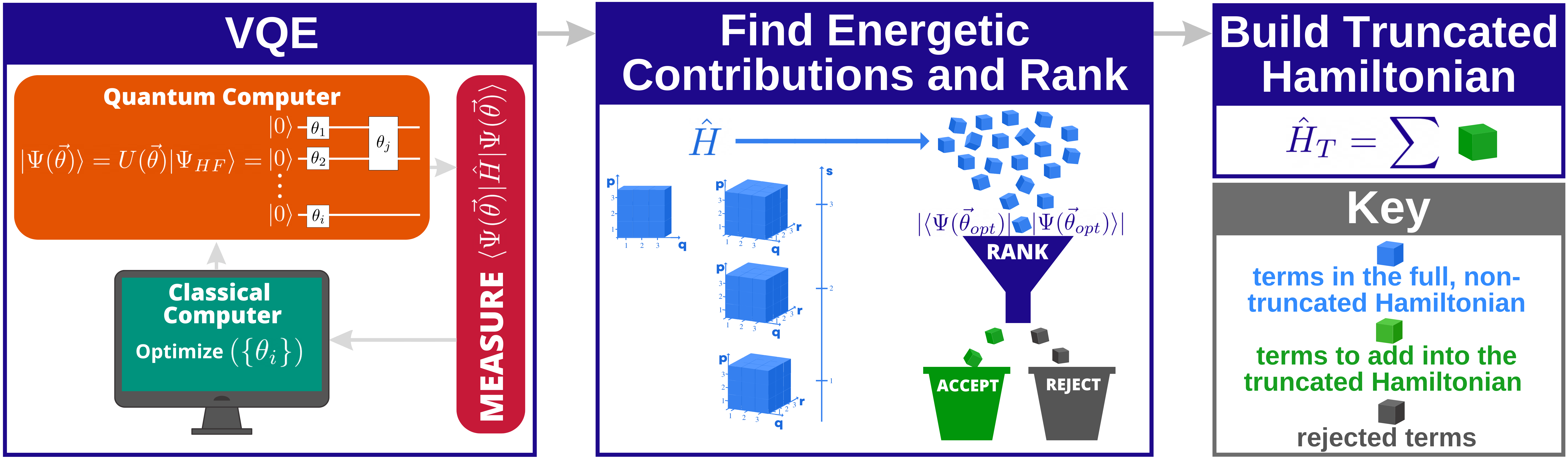
Figure 2: A schematic diagram of the non-iterative truncation with VQE using the energetic ranking scheme. Each cube represents one Hamiltonian term. The first panel shows the calculation of the optimized ansatz, $\Psi(\vec{\theta}_{opt})$, using VQE. The next panel illustrates the ranking of the terms using $\Psi(\vec{\theta}_{opt})$. The last panel shows the truncated Hamiltonian as a sum of the most important terms.

While Benchmark 1 is useful, it can be improved in practice by making use of the variational principle. We refer to this benchmark as Benchmark 2. Without changing the ranking in Step 4, we can calculate the following energy:

$$E_{T,\text{ v}}^{k}=\expectationvalue{\hat{H}}{\Psi_{T,0}^{k}}.$$ (11)

We expect a faster convergence when Eqn. (11) is used in Step 2 since it uses the full Hamiltonian to calculate the expectation value. However, there is a trade-off between accuracy and the number of measurements one would need to make on a quantum computer when using the full Hamiltonian in place of the truncated Hamiltonian to calculate the energy.

III.5 Energy estimates using classical shadows

In each iteration $k$ of SQuISH, we have a state $\ket{\Psi_{T,0}^{k}}$ and need estimates of both the total energy $E_{T}^{k}$ (using the current truncated Hamiltonian) and the energetic contributions of the remaining one- and two-body terms (indexed by $\mathbb{T}^{k}$). These can be calculated from estimates of all of the 2-RDMs. The state of the art for estimating all 2-RDMs is based on classical shadows. In the general framework for partial tomography using classical shadows, a Positive Operator Valued Measure (POVM) is chosen such that $l$ observables ${\left(\hat{O}_{i}\right)}_{i=1}^{l}$ from a given family can be estimated to within $\epsilon$ additive error using $O\left(\log l\max_{i}{\left\|{\hat{O}_{i}}\right\|}_{\mathrm{shadow}}/\epsilon^{2}\right)$ of the POVM Huang et al. (2020); Elben et al. (2022), where ${\left\|\cdot\right\|}_{\mathrm{shadow}}$ is a POVM-specific norm related to the variance of the estimator. The POVM is typically specified using an ensemble of unitaries such that the POVM results from choosing a unitary uniformly at random from the ensemble and then measuring in the computational basis. The choice of POVM depends on the type of observable to be estimated, but not on the specific observables once the type is fixed. Several recent works have developed protocols for measuring fermionic observables using classical shadows Zhao et al. (2021); Wan et al. (2022); O’Gorman (2022); Low (2022). In particular, Low showed that when the state to be measured has a fixed number $\eta$ of electrons, all of the 2-RDMs can be estimated to within additive error $\epsilon$ using only

$$\binom{\eta}{2}{\left(1-\frac{\eta-2}{N}\right)}^{2}\frac{N+1}{N-1}\frac{1}{\epsilon^{2}}$$ (12)

measurements Low (2022). The ensemble of unitaries used is simply Haar-random single-particle basis changes, which can be implemented in linear depth with linear connectivity (when using the Jordan-Wigner encoding) Jiang et al. (2018). Computing the estimates of the RDMs given the sampled unitaries and measurement outcomes can be done efficiently. Furthermore, because the measurements are non-adaptive, the estimation procedure can be trivially parallelized.

In theory, there may be a more efficient measurement protocol for the observables of interest (the total energy and energetic contributions) that exploits some structure in the observables. However, because we are focused on sparse truncations of the Hamiltonian terms, the excluded terms indexed by $\mathbb{T}^{k}$ can include almost all of the terms, and so we essentially need to measure all of the 2-RDMs anyway. That being said, each energetic contribution has a coefficient $h_{pqrs}$ that is not taken into account in the scheme based on classical shadows; there is potential there for improving the measurement efficiency, which we leave to future work.

IV Extensions of SQuISH

By adopting and expanding upon some of the methods proposed in Section III, one can develop useful variations of SQuISH. There are a multitude of SQuISH extensions, which can be explored in future work, but here we will discuss two such extensions. While we largely focus on Hamiltonian truncation for ground state problems in this paper, SQuISH can also be employed for excited state calculations by slightly altering our algorithm. We call this modified algorithm ”multi-reference SQuISH” and explain the details. Additionally, our energetic ranking scheme without the iterative portion of SQuISH may be of interest. We discuss a method of using an approximate wavefunction to rank terms and truncate a Hamiltonian non-iteratively.

IV.1 Multi-reference SQuISH

If one is interested in truncating a Hamiltonian for dynamics, considering excited states might be useful to create a selected energy space for the dynamics and can be included in the truncation process. We can create a multi-reference version of SQuISH such that it includes terms based on both ground and excited state energetic contributions. In Step 2, we can calculate the $J$ truncated Hamiltonian wavefunctions of interest, such as $\{\ket{\Psi_{T,0}^{k}},\ket{\Psi_{T,1}^{k}},\ket{\Psi_{T,2}^{k}},\dots\ket{\Psi_{T,J}^{k}}\}$. Then in Step 4, we would calculate the energetic contributions of the terms with each of the $J$ wavefunctions as follows:

$$\begin{gathered}\left\{\epsilon_{i,0}=\begin{cases}\expectationvalue{h_{pq}\hat{a}_{p}^{\dagger}\hat{a}_{q}+h.c.}{\Psi_{T,0}^{k}}\\ \expectationvalue{h_{pqrs}\hat{a}_{p}^{\dagger}\hat{a}_{q}^{\dagger}\hat{a}_{r}\hat{a}_{s}+h.c.}{\Psi_{T,0}^{k}}\end{cases}\right\}\\ \left\{\epsilon_{i,1}=\begin{cases}\expectationvalue{h_{pq}\hat{a}_{p}^{\dagger}\hat{a}_{q}+h.c.}{\Psi_{T,1}^{k}}\\ \expectationvalue{h_{pqrs}\hat{a}_{p}^{\dagger}\hat{a}_{q}^{\dagger}\hat{a}_{r}\hat{a}_{s}+h.c.}{\Psi_{T,1}^{k}}\end{cases}\right\}\\ \left\{\epsilon_{i,2}=\begin{cases}\expectationvalue{h_{pq}\hat{a}_{p}^{\dagger}\hat{a}_{q}+h.c.}{\Psi_{T,2}^{k}}\\ \expectationvalue{h_{pqrs}\hat{a}_{p}^{\dagger}\hat{a}_{q}^{\dagger}\hat{a}_{r}\hat{a}_{s}+h.c.}{\Psi_{T,2}^{k}}\end{cases}\right\}\\ \vdots\\ \left\{\epsilon_{i,J}=\begin{cases}\expectationvalue{h_{pq}\hat{a}_{p}^{\dagger}\hat{a}_{q}+h.c.}{\Psi_{T,J}^{k}}\\ \expectationvalue{h_{pqrs}\hat{a}_{p}^{\dagger}\hat{a}_{q}^{\dagger}\hat{a}_{r}\hat{a}_{s}+h.c.}{\Psi_{T,J}^{k}}\end{cases}\right\}.\end{gathered}$$ (13)

After ranking each set of energetic contributions in Step 5, we can update the Hamiltonian with $m$ terms consisting of the $m/J$ most important terms from each set. Convergence criteria can be extended to include the convergence of the excited states in the loss function.

IV.2 Non-Iterative Truncation with VQE

Algorithms like VQE can be used in combination with the energetic ranking scheme to truncate the Hamiltonian non-iteratively. SQuISH is reliant on an iteratively updated trial wavefunction to rank terms. However, a one-shot approach for the compression process may be useful in practice. We can build the truncated Hamiltonian all in one iteration by using a sufficiently accurate wavefunction to rank all terms. One can use VQE to optimize a Unitary Coupled Cluster (UCC) ansatz Bartlett et al. (1989); Hoffmann and Simons (1988), a Hamiltonian variational ansatz (HVA) Wecker et al. (2015), or a hardware-efficient ansatz Kandala et al. (2017) in place of the iteratively updated SQuISH trial wavefunction to determine which Hamiltonian terms to exclude from the truncated Hamiltonian. A schematic diagram of this process is shown in Fig. 2.

A non-iteratively truncated Hamiltonian may be utilized both to study dynamics and find more accurate ground state solutions. We expect that in some cases an optimized trial VQE wavefunctions generated without necessarily reaching chemical accuracy can be sufficiently good for finding the energetic contributions of terms and ranking. Once the truncated Hamiltonian is built, one can use QPE or other approaches to calculate the energy. In that case, the non-iterative truncation process is not only useful for building a resource-efficient Hamiltonian to simulate dynamics, but it is also beneficial for ground state calculations if the goal is a chemically accurate energy.

V Simulation Details

Molecule	N${}_{\text{O}}$	N${}_{\text{V}}$	Qubits	one-body terms	two-body terms	terms in $\mathbb{I}^{0}$	terms in $\mathbb{T}^{0}$	$vvvv$ terms variational SQuISH	$vvvv$ terms non-variational SQuISH
NH3 (cc-pVTZ)	5	67	144	$5.18\text{\times}{10}^{3}$	$2.69\text{\times}{10}^{7}$	$6.72\text{\times}{10}^{6}$	$2.02\text{\times}{10}^{7}$	$1.93\text{\times}{10}^{5}$	$2.11\text{\times}{10}^{6}$
HF (cc-pVQZ)	5	80	170	$7.23\text{\times}{10}^{3}$	$5.22\text{\times}{10}^{7}$	$1.12\text{\times}{10}^{7}$	$4.70\text{\times}{10}^{7}$	$3.28\text{\times}{10}^{4}$	$1.12\text{\times}{10}^{6}$
LiH (cc-pVQZ)	2	83	170	$7.23\text{\times}{10}^{3}$	$5.22\text{\times}{10}^{7}$	$4.74\text{\times}{10}^{6}$	$4.75\text{\times}{10}^{7}$	$1.91\text{\times}{10}^{4}$	$2.25\text{\times}{10}^{5}$
F2 (cc-pVQZ)	9	101	220	$1.21\text{\times}{10}^{4}$	$1.46\text{\times}{10}^{8}$	$4.23\text{\times}{10}^{7}$	$1.04\text{\times}{10}^{8}$	$1.93\text{\times}{10}^{5}$	$2.17\text{\times}{10}^{6}$
C2 (cc-pVQZ)	6	104	220	$1.21\text{\times}{10}^{4}$	$1.46\text{\times}{10}^{8}$	$2.94\text{\times}{10}^{7}$	$1.17\text{\times}{10}^{8}$	$2.05\text{\times}{10}^{5}$	$2.29\text{\times}{10}^{6}$
H2 (cc-pV5Z)	1	109	220	$1.21\text{\times}{10}^{4}$	$1.46\text{\times}{10}^{8}$	$5.25\text{\times}{10}^{6}$	$1.41\text{\times}{10}^{8}$	$4.2\text{\times}{10}^{3}$	$2.26\text{\times}{10}^{4}$
H2O (cc-pVQZ)	5	110	230	$1.32\text{\times}{10}^{4}$	$1.75\text{\times}{10}^{8}$	$2.85\text{\times}{10}^{7}$	$1.46\text{\times}{10}^{8}$	$3.62\text{\times}{10}^{5}$	$5.70\text{\times}{10}^{6}$
BeH2 (cc-pVQZ)	3	112	230	$1.32\text{\times}{10}^{4}$	$1.74\text{\times}{10}^{8}$	$1.75\text{\times}{10}^{7}$	$1.57\text{\times}{10}^{8}$	$4.04\text{\times}{10}^{4}$	$3.97\text{\times}{10}^{5}$

Table 2: This table shows the data for coupled cluster variational and non-variational SQuISH tests using PyCC. The N${}_{\text{O}}$ and N${}_{\text{V}}$ columns show the number of occupied and virtual spatial orbitals, respectively. The qubits column shows the number of qubits required to simulate the molecule on a quantum computer. The one- and two-body terms columns show how many total terms are in $\hat{H}$. The terms in $\mathbb{I}^{0}$ column shows the number of ERI terms in the initial truncated Hamiltonian, and the terms in $\mathbb{T}^{0}$ column shows the number of terms in $\hat{H}-\hat{H}_{T}$. The variational and non-variational SQuISH columns illustrate the number of $vvvv$ needed to achieve chemical accuracy. We use Feller geometries for H₂O, HF, NH₃ F₂, and LiH, and we use NIST calculated geometries at equilibrium for $\ce{C2}$, $\ce{H2}$, and $\ce{BeH2}$ Feller et al. (2008); Johnson (1999).

We generate ground state wavefunctions using configuration interaction for systems on the order of 10 qubits and coupled cluster for systems that would require on the order of 100+ qubits to test our approach. These simulations serve as a test bed for the performance we can expect to achieve in practice with regard to the compression of a Hamiltonian. In practice, various methods could be used to generate the iterative wavefunction during the SQuISH algorithm, such as time evolution, phase estimation, adiabatic state preparation Alán et al. (2005); Crosson and Lidar (2021); Hauke et al. (2020); Brady et al. (2021); Kremenetski et al. (2021a), and QAOA Kremenetski et al. (2021b).

As we consider larger basis sets, the virtual space dominates. The majority of the terms in the Hamiltonian come from the two-body virtual terms. Thus, we chose the initial Hamiltonian such that it includes all terms except two-body virtual terms in Step 1. The initial Hamiltonian, $\hat{H}_{T}^{0}$, is defined using the initial set of terms shown below,

$$\begin{split}&\mathbb{I}^{0}=\{(p,q)\}\cup\\ &\{(p,q,r,s):(p,q,r,s)\notin\{(v,v,v,v)\}\}.\end{split}$$ (14)

Here, $v$ denotes the virtual orbitals. Similar to the two benchmarks described in the previous section, in Step 2 we have the option of calculating the energy non-variationally (i.e., Eqn. (10)) or variationally (i.e., Eqn. (11)). We implement and compare both non-variational and variational SQuISH.

We use PyCC Crawford (2021) to run coupled cluster and calculate the energy for the truncated Hamiltonians with our method. During this approach, we also generate the density matrices used for the ranking and energy calculations. The ranking equations are based on the reduced density matrices (Eqns. 5 and 6). The non-variational energy is calculated with only the subset of terms included in the truncated Hamiltonian,

$$E_{CCSD_{T,{\text{nv}}}}^{k}=\sum_{p,q}h_{pq}\gamma_{p,q}+\sum_{p,q,r,s\in\mathbb{I}^{k}}h_{pqrs}\Gamma_{p,q,r,s}^{k}.$$ (15)

As mentioned above, one can calculate a variational energy, with respect to the full Hamiltonian, even when using the ground state of the truncated Hamiltonian. We modify the summation to include all of the elements in $\hat{H}$, not just $\hat{H}_{T}$

$$E_{CCSD_{T,{\text{v}}}}^{k}=\sum_{p,q}h_{pq}\gamma_{p,q}+\sum_{p,q,r,s}h_{pqrs}\Gamma_{p,q,r,s}^{k}.$$ (16)

We note that while in practice, the SQuISH termination condition in Step 3 is based on the error calculated using the energy from the previous iteration (i.e., $\absolutevalue{E_{T}^{k-1}-E_{T}^{k}}$), we use the exact energy (i.e., $\absolutevalue{E_{0}-E_{T}^{k}}$) for testing purposes.

In Step 4, we calculate the energetic importance of each term in $\mathbb{T}^{k}$ using the 2RDMs

$$\epsilon_{i}=h_{pqrs}\Gamma_{p,q,r,s}^{k}\text{ for $(p,q,r,s)\in\mathbb{T}^{k}$}.$$ (17)

We rank the terms using Eqn. (17) based on the energetic contribution in Step 5. In Step 6, we start with a small $m$ with respect to system size and, after the first iteration, continually increase it by an order of magnitude every few iterations.

For small systems, we test SQuISH using Qiskit et al. (2021) with configuration interaction, which is an exact method (unlike coupled cluster). Due to current limitations, we use small systems to do the configuration interaction truncation. The molecules we use to perform our calculations require 12 qubits. As a result, the truncation space is relatively small.

VI Results and Discussion

VI.1 Coupled Cluster Results

Molecule	N${}_{\text{O}}$	N${}_{\text{V}}$	one-body terms	two-body terms	terms in $\mathbb{I}^{0}$	terms in $\mathbb{T}^{0}$	$vvvv$ terms variational SQuISH	$vvvv$ terms non-variational SQuISH	$\absolutevalue{\bra{\Psi_{T,0}^{k}}\ket{\Psi_{0}}}$
H2 (cc-pVDZ)	1	5	36	1,296	671	625	6	55	0.99951506
H3+ (cc-pVDZ)	1	5	36	1,296	671	625	16	33	0.99974916
LiH (STO-3G)	2	4	36	1,296	1040	256	10	10	0.99990412

Table 3: This table provides data from the variational and non-variational SQuISH tests using Qiskit. The N${}_{\text{O}}$ and N${}_{\text{V}}$ columns show the number of occupied and virtual spatial orbitals, respectively. The one- and two-body terms columns show how many total terms are in $\hat{H}$. The $\mathbb{I}^{0}$ column shows the number of ERI terms in the initial truncated Hamiltonian, and the $\mathbb{T}^{0}$ column shows the number of terms in $\hat{H}-\hat{H}_{T}$. The variational and non-variational SQuISH columns show how many $vvvv$ ERI terms are needed to achieve chemical accuracy after applying SQuISH. The last column shows the overlap between the accurate ground state wavefunction and the ground state wavefunction of the variational SQuISH truncated Hamiltonian at chemical accuracy. For each molecule, we use the equilibrium calculated geometries from NIST Johnson (1999).

We use variational and non-variational SQuISH with coupled cluster states to truncate the Hamiltonians of the following systems: HF, LiH, F₂, C₂, H₂O and BeH₂ in the cc-pVQZ basis, NH₃ in the cc-pPVTZ basis, and H₂ in the cc-pV5Z basis. For each molecule, we evaluate the number of two-body virtual terms that need to be included in the truncated Hamiltonian to reach chemical accuracy after applying SQuISH. Table 2 contains the data illustrating the total number of terms in each Hamiltonian and the number of terms after applying the SQuISH algorithm. The number of terms is reduced by between two to five orders of magnitude after applying SQuISH. We also see that calculating the energy variationally improves the truncation by at least an order of magnitude.

SQuISH not only reduces the number of Hamiltonian terms but can also have a favorable effect on the Hamiltonian norm, with different norms yielding resource estimates for different algorithms Childs et al. (2021a). Such norms commonly arising in matrix analysis can often be bounded in terms of each other. Here we consider the sum of the absolute values of the Hamiltonian coefficients as an indicative quantity, i.e., the 1-norm of the vector of coefficients, which we denote as

$${|\kern-1.07639pt|\kern-1.07639pt|\hat{H}|\kern-1.07639pt|\kern-1.07639pt|}_{1}:=\sum_{p,q}\absolutevalue{h_{pq}}+\frac{1}{2}\sum_{p,q,r,s}\absolutevalue{h_{pqrs}}.$$ (18)

This quantity is used in the calculations shown in Table 4. We calculate and compare it for the non-truncated Hamiltonians, the chemically accurate SQuISH truncated Hamiltonians, and the coefficient ranking truncated Hamiltonians.

Molecule	${{|\kern-1.07639pt|\kern-1.07639pt|\hat{H}|\kern-1.07639pt|\kern-1.07639pt|}}_{1}$	SQuISH ${{|\kern-1.07639pt|\kern-1.07639pt|\hat{H}_{T}|\kern-1.07639pt|\kern-1.07639pt|}}_{1}$	Coefficient Ranking ${{|\kern-1.07639pt|\kern-1.07639pt|\hat{H}_{T}|\kern-1.07639pt|\kern-1.07639pt|}}_{1}$
NH3 (cc-pVTZ)	$3.26\text{\times}{10}^{4}$	$1.18\text{\times}{10}^{4}$	$2.18\text{\times}{10}^{4}$
HF (cc-pVQZ)	$4.57\text{\times}{10}^{4}$	$1.81\text{\times}{10}^{4}$	$2.35\text{\times}{10}^{4}$
LiH (cc-pVQZ)	$1.65\text{\times}{10}^{4}$	$2.15\text{\times}{10}^{3}$	$7.40\text{\times}{10}^{3}$
F2 (cc-pVQZ)	$7.91\text{\times}{10}^{4}$	$3.36\text{\times}{10}^{4}$	$5.54\text{\times}{10}^{4}$
C2 (cc-pVQZ)	$5.66\text{\times}{10}^{4}$	$1.92\text{\times}{10}^{4}$	$3.90\text{\times}{10}^{4}$
H2 (cc-pV5Z)	$7.25\text{\times}{10}^{4}$	$4.28\text{\times}{10}^{3}$	$2.10\text{\times}{10}^{4}$
H2O (cc-pVQZ)	$1.01\text{\times}{10}^{5}$	$2.71\text{\times}{10}^{4}$	$5.45\text{\times}{10}^{4}$
BeH2 (cc-pVQZ)	$4.88\text{\times}{10}^{4}$	$8.16\text{\times}{10}^{3}$	$2.71\text{\times}{10}^{4}$

Table 4: This table shows the one norms of the full and truncated Hamiltonians of each molecule tested. ${|\kern-0.96873pt|\kern-0.96873pt|\hat{H}_{T}|\kern-0.96873pt|\kern-0.96873pt|}_{1}$ is calculated for both SQuISH and the coefficient ranking scheme truncation once chemical accuracy is reached.

Fig. 3 presents more detailed results at each iteration using coupled cluster calculations for H₂O in the cc-pVQZ basis. We use the energy and error plots to evaluate the two benchmark comparisons, variational SQuISH, and non-variational SQuISH using the $\ce{H2O}$ data. Considering Fig. 3(a), we see that Benchmark 1 and Benchmark 2 almost completely overlap variational SQuISH and non-variational SQuISH, respectively. This implies that using an approximate wavefunction for the ranking is nearly as good as using the exact wavefunction.

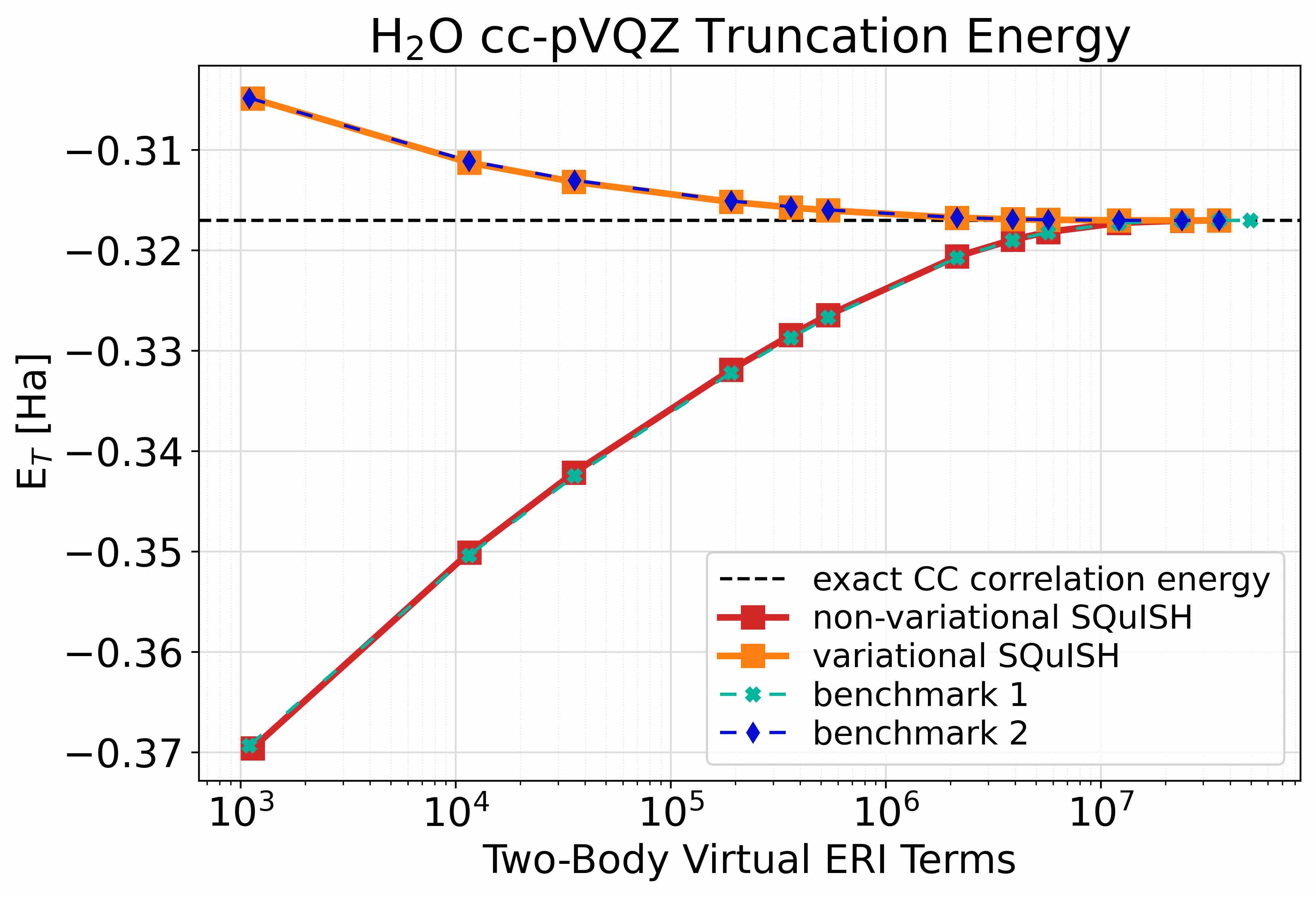
(a) Semi-logarithmic energy plot

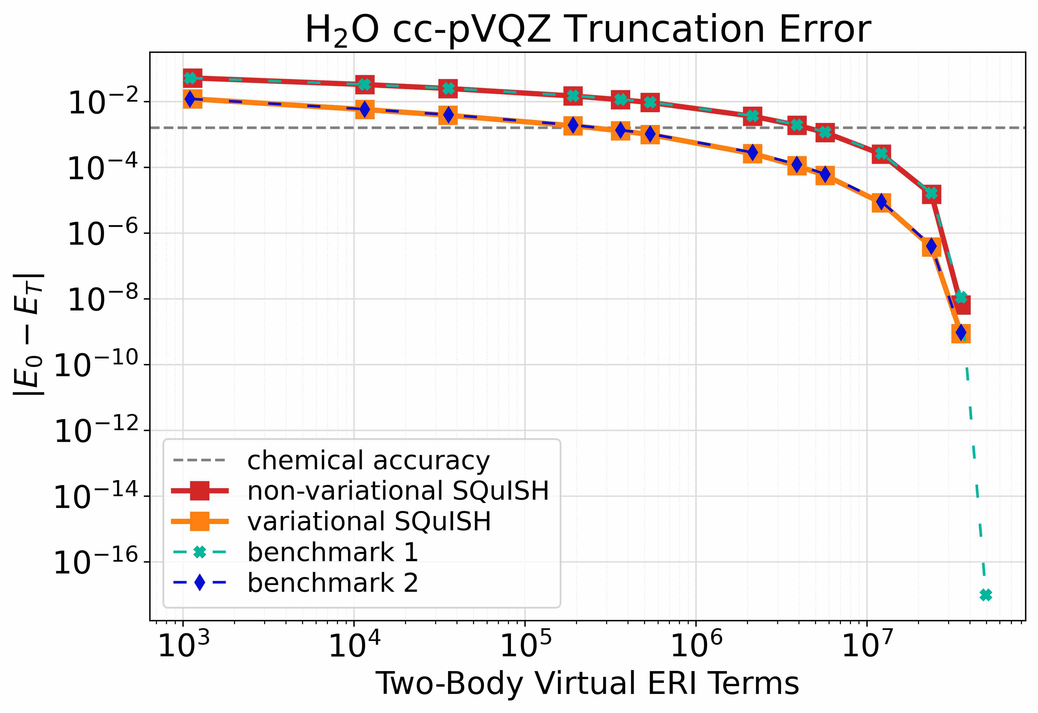
(b) Semi-logarithmic error plot

Figure 3: Coupled-cluster H2O in the cc-pVQZ basis. The energy on the plots is the coupled cluster correlation energy. Each point on the plots represents one self-consistent iteration. SQuISH and the benchmarks terminate once the approximate energy is within $1\text{\times}{10}^{-8}$ Hartrees of the exact energy.

The high accuracy we get from our approximate Hamiltonians and approximate wavefunctions is not surprising given that classical methods have shown similar convergence properties in slightly different contexts, such as the ASCI algorithm Tubman et al. (2016). Given SQuISH behaves so similarly to the benchmarks, we conclude that $\ket{\Psi_{T,0}^{k}}$ contains enough information at each step to find the next set of important terms to add in the Hamiltonian.

The results exemplify the advantage in calculating the energy variationally. However, there is a trade-off between a faster convergence and the number of measurements. If the energy is calculated non-variationally and we use previously discussed techniques, such as shadow tomography, in Step 4, we can reduce the number of measurements we need to make on a quantum computer in exchange for accuracy.

VI.2 Configuration Interaction Results

We test variational and non-variational SQuISH for H2, H3+, LiH for various basis sets using Qiskit. Table 3 illustrates how many terms are required to achieve chemical accuracy for the molecules tested.

We use full configuration interaction for LiH in the STO-3G basis and truncate H2 and H3+ to 6 spacial orbitals in the cc-pVDZ basis. Although the number of ERIs are fairly small, we still substantially truncate the number of terms after applying SQuISH. The variational truncation slightly outperforms the non-variational truncation when applied to H2 and H3+, and they perform about the same when applied to LiH. The advantage of variational SQuISH is reduced here in comparison to the coupled cluster results because we are using very small systems. We include results showing the wavefunction overlap once the ground state energy is within chemical accuracy. Additionally, we test the non-iterative truncation with VQE using a UCC with singles and doubles (UCCSD) ansatz on the H2 Hamiltonian.

As a direct comparison, we test SQuISH using $\ce{LiH}$ in the STO-3G basis for coupled cluster and full configuration interaction. A main goal here is to show that the approximations from coupled cluster do not significantly change from what can be expected from a quantum computer, which is closely represented by the configuration interaction results. Our results, in Fig. 4, do indeed look very similar between the two approaches, which gives us confidence that our coupled cluster results (in Section VI.1) for larger systems reasonably demonstrate how well the SQuISH compression technique works on larger Hamiltonians. For comparisons between accurate configuration interaction and coupled cluster simulations, see Tubman et al. (2018).

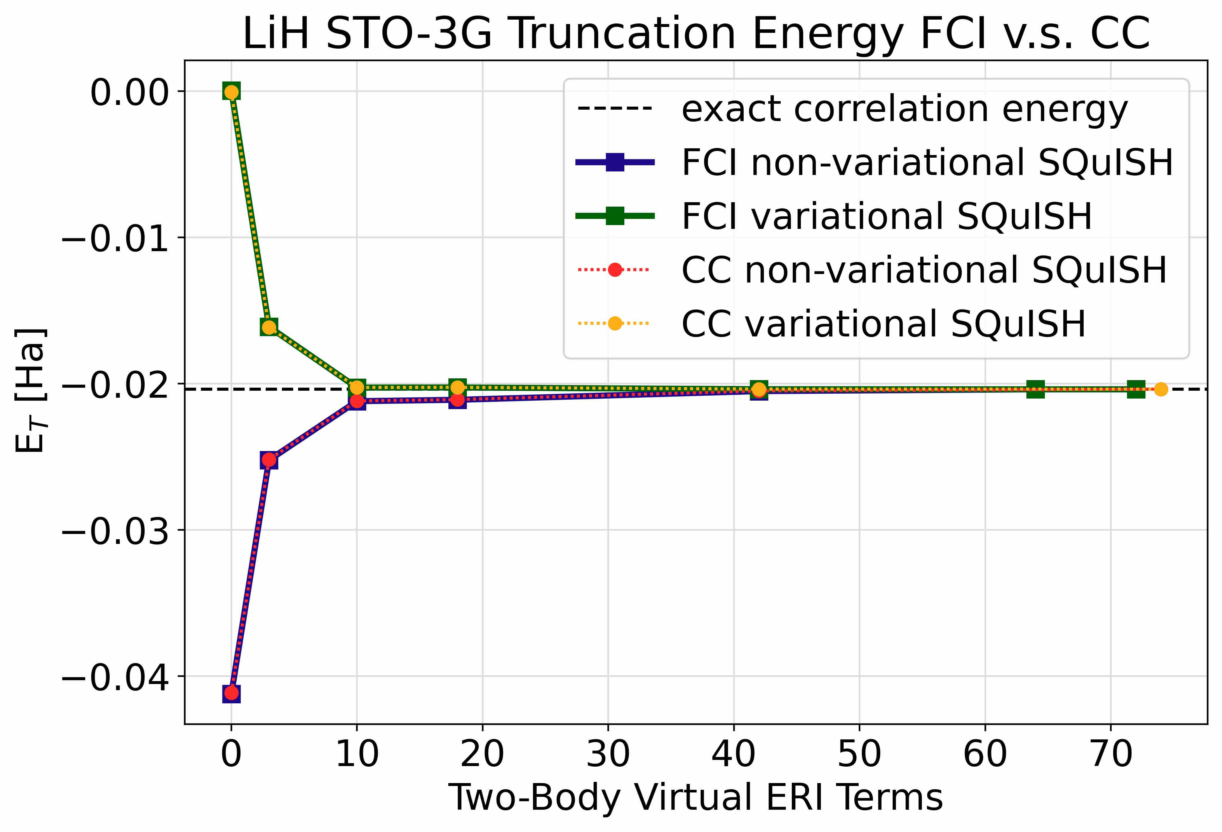
(a) Energy plot

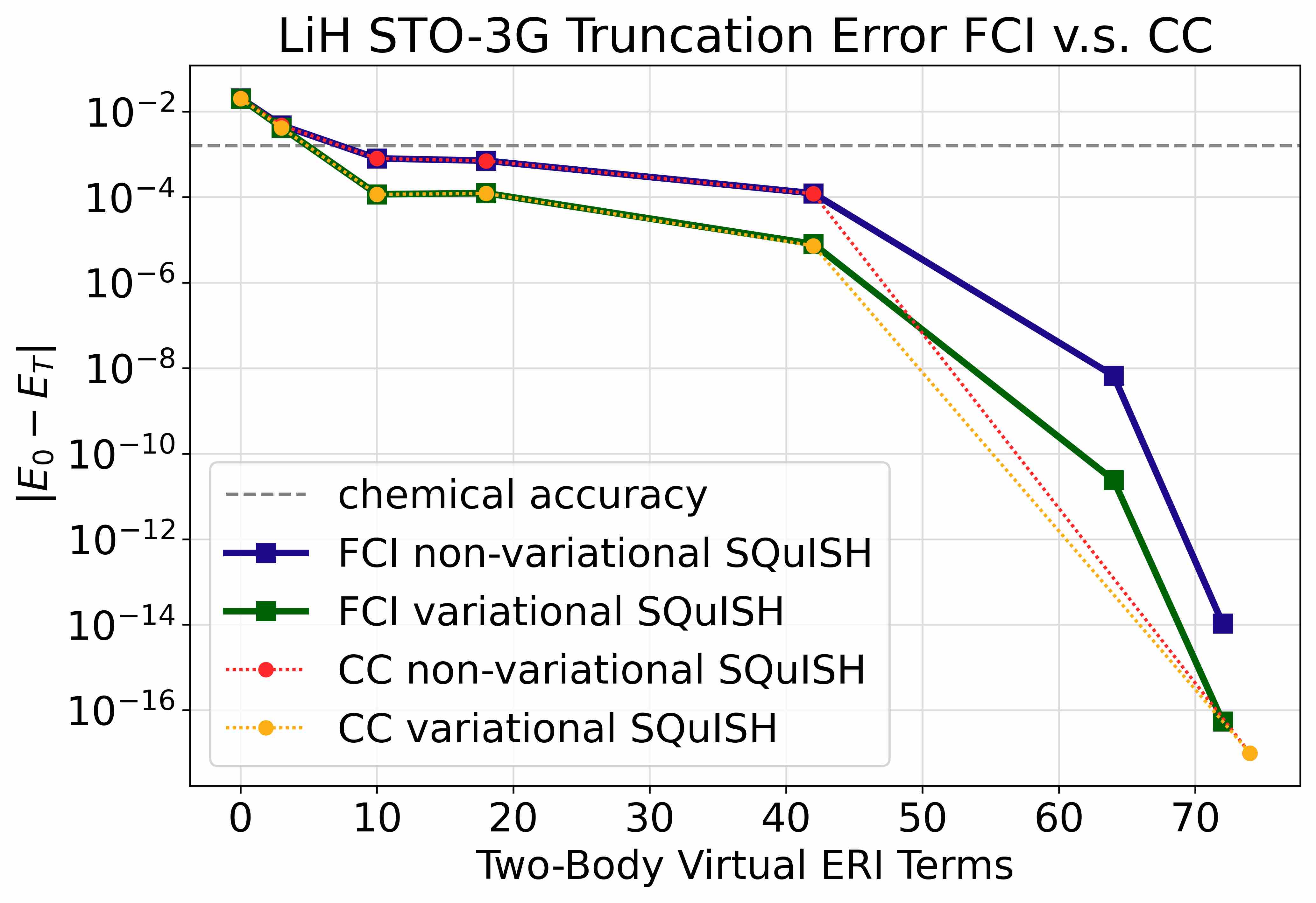
(b) Error plot

Figure 4: A comparison of the full configuration interaction and coupled cluster tests of SQuISH using LiH in the STO-3g basis. The dark green and light orange compare the variational results. The dark blue and light red lines compare the non-variational results. We plot the correlation energy. SQuISH and the benchmarks terminate once the approximate energy is within $1\text{\times}{10}^{-12}$ Ha of the exact energy.

The results of the non-iterative truncation are shown in Fig. 5. We test it on the H2 Hamiltonian by first optimizing a parameterized UCCSD ansatz with VQE to an accuracy of $2.02\text{\times}{10}^{-2}$, which is above chemical accuracy. Then we rank terms based on energetic contributions and build the truncated Hamiltonian. We also compare against the coefficient ranking, in which we determine importance based on $\absolutevalue{h_{pqrs}}$. For both of these methods, we use the exact ground state wavefunction to calculate the energy at the end (i.e., $\expectationvalue{\hat{H}_{T}}{\Psi_{0}})$. We also add non-variational SQuISH to the plot as a comparison metric.

The non-iterative truncation with the energetic ranking performs fairly similarly to SQuISH. As we expected, the VQE trial wavefunction performed well when calculating the energetic contributions even though we terminated VQE prior to achieving a chemically accurate solution. Moreover, the fact that both SQuISH and the energetic ranking non-iterative truncation outperform the coefficient ranking truncation further validates the argument for an energetic ranking scheme.

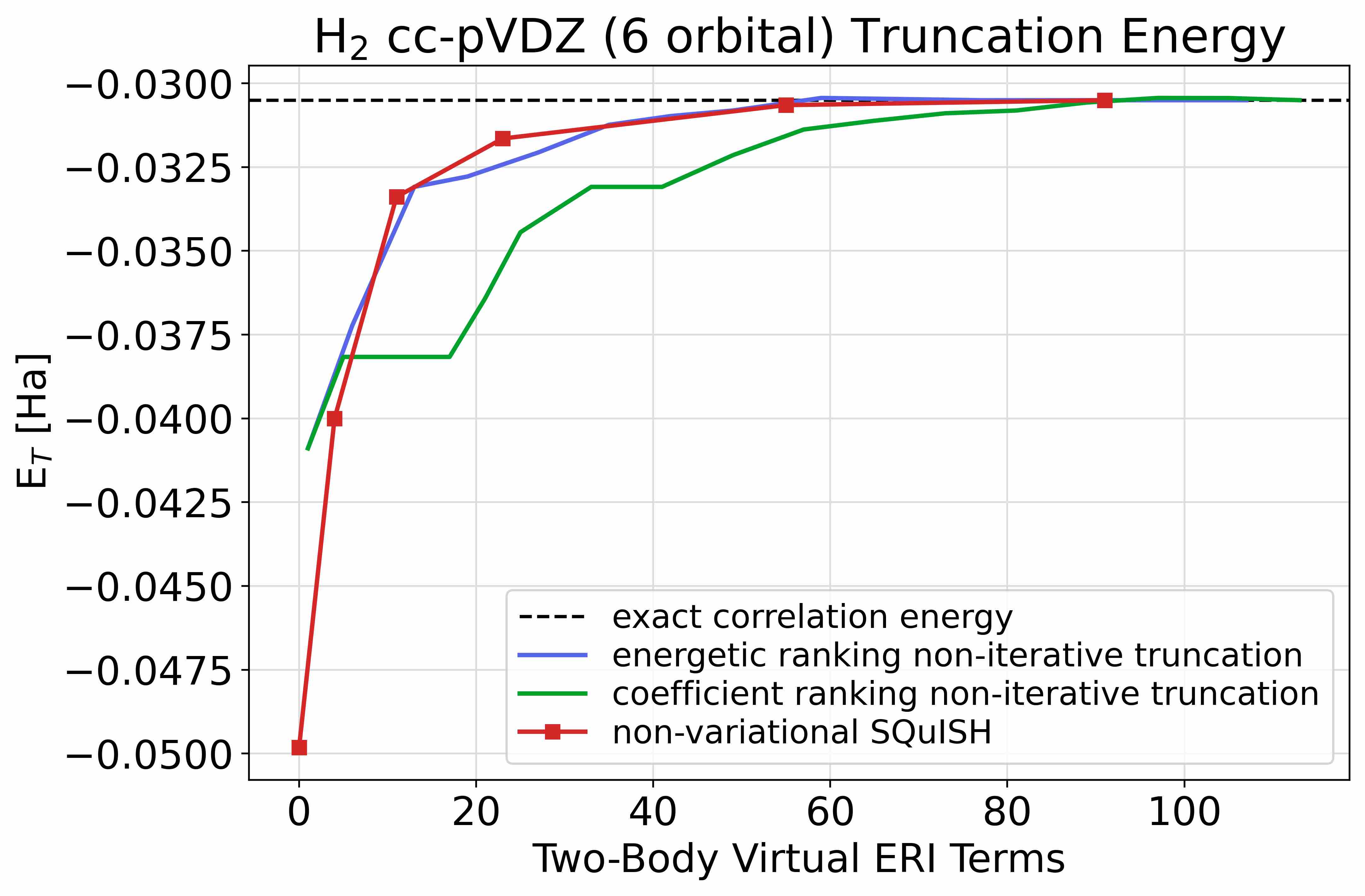
(a) Energy plot

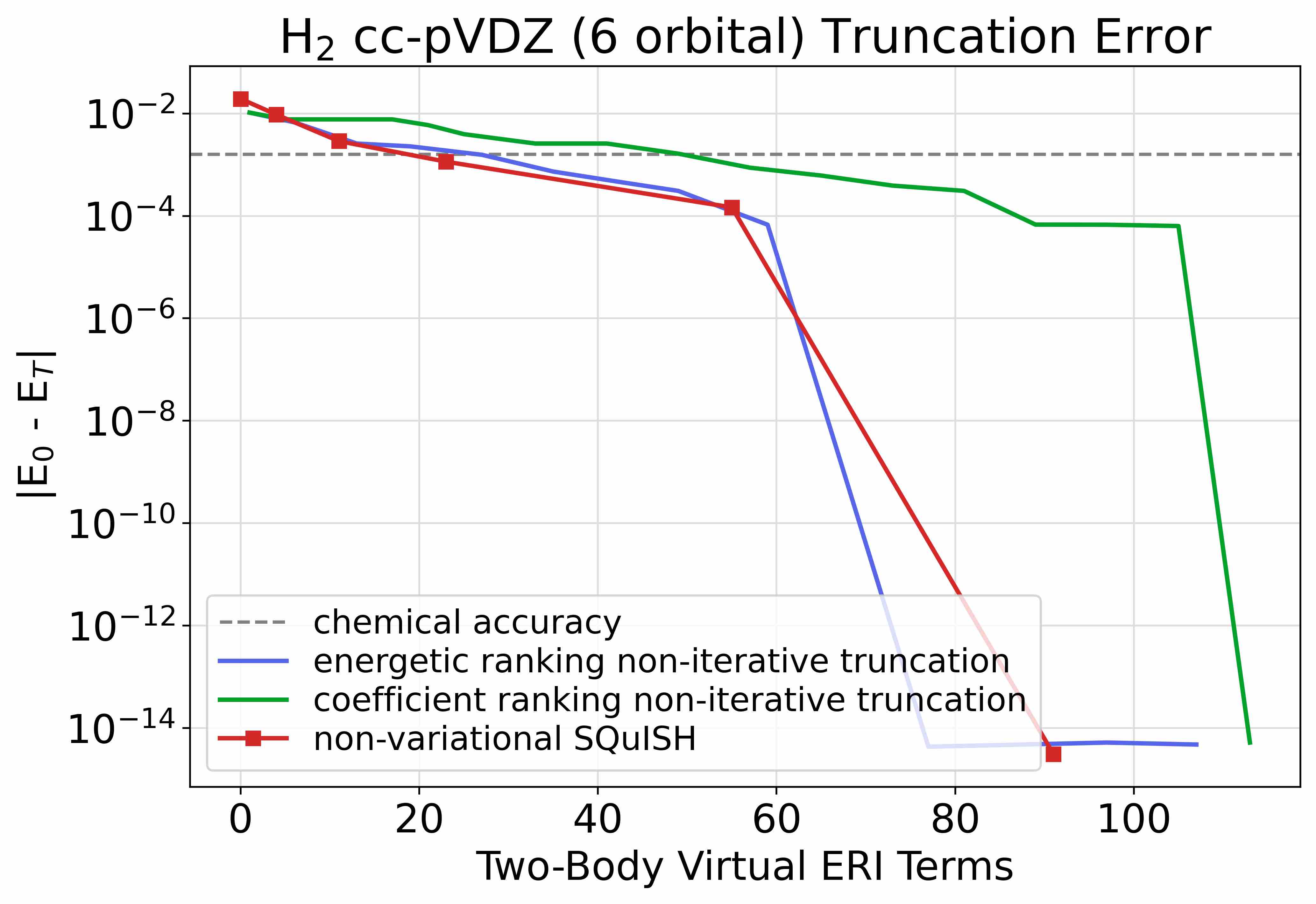
(b) Error plot

Figure 5: A comparison of non-iterative truncation using VQE and non-variational SQuISH using 6 orbital H2 in the cc-pVDZ basis. The purple line shows the use of the energetic ranking scheme with an optimized UCCSD ansatz. The green line shows the coefficient ranking scheme. The red line shows non-variational SQuISH, where each point represents one self-consistent iteration.

VI.3 Energetic versus Coefficient Ranking

Here we will provide data to support the claim that ranking Hamiltonian terms based on energetic contributions is better than ranking based on the value of the Hamiltonian coefficients alone. We use coupled cluster states with Benchmark 1 for the comparison.

(a) A semi-logarithmic plot of the number of two-body virtual terms included in the truncated Hamiltonian at each iteration versus the approximate coupled cluster correlation energy.

(b) Semi logarithmic plot of the number of two-body virtual terms versus the absolute value of approximate energy error near chemical accuracy.

Figure 6: Energetic ranking scheme versus coefficient ranking scheme using coupled cluster Benchmark 1 with H₂O in the cc-pVQZ basis. The algorithm terminates once the energy is within $1\text{\times}{10}^{-8}$ of the accurate energy.

For each approach, we initialize the truncated Hamiltonian with Eqn. (14), calculate the energies variationally, and check for convergence in Step 3. The difference between these tests occurs in Steps 4 and 5. For the coefficient ranking, we have nothing to calculate in Step 4, as we have all the coefficients for the Hamiltonian already calculated. In Step 5 we rank the terms, $h_{pqrs}\hat{a}_{p}^{\dagger}\hat{a}_{q}^{\dagger}\hat{a}_{r}\hat{a}_{s}$, based on absolute value of the coefficients, $\absolutevalue{h_{pqrs}}$.

We test the two ranking methods here using H₂O in the cc-pVQZ basis. The significant advantage we gain by using the expectation value ranking is evident in Fig. 6. Fig. 6(b) shows the few SQuISH iterations before and after the energy converges to chemical accuracy. One can see that the energetic ranking requires an order of magnitude fewer terms compared to coefficient ranking to reach a chemically accurate solution. For larger systems, we expect our approach to lead to even more substantial reductions.

VII Conclusion and Outlook

The field of quantum computing has seen an extensive number of proposed approaches to reduce the Hamiltonian complexity with the intention of making time evolution and related approaches feasible using fewer quantum resources. While the goal of this work is the same, we take a new approach to accomplish this task that makes use of information from an iteratively improved approximate wavefunction, something that takes advantage of the unique capabilities of quantum computers and has not been used in previous algorithms to our knowledge. Using the SQuISH algorithm, we show that this information is, in fact, a key ingredient to creating a compression algorithm, and we demonstrate this on a series of chemistry Hamiltonians. The idea that different eigenstates will be sensitive to different terms in the Hamiltonian is evident, and the key proposal in our algorithm is that an approximate trial wavefunction can be good enough to provide improved convergence over canonical approaches.

Our proposal leads to several expected uses. First, we note that although we are hopeful that our compression scheme will be especially advantageous in the NISQ era, quantum advantage, it will also be useful in the long term on fault-tolerant hardware. The idea that we will run arbitrarily large circuits on fault-tolerant hardware is incorrect, as algorithms can still take days/weeks/months to run, even if they have polynomial scaling. Thus compressing a Hamiltonian, which can grow to many gigabytes of memory on classical hardware, will undoubtedly be beneficial in the near term and fault-tolerant era. We also want to emphasize that our compression scheme is unique and complementary to a large number of other compression techniques. By using the information in the wavefunction, one can pick out better terms to include in the Hamiltonian for other compression schemes as well. Thus our method complements other approaches, and we expect this will push us closer to finding a path to quantum advantage for quantum chemistry.

There are several directions for future work to either improve SQuISH or integrate it into various quantum algorithms, including potential applications beyond chemistry. To further reduce the complexity of a Hamiltonian, one can explore the best terms to include in the initial Hamiltonian. Additionally, by refining the algorithm to incorporate state-of-the-art approaches to expectation value estimation, we can further reduce the number of measurements the quantum computer needs to make. As mentioned, our approach may be extended to excited states and subspaces. Although this paper focused on the ground state problem for quantum chemistry, we expect SQuISH will be useful for other purposes, such as determining ground and excited states for condensed matter systems or any other eigenvalue estimation problem, as well as dynamics.

VIII Acknowledgements

We are grateful for support from NASA Ames Research Center. We acknowledge funding from the NASA ARMD Transformational Tools and Technology (TTT) Project. Part of this work is funded by U.S. Department of Energy, Office of Science, National Quantum Information Science Research Centers, Co-Design Center for Quantum Advantage under Contract No. DE-SC0012704. Calculations were performed as part of the XSEDE computational Project No. TG-MCA93S030 on Bridges-2 at the Pittsburgh supercomputer center. D.C. and S.H. were supported by NASA Academic Mission Services, Contract No. NNA16BD14C. D.C. participated in the Feynman Quantum Academy internship program.

Appendix A Adaptive Sampling Configuration Interaction

The iterative truncation based on energetic contributions used in SQuISH was largely motivated by the Adaptive Sampling Configuration Interaction (ASCI) algorithm. We provide a brief overview of ASCI in this section. In general, selective configuration interaction procedures find the most important determinants in a Hilbert space and truncate the space such that it only includes those determinants. ASCI, in particular, uses a ranking equation reliant on norm coefficients to iteratively update the wavefunction with the most important determinants.

ASCI is motivated by the full configuration interaction quantum Monte Carlo technique Booth et al. (2009), which was initially introduced as a projector method in imaginary time. Let’s start by considering a wavefunction, $\ket{\Psi(\tau)}$, where $\tau$ is imaginary time. We can expand $\ket{\Psi(\tau)}$ into a linear combination of Slater determinants $\{\ket{D_{i}}\}$, as follows

$$\ket{\Psi(\tau)}=\sum_{i}C_{i}(\tau)\ket{D_{i}},$$ (19)

where $C_{i}$ are the amplitudes associated with each determinant. The propagator in imaginary time is

$$-\frac{dC_{i}}{d\tau}=(\expectationvalue{H}{D_{i}})-E_{0})C_{i}+\sum_{i\neq j}\bra{D_{i}}H\ket{D_{j}}C_{j},$$ (20)

where $E_{0}$ is the ground state energy. Setting $\frac{dC_{i}}{d\tau}=0$ gives the asymptotic solution of the stationary state for the amplitudes. Then, Eqn. (21) gives the solutions for each coefficient,

$$C_{i}=-\frac{\sum_{i\neq j}\bra{D_{i}}H\ket{D_{j}}C_{j}}{\expectationvalue{H}{D_{i}}-E_{0}}.$$ (21)

Using Eqn. (21), ASCI iteratively calculates the importance of the determinants using the wavefunction from the previous iteration, as follows: at iteration $k$ we label the initial input coefficients as $\{C_{j}^{k}\}$ and the output coefficients as $\{C_{i}^{k+1}\}$,

$$C_{i}^{k+1}=-\frac{\sum_{i\neq j}\bra{D_{i}}H\ket{D_{j}}C_{j}^{k}}{\expectationvalue{H}{D_{i}}-E_{0}^{k}}.$$ (22)

Then, the output coefficients, $\{C_{i}^{k+1}\}$, with the largest magnitudes will be used to construct the larger determinant space, called the target space.

At the first iteration, the input wavefunction is set to the Hartree-Fock wavefunction, $C_{0}^{0}=1$ and $\{C_{j>0}^{0}=0\}$. For $k>0$ the input coefficients are the coefficients found in the previous step, $\{C_{j}^{k}\}=\{C_{i}^{k-1}\}$. Once we have the coefficients, the next step is to build a Hamiltonian in the target space and diagonalize it. The procedure is complete if the smallest eigenvalue, $E_{0}^{k+1}$, converges to the ground state energy within a desired tolerance.

SQuISH is inspired by ASCI in that we iteratively improve upon the wavefunction by truncation using a ranking scheme reliant on the Hamiltonian and wavefunction. However, rather than using the exact Hamiltonian to calculate an approximate wavefunction, we flip the algorithm and use an approximate Hamiltonian and calculate an exact wavefunction.

Appendix B Additional Results

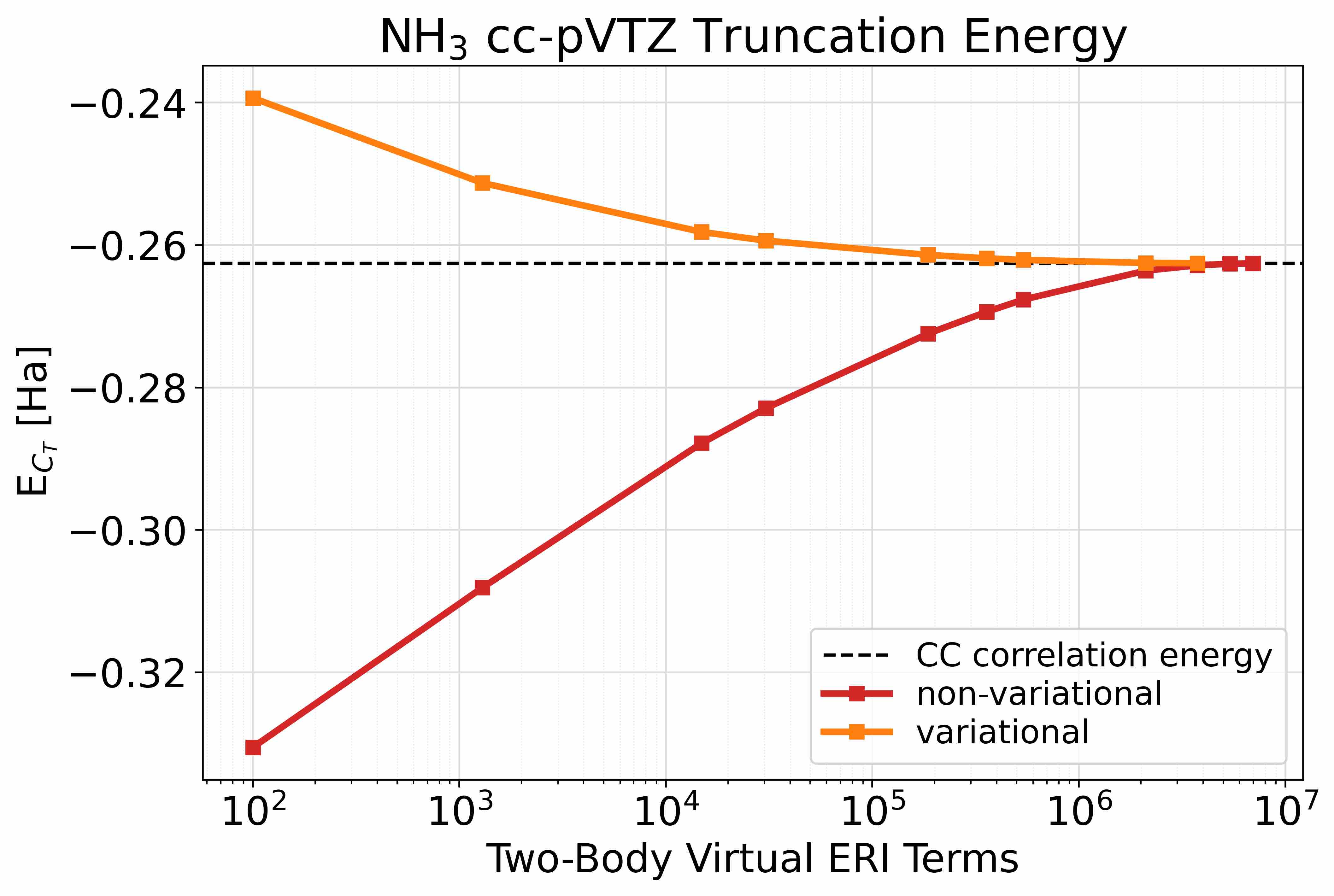
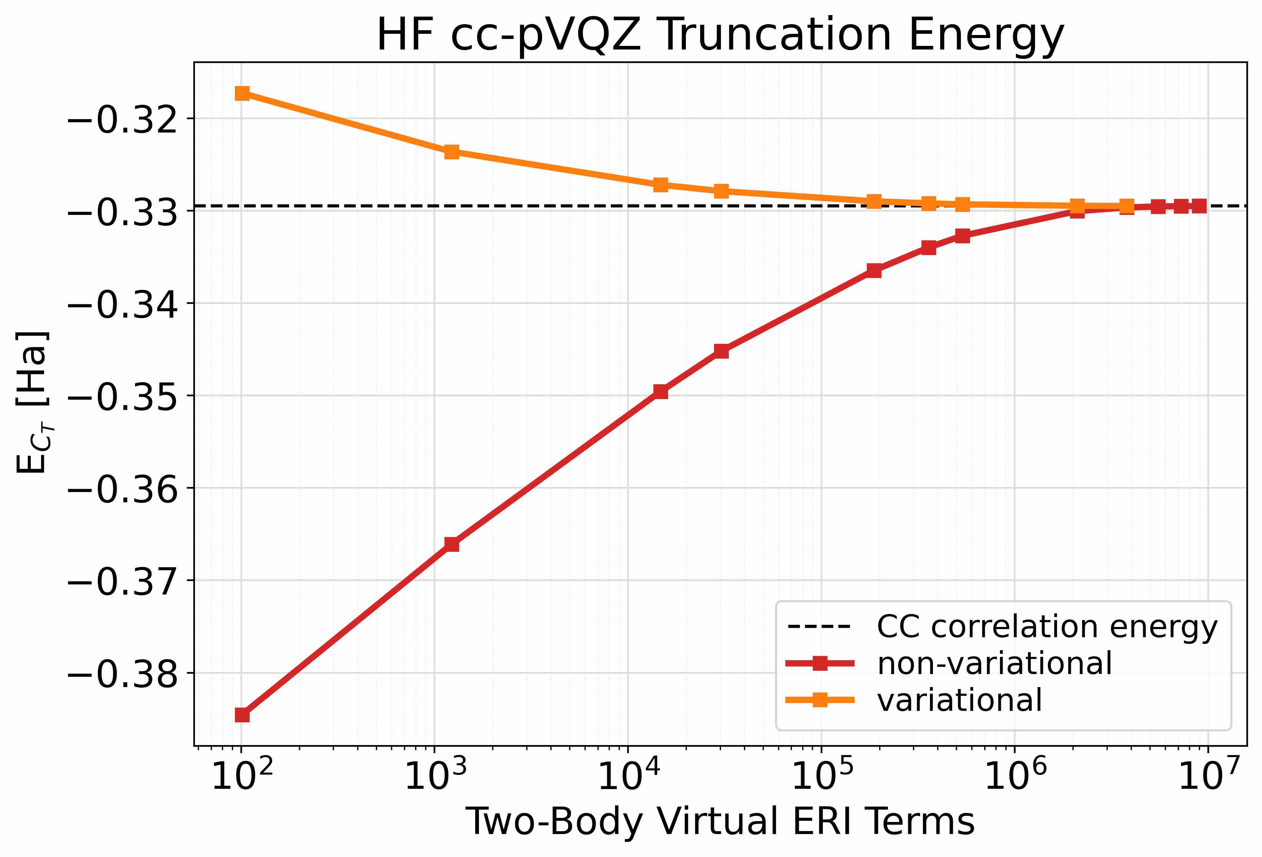
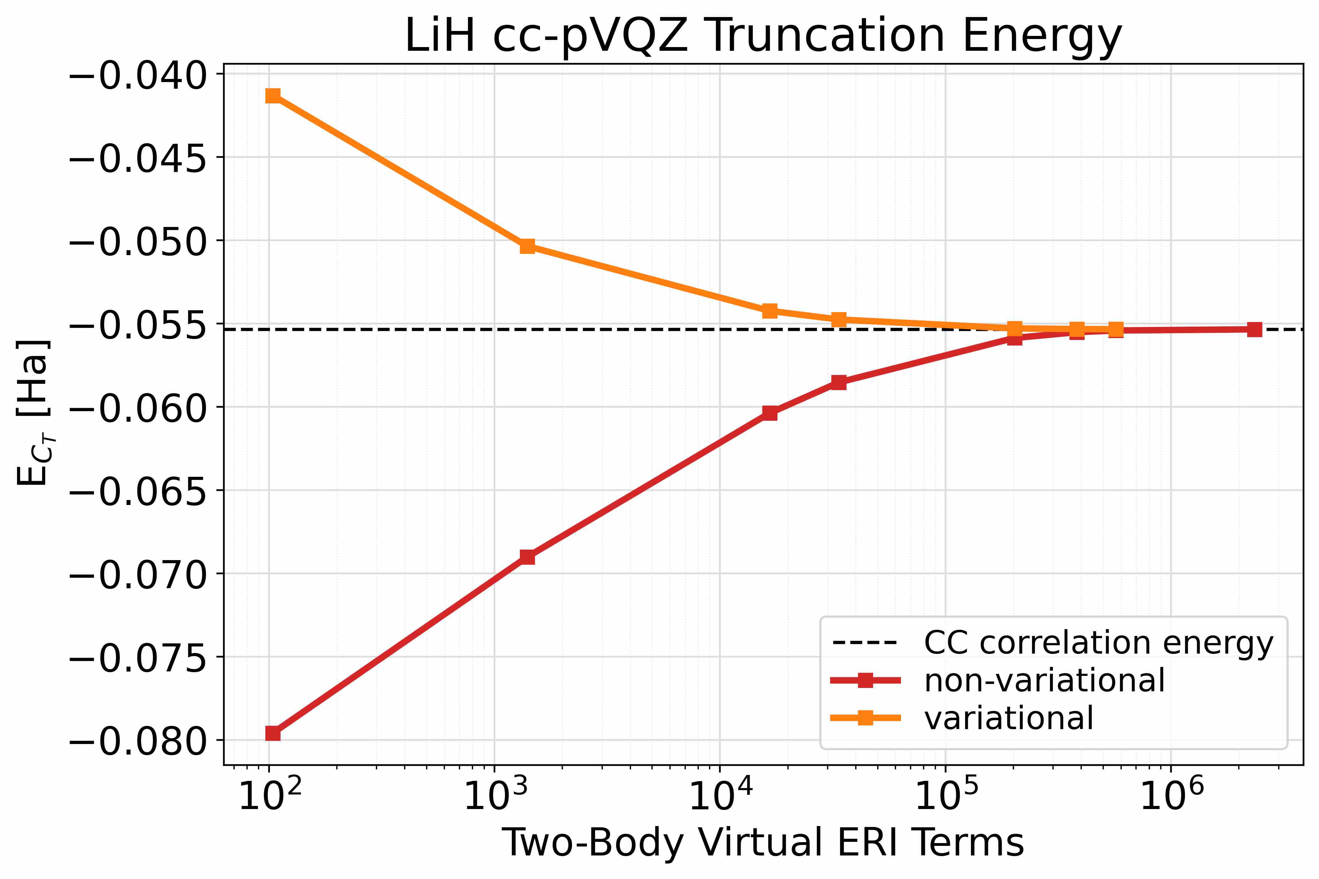
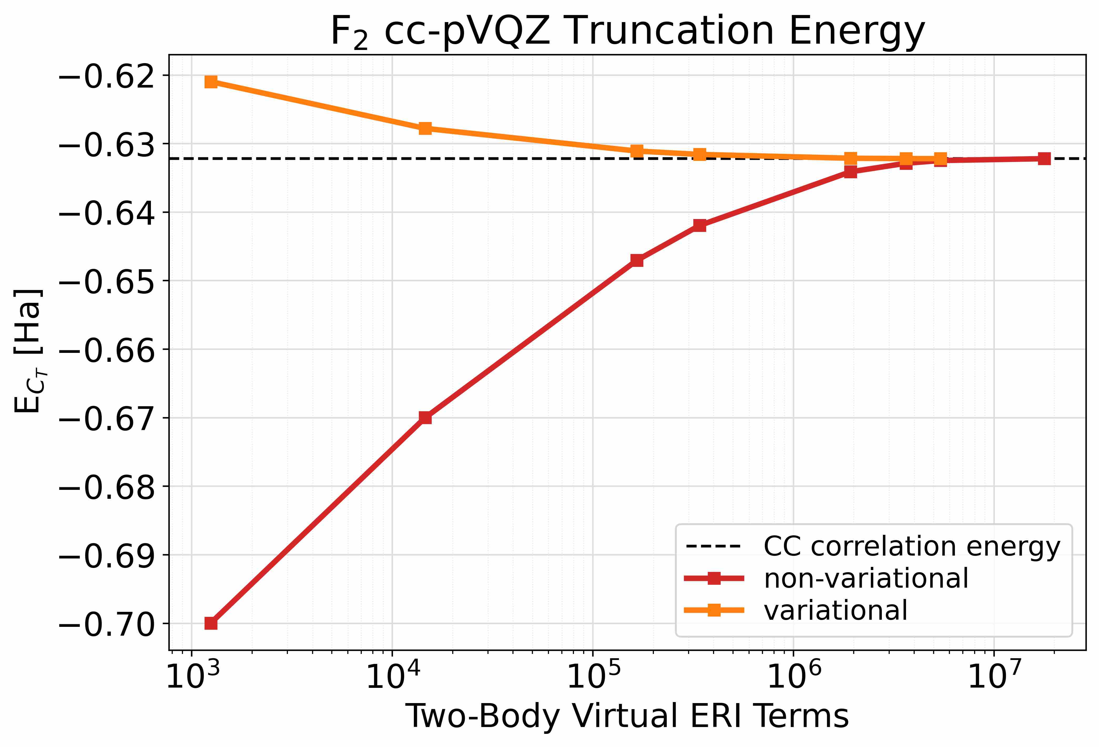
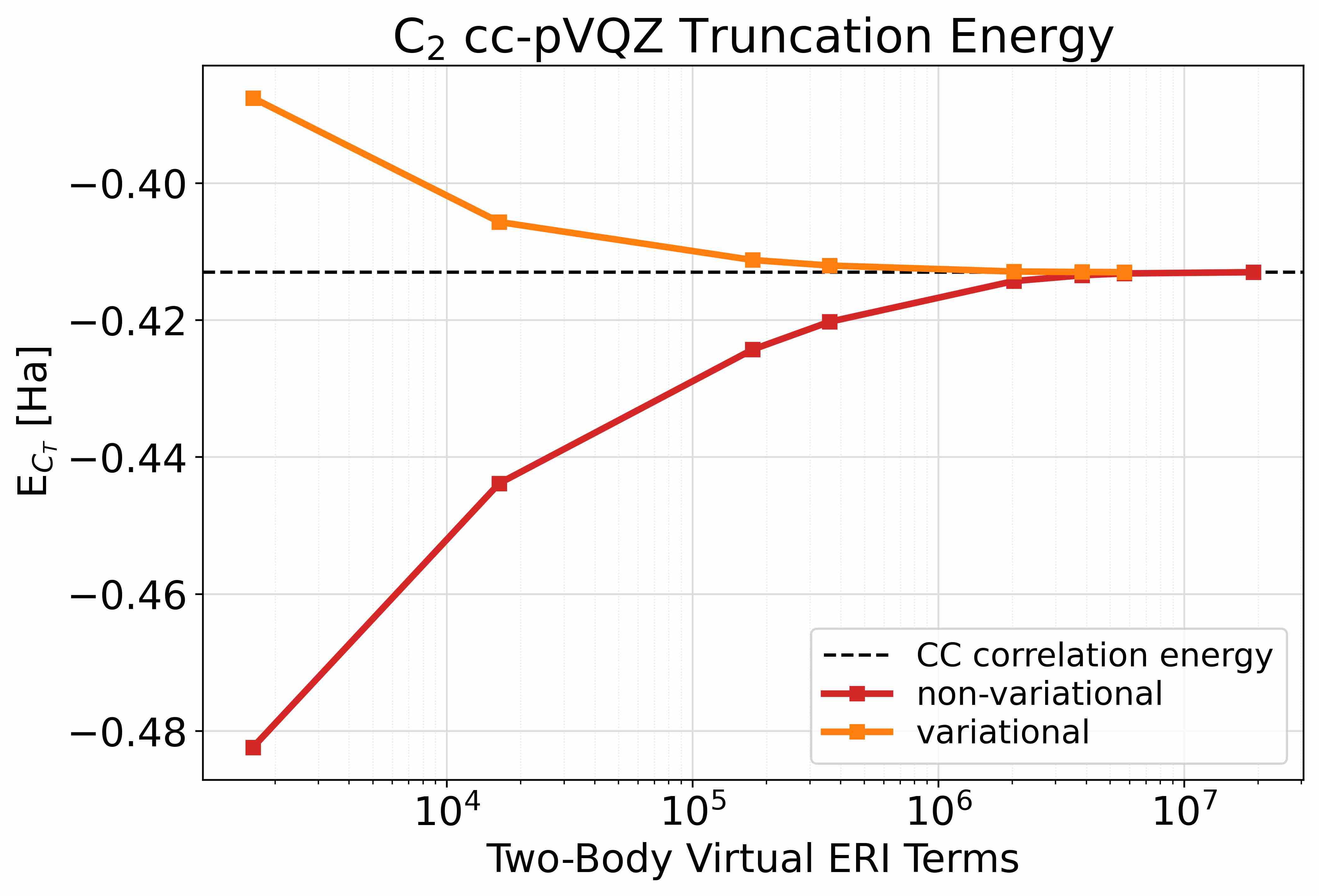
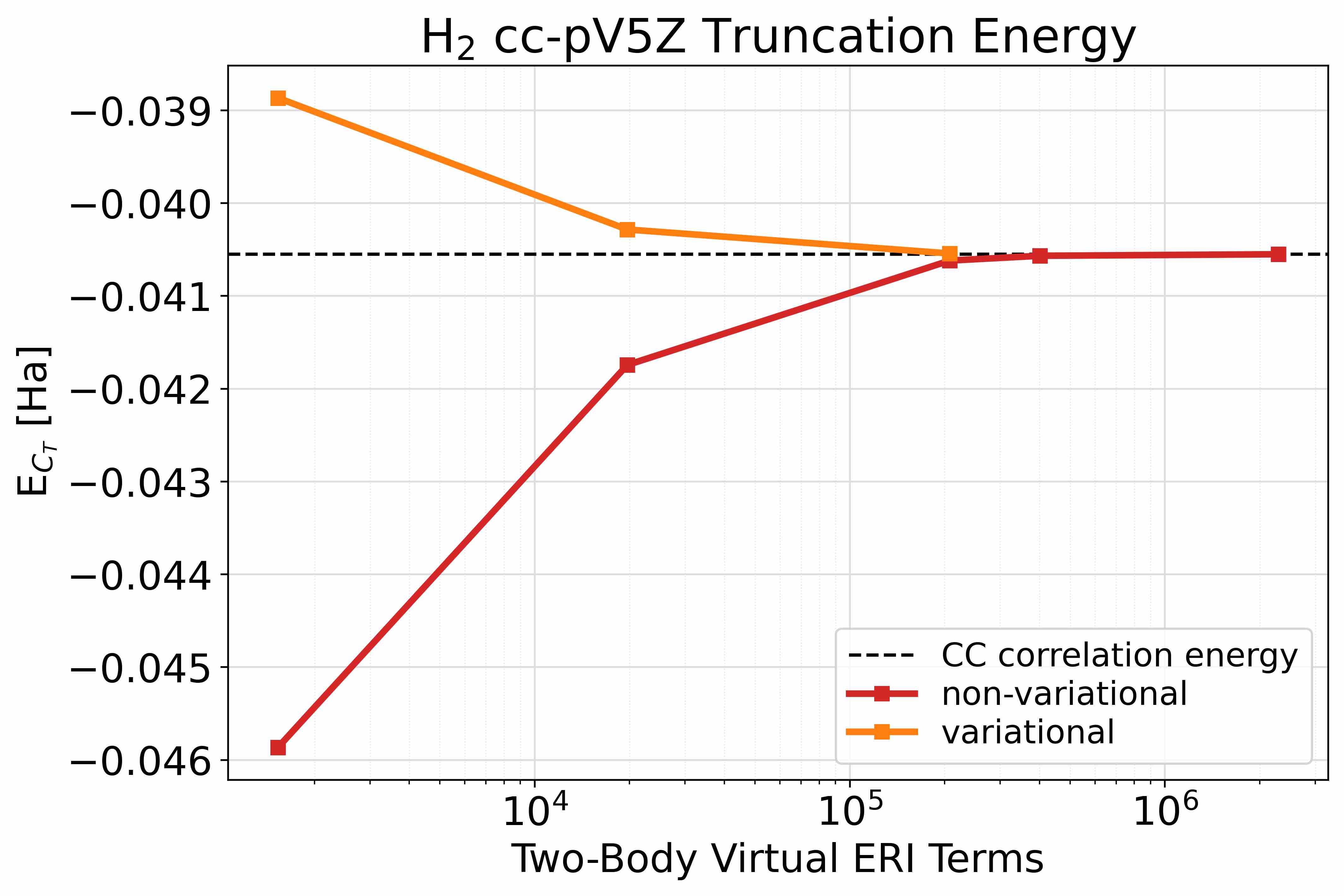
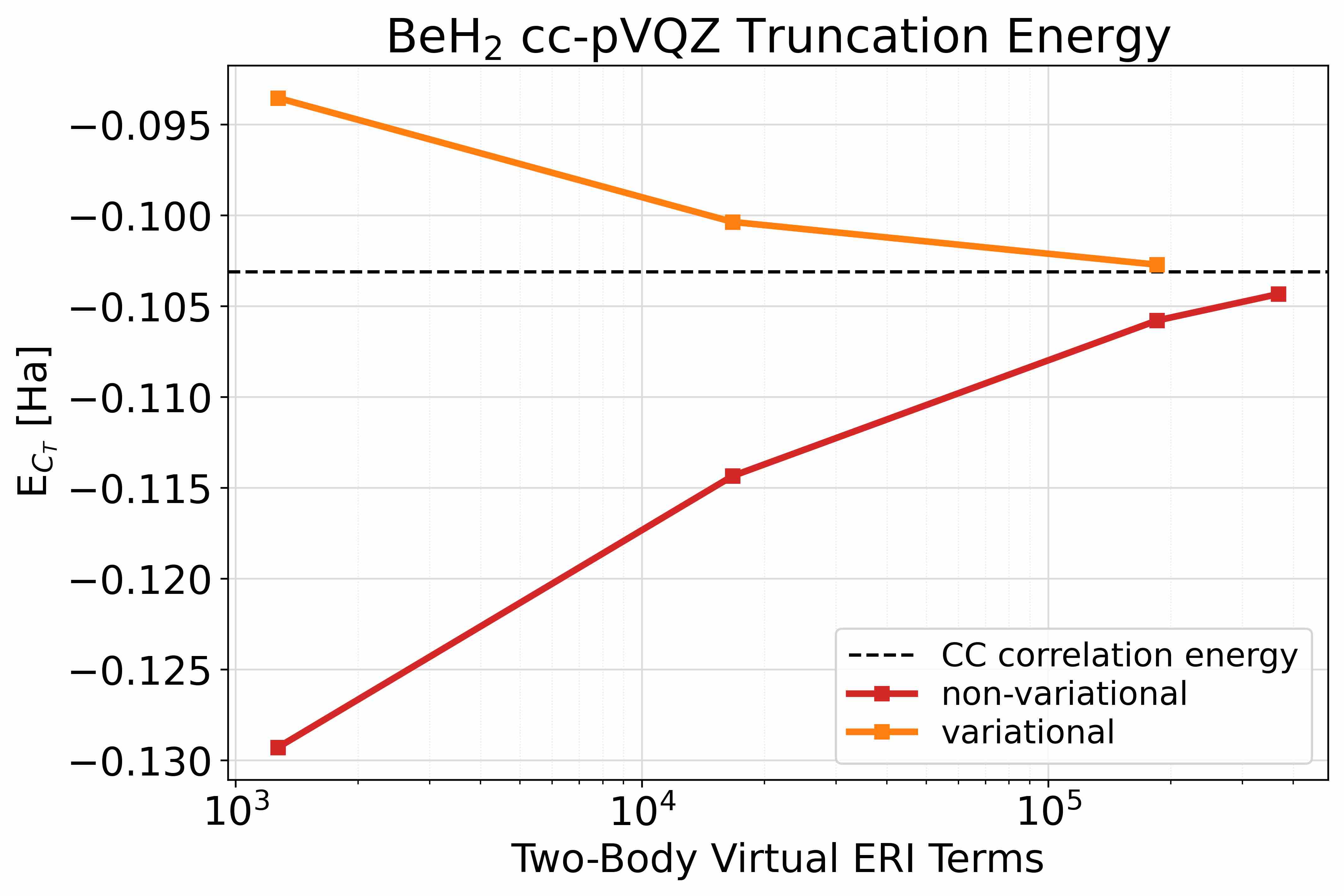
Figure 7: The semi-logarithmic plots of the number of $vvvv$ terms added into the truncated Hamiltonian versus the approximate coupled cluster correlation energy after applying variational and non-variational SQuISH using to the NH3, HF, LiH, F2, C2, H2, and BeH2 Hamiltonians using coupled cluster.

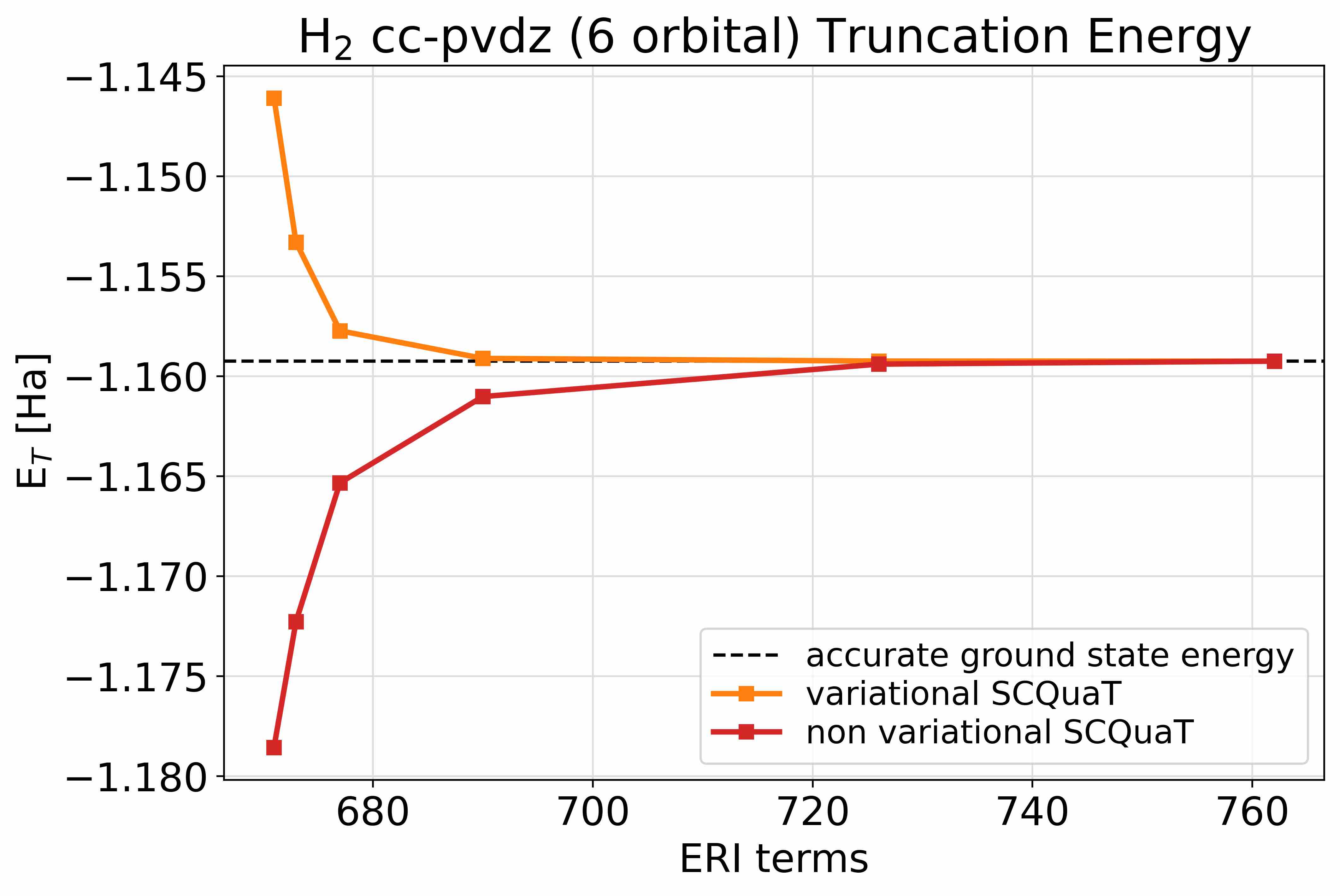
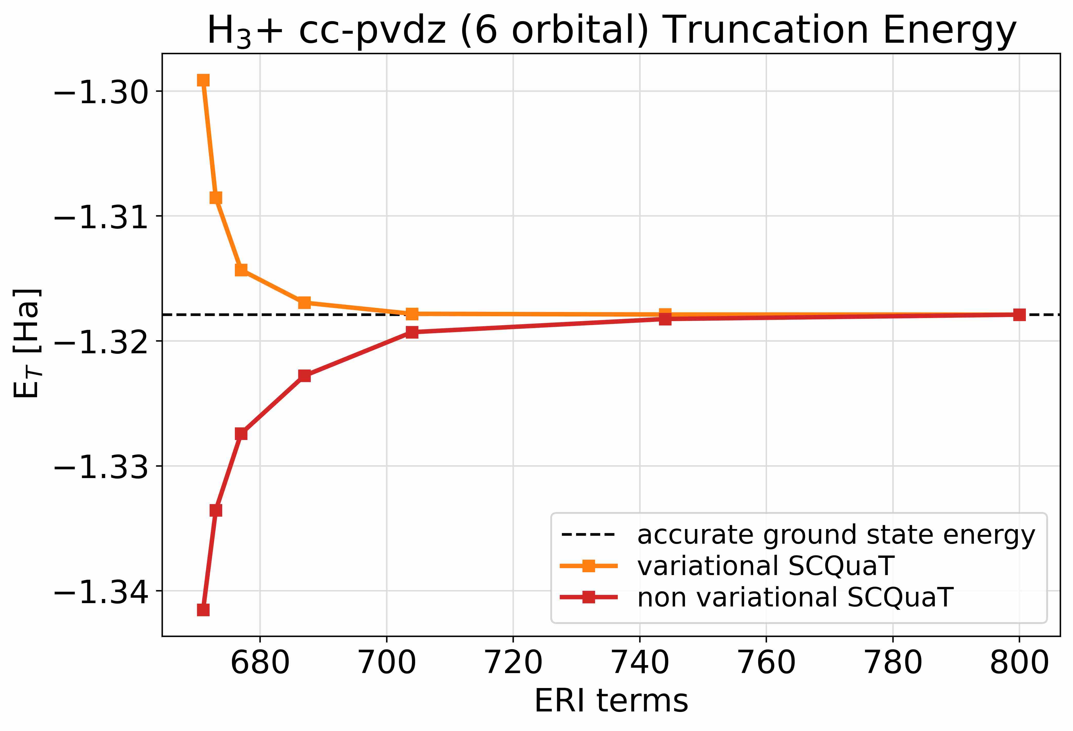
Figure 8: The plots of the number of $vvvv$ terms added into the truncated Hamiltonian versus the approximate energy after applying variational and non-variational SQuISH for the H2 and H3+ Hamiltonians using configuration interaction.

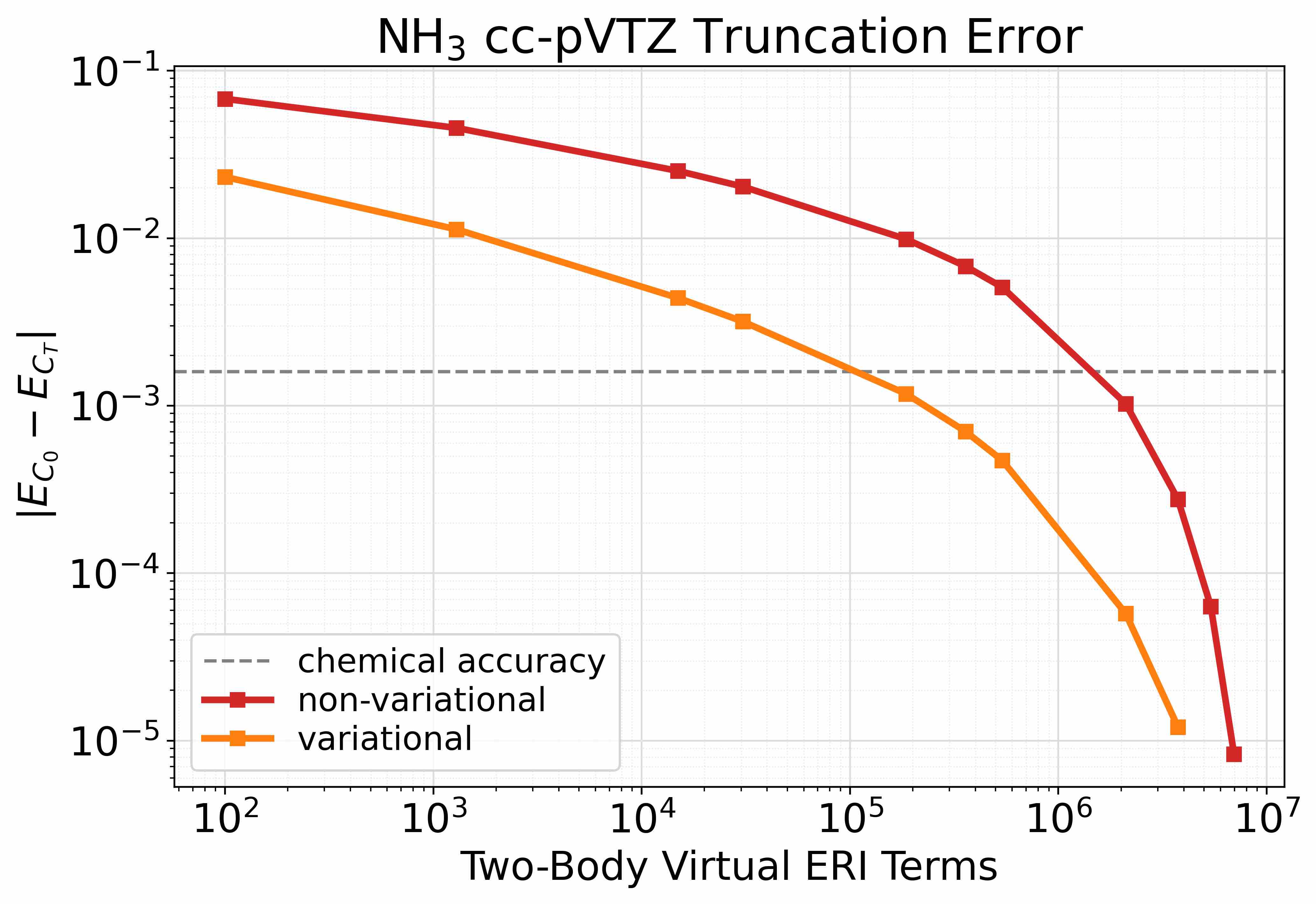
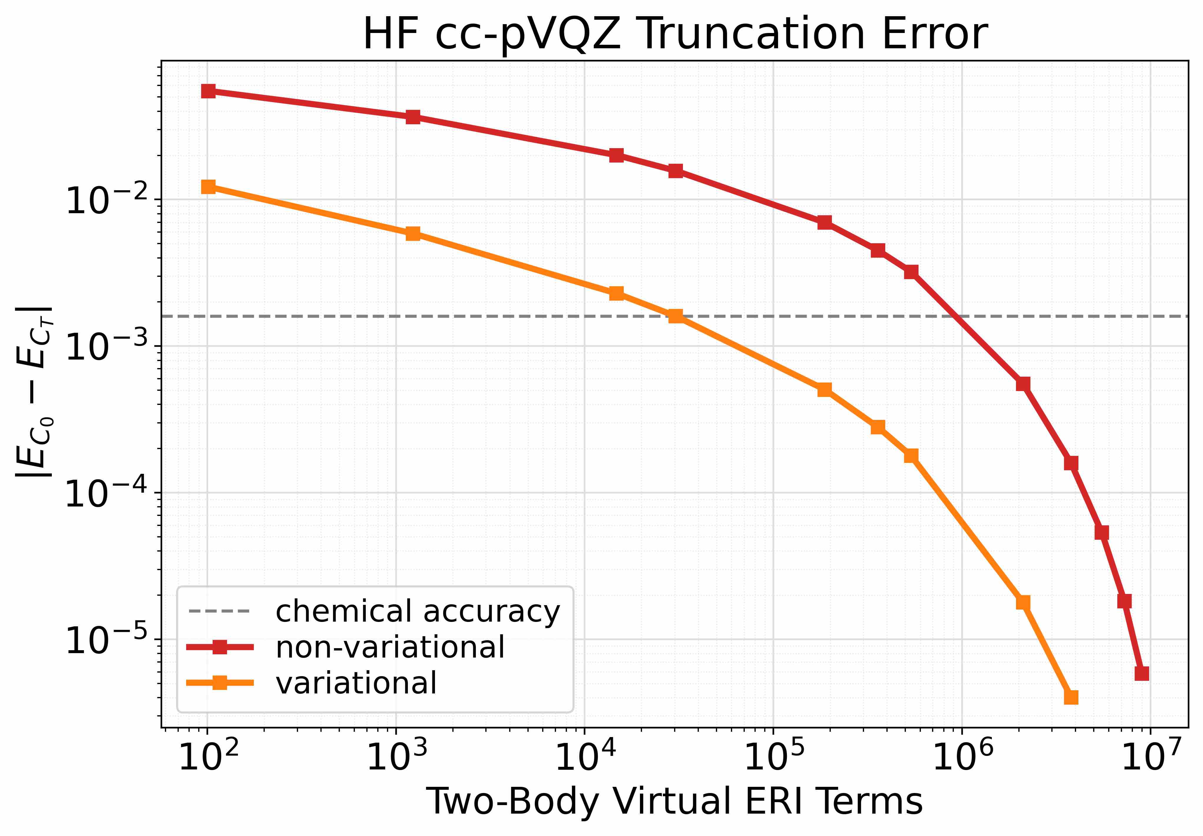
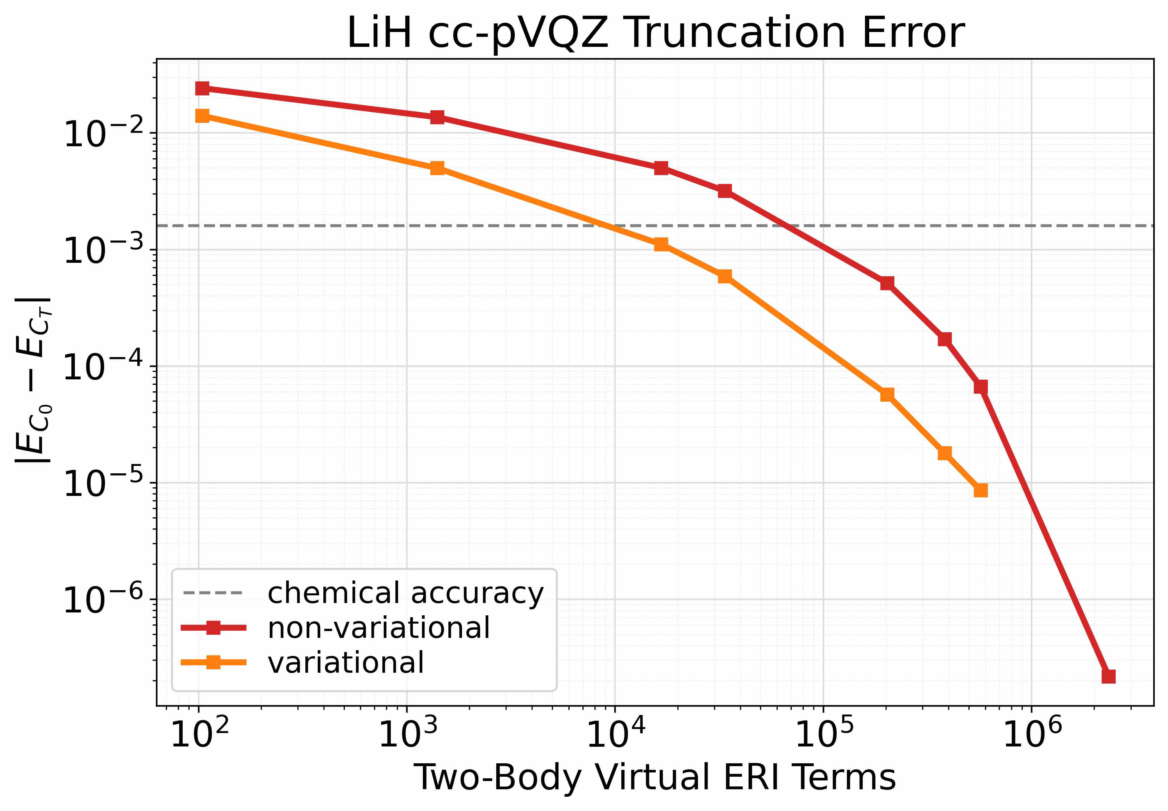
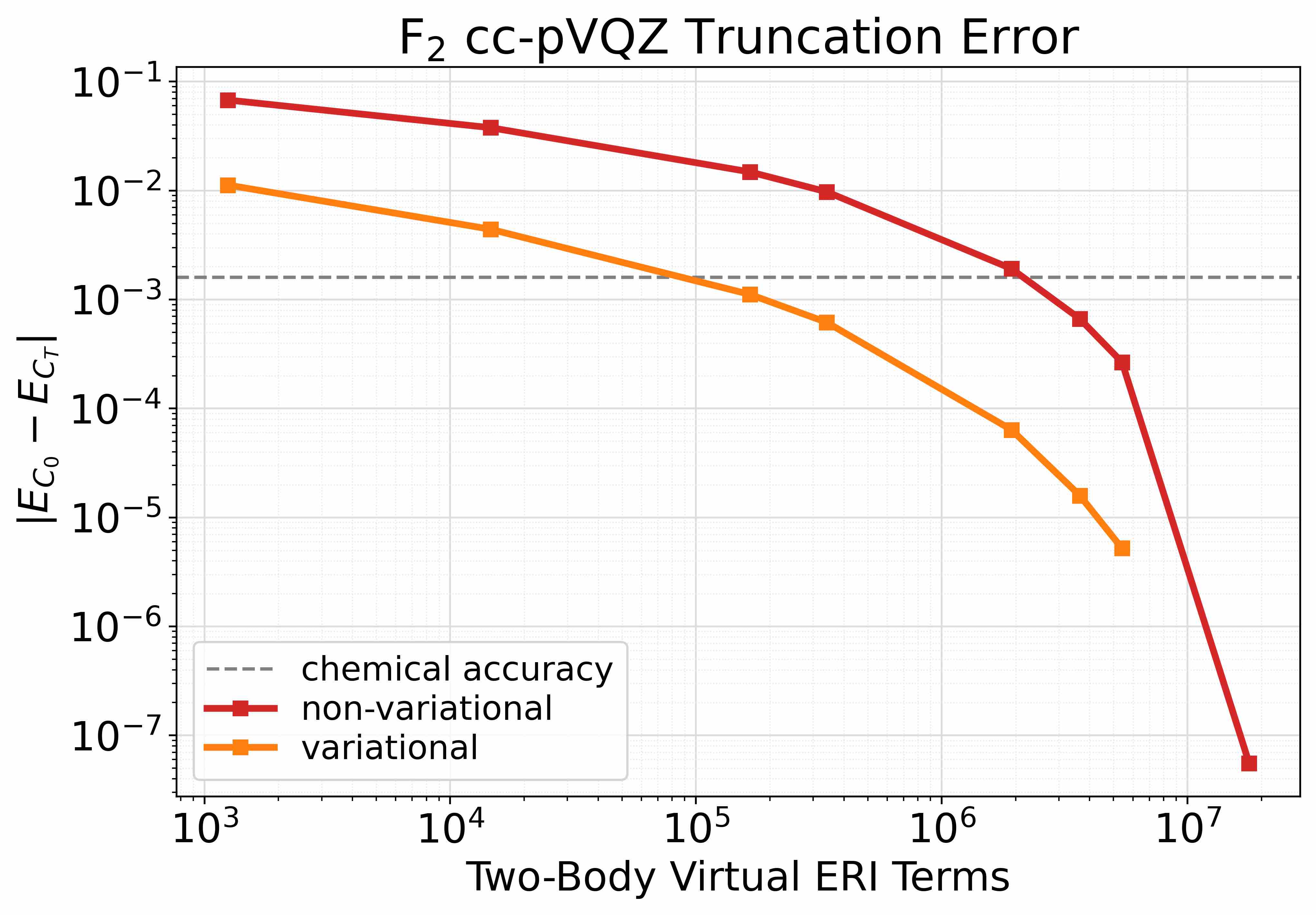
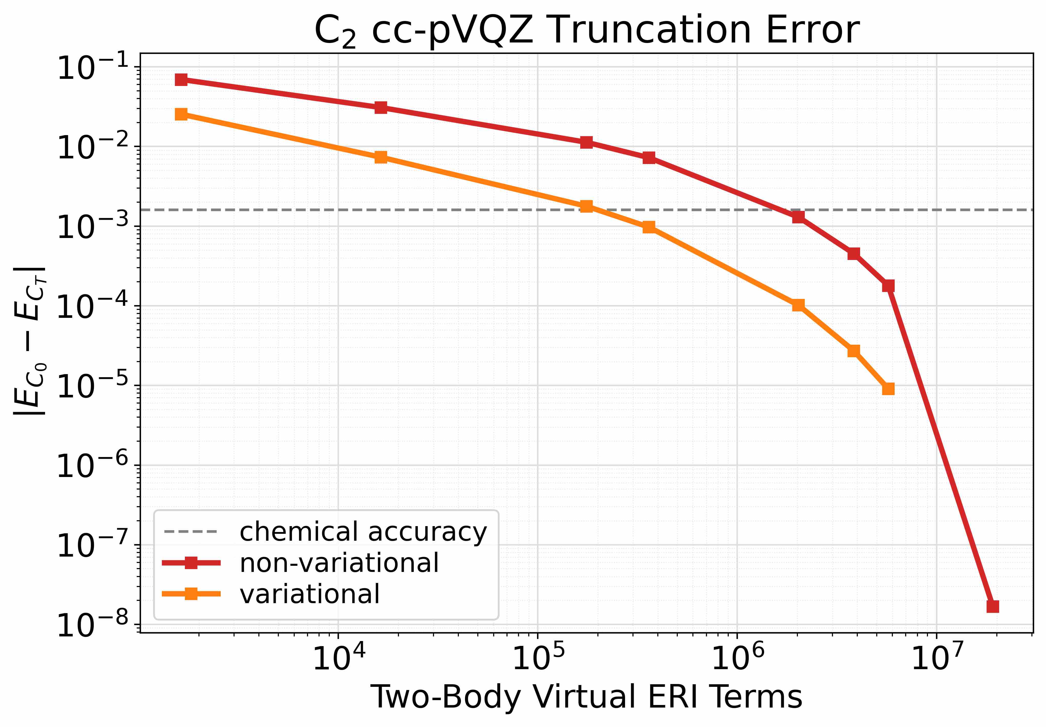
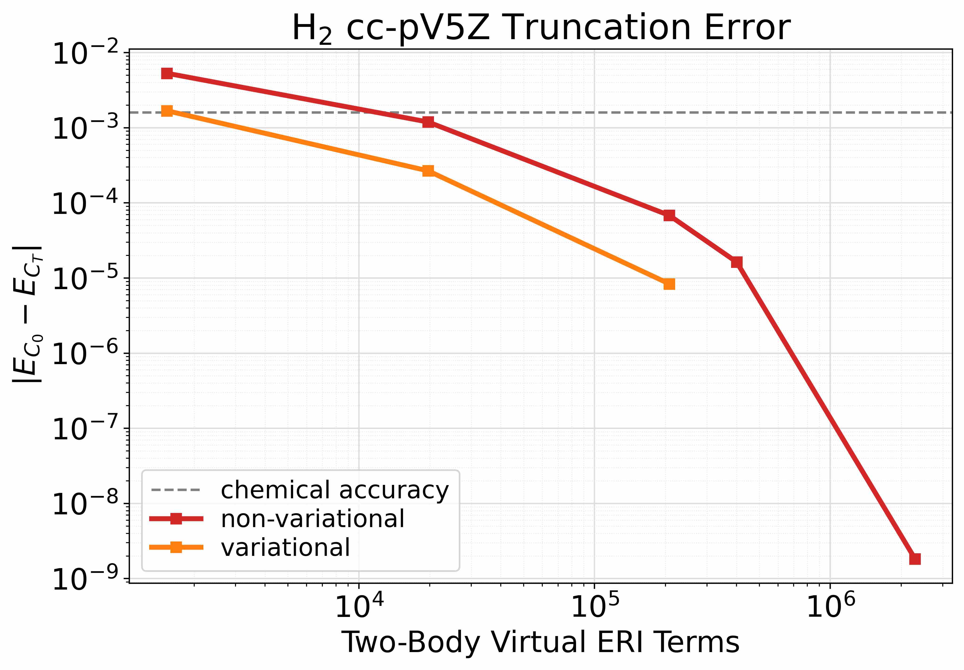
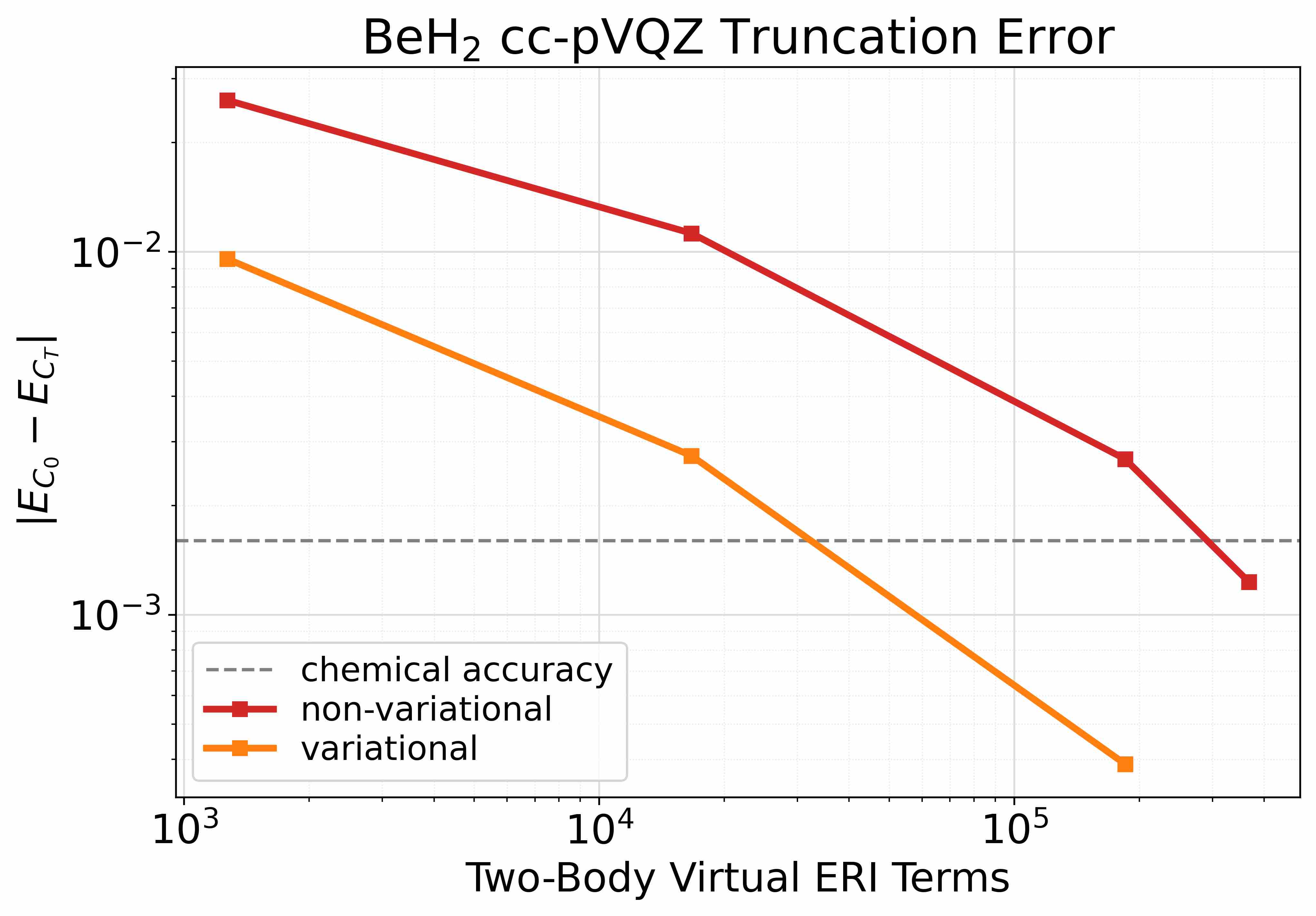
Figure 9: The plots of the number of $vvvv$ terms added into the truncated Hamiltonian versus the absolute value of the error after applying variational and non-variational SQuISH to the NH3, HF, LiH, F2, C2, H2, and BeH2 Hamiltonians using coupled cluster.

Here show the plots for each of the molecules shown in Table 2 and Table 3. Fig. 7 and Fig. 8 are the energy plots for the coupled cluster and configuration interaction runs associated with Table 2 and Table 3, respectively. Fig. 9 and Fig. 10 are the corresponding error plots. We terminated SQuISH once the approximate ground state energy was within $1.5\text{\times}{10}^{-5}$ and $1\text{\times}{10}^{-12}$ of the exact energy for coupled cluster and configuration interaction, respectively.

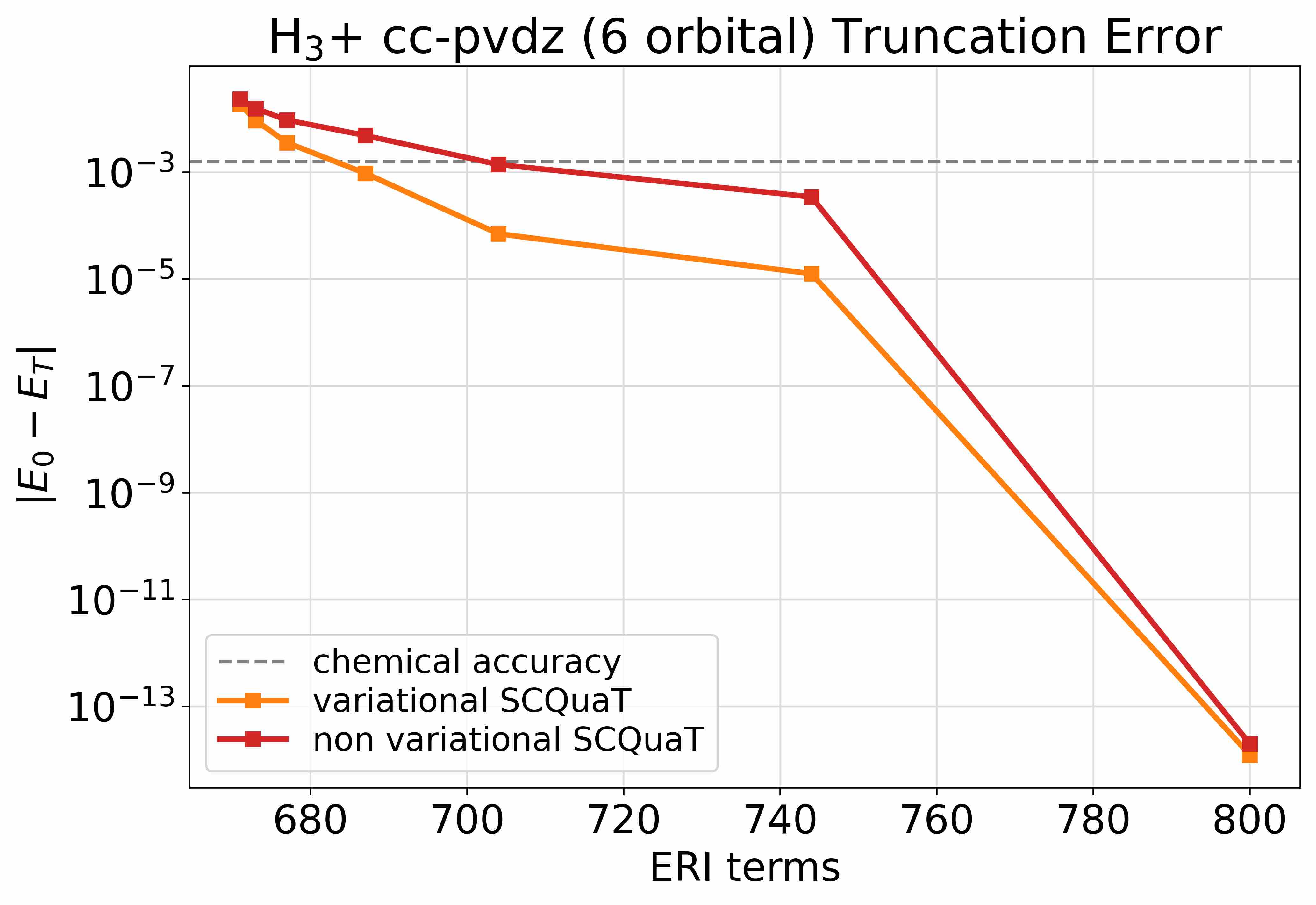
Figure 10: The plots of the number of $vvvv$ terms added into the truncated Hamiltonian versus the absolute value of the error after applying variational and non-variational SQuISH for the H2 and H3+ Hamiltonians using configuration interaction

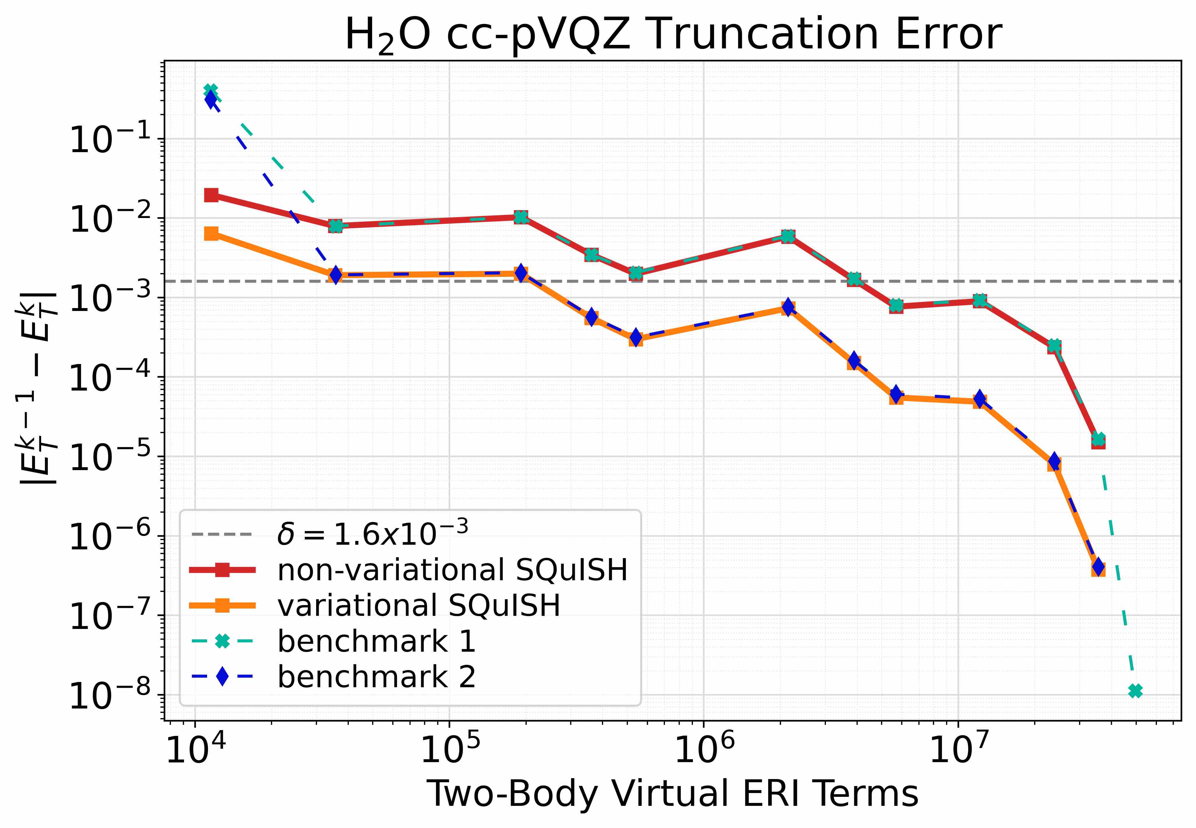
Figure 11: Error plot for the two benchmarks, variational SQuISH, and non-variational SQuISH applied to the H2O ccp-VQZ Hamiltonian using $\absolutevalue{E_{T}^{k-1}-E_{T}^{k}}$.

The results presented in the main paper check for convergence in Step 3 using the exact ground state energy to better understand how well the algorithm performs. This means that SQuISH terminates when $\absolutevalue{E_{0}-E_{T}^{k}}$ is less than the desired accuracy. However, in practice, we are interested in looking at systems to find $E_{0}$ within some error and do not have access to the exact energy. One would employ methods widely used for iterative algorithms. In particular, SQuISH checks for convergence using $\absolutevalue{E_{T}^{k-1}-E_{T}^{k}}<\delta$. Fig. 11 illustrates the results of using $\absolutevalue{E_{T}^{k-1}-E_{T}^{k}}$ to check for accuracy in Step 3 when truncating the H2O cc-pVQZ Hamiltonian using SQuISH. We note that the error is not monotonic.

References

- Helgaker et al. (2012) Trygve Helgaker, Sonia Coriani, Poul Jørgensen, Kasper Kristensen, Jeppe Olsen, and Kenneth Ruud, “Recent advances in wave function-based methods of molecular-property calculations,” Chemical Reviews 112, 543–631 (2012).
- McArdle et al. (2020a) Sam McArdle, Suguru Endo, Alán Aspuru-Guzik, Simon C. Benjamin, and Xiao Yuan, “Quantum computational chemistry,” Rev. Mod. Phys. 92, 015003 (2020a).
- Bauer et al. (2020) Bela Bauer, Sergey Bravyi, Mario Motta, and Garnet Kin-Lic Chan, “Quantum algorithms for quantum chemistry and quantum materials science,” Chemical Reviews 120, 12685–12717 (2020).
- Thøgersen and Olsen (2004) L. Thøgersen and J. Olsen, “A coupled cluster and full configuration interaction study of CN and CN-”,” Chemical Physics Letters 393, 36–43 (2004).
- Alán et al. (2005) Aspuru-Guzik Alán, Anthony D. Dutoi, Peter J. Love, and Martin Head-Gordon, “Simulated quantum computation of molecular energies,” (2005).
- Szabo and Ostlund (2012) Attila Szabo and Neil S Ostlund, Modern quantum chemistry: introduction to advanced electronic structure theory (Courier Corporation, 2012).
- Helgaker et al. (2014) Trygve Helgaker, Poul Jorgensen, and Jeppe Olsen, Molecular electronic-structure theory (John Wiley & Sons, 2014).
- McArdle et al. (2020b) Sam McArdle, Suguru Endo, Alán Aspuru-Guzik, Simon C Benjamin, and Xiao Yuan, “Quantum computational chemistry,” Reviews of Modern Physics 92, 015003 (2020b).
- Kitaev (1995) A. Yu. Kitaev, “Quantum measurements and the abelian stabilizer problem,” (1995).
- Abrams and Lloyd (1999) Daniel S. Abrams and Seth Lloyd, “Quantum algorithm providing exponential speed increase for finding eigenvalues and eigenvectors,” Physical Review Letters 83, 5162–5165 (1999).
- Trotter (1959) Hale F Trotter, “On the product of semi-groups of operators,” Proceedings of the American Mathematical Society 10, 545–551 (1959).
- Suzuki (1976) Masuo Suzuki, “Generalized Trotter’s formula and systematic approximants of exponential operators and inner derivations with applications to many-body problems,” Communications in Mathematical Physics 51, 183–190 (1976).
- Lloyd (1996) Seth Lloyd, “Universal quantum simulators,” Science 273, 1073–1078 (1996).
- Aharonov and Ta-Shma (2003) Dorit Aharonov and Amnon Ta-Shma, “Adiabatic quantum state generation and statistical zero knowledge,” in Proceedings of the thirty-fifth annual ACM symposium on Theory of computing (2003) pp. 20–29.
- Berry et al. (2007) Dominic W Berry, Graeme Ahokas, Richard Cleve, and Barry C Sanders, “Efficient quantum algorithms for simulating sparse hamiltonians,” Communications in Mathematical Physics 270, 359–371 (2007).
- Hadfield and Papageorgiou (2018) Stuart Hadfield and Anargyros Papageorgiou, “Divide and conquer approach to quantum Hamiltonian simulation,” New Journal of Physics 20, 043003 (2018).
- Childs et al. (2021a) Andrew M Childs, Yuan Su, Minh C Tran, Nathan Wiebe, and Shuchen Zhu, “Theory of Trotter error with commutator scaling,” Physical Review X 11, 011020 (2021a).
- Zhang (2012) Chi Zhang, “Randomized algorithms for hamiltonian simulation,” in Monte Carlo and Quasi-Monte Carlo Methods 2010 (Springer, 2012) pp. 709–719.
- Campbell (2019) Earl Campbell, “Random compiler for fast hamiltonian simulation,” Physical Review Letters 123 (2019), 10.1103/physrevlett.123.070503.
- Childs et al. (2019) Andrew M Childs, Aaron Ostrander, and Yuan Su, “Faster quantum simulation by randomization,” Quantum 3, 182 (2019).
- Low and Chuang (2017) Guang Hao Low and Isaac L Chuang, “Optimal hamiltonian simulation by quantum signal processing,” Physical review letters 118, 010501 (2017).
- Low and Chuang (2019) Guang Hao Low and Isaac L. Chuang, “Hamiltonian simulation by qubitization,” Quantum 3, 163 (2019).
- Seeley et al. (2012a) Jacob T. Seeley, Martin J. Richard, and Peter J. Love, “The Bravyi-Kitaev transformation for quantum computation of electronic structure,” AIP Publishing (2012a).
- Hastings et al. (2015) Matthew B. Hastings, Dave Wecker, Bela Bauer, and Matthias Troyer, “Improving quantum algorithms for quantum chemistry,” Quantum Info. Comput. 15 (2015).
- Childs et al. (2021b) Andrew M. Childs, Yuan Su, Minh C. Tran, Nathan Wiebe, and Shuchen Zhu, “Theory of trotter error with commutator scaling,” Physical Review X 11 (2021b), 10.1103/physrevx.11.011020.
- Loaiza et al. (2022) Ignacio Loaiza, Alireza Marefat Khah, Nathan Wiebe, and Artur F. Izmaylov, “Reducing molecular electronic hamiltonian simulation cost for linear combination of unitaries approaches,” (2022).
- Zurek (1981) W. H. Zurek, “Pointer basis of quantum apparatus: Into what mixture does the wave packet collapse?” Phys. Rev. D 24, 1516–1525 (1981).
- Joos and Zeh (1985) E. Joos and H. D. Zeh, “The emergence of classical properties through interaction with the environment,” Zeitschrift für Physik B Condensed Matter 59, 223–243 (1985).
- Preskill (2012) John Preskill, “Quantum computing and the entanglement frontier,” (2012).
- Preskill (2018) John Preskill, “Quantum computing in the NISQ era and beyond,” Quantum 2, 79 (2018).
- Wecker et al. (2014) Dave Wecker, Bela Bauer, Bryan K Clark, Matthew B Hastings, and Matthias Troyer, “Gate-count estimates for performing quantum chemistry on small quantum computers,” Physical Review A 90, 022305 (2014).
- McClean et al. (2014) Jarrod R McClean, Ryan Babbush, Peter J Love, and Alán Aspuru-Guzik, “Exploiting locality in quantum computation for quantum chemistry,” The journal of physical chemistry letters 5, 4368–4380 (2014).
- Poulin et al. (2015) David Poulin, Matthew B Hastings, Dave Wecker, Nathan Wiebe, Andrew C Doherty, and Matthias Troyer, “The Trotter step size required for accurate quantum simulation of quantum chemistry,” Quantum Inf. Comput. 15, 361–84 (2015).
- Babbush et al. (2015) Ryan Babbush, Jarrod McClean, Dave Wecker, Alán Aspuru-Guzik, and Nathan Wiebe, “Chemical basis of Trotter-Suzuki errors in quantum chemistry simulation,” Physical Review A 91, 022311 (2015).
- Babbush et al. (2018a) Ryan Babbush, Nathan Wiebe, Jarrod McClean, James McClain, Hartmut Neven, and Garnet Kin-Lic Chan, “Low-depth quantum simulation of materials,” Phys. Rev. X 8, 011044 (2018a).
- Babbush et al. (2018b) Ryan Babbush, Craig Gidney, Dominic W. Berry, Nathan Wiebe, Jarrod McClean, Alexandru Paler, Austin Fowler, and Hartmut Neven, “Encoding electronic spectra in quantum circuits with linear t complexity,” Phys. Rev. X 8, 041015 (2018b).
- Low and Wiebe (2019) Guang Hao Low and Nathan Wiebe, “Hamiltonian simulation in the interaction picture,” arXiv.org (2019).
- Kivlichan et al. (2020) Ian D. Kivlichan, Craig Gidney, Dominic W. Berry, Nathan Wiebe, Jarrod McClean, Wei Sun, Zhang Jiang, Nicholas Rubin, Austin Fowler, Alán Aspuru-Guzik, and et al., “Improved fault-tolerant quantum simulation of condensed-phase correlated electrons via Trotterization,” Quantum (2020).
- McClean et al. (2021) JR McClean, FM Faulstich, Q Zhu, B O’Gorman, Y Qiu, SR White, R Babbush, and L Lin, “Discontinuous Galerkin discretization for quantum simulation of chemistry,” New Journal of Physics (2021).
- Lee et al. (2021) Joonho Lee, Dominic W. Berry, Craig Gidney, William J. Huggins, Jarrod R. McClean, Nathan Wiebe, and Ryan Babbush, “Even more efficient quantum computations of chemistry through tensor hypercontraction,” PRX Quantum 2, 030305 (2021).
- Motta et al. (2021) Mario Motta, Erika Ye, Jarrod R McClean, Zhendong Li, Austin J Minnich, Ryan Babbush, and Garnet Kin Chan, “Low rank representations for quantum simulation of electronic structure,” npj Quantum Information 7, 1–7 (2021).
- Tubman et al. (2016) Norm M. Tubman, Joonho Lee, Tyler Y. Takeshita, Martin Head-Gordon, and K. Birgitta Whaley, “A deterministic alternative to the full configuration interaction quantum monte carlo method,” AIP Publishing (2016).
- Tubman et al. (2018) Norm M. Tubman, Daniel S. Levine, Diptarka Hait, Martin Head-Gordon, and K. Birgitta Whaley, “An efficient deterministic perturbation theory for selected configuration interaction methods,” (2018).
- Tubman et al. (2020) Norm M Tubman, C Daniel Freeman, Daniel S Levine, Diptarka Hait, Martin Head-Gordon, and K Birgitta Whaley, “Modern approaches to exact diagonalization and selected configuration interaction with the adaptive sampling CI method,” Journal of chemical theory and computation 16, 2139—2159 (2020).
- Whitfield et al. (2011) James D Whitfield, Jacob Biamonte, and Alán Aspuru-Guzik, “Simulation of electronic structure hamiltonians using quantum computers,” Molecular Physics 109, 735–750 (2011).
- Seeley et al. (2012b) Jacob T Seeley, Martin J Richard, and Peter J Love, “The bravyi-kitaev transformation for quantum computation of electronic structure,” The Journal of chemical physics 137, 224109 (2012b).
- Setia et al. (2019) Kanav Setia, Sergey Bravyi, Antonio Mezzacapo, and James D Whitfield, “Superfast encodings for fermionic quantum simulation,” Physical Review Research 1, 033033 (2019).
- Peruzzo et al. (2014) Alberto Peruzzo, Jarrod McClean, Peter Shadbolt, Man-Hong Yung, Xiao-Qi Zhou, Peter J Love, Alán Aspuru-Guzik, and Jeremy L O’brien, “A variational eigenvalue solver on a photonic quantum processor,” Nature communications 5, 1–7 (2014).
- McClean et al. (2016) Jarrod R McClean, Jonathan Romero, Ryan Babbush, and Alán Aspuru-Guzik, “The theory of variational hybrid quantum-classical algorithms,” New Journal of Physics 18, 023023 (2016).
- Cerezo et al. (2021) Marco Cerezo, Andrew Arrasmith, Ryan Babbush, Simon C Benjamin, Suguru Endo, Keisuke Fujii, Jarrod R McClean, Kosuke Mitarai, Xiao Yuan, Lukasz Cincio, et al., “Variational quantum algorithms,” Nature Reviews Physics 3, 625–644 (2021).
- Tilly et al. (2021) Jules Tilly, Hongxiang Chen, Shuxiang Cao, Dario Picozzi, Kanav Setia, Ying Li, Edward Grant, Leonard Wossnig, Ivan Rungger, George H Booth, et al., “The variational quantum eigensolver: a review of methods and best practices,” arXiv preprint arXiv:2111.05176 (2021).
- Bharti et al. (2022) Kishor Bharti, Alba Cervera-Lierta, Thi Ha Kyaw, Tobias Haug, Sumner Alperin-Lea, Abhinav Anand, Matthias Degroote, Hermanni Heimonen, Jakob S Kottmann, Tim Menke, et al., “Noisy intermediate-scale quantum algorithms,” Reviews of Modern Physics 94, 015004 (2022).
- Huembeli and Dauphin (2021) Patrick Huembeli and Alexandre Dauphin, “Characterizing the loss landscape of variational quantum circuits,” Quantum Science and Technology 6, 025011 (2021).
- Bittel and Kliesch (2021) Lennart Bittel and Martin Kliesch, “Training variational quantum algorithms is NP-hard,” Physical Review Letters 127, 120502 (2021).
- McClean et al. (2018) Jarrod R McClean, Sergio Boixo, Vadim N Smelyanskiy, Ryan Babbush, and Hartmut Neven, “Barren plateaus in quantum neural network training landscapes,” Nature communications 9, 1–6 (2018).
- Wang et al. (2021) Samson Wang, Enrico Fontana, Marco Cerezo, Kunal Sharma, Akira Sone, Lukasz Cincio, and Patrick J Coles, “Noise-induced barren plateaus in variational quantum algorithms,” Nature communications 12, 1–11 (2021).
- Izmaylov et al. (2019) Artur F Izmaylov, Tzu-Ching Yen, and Ilya G Ryabinkin, “Revising the measurement process in the variational quantum eigensolver: is it possible to reduce the number of separately measured operators?” Chemical science 10, 3746–3755 (2019).
- Huggins et al. (2021) William J Huggins, Jarrod R McClean, Nicholas C Rubin, Zhang Jiang, Nathan Wiebe, K Birgitta Whaley, and Ryan Babbush, “Efficient and noise resilient measurements for quantum chemistry on near-term quantum computers,” npj Quantum Information 7, 1–9 (2021).
- Mohammadbagherpoor et al. (2019a) Hamed Mohammadbagherpoor, Young-Hyun Oh, Anand Singh, Xianqing Yu, and Andy J. Rindos, “Experimental challenges of implementing quantum phase estimation algorithms on ibm quantum computer,” (2019a).
- Mohammadbagherpoor et al. (2019b) Hamed Mohammadbagherpoor, Young-Hyun Oh, Patrick Dreher, Anand Singh, Xianqing Yu, and Andy J. Rindos, “An improved implementation approach for quantum phase estimation on quantum computers,” in 2019 IEEE International Conference on Rebooting Computing (ICRC) (2019) pp. 1–9.
- et al. (2020) Frank Arute et al., “Hartree-fock on a superconducting qubit quantum computer,” Science 369, 1084–1089 (2020).
- Huang et al. (2020) Hsin-Yuan Huang, Richard Kueng, and John Preskill, “Predicting many properties of a quantum system from very few measurements,” Nature Physics 16, 1050–1057 (2020).
- Elben et al. (2022) Andreas Elben, Steven T. Flammia, Hsin-Yuan Huang, Richard Kueng, John Preskill, Benoît Vermersch, and Peter Zoller, “The randomized measurement toolbox,” (2022).
- Zhao et al. (2021) Andrew Zhao, Nicholas C. Rubin, and Akimasa Miyake, “Fermionic partial tomography via classical shadows,” Physical Review Letters 127 (2021), 10.1103/physrevlett.127.110504.
- Wan et al. (2022) Kianna Wan, William J. Huggins, Joonho Lee, and Ryan Babbush, “Matchgate shadows for fermionic quantum simulation,” (2022).
- O’Gorman (2022) Bryan O’Gorman, “Fermionic tomography and learning,” (2022).
- Low (2022) Guang Hao Low, “Classical shadows of fermions with particle number symmetry,” (2022).
- Jiang et al. (2018) Zhang Jiang, Kevin J Sung, Kostyantyn Kechedzhi, Vadim N Smelyanskiy, and Sergio Boixo, “Quantum algorithms to simulate many-body physics of correlated fermions,” Physical Review Applied 9, 044036 (2018).
- Bartlett et al. (1989) Rodney J. Bartlett, Stanislaw A. Kucharski, and Jozef Noga, “Alternative coupled-cluster ansätze ii. the unitary coupled-cluster method,” Chemical Physics Letters 155, 133–140 (1989).
- Hoffmann and Simons (1988) Mark R. Hoffmann and Jack Simons, “A unitary multiconfigurational coupled‐cluster method: Theory and applications,” Journal of Chemical Physics 88, 993–1002 (1988).
- Wecker et al. (2015) Dave Wecker, Matthew B. Hastings, and Matthias Troyer, “Progress towards practical quantum variational algorithms,” Physical Review A 92 (2015), 10.1103/physreva.92.042303.
- Kandala et al. (2017) Abhinav Kandala, Antonio Mezzacapo, Kristan Temme, Maika Takita, Markus Brink, Jerry M. Chow, and Jay M. Gambetta, “Hardware-efficient variational quantum eigensolver for small molecules and quantum magnets,” Nature 549, 242–246 (2017).
- Feller et al. (2008) David Feller, Kirk A. Peterson, and David A. Dixon, “A survey of factors contributing to accurate theoretical predictions of atomization energies and molecular structures.” The Journal of Chemical Physics 129 20, 204105 (2008).
- Johnson (1999) Russell Johnson, “NIST 101. Computational chemistry comparison and benchmark database,” (1999).
- Crosson and Lidar (2021) E. J. Crosson and D. A. Lidar, “Prospects for quantum enhancement with diabatic quantum annealing,” Nature Reviews Physics 3, 466–489 (2021).
- Hauke et al. (2020) Philipp Hauke, Helmut G Katzgraber, Wolfgang Lechner, Hidetoshi Nishimori, and William D Oliver, “Perspectives of quantum annealing: methods and implementations,” Reports on Progress in Physics 83, 054401 (2020).
- Brady et al. (2021) Lucas T. Brady, Christopher L. Baldwin, Aniruddha Bapat, Yaroslav Kharkov, and Alexey V. Gorshkov, “Optimal protocols in quantum annealing and quantum approximate optimization algorithm problems,” Phys. Rev. Lett. 126, 070505 (2021).
- Kremenetski et al. (2021a) Vladimir Kremenetski, Carlos Mejuto-Zaera, Stephen J. Cotton, and Norm M. Tubman, “Simulation of adiabatic quantum computing for molecular ground states,” The Journal of Chemical Physics 155, 234106 (2021a).
- Kremenetski et al. (2021b) Vladimir Kremenetski, Tad Hogg, Stuart Hadfield, Stephen J. Cotton, and Norm M. Tubman, “Quantum alternating operator ansatz (QAOA) phase diagrams and applications for quantum chemistry,” (2021b).
- Crawford (2021) Daniel Crawford, “Pycc,” https://github.com/lothian/pycc (2021).
- et al. (2021) MD SAJID ANIS et al., “Qiskit: An open-source framework for quantum computing,” (2021).
- Booth et al. (2009) George H. Booth, Alex J. W. Thom, and Ali Alavi, “Fermion monte carlo without fixed nodes: A game of life, death, and annihilation in slater determinant space.” The Journal of chemical physics 131 5, 054106 (2009).