MUSE-ALMA Haloes VII: Survey Science Goals & Design, Data Processing and Final Catalogues

Abstract

The gas cycling in the circumgalactic regions of galaxies is known to be multi-phase. The MUSE-ALMA Haloes survey gathers a large multi-wavelength observational sample of absorption and emission data with the goal to significantly advance our understanding of the physical properties of such CGM gas. A key component of the MUSE-ALMA Haloes survey is the multi-facility observational campaign conducted with VLT/MUSE, ALMA and HST. MUSE-ALMA Haloes targets comprise 19 VLT/MUSE IFS quasar fields, including 32 $z_{\rm abs}<$0.85 strong absorbers with measured $N(\mbox{\text{H\,{i}}})$ $\geq 10^{18}$ cm^-2 from UV-spectroscopy. We additionally use a new complementary HST medium program to characterise the stellar content of the galaxies through a 40-orbit three-band UVIS and IR WFC3 imaging. Beyond the absorber-selected targets, we detect 3658 sources all fields combined, including 703 objects with spectroscopic redshifts. This galaxy-selected sample constitutes the main focus of the current paper. We have secured millimeter ALMA observations of some of the fields to probe the molecular gas properties of these objects. Here, we present the overall survey science goals, target selection, observational strategy, data processing and source identification of the full sample. Furthermore, we provide catalogues of magnitude measurements for all objects detected in VLT/MUSE, ALMA and HST broad-band images and associated spectroscopic redshifts derived from VLT/MUSE observations. Together, this data set provides robust characterisation of the neutral atomic gas, molecular gas and stars in the same objects resulting in the baryon census of condensed matter in complex galaxy structures.

1 Introduction

Only a minority of the normal matter in the Universe can be probed by observations of starlight from galaxies. The remaining 90 per cent of the baryons reside in the so-called interstellar and intergalactic gas. The temporal and spatial evolution of these baryons is best traced by studies of the physical processes by which gas travels into, through, and out of galaxies. The sites of these gas exchanges are the immediate surroundings of galaxies, the so-called circum-galactic medium or CGM (e.g. Shull, 2014; Tumlinson et al., 2017). On these galactic scales, we refer to the combination of stars and neutral (atomic plus molecular) gas as condensed matter. More globally, the cosmic baryon cycle describes these processes of motion and transformation of the baryons (e.g. Péroux & Howk, 2020).

The canonical picture has galaxy growth being fed by inflows of gas from the intergalactic medium, IGM (e.g. Dekel et al., 2009). These baryons from the cosmic web cool into a dense atomic then a molecular phase, which fuels star formation. Once stars are formed, galaxies enrich the IGM with ionising photons and heavy elements formed in stars and supernovae, by driving galactic and AGN-driven winds into the CGM (Pettini, 2003), some of which will fall back onto the galaxies in so-called galactic fountains (Shapiro & Field, 1976; Fraternali, 2017; Bish et al., 2019). A detailed probe of gas inflows and outflows is of paramount importance for understanding these processes. Since gas, stars, and metals are intimately connected, gas flows affect the history of star formation and chemical enrichment in galaxies. Therefore the study of the multi-phase (cool T$<10^{4}$K, warm $10^{4}<$T$<10^{5}$K and hot $>10^{5}$K) CGM in particular is crucial for understanding the conversion of gas into stars. Years of deep spectroscopic surveys of galaxies (e.g. Bordoloi et al., 2011; Steidel et al., 2010), absorption line studies in quasar spectra (e.g. Turner et al., 2017; Chen et al., 2021) and sophisticated numerical simulations (e.g. Kereš et al., 2012; Schaye et al., 2015; Nelson et al., 2015a; Davé et al., 2017) have placed interactions between galaxies and the CGM at the centre of our quest to understand the formation of galaxies and the growth of structure. However, determining what drives the physical processes at play in the CGM still remains a complex problem in galaxy formation, in large part due to the lack of significant observational constraints.

At present, direct detection of the CGM in emission poses an observational challenge due to its diffuse nature (with hydrogen densities of the order of $n_{\rm H}<$0.1 cm^-3). Cosmological hydrodynamical simulations concur that the emission signal is faint by current observational standards (Augustin et al., 2019; Péroux et al., 2019; Corlies et al., 2020; Wijers et al., 2020; Wijers & Schaye, 2021; Byrohl et al., 2021; Nelson et al., 2021). For these reasons, detections in emission at high-redshifts are currently limited to deep fields (Wisotzki et al., 2016; Leclercq et al., 2017; Wisotzki et al., 2018; Leclercq et al., 2020, 2022) or regions around bright quasars (Cantalupo et al., 2005; Arrigoni Battaia et al., 2015; Farina et al., 2019; Lusso et al., 2019; Mackenzie et al., 2021) while detections at z$<$1 are now becoming available (Epinat et al., 2018; Johnson et al., 2018; Chen et al., 2019; Rupke et al., 2019; Helton et al., 2021; Burchett et al., 2021; Zabl et al., 2021b). Given this limitation, absorption lines detected against bright background quasars at UV and optical wavelengths provide the most compelling way to study the distribution, kinematics and chemical properties of CGM atomic gas to date. In these quasar absorbers, the minimum column density (which is tightly correlated to the volumic gas density, see Rahmati et al., 2013) that can be detected is set by the apparent brightness of the background sources and thus the detection efficiency is independent of the redshift of the foreground absorber host galaxy. In addition, absorption line-based metallicity measurements are independent of excitation conditions (Kewley et al., 2019; Maiolino & Mannucci, 2019). In fact, unlike emission lines metallicity estimates, they are largely insensitive to density or temperature and high column density systems tracing neutral gas require no assumption on a local source of excitation (Vladilo et al., 2001; Dessauges-Zavadsky et al., 2003). Importantly, multiple state-of-the-art cosmological hydrodynamical simulations and early observational results indicate that the chemical properties of the CGM gas probed in absorption show an inhomogeneous metal distribution around galaxies with indication of a trend with galaxy orientation (Péroux & Howk, 2020; Wendt et al., 2021).

Recent technological advances related to 3D Integral Field Spectroscopy (IFS), which produces data cubes where each pixel on the image has a spectrum, have opened a new window for examining the CGM gas. This approach combines the information gathered in absorption against background sources (whose lines of sight pass through a galaxy’s CGM) with traditional emission-based properties of galaxies. Following at least two decades of limited success in identifying the galaxies associated with quasar absorbers, IFS have open a new era in establishing the relation between absorption and emission with high success rates. Early efforts with near-infrared IFS VLT/SINFONI (Bouché et al., 2007; Péroux et al., 2011, 2013; Péroux et al., 2016) led to efficient discoveries of star-forming galaxies associated with Mg ii and H i absorbers at $z\sim$2 (see also Rudie et al., 2017; Joshi et al., 2021). The optical IFS VLT/MUSE (Bacon et al., 2010) has proved to be a true game-changer in the field. Early on, the MUSE Guaranteed Time Observations (GTO) team established surveys including MUSE-QuBES (Muzahid et al., 2020) and MEGAFLOW (Schroetter et al., 2016; Bouché et al., 2016; Zabl et al., 2019; Schroetter et al., 2019; Zabl et al., 2021a) to relate gas traced by absorbers to galaxies. In a parallel effort, the MAGG survey targets higher redshift galaxies (Fumagalli et al., 2016; Lofthouse et al., 2020; Dutta et al., 2020). The Cosmic Ultraviolet Baryon Survey CUBS instead is absorption-blind and uncovers new quasar absorbers in a wide range of column densities (ranging from few times 16.0 $<$ $\log N(\mbox{\text{H\,{i}}})$$<$20.1) at z$<$1 (Chen et al., 2020; Boettcher et al., 2021; Zahedy et al., 2021; Cooper et al., 2021). By extending to bluer wavelengths, the optical IFS Keck/KCWI (Martin et al., 2010) has enabled similar studies at higher spectral resolution (Martin et al., 2019; Nielsen et al., 2020). BlueMUSE, a blue-optimised, medium spectral resolution IFS based on the MUSE concept and proposed for the Very Large Telescope is also under planning (Richard et al., 2019). Contemporary to these works, ALMA - which can be viewed as an IFS at mm-wavelengths - has enabled the detections of both CO and [CII] emission in galaxies associated with strong quasar absorbers at intermediate and high redshifts, respectively (Neeleman et al., 2016; Klitsch et al., 2018; Neeleman et al., 2018; Kanekar et al., 2018; Neeleman et al., 2019; Péroux et al., 2019; Klitsch et al., 2021; Szakacs et al., 2021a). These lines enable us to trace the colder ($\sim$100K) and denser phase of the neutral gas: the molecular hydrogen, H₂. The molecular gas constitutes the ultimate phase of the gas reservoir from which stars form and hence is an essential link to the baryon cycle. Together, these IFS observations have provided unique information on the resolved galaxy kinematics which can then be combined with the gas dynamics to probe gas flows in the CGM regions (Bouché et al., 2013; Rahmani et al., 2018a; Schroetter et al., 2019; Zabl et al., 2019; Neeleman et al., 2020; Szakacs et al., 2021a).

Building on these successes, the MUSE-ALMA Haloes project aims at quantifying the physical properties of the gaseous haloes of galaxies with a particular focus on the multi-phase nature of the baryons in the CGM. To this end, the survey combines multi-facility campaigns which together gather information on the atomic, molecular and ionised gas as well as stellar populations (collectively refered to as condensed matter) in a sample of galaxies. The overarching objectives of the MUSE-ALMA Haloes survey are: i) to locate of gas with respect to galaxies whose stellar properties are also well established; ii) to characterise the amount and distribution of metals in the interstellar medium of galaxies as well as in the CGM gas; iii) to establish the dynamics of the gas in all its condensed forms; and iv) to perform the global census of baryons in galaxies and their CGM haloes. The initial study focussed on six quasar fields followed-up with ALMA. Early findings indicate that a fraction of the gas probed in absorption is likely related to intragroup gas (Péroux et al., 2017). Rahmani et al. (2018a) perform a detailed component-by-component analysis and report evidences for accreting gas onto a warped disk. Other quasar absorbers are tracing outflows with velocities such that the gas will remain bound to the host galaxy (Rahmani et al., 2018b). By combining MUSE and ALMA data of the same quasar absorber for the first time, Klitsch et al. (2018) offer a combined study of the kinematics of the neutral, molecular, and ionised gas. Péroux et al. (2019) further use similar information together with dedicated hydrodynamical cosmological simulations to infer that a large fraction of the absorbing gas is likely the signature of gas with low surface brightness. Hamanowicz et al. (2020) combine the data available to date and derive a high success rate in detecting galaxies associated with absorbers (89 per cent). The authors find that most absorption systems are associated with pairs or groups of galaxies. Finally, Szakacs et al. (2021a) use new ALMA data to show that ionised and molecular gas phases within the disk are strongly coupled. The authors also report a new case of inflowing gas inferred from detailed kinematic study.

Taken together, these results show an occasional mismatch in phase space of rotating disk kinematics and absorption profiles. These findings add to the paradigm shift where our former view of strong-$N(\mbox{\text{H\,{i}}})$ quasar absorbers being associated to a single bright galaxy changes towards a picture where the H i gas probed in absorption is related to complex galaxy structures associated with small groups or filaments. The conclusions also demonstrate that our understanding of the physical properties of the CGM of complex group environments will benefit from associating the kinematics of individual absorbing components with each specific galaxy group member or gas flow.

The goal of the MUSE-ALMA Haloes project is ultimately to study the physical processes of gas transformation and flow into and out of galaxies as these are essential to a full understanding of the formation of galaxies and the growth of structure in the Universe.

This paper outlines the overall survey strategy, describes the data acquisition and processing, and provides catalogues of all objects observed in the VLT/MUSE and HST observations of 19 quasar fields making up the MUSE-ALMA Haloes survey. The manuscript is organised as follows: Section 2 presents the scientific goals of the MUSE-ALMA Haloes survey. Section 3 details the project’s design including different observational campaigns undertaken with VLT/MUSE, ALMA and HST. Section 4 focuses on the set-up of the various observing runs, while Section 5 summarises the processing of these multi-wavelength datasets. In Section 6, we provide the analysis of this dataset. The physical properties of the targets are given in Section 7. We summarize and conclude in Section 8. We adopt an H₀ = 68 km s^-1 Mpc^-1, $\Omega_{M}$ = 0.3, and $\Omega_{\Lambda}$ = 0.7 cosmology throughout.

2 Science Goals

The MUSE-ALMA Haloes survey probes the multi-phase CGM gas of intermediate redshift galaxies ($0.19<z<1.40$). The main goal of the survey is to reveal and understand the physical processes responsible for the rapid transformation of baryons in and out of galaxies to address the following important questions:

• What is the physical relation between galaxies and their gaseous haloes? (Section 2.1)

• How is the CGM enriched with metals? (Section 2.2)

• What is the dynamical structure of gas flows in the CGM? (Section 2.3)

• What is the CGM census of condensed baryons? (Section 2.4)

We provide more details below on the global science goals of the project, which will be published in subsequent papers.

2.1 Identify the Galaxies Associated with the Gas Traced by Absorption

One of the key unknowns in the study of galaxy evolution is how galaxies acquire their gas and how they exchange this gas with their surroundings. Historically, strong quasar absorbers were thought to be associated with isolated galaxies, likely related to their rotating disk (e.g. Wolfe et al., 1986; Wolfe et al., 2005). While this view still partially holds, recent IFS-based findings indicate a scenario where the H I gas probed in absorption is related to galaxy overdensities tracing small groups and filamentary structures (Péroux et al., 2019; Hamanowicz et al., 2020; Dutta et al., 2020; Ranchod et al., 2021). Indeed, a large fraction of the material is likely the signature of gas from remnant tidal debris from previous interactions between the main galaxy and other smaller satellite galaxies (Anglés-Alcázar et al., 2017). MUSE-ALMA Haloes couples absorption and emission information at high-spatial resolution over a wide-field to specifically map the relation between galaxy physical properties and extended low-surface brightness multiphase gas. Specifically, we will examine the:

i) Physical properties of galaxies associated with gaseous haloes - thanks to its wavelength coverage and high sensitivity to emission lines at optical wavelengths, the MUSE observations provide immediate confirmation of the identification of galaxies at the redshift of the absorber down to typical luminosity $L/L_{\star}\sim 0.01$. Our high-spatial resolution HST imaging complements the ground-based data by probing objects at small angular separation from the bright quasar. ALMA observations reveal molecular gas-rich objects at the redshift of the absorbers. We stress that the combination of ALMA with VLT/MUSE observations is powerful to securely assess the redshift of single-line mm detections (Péroux et al., 2019). Together, these observations provide measurements of the impact parameter, redshift, SFR, metallicity, size, dust content, AGN contribution, stellar and molecular mass, and orientation of a sample of strong $N(\mbox{\text{H\,{i}}})$ absorbers with log [N(H I)/cm^-2]$>$18.

ii) Morphology - thanks to the high spatial resolution of the HST images, the MUSE-ALMA Haloes survey enables the study of resolved properties of the absorber host galaxy and separate interacting objects. Perturbed morphologies in galaxy groups are a signature of recent strong gravitational interactions (mergers or tidal streams Kacprzak et al., 2007). Additionally, the high spatial resolution afforded by the space observations resolves individual star forming clumps in the UVIS filters (resolution $\sim$0.04").

iii) Environment - the 1$\times$1’-field of MUSE makes it possible to establish further afield which of the galaxies are associated with the absorber (Narayanan et al., 2021). Information about the environments of the absorber host galaxies distinguishes virialised groups from aligned filamentary structures and determines their typical physical scales.

2.2 Map the CGM Metal Distribution

A powerful diagnostic to disentangle accreting gas from outflowing gas around galaxies is the metallicity of the gas. Galaxy formation simulations predict infalling gas feeding galaxies from the filaments of the cosmic web to be metal-poor. Conversely, the outflowing gas is likely to be metal-enriched by the stars and supernovae within galaxies. While major cosmological simulations converge to predict that metallicity is strongly correlated with the direction of gas flows (Muratov et al., 2017; Peeples et al., 2019), these projections remain essentially unconstrained observationally (Wendt et al., 2021). In particular, the Illustris TNG50 and EAGLE simulations predict a strong correlation between metallicity and azimuthal angle, defined as the galiocentric angle of the quasar sightline with respect to the major axis of the central galaxy (Péroux et al., 2020; van de Voort et al., 2021). The MUSE-ALMA Haloes’ survey strategy specifically combines robust gas abundance measurements (owing to known atomic gas column density N(H I)) with galaxy kinematics and orientation determination (thanks to the increased sensitivity at low-redshift) to investigate the following questions:

i) Gas metallicity distribution with azimuthal angle - strong absorbers have estimates of neutral gas metallicity, [X/H], derived from multiple absorption lines in the quasar spectra (including H I, FeII, SiII, SII, ZnII, CrII, CIV, SiIV). The combination of VLT/MUSE and HST observations additionally provide measures of the impact parameter and orientation of galaxies with respect to the absorbing gas. The azimuthal angle between the quasar line of sight and the projected galaxy’s major axis on the sky is measured. The MUSE-ALMA Haloes analysis also puts new constraints on the metal loading factor in winds, an input to hydrodynamical simulations which limits the amount of metals ejected by outflows (Nelson et al., 2015b).

ii) CGM-ISM gas metallicity difference - the selection of absorbers with $z_{\rm abs}<$0.85 ensures that the VLT/MUSE observations deliver robust estimates of ISM metallicities measured in emission. The dataset covers the nebular emission lines of [O II] $\lambda$$\lambda$ 3727, 3730, H$\delta$ $\lambda$ 4103, H$\gamma$ $\lambda$4342, H$\beta$ $\lambda$4863, [O III] $\lambda$$\lambda$4933, 5008, [N II] $\lambda$$\lambda$6550, 6585, H$\alpha$ $\lambda$6565 and [S II] $\lambda$$\lambda$ 6718, 6733 Å to probe the metallicity of the emitting gas based on the N2, O3N2 and/or R₂₃ indices as well as dust extinction. The metallicity difference between the the absorbing gas and galaxy is positive (zero) when indicating outflow (infall). This metallicity difference thus directly disentangles accreting metal-poor gas from outflowing metal-rich gas (Péroux et al., 2016; Kacprzak et al., 2019; Pointon et al., 2019).

iii) Spatially resolved metallicity - advancing from 1-dimensional metallicity gradients, MUSE-ALMA Haloes provides 2D metallicity maps to analyse the spatial distribution of metals within the ISM and CGM of galaxies with different physical properties (Péroux et al., 2011; Rahmani et al., 2018a). The clumpy distribution of metals is proven to be fundamental in understanding the role of interaction, mergers, accretion and gas flows in galaxy formation (Cresci et al., 2010; Rahmani et al., 2018b; Nelson et al., 2020).

2.3 Constrain the Dynamical Structure of Gas Flows in the CGM

Determining the interactions between gas inflows and outflows is important. While observational evidence for outflows is growing, direct probes of infall are notoriously difficult to gather likely because the accretion signal is swamped by that of outflows in studies of absorption back-illuminated by the galaxy: the so-called "down-the-barrel" technique (Rubin et al., 2014; Kacprzak et al., 2014; Roberts-Borsani & Saintonge, 2019; Roy et al., 2021). This method involves probing the gas lying in front of the galaxy, with the continuum arising from the background stellar light of the galaxy. Redshifted absorption (relative to the systemic redshift) indicates inflows, i.e., the motion of the gas towards the galaxy (or away from the observer along the line-of-sight). Similarly, a blueshifted component suggests outflows. While these techniques provide information on the net results of inflows and outflows, studying gas flows into and out of galaxies separately is essential for characterising their mutual interactions. Intervening quasar absorbers are uniquely suited to probe rare cases of accretion (Bouché et al., 2013; Rahmani et al., 2018b; Ho & Martin, 2020; Szakacs et al., 2021b), characterise outflows and reach low-density gas undetected by other techniques. Of particular importance is the fate of outflowing gas: escaping the galaxy potential well or recycling back to the disks via galaxy-scale fountains (Fraternali & Binney, 2008; Fraternali, 2017; Bish et al., 2019). Studies of the multi-phase CGM are also required to better understand the physics of gas flows. With the MUSE-ALMA Haloes datasets, we will:

i) Characterise accretion properties - VLT/MUSE observations provide information on the orientation, geometry and kinematics of these galaxies and allow one to look for signatures of gas kinematics departing from disk rotation. Specifically, gas velocity and impact parameter measurements enable estimates of the mass flux of the accreting gas, $\dot{M}_{\rm in}$ (Bouché et al., 2016; Zabl et al., 2019). We note that measurements of the column density of the atomic gas, $N(\mbox{\text{H\,{i}}})$, are a key ingredient to the estimates of the mass inflow rates.

ii) The fate of outflows - identified cases of galactic winds enable robust estimates of the gas mass moving out of galaxies (Schroetter et al., 2019). Early results from both VLT/SINFONI and VLT/MUSE observations indicate that the mass outflow rate ($\dot{M}_{\rm out}$) is similar to the star formation rate. The outflow speeds ($\sim$100 km/s) are smaller than the local escape velocity, which implies that the outflows do not escape the galaxy halo and are likely to fall back into the ISM, in so-called galactic fountains (Schroetter et al., 2016). On the contrary, at $z$=2–3, Steidel et al. (2010) have reported that outflow speeds exceed the escape velocity at the virial radius. MUSE-ALMA Haloes will provide a large sample of new measurements of $\dot{M}_{\rm out}$. Such measurements are key given that the mass loading factor, $\dot{M}_{\rm out}/SFR$ which characterises the amount of material involved in a galactic outflow and is an essential input to any theoretical model of galaxy formation - hydrodynamics, numerical, as well as semi-analytical models of galaxy formation (Kereš et al., 2005; Nelson et al., 2015b).

iii) Multiphase gas kinematic coupling - high-resolution spectroscopy of the background quasars, VLT/MUSE, and ALMA observations together offer an unprecedented view of the kinematics of the atomic, ionised and molecular gas. Our early findings (Klitsch et al., 2018; Péroux et al., 2019; Szakacs et al., 2021a) indicate that while the stellar component is spatially more extended than the cold gas, the resolved molecular lines are broader in velocity space that ionised species. MUSE-ALMA Haloes provides a larger sample to further explore these results.

2.4 Establish a Census of the Condensed CGM Baryons

Baryons are missing from galaxies in what is known as the galaxy halo missing baryon problem (McGaugh, 2008; Werk et al., 2014). These haloes lack 60 per cent of the baryons expected from the cosmological mass density, suggesting missing structures both in mass and spatial extent. At $z_{\rm gal}\sim 0.25$, the COS-Halos surveys indicate that the cool phase of the CGM gas accounts for half of the baryons purported to be missing from galaxy dark matter haloes (Bordoloi et al., 2011; Werk et al., 2013). At $z_{\rm gal}\sim 2$, the Keck Baryonic Structure Survey (KBSS) project has demonstrated from gas kinematics that 70 per cent of galaxies with detected metal absorption have some unbound metal-enriched gas which could be a major reservoir of baryons (Steidel et al., 2010; Rudie et al., 2019; Chen et al., 2021). There is also a SFR gap between COS-Halos and KBSS. The SFRs for COS-Halos range from $<$1M_⊙/yr to maximum of a few; the KBSS LBGs is $>$10 M_⊙/yr. These observed high-level of metal enrichment however have proven challenging to reproduce in simulations, solutions often relying on invoking extreme quasar-feeback mechanisms (Schaye et al. (2015); Nelson et al. (2019), although see also Hafen et al., 2019). Our MUSE-ALMA Haloes dataset is optimised to fill the "redshift gap" between COS-Halos at $z_{\rm gal}\sim 0.25$ and the KBSS at $z_{\rm gal}\sim 2$, and thereby to probe the effects of cosmic evolution on the metal enrichment of the CGM at the peak epoch of star formation. The MUSE-ALMA Haloes survey probes objects with SFR of a few, as the COS-Halos survey. The narrow emission lines of [O II], H$\delta$, H$\gamma$, H$\beta$, [O III], [N II], H$\alpha$ and [S II] will avoid the systemic redshift uncertainties caused by asymmetric Ly$\alpha$ profiles seen in surveys at $z_{\rm gal}>2$. Specifically, with the MUSE-ALMA Haloes datasets, we will determine the:

i) Cold gas covering fraction - MUSE-ALMA Haloes includes measurements of the strength of the gas-phase metal (equivalent width) as a function of impact parameter and velocity separation. The optical quasar spectroscopy delivers accurate equivalent width measurements of Mg II to probe the metal distribution of CGM about galaxies as a function of impact parameter (Dutta et al., 2020, 2021). The larger number of objects in the sample enables us to quantify these results as a function of galaxy properties (redshift, SFR, metallicity, mass, environment). Indeed, the remarkable combination of VLT/MUSE’s unmatched sensitivity and wide FoV makes the instrument an efficient "redshift machine" to build a sizeable sample of Mg II and [O II] emitters at $z\leq 0.8$.

ii) Baryonic and gas fractions of galaxies - most recent CO-emission surveys have informed us about the gas fraction of galaxies up to $z\sim$4 (COLD GASS and PHIBSS, respectively Saintonge et al., 2017; Tacconi et al., 2018, 2020). Yet these results are limited to only the most massive galaxies. MUSE-ALMA Haloes characterises the gas fraction of the bulk of the galaxy population by reaching objects with stellar masses M${}_{*}<$10¹⁰ M_⊙. These gas mass measurements provide the determination of both the baryonic fraction $f_{\rm baryons}=(M_{\rm gas}+M_{*})/M_{\rm dyn}$, and gas fraction $\mu=M_{\rm gas}/(M_{\rm gas}+M_{*})$ in a population of galaxies significantly fainter than probed otherwise.

iii) Galactic baryon cycling - MUSE-ALMA Haloes probes the molecular masses from the flux of CO emission detected with ALMA. Combined with known SFR estimates, we calculate the molecular depletion times as: $\tau_{\rm depl}$=$M_{\rm H2}$/SFR=1/SFE, where SFE is the star formation efficiency, a key link to the baryon cycle (Péroux et al., 2020; Walter et al., 2020).

3 Survey Design

The MUSE-ALMA Haloes survey firstly aims to study the galaxies associated with strong gas absorbers. With this goal in mind, a set of 19 quasar fields were selected to have so-called "primary targets". On top of this unique sample, numerous additional galaxies of interest are also included forming the so-called "galaxy-selected" sample.

Table 1: Primary targets within the 19 fields targeted by the MUSE-ALMA Haloes survey. The sky coordinates, redshift and V-band magnitude of the background quasars are provided. The table also lists the redshifts and neutral gas column densities, $\log N(\mbox{\text{H\,{i}}})$, as estimated from HST UV-spectra of the main targets of the survey, the so-called primary sample. The penultimate column lists the HST instrument used (FOS, COS or STIS). Indications of additional ground-based high-resolution spectroscopy of the background quasar are also provided if available in the last column (Keck/HIRES, VLT/UVES or VLT/X-Shooter).

Quasar	Other Name	RA	Dec	$z_{\rm quasar}$	V mag	$z_{\rm abs}$	$\log N(\mbox{\text{H\,{i}}})$	UV	Optical
		(J2000)	(J2000)					QSO spe	QSO spec
Q0058$+$0019	LBQS0058$+$0155	01 00 54.12	$+$02 11 36.33	1.96	17.16	0.6125	20.08$\pm$0.15a	FOS	UVES
…	…	…	…	…	…	…	…	…	$+$HIRES
Q0123$-$0058	…	01 23 03.22	$-$00 58 19.38	1.55	18.75	0.8686	$<$18.62b	STIS	UVES
…	…	…	…	…	…	1.4094	20.08$\pm$0.09c	…	…
Q0138$-$0005	…	01 38 25.49	$-$00 05 33.97	1.34	18.76	0.7821	19.81$\pm$0.08d	STIS	UVES
J0152$-$2001	UM 675	01 52 27.34	$-$20 01 07.10	2.06	17.4	0.3830	$<$18.78e	FOS	HIRES
…	…	…	…	…	…	0.7802	18.87$\pm$0.12b	…	…
Q0152$+$0023	…	01 52 49.68	$+$00 23 14.60	0.59	17.87	0.4818	19.78$\pm$0.08b	STIS	…
Q0420$-$0127	J0423$-$0130	04 23 15.80	$-$01 20 33.07	0.91	17.00	0.6331	18.54$\pm$0.09b	FOS	HIRES
Q0454$+$039	Q0454$+$0356	04 56 47.17	$+$04 00 52.94	1.34	16.53	0.8596	20.67$\pm$0.03b	STIS	UVES
…	…	…	…	…	…	1.1532	18.59$\pm$0.02b	…	$+$HIRES
Q0454$-$220	J0456$-$2159	04 56 08.92	$-$21 59 09.60	0.53	16.10	0.4744	19.45$\pm$0.03b	COS	UVES
…	…	…	…	…	…	0.4833	18.65$\pm$0.02b	STIS	$+$HIRES
Q1110$+$0048	2QZJ1110$+$0048	11 10 55.00	$+$00 48 54.40	0.76	18.68	0.5604	20.20$\pm$0.10b	STIS	…
J1130$-$1449	B1127$-$145	11 30 07.04	$-$14 49 27.40	1.19	16.90	0.1906	$<$19.10f	FOS	UVES
…	…	…	…	…	…	0.3127	21.71$\pm$0.08b	…	…
…	…	…	…	…	…	0.3283	$<$18.90f	…	…
J1211$+$1030	LBQS1209$+$1046	12 11 40.59	$+$10 30 02.00	2.19	18.37	0.3929	19.46$\pm$0.08b	FOS	UVES
…	…	…	…	…	…	0.6296	20.30$\pm$0.24b	…	…
…	…	…	…	…	…	0.8999	$<$18.50f	…	…
…	…	…	…	…	…	1.0496	$<$18.90f	…	…
Q1229$-$021	Q1232$-$0224	12 32 00.01	$-$02 24 04.80	1.05	17.06	0.3950	20.75$\pm$0.07g	COS	UVES
…	…	…	…	…	…	0.7572	18.36$\pm$0.09b	…	…
…	…	…	…	…	…	0.7691	18.11$\pm$0.15f	…	…
…	…	…	…	…	…	0.8311	18.84$\pm$0.10f	…	…
Q1342$-$0035	LBQS1340$-$0020	13 42 46.23	$-$00 35 44.27	0.79	18.30	0.5380	19.78$\pm$0.13b	STIS	…
Q1345$-$0023	LBQS1343$-$0008	13 45 47.82	$-$00 23 23.86	1.10	17.60	0.6057	18.85$\pm$0.20b	STIS	…
Q1431$-$0050	LBQS1429$-$0036	14 31 43.74	$-$00 50 12.48	1.18	18.23	0.6085	19.18$\pm$0.24b	STIS	…
…	…	…	…	…	…	0.6868	18.40$\pm$0.07b	…	…
Q1515$+$0410	…	15 15 05.12	$+$04 10 12.10	1.27	18.59	0.5592	20.20$\pm$0.19h	STIS	XSH
Q1554$-$203	J1557$-$2029	15 57 21.18	$-$20 29 12.10	1.95	19.2	0.7869	$<$19.00b	STIS	XSH
J2131$-$1207	B2128$-$123	21 31 35.26	$-$12 07 04.80	0.50	16.11	0.4298	19.50$\pm$0.15i	STIS	UVES
…	…	…	…	…	…	…	…	…	$+$HIRES
Q2353$-$0028	LBQS2350$-$0045	23 53 21.61	$-$00 28 41.66	0.76	18.13	0.6044	21.54$\pm$0.15b	STIS	…

Note: HIRES = Keck/HIRES; UVES = VLT/UVES; XSH = VLT/X-Shooter

References: ^a Pettini et al. (2000) ^b Rao et al. (2006) ^c Meiring et al. (2009) ^d Péroux et al. (2008) ^e Rahmani et al. (2018a) ^f Hamanowicz et al. (2020) ^g Boisse et al. (1998) ^h Rahmani et al. (2016) ⁱ Muzahid et al. (2016)

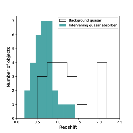
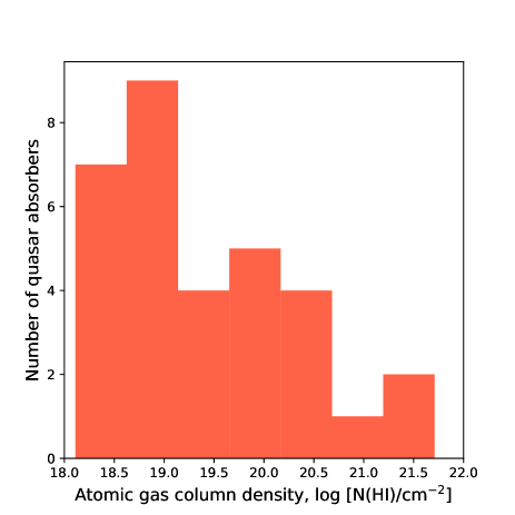
Figure 1: Quasars and primary targets properties. Left panel: Redshift distribution (in black) of the 19 background quasars making up the MUSE-ALMA Haloes survey. The filled histogram (green) displays the redshift distribution of the 32 intervening absorbers along the line-of-sight to these quasars, composing the primary target sample. Right panel: Atomic hydrogen gas column density distribution of these strong absorbers. The selection criterion imposes the cut at log [N(H I)/cm^-2]$>$18.

3.1 The Primary Targets

MUSE-ALMA Haloes is based on a unique selection of known quasar absorbers based solely on two criteria:

1. measured H i column density log [N(H I)/cm^-2]$>$18, from HST UV spectroscopy, which delivers spectra with resolutions R=20,000-30,000

2. $z_{\rm abs}<0.85$, to ensure that all emission lines up to [OIII] $\lambda$ 5007Å will be covered by the VLT/MUSE observations

MUSE-ALMA Haloes complements other surveys thanks to these key elements of the selection. The H i upper limits denote quasar absorbers with columns very near this limit, and in all cases, well above log [N(H I)/cm^-2]$>$15. The observations were undertook with either HST/FOS (Harms & Fitch, 1991), COS (Green et al., 2012) or STIS (Kimble et al., 1998). References to the published H i column density measurements are provided as a footnote to Table LABEL:tab:abs. Indeed, we stress that an accurate knowledge of H i column density in absorption is pivotal to a precise measure of neutral gas metallicity including a potentially required correction for the photoionised fraction of the gas. In addition, H i is a key ingredient in the estimate of the mass loading factor. The redshift range, which complements other efforts at $z>3$, is set to permit the robust determination of the systemic redshift based on narrow emission lines (as opposed to Ly$\alpha$), as well as the star formation rates and emission metallicity of these galaxies based on rest-frame optical emission diagnostics. Finally, the larger apparent size and surface brightness at these relatively modest redshifts compare to higher-redshifts enable a kinematic reconstruction of a large number of objects. The sample resulting from this selection comprises 32 individual absorbers (the "primary targets") in 19 unique fields. The $N(\mbox{\text{H\,{i}}})$ and redshifts of these systems are provided in Table LABEL:tab:abs. The distributions of their redshifts and H i columns are presented in Fig. 1.

The selected primary targets are well-studied strong absorbers. For this reason, they benefit from a number of addition ancillary data sets. By selection, all fields have high-resolution UV spectroscopy from HST. Most of the targets have ground-based optical high-resolution quasar spectra from VLT/UVES, X-Shooter or Keck/HIRES observations. These spectra provide abundance estimates based on the weaker metal lines of e.g. Si II, S II, Zn II and Cr II. One of the absorbers (towards Q1229$-$021) has also been detected in 21cm against the radio-loud background quasar as part of the FLASH survey currently on-going on ASKAP (Sadler et al., 2020). More of the MUSE-ALMA Haloes targets will also be part of FLASH’s Phase 2, potentially providing additional information on atomic gas kinematics and spin temperature. While this paper focuses on the newly acquired data, the ancillary observations will be presented in upcoming publications. The instruments used to record the high-resolution quasar spectra are also provided in Table LABEL:tab:abs.

3.2 Additional Absorbers

In addition to the primary targets, with log [N(H I)/cm^-2]$>$18, the sightlines to the background quasars contain a number of additional metal absorbers and higher-redshift systems. While these are not directly the targets of the primary sample, most of the science described in Section 2 is also addressed by these additional absorbers. These typically include MgII absorbers with log [N(H I)/cm^-2]$<$18 and associated with well-identified [OII] emitters observed with VLT/MUSE (see e.g. Rahmani et al., 2018b; Hamanowicz et al., 2020). We refer to this sample as the "additional absorbers".

3.3 The Galaxy-selected Sample

Beyond the absorber-selected targets, each of the 19 VLT/MUSE cubes contains several dozen $z_{\rm gal}<1.2$ galaxies with secure redshifts below the quasar redshift (typically $<z_{\rm quasar}>=1.2$). This additional sample includes 215 galaxies across all fields. These objects are selected independently of whether they are related to a known absorber, but they are at redshifts for which we have coverage in the existing quasar spectra to characterise the cold gas traced by e.g. Mg II absorbers. This provides a large sample of absorber-blind galaxies with a wealth of information about their physical properties. Indeed, statistically probing the physical properties of galaxies which do not have extended gaseous haloes is important to draw a full picture of the baryon cycle (Chen et al., 2021). Equally, the HST observations provide a measure of the stellar mass of several hundreds of galaxies, including numerous objects outside the VLT/MUSE field-of-view. We refer to this part of the survey as the "galaxy-selected sample". This larger dataset constitutes the main focus of the current paper. We note that by construction the primary sample is a subset of the galaxy-selected sample.

3.4 Supplementary Science Targets

In addition to the main science cases, the MUSE-ALMA Haloes data provide detailed information for 19 bright $0.48<z_{\rm quasar}<2.19$ quasars. The dataset includes high spatial resolution ($\sim$2kpc) observations of potential quasar-driven massive outflows thought to be omnipresent in bright quasar-host galaxies (Harrison et al., 2016, 2018). Moreover, MUSE-ALMA Haloes covers a large volume robust against cosmic variance, providing spectra and redshifts for hundreds of galaxies ranging from $z=0$ to $z=6.5$, including Ly$\alpha$ emitters at $z_{\rm gal}>3$.

4 Observing Strategy

4.1 Optical Integral Field Spectrograph VLT/MUSE Observations

The VLT/MUSE observations were carried out in service mode (under programmes ESO 96.A-0303, 100-A-0753, 101.A-0660 and 102.A-0370, PI: C. Péroux and 298.A-0517, PI: A. Klitsch) at the European Southern Observatory on the 8.2 m Yepun telescope. Each MUSE observations were centered on the bright background quasar. To optimise the schedulability of the runs, a mix of natural seeing mode and GALACSI Adaptive Optics (AO) system observations was used as indicated in Table LABEL:tab:JoO_MUSE. In addition, to ease the scheduling of the P100, P101 and P102 runs, we adopted a proven strategy tested during our early study of relaxing the observing conditions where the gain from AO is the highest. The resulting image quality (FWHM values) are listed in Table LABEL:tab:JoO_MUSE. The table also includes exposure times for each field observed. Each exposure was further divided into two equal sub-exposures, with an additional field rotation of 90 degrees and sub-arcsec dithering offset in 2-step pattern to minimise residuals from the slice pattern. The resulting field of view is 59.9 arcsec $\times$ 60 arcsec, with a 0.2 arcsec/pixel scale. We used the "nominal mode" resulting in a spectral coverage of $\sim$4800-9300 Å (Bacon et al., 2010). The AO-assisted observations are blind to wavelengths cut-out by the notch filter between 5820-5970 Å. The spectral resolution is R=1770 at 4800 Å and R=3590 at 9300 Å resampled to a spectral sampling of 1.25 Å/pixel. A journal of observations summarising the properties of the MUSE program is presented in Table LABEL:tab:JoO_MUSE.

Table 2: Journal of VLT/MUSE observations. The MUSE observations were carried out in service mode over various observing campaigns with a combination of natural seeing and GALACSI Adaptive Optics (AO) system modes. The $3\sigma$ line flux limits are calculated at $7000$ Å for an unresolved source spread over a disk with diameter equal to the seeing and with FWHM $=3$ Å.

Quasar	$t_{\rm exp}$	AO?	I.Q.a	Flux limit	Prog. ID	PI	MUSE-ALMA Haloes
field	[s]		["]	[$\text{erg s}^{-1}\text{cm}^{-2}$]			references
Q0058$+$0019	1410+330	AO	1.23	2.8$\times 10^{-17}$	102.A-0370	Péroux	this work
Q0123$-$0058	1410$\times$2	no	2.11	5.5$\times 10^{-17}$	100.A-0753	Péroux	this work
Q0138$-$0005	1410$\times$2	AO	1.11	3.6$\times 10^{-17}$	101.A-0660	Péroux	this work
J0152$-$2001	1200$\times$4	no	0.72	4.7$\times 10^{-18}$	096.A-0303	Péroux	Rahmani et al. (2018a, b)
Q0152$+$0023	1410$\times$2	AO	0.65	1.2$\times 10^{-17}$	101.A-0660	Péroux	this work
Q0420$-$0127	1405$\times$4	no	0.71	4.0$\times 10^{-18}$	298.A-5017	Klitsch	Klitsch et al. (2018)
Q0454$+$039	1410$\times$4	no	0.81	5.3$\times 10^{-18}$	100.A-0753	Péroux	this work
Q0454$-$220	1410$\times$2	no	0.57	2.3$\times 10^{-18}$	100.A-0753	Péroux	this work
Q1110$+$0048	1410$\times$2	AO	0.52	2.6$\times 10^{-18}$	101.A-0660	Péroux	this work
J1130$-$1449	1200$\times$6+960$\times$2	no	0.76	4.2$\times 10^{-18}$	096.A-0303	Péroux	Péroux et al. (2019)
J1211$+$1030	1200$\times$4	no	0.75	6.8$\times 10^{-18}$	096.A-0303	Péroux	Hamanowicz et al. (2020)
Q1229$-$021	1200$\times$4	no	0.80	7.3$\times 10^{-18}$	096.A-0303	Péroux	Hamanowicz et al. (2020)
Q1342$-$0035	1410$\times$2	AO	1.30	2.0$\times 10^{-17}$	101.A-0660	Péroux	this work
Q1345$-$0023	1410$\times$2	AO	0.64	4.8$\times 10^{-18}$	101.A-0660	Péroux	this work
Q1431$-$0050	1410$\times$2	AO	0.54	7.1$\times 10^{-18}$	101.A-0660	Péroux	this work
Q1515$+$0410	1410$\times$4	AO	0.59	5.2$\times 10^{-18}$	101.A-0660	Péroux	this work
Q1554$-$203	1410$\times$4	AO	0.79	6.0$\times 10^{-18}$	101.A-0660	Péroux	this work
J2131$-$1207	1200$\times$4	no	0.72	4.6$\times 10^{-18}$	096.A-0303	Péroux	Péroux et al. (2017); Szakacs et al. (2021a)
Q2353$-$0028	1410$\times$4	AO	0.81	5.2$\times 10^{-18}$	101.A-0660	Péroux	this work

Note: ^a I.Q. refers to the image quality in the reconstructed cube measured from a Gaussian fit at 7000 Å.

4.2 ALMA mm Observations

The ALMA data included in the MUSE-ALMA Haloes survey are comprised of three distinct catalogues: i) proposals led by our group, ii) targets included in ALMACAL and iii) archival data.

Firstly, a subset of the quasar fields were observed with ALMA specifically for use in the MUSE-ALMA Haloes survey. The details of these runs are described in Péroux et al. (2019); Klitsch et al. (2021); Szakacs et al. (2021a) and we only give a brief overview here. The observations were performed in Bands 3, 4 or 6 and covered the CO(1–0), CO(2–1) or CO(3–2) emission lines at the redshift of the primary targets. The programmes were 2016.1.01250.S and 2017.1.00571.S (PI: C. Péroux) and 2018.1.01575.S (PI: A. Klitsch). The precipitable water vapour (PWV) for these observations varied between 0.65 and 5.4 mm and the total on-source observing times are listed in Table LABEL:tab:JoO_ALMA. The data were observed in relatively compact antenna configurations which resulted in an angular resolution of the order 1″. For each target, one of the four spectral windows was centred on the redshifted CO line frequency and used relatively high spectral resolution (4096 dual-polarization channels across a bandwidth of 1875 MHz) whilst the other three spectral windows were used to observe the continuum and thus only required 128 channels each over the same bandwidth.

Second, some of the MUSE fields are part of the ALMACAL survey. ALMACAL is an ingenious mm survey that exploits ALMA phase and amplitude calibration data. Since 20 per cent of all ALMA telescope time has been spent on calibrators, ALMACAL is already the widest and deepest mm survey. The amount of data processed to date adds up to over 2000 hrs of ALMA observation time, equivalent to about half of all observing time awarded to observers in a one-year ALMA cycle. These data become publicly available immediately, without proprietary time. This calibrator survey can be used to study both the calibrators themselves and any serendipitously-detected galaxies in the field. One of the fields (namely Q0420$-$0127) had already appropriate frequency coverage and sufficient depth to enable a detailed study (Klitsch et al., 2018). As ALMA is observing repeatedly the same calibrator fields, further data will likely become available in the future.

Thirdly, data for four of the targets are available in the ALMA archive, two of which (Q0058$+$0019 and Q0138$-$0005) were previously published (Kanekar et al., 2018).

A journal of observations summarising the properties of the ALMA runs as of July 15^th 2022 is presented in Table LABEL:tab:JoO_ALMA. The table includes exposure times, spatial resolution, primary beam diameter and frequency coverage.

Table 3: Journal of ALMA observations. "PI data" are from our group, "ALMACAL" means that the target is observed as an ALMA calibratorand "archive" refers to the general ALMA archive (shown in italics) as of July 15th 2022. "…" refers to entry with no ALMA observations.

Quasar	$t_{\rm exp}$	Catalogue	Resolution	ALMA	Primary	Frequency	Cont.	Prog. ID	PI	References
field				Band	Beam	cov	Sens
	[min]		["]		["]	[GHz]	[mJy]
Q0058$+$0019	41	archive	1.61	4	44	129.91-145.89	0.014	2013.1.01178.S	Prochaska	Kanekar et al. (2018)
…	66	archive	1.76	4	44	129.97-145.89	0.017	2015.1.01034.S	Prochaska	Kanekar et al. (2018)
Q0123$-$0058	…	…	…	…	…	…	…	…	…	…
Q0138$-$0005	12	archive	1.63	4	44	128.43-143.99	0.029	2013.1.01178.S	Prochaska	Kanekar et al. (2018)
…	32	archive	0.08	4	44	128.43-143.99	0.013	2015.1.01034.S	Prochaska	Kanekar et al. (2018)
J0152$-$2001	118	PI data	0.90	6	27	232.08-251.05	…	2017.1.00571.S	Péroux	Szakacs et al. (2021a)
Q0152$+$0023	…	…	…	…	…	…	…	…	…	…
Q0420$-$0127	1303	ALMACAL	1.75	3	62	84.03-115.88	0.0035	…	…	…
…	260	ALMACAL	0.77	4	44	125.03-162.88	0.0071	…	…	Klitsch et al. (2018)
…	256	ALMACAL	1.29	5	33	163.28-207.54	0.010	…	…	…
…	2167	ALMACAL	0.57	6	27	211.09-274.99	0.0050	…	…	Klitsch et al. (2018)
…	1332	ALMACAL	0.35	7	18	277.00-685.56	0.0078	…	…	…
…	162	ALMACAL	0.25	8	12	396.50-498.65	0.0090	…	…	…
…	20	ALMACAL	0.19	9	9	657.66-694.75	0.5	…	…	…
…	2.5	archive	1.76	3	62	88.20-90.69	2.3	2015.1.00503.S	Bronfman	…
…	4.5	archive	1.13	3	62	112.51-115.89	3.1	2015.1.00503.S	Bronfman	…
…	7.5	archive	1.79	3	62	88.25-91.13	1.2	2019.1.00743.S	Finger	…
…	2.0	archive	2.22	3	62	113.06-115.64	3.5	2019.1.00743.S	Finger	…
Q0454$+$039	…	…	…	…	…	…	…	…	…	…
Q0454$-$220	…	…	…	…	…	…	…	…	…	…
Q1110$+$0048	…	…	…	…	…	…	…	…	…	…
J1130$-$1449	227	PI data	1.07	3	62	86.88-102.80	0.0098	2016.1.01250.S	Péroux	Péroux et al. (2019)
…	57	ALMACAL	0.79	3	62	85.91 -113.63	0.018	…	…	…
…	19	ALMACAL	1.01	4	44	131.57-151.98	0.029	…	…	…
…	8	ALMACAL	0.98	6	27	211.98-245.83	0.057	…	…	…
…	9	ALMACAL	0.29	7	18	335.50-358.93	0.080	…	…	…
J1211$+$1030	45	PI data	0.69	6	27	231.99-250.97	0.014	2017.1.00571.S	Péroux	Szakacs et al. (2021a)
Q1229$-$021	293	PI data	0.99	6	27	246.95-265.99	0.018	2017.1.00571.S	Péroux	Szakacs et al. (2021a)
…	50	ALMACAL	1.91	3	62	89.44 -115.08	0.016	…	…	…
…	34	ALMACAL	0.41	6	27	213.99-266.70	0.022	…	…	…
…	3	ALMACAL	0.14	7	18	335.50-351.48	0.071	…	…	…
…	3	archive	0.67	6	27	223.01-242.99	0.052	2015.1.00932.S	Meyer	…
…	1	archive	0.89	3	62	89.50-105.48	0.059	2016.1.01481.S	Meyer	…
…	2	archive	0.44	6	27	222.99-242.97	0.062	2016.1.01481.S	Meyer	…
…	4	archive	0.35	3	62	89.50-105.48	0.035	2015.1.00932.S	Meyer	…
…	7	archive	0.20	6	27	223.03-243.01	0.032	2016.1.01481.S	Meyer	…
…	4	archive	0.22	3	62	89.51-105.49	0.030	2016.1.01481.S	Meyer	…
Q1342$-$0035	…	…	…	…	…	…	…	…	…	…
Q1345$-$0023	…	…	…	…	…	…	…	…	…	…
Q1431$-$0050	…	…	…	…	…	…	…	…	…	…
Q1515$+$0410	…	…	…	…	…	…	…	…	…	…
Q1554$-$203	…	…	…	…	…	…	…	…	…	…
J2131$-$1207	120	PI data	0.97	6	27	224.00-242.80	0.013	2017.1.00571.S	Péroux	Szakacs et al. (2021a)
…	6	PI data	0.65	4	44	146.55-162.17	0.033	2018.1.01575.S	Klitsch	Klitsch et al. (2021)
…	4	ALMACAL	1.09	3	62	88.36 -105.49	0.022	…	…	…
…	10	ALMACAL	0.78	6	27	213.53-269.93	0.011	…	…	…
…	2	ALMACAL	0.46	7	18	335.50-351.49	0.090	…	…	…
Q2353$-$0028	…	…	…	…	…	…	…	…	…	…

4.3 HST Broad-Band Imaging

MUSE-ALMA Haloes also includes broad-band imaging of most of the fields in the sample. The new data were observed during Cycle 27 as part of a 40-orbit medium programme (ID: 15939; PI: C. Péroux) with the Wide Field Camera 3 in both the optical (UVIS) and infrared (IR) detectors, using different combination of broad-band filters as indicated in Table LABEL:tab:JoO_HST. We also make use of archival data recorded with WFPC. Together, the observations took place between January 2015 and May 2021. For the dedicated programme, we aimed at setting the roll-angle of the telescope such that the primary target galaxy counterpart revealed by MUSE lies at 45 degrees from the diffraction spikes of the instrument Point Spread Function (PSF). We use a dithering pattern in four individual exposures to help with removal of cosmic rays and hot pixels. The UVIS observations were initially taken using the WFC3-UVIS-DITHER-BOX pattern. The two observations with the IR detector were taken using the WFC3-IR-DITHER-BOX-MIN pattern providing an optimal 4-point sampling of the PSF. Some of the observations failed due to HST pointing drifts and only a fraction of these fields were reobserved. In these cases, the dithering pattern might differ slightly. For some fields, we also rely on existing archival data to constrain the galaxy spectral energy distribution (SED) on either side of the 4000 Å Balmer break. The majority (16/19) of the fields have three broad-band filters available. Using additional data available in the HST archive, we even cover a total of 4 filters for some of the targets. A summary of the observational set-up, including observing times, is given in Table LABEL:tab:JoO_HST.

Table 4: Journal of HST Observations. The broad-band imaging observations available from the Space Telescope Science Institute archive are shown in italics. In the cases of several primary targets in the field, the chosen broad-band filters are well suited to probe the wavelength range bluewards of the 4000Å break. "…" refers to entry with no HST observations.

Quasar field	texp	HST	Central $\lambda$	Mag	Prog. ID	PI
	[s]	camera/filter	[Å]	Limit
Q0058$+$0019	27676	WFPC F702W	6919	27.02	6557	Steidel
Q0123$-$0058	…	…	…	…	…	…
Q0138$-$0005	2367	WFC3/UVIS F475W	4774	28.70	15939	Péroux
…	2364	WFC3/UVIS F625W	6242	28.90	15939	Péroux
…	2412	WFC3/IR F105W	10557	27.93	15939	Péroux
J0152$-$2001	2364	WFC3/UVIS F336W	3355	29.39	15939	Péroux
…	2364	WFC3/UVIS F475W	4774	29.29	15939	Péroux
…	1250	WFPC F702W	6919	27.68	6557	Steidel
Q0152$+$0023	2106	WFC3/UVIS F336W	3355	28.54	15939	Péroux
…	2489	WFC3/UVIS F475W	4774	28.39	15939	Péroux
…	2489	WFC3/UVIS F814W	8033	27.92	15939	Péroux
Q0420$-$0127	2122	WFC3/UVIS F336W	3355	28.30	15939	Péroux
…	2216	WFC3/UVIS F475W	4774	29.52	15939	Péroux
…	1918	NICMOS F160W	1607	24.12	7451	Smette
Q0454$+$039	2416	WFC3/UVIS F625W	6242	28.72	15939	Péroux
…	2000	WFPC F450W	4556	26.58	5351	Bergeron
…	3600	WFPC F702W	6919	27.97	5351	Bergeron
…	767	NICMOS F160W	1607	24.25	7329	Malkan
Q0454$-$220	2164	WFC3/UVIS F336W	3355	29.31	15939	Péroux
…	2564	WFC3/UVIS F475W	4774	29.34	15939	Péroux
…	1200	WFPC F702W	6917	26.02	5098	Burbidge
Q1110$+$0048	1500	WFC3/UVIS F336W	3355	29.56	15939	Péroux
…	1200	WFC3/UVIS F475W	4774	28.92	15939	Péroux
…	1200	WFC3/UVIS F814W	8033	27.45	15939	Péroux
J1130$-$1449	2152	WFC3/UVIS F336W	3355	29.42	15939	Péroux
…	2552	WFC3/UVIS F438W	4326	29.08	15939	Péroux
…	22000	WFPC F814W	8012	28.65	9173	Bechtold
…	2120	WFC3/IR F140W	1392	28.02	14594	Bielby
J1211$+$1030	2224	WFC3/UVIS F336W	3354	28.47	15939	Péroux
…	2000	WFPC F450W	4556	28.21	5351	Bergeron
…	3600	WFPC F702W	6919	27.43	5351	Bergeron
Q1229$-$021	2396	WFC3/UVIS F336W	3355	28.67	15939	Péroux
…	2000	WFPC F450W	4556	26.93	5351	Bergeron
…	4800	WFPC F702W	6919	27.55	5351	Bergeron
Q1342$-$0035	2106	WFC3/UVIS F336W	3355	28.54	15939	Péroux
…	2489	WFC3/UVIS F475W	4774	29.20	15939	Péroux
…	2489	WFC3/UVIS F814W	8033	28.12	15939	Péroux
Q1345$-$0023	500	WFC3/UVIS F336W	3355	28.68	15939	Péroux
…	600	WFC3/UVIS F475W	4774	29.56	15939	Péroux
…	1200	WFC3/UVIS F814W	8033	27.80	15939	Péroux
Q1431$-$0050	2106	WFC3/UVIS F336W	3355	29.06	15939	Péroux
…	2489	WFC3/UVIS F475W	4774	28.79	15939	Péroux
…	2489	WFC3/UVIS F814W	8033	28.08	15939	Péroux
Q1515$+$0410	2106	WFC3/UVIS F336W	3355	29.14	15939	Péroux
…	2489	WFC3/UVIS F475W	4774	29.62	15939	Péroux
…	2489	WFC3/UVIS F814W	8032	26.82	15939	Péroux
Q1554$-$203	2411	WFC3/UVIS F475W	4774	29.87	15939	Péroux
…	2576	WFC3/UVIS F625W	6242	28.89	15939	Péroux
…	2176	WFC3/IR F105W	10557	28.64	15939	Péroux
J2131$-$1207	2156	WFC3/UVIS F336W	3355	29.07	15939	Péroux
…	2556	WFC3/UVIS F475W	4774	29.26	15939	Péroux
…	1800	WFPC F702W	6919	27.22	5143	Macchetto
Q2353$-$0028	2106	WFC3/UVIS F336W	3355	29.48	15939	Péroux
…	2489	WFC3/UVIS F475W	4774	29.45	15939	Péroux
…	2489	WFC3/UVIS F814W	8033	27.78	15939	Péroux

5 MUSE-ALMA Haloes Data Processing

5.1 Optical Integral Field Spectrograph VLT/MUSE Cubes

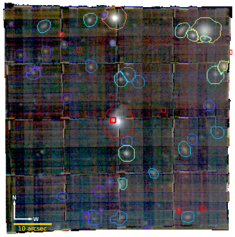
Figure 2: Example VLT/MUSE reconstructed RGB-colour image. Reconstructed AO-assisted image of the combined exposures of the field of Q1110$+$0048 collapsed along the wavelength axis. The total field-of-view is 59.9×60 arcsec². The total exposure time t_exp=1410 s$\times$2 and the resulting image quality of the combined datacube is FWHM=0.52 arcsec measured at 7000 Å. The quasar, with $z_{\rm quasar}$=0.76, is at the centre of the image. The objects visible in the field are bright in continuum. The colour contours illustrate of the automatically-generated segmentation map in the Johnson R-band of the same field ordered in terms of increasing flux. Brighter objects are warmer colours (red/orange) whereas fainter objects are blue/violet. Such segments are used to estimate the magnitudes of the sources in multiple bands with the ProFound R Package. The objects marked by small red squares are not continuum-detected but identified through their emission lines with the mpdaf/MUSELET package. The red square underneath the quasar PSF is also detected in HST observations (see Fig. 3). VLT/MUSE observations additionally provide spectroscopic and kinematic information for the majority of the objects in the field.

The data were reduced with the ESO MUSE pipeline (Weilbacher, 2015) and additional external routines for sky subtraction and extraction of the 1D spectra. Master bias, flat field images and arc lamp exposures based on data taken closest in time to the science frames were used to correct each raw cube. We checked that the flat-fields are the closest possible to the science observations in terms of ambient temperature to minimise spatial shifts. In all cases, we found the temperature difference to be below the canonical 0.5 degrees set to be the acceptable limit. Bias and flat-field correction are part of the ESO pipeline. The raw science data were then processed with the $scibasic$ and $scipost$ recipes. During this step, the wavelength calibration was corrected to a heliocentric reference. We note that MUSE operates in air, not vacuum. We checked the wavelength solution using the known wavelengths of the night-sky [O i] and OH lines across the wavelength coverage of MUSE. We find a median discrepancy of $25$ km/s in the wavelength solution across the fields. The individual exposures were registered using the point sources in the field within the $exp\_align$ recipe, ensuring accurate relative astrometry. The astrometry of HST/WFC3 is checked using the central quasar as reference, and it is found to be accurate within sub-arcsec. Finally, the individual exposures were combined into a single data cube using the $exp\_combine$ recipe. The image quality of the final combined data is measured from a gaussian fit of the quasar at 7000Å in the data cube. The resulting PSF FWHM values are listed in Table LABEL:tab:JoO_MUSE.

To estimate flux errors, we measured fluxes in synthetic VLT/MUSE broad-band images created by applying HST filter curves, and then compared these measured pseudo magnitudes to the actual HST data. While we refrain from systematically correcting the MUSE flux levels in order to keep information on the associated uncertainties, on four occasions (Q0138$-$0005, Q0152$+$0023, Q1431$-$0050 and Q1515$+$0410) where the flux differences were large ($>$50 per cent) we adjusted the MUSE flux levels so as to match the HST values. In addition, for fainter objects ($>23$ mag), we applied an additional error correction due to the volatility in the MUSE magnitudes (Roth et al., 2018). The standard deviation of the magnitude difference between MUSE and HST fluxes is added in quadrature to the error term returned by ProFound to obtain the final magnitude error. For the field without optical or near-IR HST data, we compared the measured fluxes of the central quasar and bright stars from pseudo Cousins V, Johnson R and SDSS r and i images with literature values. Overall, we estimate the uncertainties to be on average $\pm 30$ per cent. Finally, we checked the VLT/MUSE absolute astrometry using the HST/WFC3 data when available. We applied appropriate systemic offsets of the order 1 arcsec to the VLT/MUSE cubes.

The removal of OH emission lines from the night sky is accomplished with additional purpose-developed codes. The $scipost$ recipe is first performed with sky-removal method "simple" on, which directly subtracts a sky spectrum created from the data, without regard to the line spread function (LSF) variations. After selecting sky regions in the field, we create Principal Component Analysis (PCA) components from the spectra which are further applied to the science datacube to remove sky line residuals (Husemann et al., 2016; Péroux et al., 2017). This method is required as an addition to the ESO pipeline to significantly improve the sky subtraction over large parts of the MUSE field-of-view. The RGB-colour image of an example field is shown in the left panel of Fig. 2.

5.2 ALMA mm Cubes

We describe here the steps taken to reduce the ALMA data. Additional details can be found in Péroux et al. (2019); Szakacs et al. (2021a); Klitsch et al. (2021) for the PI data and Klitsch et al. (2018) for ALMACAL. We started the data reduction with the pipeline-calibrated $u,v$ data as delivered by ALMA. Additional data reduction steps were carried out with the Common Astronomy Software Applications (CASA) software package. Minor manual flags were added to remove some $u,v$ data with strongly outlying amplitudes. Some of the quasar in the centre of the science fields are very bright at mm frequencies ($\geq$100 mJy), which makes them ideal sources for self-calibration, in both amplitude and phase.

Self-calibration was carried out by firstly using tclean to Fourier transform the $u,v$ data into a continuum image and deconvolving. Self-calibration was then performed using the gaincal and applycal on individual measurement sets to produce corrected $u,v$ data, after which the data were re-imaged to create an improved continuum map. We applied one round of phase self-calibration and one round of amplitude and phase self-calibration. The next step was to subtract the bright continuum source from the field using the uvsub. We then created a cube with tclean, setting the pixel size so as to oversample the beam sufficiently and using a ‘robust’ weighting scheme with a Briggs parameter of 0.5 or 1. Residual continuum signatures around the imperfectly subtracted quasar were removed using uvcontsub. After searching for emission lines, we corrected the cube for the primary beam using pbcor in order to correctly measure their flux. We note that the resulting FWHM of the primary beam of ALMA in Band 3 is $\sim$62″, conveniently matching the VLT/MUSE field-of-view. We refer the reader to Klitsch et al. (2018); Péroux et al. (2019); Klitsch et al. (2021); Szakacs et al. (2021a) for examples of the resulting ALMA datacubes.

5.3 HST Broad-Band Imaging

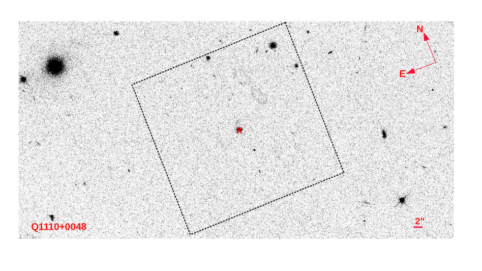
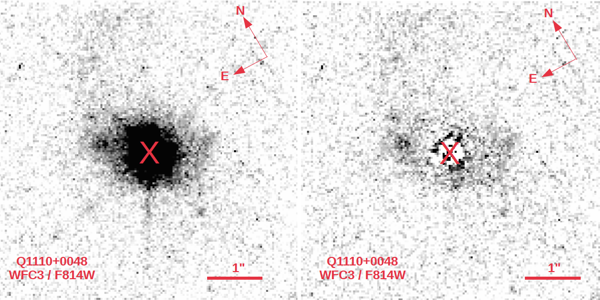
Figure 3: Example HST broad-band imaging. Reconstructed image of the combined exposures of the field of Q1110$+$0048 in the F814W UVIS filter-band. The total exposure time t_exp is 1200 sec. The quasar, with $z_{\rm quasar}$=0.76, is at the centre of the images and is marked with a red cross. Top panel: The full F814W UVIS broad-band image. The MUSE field-of-view is overlaid as a dotted square. The image shows multiple objects which are bright in continuum. Bottom left panel: Zoom-in of the same image. The bright quasar displays strong diffraction spikes. Bottom right panel: Same zoom-in image after a careful PSF-subtraction has been performed to remove the quasar image as described in the text. The image clearly shows an additional object north-east of the quasar, which is also detected in emission in the VLT/MUSE cube (see Fig. 2).

5.3.1 Data Reduction

The WFC3 data were reduced with the calwf3 pipeline. The pipeline processing steps include bias subtraction, dark subtraction, and flat fielding. Each individual reduced exposure was multiplied by the pixel area map provided on the HST/WFC3 photometry website in order to perform flux calibration. Bad pixels, saturated pixels, and pixels affected by cosmic rays were masked using the data quality file provided with each science frame. Subpixel grids were constructed on the individual exposures for the purpose of achieving accurate alignment of dithered images, using grids of 5$\times$5 pixels for the full images, and 10$\times$10 pixels for the central portions of the images zoomed in on the quasar. The individual sub-pixeled images were sky-subtracted and then shifted with respect to each other as needed to align them. In some cases, the individual exposures were taken at different roll angles, resulting in relative rotation of the field. In such cases, the tasks Tweakreg and Astrodrizzle were used to rotate the images before alignment. The sky-subtracted, aligned individual exposures were then median-stacked to produce the final science images. The upper panel of Fig. 3 shows an example WFC3 UVIS image for one of the fields in the filter F814W.

The archival WFPC data were reduced with the calwp2 pipeline, which includes the steps of bias subtraction, dark subtraction, and flat field correction. The data quality file provided with each science data file was used to flag bad pixels and saturated pixels. The IRAF task CRREJ was used to correct pixels hit by cosmic rays in each science frame. The resulting images were further processed using identical steps as described above for WFC3 data (subpixeling and sky-subtraction of the individual dithered exposures, alignment of the individual images including rotation with Tweakreg and Astrodrizzle if necessary, and median stacking of the aligned images). We note that in the two cases where rotational alignment using Tweakreg and Astrodrizzle was performed, the multiplication by pixel area map was not performed, since the varied pixel area is fixed by the drizzle process. In all other cases, the multiplication by the pixel area map was necessary since the FLC images were used directly.

5.3.2 Subtraction of Quasar Point Spread Function

The primary difficulties in detecting in emission the galaxy or galaxies producing a quasar absorption system are the faintness of the galaxy relative to the background quasar and the small angular separation between the galaxy and the quasar. To make it possible to detect the galaxy’s continuum emission, it is essential to remove the contamination from the quasar by subtracting the point spread function (PSF) from the quasar image. A major advantage of HST, in this context, over ground-based imaging systems is that the PSF of HST cameras is far better defined and stable compared to the PSFs of ground-based imaging systems (even those using adaptive optics). Of course, given the diffraction-limited nature of HST imaging, the PSF depends on the wavelength of observation, and is thus different for different filters. Moreover, the PSF can vary spatially across the field of view. Guided by our past experience with PSF subtraction for detecting galaxies in quasar fields (e.g. Kulkarni et al., 2000, 2001; Chun et al., 2010; Straka et al., 2011; Augustin et al., 2018), we constructed the PSF using our own observations, rather than relying on theoretical PSF models. For constructing the PSF in each filter for each quasar field, we used observations of all other quasar fields from our sample in that same filter, combining all such observations after masking objects other than the central quasars, subtracting the sky from each image, aligning the different images spatially so that the diffraction spikes overlap, and scaling them as needed in flux to make the flux levels match in the outer wings of the PSF. The such reconstructed PSF was then aligned and matched in flux with the studied quasar and subtracted from the quasar to reveal any underlying galaxies. This strategy proved successful, and led to robust removal of diffraction spikes, enabling detections of faint galaxies previously hidden under the quasar PSF in several of our fields. A similar approach was adopted while performing the PSF subtraction for the archival WFC3 or WFPC images, constructing the PSF from either an isolated star in the field or from a combination of different quasar images in the same filter. The lower two panels of Fig. 3 demonstrate the effectiveness of our PSF subtraction strategy. While the residual flux level close to the subtracted quasar’s centre (marked with an “X") is not always zero, it is possible to see faint extended objects which were hidden under the PSF a little further away from the quasar centre.

6 Searching for Extra-galactic Objects

The identification of galaxies in our data is necessary to explore the cosmic baryon cycle. We used the VLT/MUSE observations of the quasar fields, together with the HST wide-field broad-band imaging to search for all extra-galactic objects in each field. Several analysis techniques were applied to maximize the completeness of the search of different types of objects (star forming-galaxies, passive galaxies, faint objects etc.). VLT/MUSE datacubes can be viewed as individual narrow-band (NB) images at each wavelength slice or a combined continuum image over the whole observed wavelength range, allowing for two types of object searches in the data: a single spectral-line search and identification of the sources seen in continuum.

6.1 Detecting Emitting Galaxies in VLT/MUSE Cubes

We expect the presence in the VLT/MUSE data of objects with emission lines but no detectable continuum. Some of these sources may only exhibit a single emission line and the interpretation of these sources requires further inspection. We used the MUSE Line Emission Tracker (MUSELET) module of the MPDAF package (Piqueras et al., 2017) to systemically search for emission-line objects. MUSELET creates synthetic narrow-band images (width of $7.25$ Å) at each wavelength plane of a cube that are then passed through SExtractor to find objects with emission lines. Regions near the night sky emission lines at $5577$ and $6300$ Å were excluded to limit the number of false detections caused by residues from the sky subtraction. The list of objects from MUSELET will overlap with the continuum objects detected, and these were removed to prevent duplicates.

In some cases, we detected galaxies close to the quasar position (within 1 arcsec), blended with the quasar PSF. In order to uncover such object, we performed a careful spectral PSF subtraction within QFitsView. To this end, the quasar PSF was fitted as a function of wavelength so that it became possible to detect faint emitting galaxies despite the bright quasar contribution. This technique however provides limited information on the continuum properties of such galaxy (although see Rupke et al., 2017; Helton et al., 2021).

6.2 Detecting Continuum Galaxies in VLT/MUSE Cubes

The ProFound R Package (Robotham et al., 2018) was used to detect continuum sources in the MUSE fields. First, white-light and synthetic Cousins V, Johnson R and SDSS r and i band images were created using MPDAF. ProFound was initially used on the white-light image to produce a preliminary segmentation map. Due to background residuals in some fields, the $profoundSegimFix$ function was used to manually modify affected segments and remove false detections (Bellstedt et al., 2020; Foster et al., 2021). An example segmentation map is shown in Fig. 2 for illustration. Finally, ProFound was run in multi-band mode to determine the photometric properties in the V, R, r and i bands by collapsing the MUSE cubes in wavelength ranges specific to different bands.

The choice of ProFound over SExtractor stems from the difference in nature between the VLT/MUSE white-light images and HST broad-band images. While objects in the HST images are typically separated due to the lower PSF FWHM, the blending of adjacent objects occurs in our VLT/MUSE fields. This increases the importance of obtaining accurate segmentation maps by ensuring apertures do not erroneously combine segments, which was seen to occur more often in SExtractor (Wright et al., 2016; Robotham et al., 2018). Both programs were used to search for continuum sources and it was found that ProFound produced more accurate segmentation maps. For bright and isolated point sources, the photometric properties measured using both alogrithms were found to be consistent within $5$ per cent.

Last, we also used HST detection of faint continuum sources as prior information for assessing the VLT/MUSE possible sources. The sky position of the HST objects were used as priors to extract spectra from the VLT/MUSE cubes which were then processed in the same way as any other continuum detected objects. This process led to a couple of additional detections.

6.3 Detecting Continuum Galaxies in HST Broad-Band Imaging

The Astropy package Photutils was used on the processed HST broad-band images in each filter for each field to search for all objects and to perform photometry of the detected objects. Apertures were optimised by repeating the photometry on elliptical apertures of increasing sizes for each object and adopting the aperture size beyond which the flux of that object stayed constant (taking care to check that the aperture did not include multiple objects). Because this was done separately for each band, we also checked the aperture corrections. To this end, we estimated the Sersic index and the effective radius of the objects using GALFIT. We next computed the theoretical light profile for the Sersic index and the effective radius thus determined. Using this profile, we examined the flux enclosed within apertures of radius $r$ (i.e., flux integrated from 0 to $r$) as a function of $r$. We then determined the minimum radius above which the enclosed flux remains constant (i.e., stops increasing). We find that this radius is less than the one used in both SExtractor and ProFound, indicating that the aperture corrections are negligible and the magnitudes of the aperture corrections are comparable for the different bands. The package SExtractor was used to classify each object detected in the field as a star or a galaxy using the CLASS$\_$STAR parameter in SExtractor. As an additional check on the photometry, fluxes computed using SExtractor were compared with those obtained using Photutils, and were found to agree closely (within $\sim$2-5 per cent). Once the photometry in each filter was completed, cross-matching was performed between the objects detected in the different filters using the tool Topcat (Taylor, 2005), to construct a catalog of all detected objects in each field, including the photometry for each object in all filters. In cases where an object detected in one filter was not detected in another filter, a 3-$\sigma$ magnitude limit was calculated for the filter with the non-detection by measuring the 3-$\sigma$ noise level (over the number of pixels occupied by the object in the filter with the detection). Finally, the objects in the catalog were examined visually to identify any spurious detections near the edges of the images (caused by artifacts), and such false objects were removed from the catalog.

7 Galaxies’ Physical Properties

7.1 Optical Spectral Extraction

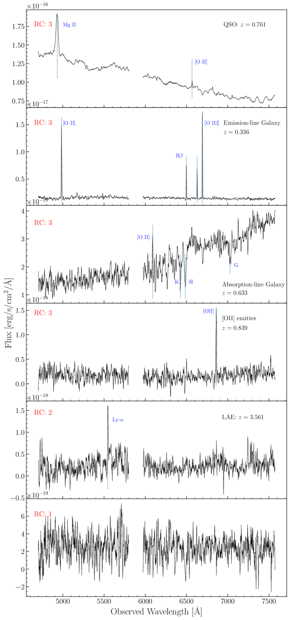
Figure 4: Example VLT/MUSE spectra. Five-pixel boxcar/moving-average spectra of six objects observed as part of the Q1110$+$0048 VLT/MUSE cube. The assigned spectral redshift confidence ("RC") is given in red at the top left of each panel. The [O ii] emitter at $z=0.839$ in the fourth panel from the top has its doublet resolved in the unsmoothed spectrum and hence, it was graded as a ’redshift confidence: 3’. The wavelengths not plotted correspond to the notch filter between 5820-5970 Å inherent to AO-assisted observations. The spectral resolution is R=1770 at 4800 Å and R=3590 at 9300 Å resampled to a spectral sampling of 1.25 Å/pixel.

The spectral extraction method differs for the continuum objects detected using ProFound and emission-line objects found by MUSELET. Due to the large variability in seeing conditions between the fields, the ideal aperture size for extracting the spectra of our continuum sources will differ significantly across cubes. Additionally, objects within cubes have varying sizes and morphologies. To obtain the optimal spectra for for redshift determination in each field, a range of circular apertures with sizes ranging from $0.3$ to $2.0$ arcsec in radius was used. The lower limit is set by the PSF FWHM of the MUSE data cube and all the apertures have a minimum diameter above this value. For each aperture radius, the signal-to-noise (S/N) of the spectrum at the wavelength interval spanning $\sim 5000-5200$ Å  was calculated. This wavelength region is chosen as there are no night sky emission lines or artefacts in this range, and the aperture size where S/N is maximised determined our final extracted spectrum. Redder wavelength planes ($7050-7200$ and $8100-8250$ Å) were also tested and the change in S/N consistently varied with aperture size across the different wavelengths. To prevent our apertures from including neighbouring objects, regions outside the segment containing the object are masked. While the apertures used are circular, masking based on the segmentation map effectively changes the aperture shape to the shape of the segment and by extension, our object. While these are not the spectra used for emission lines flux measurement, we note that $>95$% of an object’s total flux is captured using this method to extract spectra.

For the emitters detected by MUSELET and sources extracted using the broad-band HST images as a prior, a circular aperture of radius $0.5$ arcsec is used to obtain spectra. These objects are not expected to be detected in continuum and hence the choice of aperture size becomes less relevant. Example VLT/MUSE spectra are displayed in Fig. 4.

7.2 Spectral Classification

The extracted VLT/MUSE spectra are used to both identify the sources and to estimate the redshift of extra-galactic objects. To this end, we use the MARZ tool (Hinton et al., 2016) with the M. Fossati fork. This fork includes additional high-redshift templates and high-resolution templates well suited for VLT/MUSE data. MARZ provides both a visualisation tool and a template cross-correlation tool for each source with quasar, galaxy and stellar template spectra. The results are visually inspected by two experts (SW and CP) to confirm the nature and redshift of the source based on continuum level and shape as well as on detected emission and absorption lines. Faint sources can have spectra of insufficient quality to attempt a redshift determination using cross-correlations, though some have bright emission lines and are included in the catalogue following the search for emission lines described earlier. The redshift success rates ranges from 100% at $r_{\rm mag}=20$ down to typically 60% at $r_{\rm mag}\sim 25$.

We therefore provide redshift confidences for each source. They are as follows: (1) spectra without emission or absorption features and no redshift estimate is possible, (2) a redshift measure is possible as the spectra contains low S/N emission and absorption lines, and (3) a robust redshift is determined where there is a high S/N emission line that is clearly resolved [OII] doublet or asymmetric Lyman-$\alpha$, one high S/N emission line with other fainter absorption or emission features, or with multiple clear emission and/or absorption lines, and finally (6) stellar objects. These results are also part of the tables made available, as summarised by the column entries presented in Table LABEL:tab:mag.

7.3 Matched Catalogues

In order to facilitate the access to the information reported in this work, we have assembled master tables for each targeted field with all the information derived for the emitting galaxies from the VLT/MUSE and HST detections. To match various HST filters and additional HST imaging with VLT/MUSE results, we use the tool TopCat to produce these master tables. There are three distinct types of entries: i) objects detected in MUSE cubes but not in HST images (typically emission line objects with faint continuum), ii) objects detected in HST images but not in MUSE cubes, and iii) objects detect in HST images but outside the MUSE field-of-view. Objects detected in MUSE are listed first, followed by objects only detected in HST imaging. The id order is in descending order according to the object flux in the reddest filter. The tables list a unique id number, sky coordinates, SExtractor-based star/galaxy classification parameter, multi-wavelength photometry, and spectroscopic redshifts with associated flag when available and finally the source detection method. The number "999" means there is no information in this entry: i) either there are no such HST filter observed, or ii) the object is not detected in HST and as such as no "object classifier", or iii) the redshift could not be estimated. An "999" entry in the error columns indicates that the corresponding measure is an upper limit from a non-detection. The master-tables are available as machine-readable on-line material. Table LABEL:tab:mag summarises the column entries.

Table 5: MUSE-ALMA Haloes galaxy properties. The table lists the continuum and spectra-based measurements of all extragalactic objects in the 19 fields observed with VLT/MUSE, ALMA and HST. The table includes the object sky position, the HST and VLT/MUSE-band photometry and spectroscopic redshifts and CO J-transitions covered by ALMA when available. CO J-transitions from CO(1-0) up to CO(10-9) are searched for. We additionally check whether the [C ii] transition at 158 $\mu$m is covered. Absolute magnitudes and rest-frame colours are calculated using two HST filters. The symbols "XXX" refer to header types varying from field to field. There are three distinct types of entries: i) objects detected in MUSE cubes but not in HST images, ii) objects detected in HST images but not in MUSE cubes, and iii) objects detect in HST images but outside the MUSE field-of-view. The number "999" means there is no information in this entry: i) either there are no such HST filter observed, or ii) the object is not detected in HST and as such as no "object classifier", or iii) the redshift could not be estimated. An "999" entry in the error columns indicates that the corresponding measure is an upper limit from a non-detection. This extract shows the column entries while the full master-tables are available for every field as machine-readable on-line material.

Column	Name	Format	Description
1	id	INTEGER	Object identification number
2	RA	FLOAT	Right Ascension in decimal degrees (J2000)
3	Dec	FLOAT	Declination in decimal degrees (J2000)
4	Object classifier	FLOAT	SExtractor star/galaxy classification parameter ($<$0.95 likely extra-galactic)
5	F336W	FLOAT	WFC3/UVIS F336W magnitude
6	F336Werr	FLOAT	WFC3/UVIS F336W magnitude error
7	F438W	FLOAT	WFC3/UVIS F438W magnitude
8	F438Werr	FLOAT	WFC3/UVIS F438W magnitude error
9	F450W	FLOAT	WFC3/UVIS F450W magnitude
10	F450Werr	FLOAT	WFC3/UVIS F450W magnitude error
11	F475W	FLOAT	WFC3/UVIS F475W magnitude
12	F475Werr	FLOAT	WFC3/UVIS F475W magnitude error
13	F625W	FLOAT	WFC3/UVIS F625W magnitude
14	F625Werr	FLOAT	WFC3/UVIS F625W magnitude error
15	F702W	FLOAT	WFPC F702W magnitude
16	F702Werr	FLOAT	WFPC F702W magnitude error
17	F814W	FLOAT	WFC3/UVIS F814W magnitude
18	F814Werr	FLOAT	WFC3/UVIS F814W magnitude error
19	F105W	FLOAT	WFC3/IR F105W magnitude
20	F105Werr	FLOAT	WFC3/IR F105W magnitude error
21	F140W	FLOAT	WFC3/IR F140W magnitude
22	F140Werr	FLOAT	WFC3/IR F140W magnitude error
23	NicmosF160W	FLOAT	Nicmos F160W magnitude
24	NicmosF160Werr	FLOAT	Nicmos F160W magnitude error
25	Vmag	FLOAT	MUSE Cousins V-band magnitude
26	Verr	FLOAT	MUSE Cousins V-band magnitude error
27	Rmag	FLOAT	MUSE Johnson R-band magnitude
28	Rerr	FLOAT	MUSE Johnson R-band magnitude error
29	rmag	FLOAT	MUSE Sloan r-band magnitude
30	rerr	FLOAT	MUSE Sloan r-band magnitude error
31	imag	FLOAT	MUSE Sloan i-band magnitude
32	ierr	FLOAT	MUSE Sloan i-band magnitude error
33	Redshift	FLOAT	Redshift from MARZ+visual inspection
34	Redshift Confidence	INTEGER	Confidence of the redshift
35	origin	STRING	Source detection method
36	FXXXWAbs	FLOAT	Absolute magnitude in a HST filter given by the header
37	FXXXWAbserr	FLOAT	Absolute magnitude error
38	FXXXW-FXXXWcol	FLOAT	Rest-frame colour using filters given in the header
39	(FXXXW-FXXXW)err	FLOAT	Rest-frame colour error
40+	CO(X-X)freq	STRING	Observed frequency of a given CO J-transition in Hz
41+	CO(X-X)band	STRING	ALMA band covering the given CO J-transition
42+	CO(X-X)exp	FLOAT	Sum of the exposure times covering the given CO J-transition

8 Conclusions

This paper presents the MUSE-ALMA Haloes survey which is designed with the broad goals of quantifying the physics of the multi-phase gas associated with the CGM regions of galaxies. This program adds to a number of existing efforts which use VLT/MUSE IFS observations to build a comprehensive picture of gas flows in galaxies. Notably, the Muse Gas Flow and Wind (MEGAFLOW, PI: N. Bouché) survey has focused on MgII metal absorbers at intermediate redshift. The particular focus of these studies include quantifying the physical properties of outflows (Schroetter et al., 2016, 2019; Zabl et al., 2019) and inflows (Zabl et al., 2019). Based on IRAM/NOEMA results, the molecular gas content of these objects appears to be low so as to require deep mm-observations (Freundlich et al., 2021). A second program part of the MUSE intrument building team Guaranteed Time Observations (GTO), is the MUSEQuBES survey (PI: J. Schaye). While MUSEQuBES comprises a low and high-redshift component, early results concentrate on the Ly$\alpha$ emitters at $z>$3. The results show that the wind velocities correlate with the circular velocities, with indications of stronger winds for more massive galaxies (Muzahid et al., 2020). In addition, the findings of the survey suggest that Ly-$\alpha$ emitters surrounded by more neutral gas tend to have higher star formation rates (Muzahid et al., 2021). Finally, the MUSE Analysis of Gas around Galaxies (MAGG) is an open-access Large Program effort (PI: M. Fumagalli). While MAGG initially concentrates on strong H i-absorbers at $z>$3 (Lofthouse et al., 2020), results also cover MgII absorbers at intermediate redshifts (Dutta et al., 2020, 2021) and gas properties of quasars themselves (Fossati et al., 2021). In particular, the results indicated the vast majority of the MgII absorbers are associated with more than one galaxy (Dutta et al., 2020). The findings show that environmental processes have a significant impact on the distribution of metals around galaxies as traced by MgII and CIV (Dutta et al., 2021). One of the great successes of these IFS surveys is to solve a 2-decade long challenge by routinely identifying faint galaxies at the redshift of known quasar absorbers.

In this landscape, the MUSE-ALMA Haloes program provides a complementary perspective on strong H i absorbers at $z<$0.85. Unique to the survey is the multi-wavelength approach which combines VLT/MUSE observations of 19 quasar fields with ALMA observations, offering a unique insight on the molecular gas content of these objects, and the multi band HST imaging to constrain the stellar population properties. Specifically, this paper describes the scientific motivation and background for the MUSE-ALMA Haloes survey, and the sample selection of the so-called primary absorbers and additional targets. We also report the design and execution of the multi-facilities programs made of an ensemble of VLT/MUSE, ALMA and HST observations based on PI and archival datasets. We describe the data processing of these various datasets and find that overall the performance of our survey is compatible with our initial goals. Importantly, this paper describes the global properties of the galaxy-selected sample targeted as part of the survey. This comprises an overview of the major components of the steps used to produce catalogues of magnitudes and redshift determination based VLT/MUSE spectroscopy. We detail the estimate of the multi-band continuum magnitude measurements in multiple (VLT/MUSE and HST) bands and spectral extraction. We also report 703 redshift estimates from template matching coupled with a dedicated visual inspection. We present a matched catalogue including magnitudes of a total of 3658 extra-galactic sources and spectroscopic redshifts when available.

With the transformative capabilities of VLT/MUSE, ALMA and HST working in concert, MUSE-ALMA Haloes advances our view of the multi-phase gas properties and association with the physical conditions of the stellar component of galaxies. A series of initial papers already presented exemplary case of such scientific results of the MUSE-ALMA Haloes program (Péroux et al., 2017; Klitsch et al., 2018; Péroux et al., 2019; Hamanowicz et al., 2020; Klitsch et al., 2021; Szakacs et al., 2021a). This multi-wavelength dataset also brings new information on other processes not showcased in this work, including e.g. AGN physics and high-redshift Ly$\alpha$ emitters. Together, these data will allow the identification and characterisation of the physical state of inflowing and outflowing gas, the fate of galactic winds (escaping or recycling) and the mass, molecular content and metallicity of the ejected material as a function of galaxy properties (redshift, SFR, metallicity, gas and stellar masses, morphology, environment). We emphasize that statistical approaches and large samples are required to be able to fully characterise the CGM and advance our understanding of the cosmic baryon cycle. The timely nature of this program can be appreciated with the imminent launch of JWST and the currently active preparation of ELT suits of instruments (Ramsay et al., 2021).

Data Availability

Data directly related to this publication and its figures are available upon request. The raw data can be downloaded from the public archives with the respective project codes.

References

- Anglés-Alcázar et al. (2017) Anglés-Alcázar D., Faucher-Giguère C.-A., Kereš D., Hopkins P. F., Quataert E., Murray N., 2017, MNRAS, 470, 4698
- Arrigoni Battaia et al. (2015) Arrigoni Battaia F., Hennawi J. F., Prochaska J. X., Cantalupo S., 2015, ApJ, 809, 163
- Augustin et al. (2018) Augustin R., et al., 2018, MNRAS, 478, 3120
- Augustin et al. (2019) Augustin R., et al., 2019, MNRAS, 489, 2417
- Bacon et al. (2010) Bacon R., et al., 2010, Proc. SPIE, 7735, 773508
- Bellstedt et al. (2020) Bellstedt S., et al., 2020, MNRAS, 496, 3235
- Bish et al. (2019) Bish H. V., Werk J. K., Prochaska J. X., Rubin K. H. R., Zheng Y., O’Meara J. M., Deason A. J., 2019, ApJ, 882, 76
- Boettcher et al. (2021) Boettcher E., et al., 2021, ApJ, 913, 18
- Boisse et al. (1998) Boisse P., Le Brun V., Bergeron J., Deharveng J., 1998, A&A, 333, 841
- Bordoloi et al. (2011) Bordoloi R., et al., 2011, ApJ, 743, 10
- Bouché et al. (2007) Bouché N., Murphy M. T., Péroux C., Davies R., Eisenhauer F., Förster Schreiber N. M., Tacconi L., 2007, ApJ, 669, L5
- Bouché et al. (2013) Bouché N., Murphy M., Péroux C., Contini T., Martin C., Dessauges-Zavadsky M., 2013, Sci, 341, 50
- Bouché et al. (2016) Bouché N., et al., 2016, ApJ, 820, 121
- Burchett et al. (2021) Burchett J. N., Rubin K. H. R., Prochaska J. X., Coil A. L., Vaught R. R., Hennawi J. F., 2021, ApJ, 909, 151
- Byrohl et al. (2021) Byrohl C., et al., 2021, MNRAS, 506, 5129
- Cantalupo et al. (2005) Cantalupo S., Porciani C., Lilly S. J., Miniati F., 2005, ApJ, 628, 61
- Chen et al. (2019) Chen H.-W., Boettcher E., Johnson S. D., Zahedy F. S., Rudie G. C., Cooksey K. L., Rauch M., Mulchaey J. S., 2019, ApJ, 878, L33
- Chen et al. (2020) Chen H.-W., et al., 2020, MNRAS, 497, 498
- Chen et al. (2021) Chen Y., et al., 2021, arXiv e-prints, p. arXiv:2104.10173
- Chun et al. (2010) Chun M. R., Kulkarni V. P., Gharanfoli S., Takamiya M., 2010, AJ, 139, 296
- Cooper et al. (2021) Cooper T. J., et al., 2021, MNRAS, 508, 4359
- Corlies et al. (2020) Corlies L., Peeples M. S., Tumlinson J., O’Shea B. W., Lehner N., Howk J. C., O’Meara J. M., Smith B. D., 2020, ApJ, 896, 125
- Cresci et al. (2010) Cresci G., Mannucci F., Maiolino R., Marconi A., Gnerucci A., Magrini L., 2010, Nature, 467, 811
- Davé et al. (2017) Davé R., Rafieferantsoa M. H., Thompson R. J., 2017, MNRAS, 471, 1671
- Dekel et al. (2009) Dekel A., et al., 2009, Nature, 457, 451
- Dessauges-Zavadsky et al. (2003) Dessauges-Zavadsky M., Péroux C., Kim T. S., D’Odorico S., McMahon R. G., 2003, MNRAS, 345, 447
- Dutta et al. (2020) Dutta R., et al., 2020, MNRAS, 499, 5022
- Dutta et al. (2021) Dutta R., et al., 2021, MNRAS, 508, 4573
- Epinat et al. (2018) Epinat B., et al., 2018, A&A, 609, A40
- Farina et al. (2019) Farina E. P., et al., 2019, ApJ, 887, 196
- Fossati et al. (2021) Fossati M., et al., 2021, MNRAS, 503, 3044
- Foster et al. (2021) Foster C., et al., 2021, Publ. Astron. Soc. Australia, 38, e031
- Fraternali (2017) Fraternali F., 2017, in Fox A., Davé R., eds, Astrophysics and Space Science Library Vol. 430, Gas Accretion onto Galaxies. p. 323 (arXiv:1612.00477), doi:10.1007/978-3-319-52512-9_14
- Fraternali & Binney (2008) Fraternali F., Binney J. J., 2008, MNRAS, 386, 935
- Freundlich et al. (2021) Freundlich J., Bouché N. F., Contini T., Daddi E., Zabl J., Schroetter I., Boogaard L., Richard J., 2021, MNRAS, 501, 1900
- Fumagalli et al. (2016) Fumagalli M., O’Meara J. M., Prochaska J. X., 2016, MNRAS, 455, 4100
- Green et al. (2012) Green J. C., et al., 2012, ApJ, 744, 60
- Hafen et al. (2019) Hafen Z., et al., 2019, MNRAS, 488, 1248
- Hamanowicz et al. (2020) Hamanowicz A., Peroux C., Zwaan M. A., Rahmani H. e. a., 2020, MNRAS, Submitted
- Harms & Fitch (1991) Harms R., Fitch J., 1991, in Bely P. Y., Breckinridge J. B., eds, Society of Photo-Optical Instrumentation Engineers (SPIE) Conference Series Vol. 1494, Space Astronomical Telescopes and Instruments. pp 49–65, doi:10.1117/12.46713
- Harrison et al. (2016) Harrison C. M., et al., 2016, MNRAS, 456, 1195
- Harrison et al. (2018) Harrison C. M., Costa T., Tadhunter C. N., Flütsch A., Kakkad D., Perna M., Vietri G., 2018, Nature Astronomy, 2, 198
- Helton et al. (2021) Helton J. M., Johnson S. D., Greene J. E., Chen H.-W., 2021, MNRAS, 505, 5497
- Hinton et al. (2016) Hinton S. R., Davis T. M., Lidman C., Glazebrook K., Lewis G. F., 2016, Astronomy and Computing, 15, 61
- Ho & Martin (2020) Ho S. H., Martin C. L., 2020, ApJ, 888, 14
- Husemann et al. (2016) Husemann B., Bennert V. N., Scharwächter J., Woo J. H., Choudhury O. S., 2016, MNRAS, 455, 1905
- Johnson et al. (2018) Johnson S. D., et al., 2018, ApJ, 869, L1
- Joshi et al. (2021) Joshi R., et al., 2021, ApJ, 908, 129
- Kacprzak et al. (2007) Kacprzak G. G., Churchill C. W., Steidel C. C., Murphy M. T., Evans J. L., 2007, ApJ, 662, 909
- Kacprzak et al. (2014) Kacprzak G. G., et al., 2014, ApJL, 792, L12
- Kacprzak et al. (2019) Kacprzak G. G., et al., 2019, ApJ, 870, 137
- Kanekar et al. (2018) Kanekar N., et al., 2018, ApJl, 856, L23
- Kereš et al. (2012) Kereš D., Vogelsberger M., Sijacki D., Springel V., Hernquist L., 2012, MNRAS, 425, 2027
- Kereš et al. (2005) Kereš D., Katz N., Weinberg D. H., Davé R., 2005, MNRAS, 363, 2
- Kewley et al. (2019) Kewley L. J., Nicholls D. C., Sutherland R. S., 2019, ARA&A, 57, 511
- Kimble et al. (1998) Kimble R. A., et al., 1998, ApJ, 492, L83
- Klitsch et al. (2018) Klitsch A., Péroux C., Zwaan M. A., Smail I., Oteo I., Biggs A. D., Popping G., Swinbank A. M., 2018, MNRAS, 475, 492
- Klitsch et al. (2021) Klitsch A., Péroux C., Zwaan M. A., De Cia A., Ledoux C., Lopez S., 2021, MNRAS, 506, 514
- Kulkarni et al. (2000) Kulkarni V., Hill J., Schneider G., Weymann R., Storrie-Lombardi L., Rieke M., Thompson R., Jannuzi B., 2000, ApJ, 536, 36
- Kulkarni et al. (2001) Kulkarni V., Hill J., Schneider G., Weyman R., Storrie-Lombardi L., Rieke M., Thompson R., Jannuzi B., 2001, ApJ, 551, 37
- Leclercq et al. (2017) Leclercq F., et al., 2017, A&A, 608, A8
- Leclercq et al. (2020) Leclercq F., et al., 2020, A&A, 635, A82
- Leclercq et al. (2022) Leclercq F., et al., 2022, arXiv e-prints, p. arXiv:2203.05614
- Lofthouse et al. (2020) Lofthouse E. K., et al., 2020, MNRAS, 491, 2057
- Lusso et al. (2019) Lusso E., et al., 2019, MNRAS, 485, L62
- Mackenzie et al. (2021) Mackenzie R., et al., 2021, MNRAS, 502, 494
- Maiolino & Mannucci (2019) Maiolino R., Mannucci F., 2019, A&ARv, 27, 3
- Martin et al. (2010) Martin A., Papastergis E., Giovanelli R., Haynes M., Springob C., Stierwalt S., 2010, ApJ, 723, 1359
- Martin et al. (2019) Martin C. L., Ho S. H., Kacprzak G. G., Churchill C. W., 2019, ApJ, 878, 84
- McGaugh (2008) McGaugh S. S., 2008, in Davies J. I., Disney M. J., eds, IAU Symposium Vol. 244, Dark Galaxies and Lost Baryons. pp 136–145 (arXiv:0707.3795), doi:10.1017/S1743921307013920
- Meiring et al. (2009) Meiring J., Kulkarni V., Lauroesch J., Péroux C., Khare P., York D., 2009, MNRAS, 393, 1513
- Muratov et al. (2017) Muratov A. L., et al., 2017, MNRAS, 468, 4170
- Muzahid et al. (2016) Muzahid S., Kacprzak G. G., Charlton J. C., Churchill C. W., 2016, ApJ, 823, 66
- Muzahid et al. (2020) Muzahid S., et al., 2020, MNRAS, 496, 1013
- Muzahid et al. (2021) Muzahid S., et al., 2021, MNRAS, 508, 5612
- Narayanan et al. (2021) Narayanan A., et al., 2021, MNRAS, 505, 738
- Neeleman et al. (2016) Neeleman M., et al., 2016, ApJl, 820, L39
- Neeleman et al. (2018) Neeleman M., Kanekar N., Prochaska J. X., Christensen L., Dessauges-Zavadsky M., Fynbo J. P. U., Møller P., Zwaan M. A., 2018, ApJl, 856, L12
- Neeleman et al. (2019) Neeleman M., Kanekar N., Prochaska J. X., Rafelski M. A., Carilli C. L., 2019, ApJ, 870, L19
- Neeleman et al. (2020) Neeleman M., Prochaska J. X., Kanekar N., Rafelski M., 2020, Nature, 581, 269
- Nelson et al. (2015a) Nelson D., et al., 2015a, Astronomy and Computing, 13, 12
- Nelson et al. (2015b) Nelson D., Genel S., Vogelsberger M., Springel V., Sijacki D., Torrey P., Hernquist L., 2015b, MNRAS, 448, 59
- Nelson et al. (2019) Nelson D., et al., 2019, MNRAS, 490, 3234
- Nelson et al. (2020) Nelson D., et al., 2020, MNRAS, 498, 2391
- Nelson et al. (2021) Nelson D., Byrohl C., Peroux C., Rubin K. H. R., Burchett J. N., 2021, MNRAS,
- Nielsen et al. (2020) Nielsen N. M., Kacprzak G. G., Pointon S. K., Murphy M. T., Churchill C. W., Davé R., 2020, ApJ, 904, 164
- Peeples et al. (2019) Peeples M. S., et al., 2019, ApJ, 873, 129
- Péroux & Howk (2020) Péroux C., Howk J. C., 2020, ARA&A, 58, 363
- Péroux et al. (2008) Péroux C., Meiring J. D., Kulkarni V. P., Khare P., Lauroesch J. T., Vladilo G., York D. G., 2008, MNRAS, 386, 2209
- Péroux et al. (2011) Péroux C., Bouché N., Kulkarni V., York D., Vladilo G., 2011, MNRAS, 410, 2237
- Péroux et al. (2013) Péroux C., Bouché N., Kulkarni V. P., York D. G., 2013, MNRAS, 436, 2650
- Péroux et al. (2016) Péroux C., et al., 2016, MNRAS, 457, 903
- Péroux et al. (2017) Péroux C., et al., 2017, MNRAS, 464, 2053
- Péroux et al. (2019) Péroux C., et al., 2019, MNRAS, 485, 1595
- Péroux et al. (2020) Péroux C., Nelson D., van de Voort F., Pillepich A., Marinacci F., Vogelsberger M., Hernquist L., 2020, MNRAS, 499, 2462
- Pettini (2003) Pettini M., 2003, Cosmochemistry: The Melting Pot of Elements. Cambridge Univ. Press., New York
- Pettini et al. (2000) Pettini M., Ellison S., Steidel C., Shapley A., Bowen D., 2000, ApJ, 532, 65
- Piqueras et al. (2017) Piqueras L., Conseil S., Shepherd M., Bacon R., Leclercq F., Richard J., 2017, arXiv e-prints, p. arXiv:1710.03554
- Pointon et al. (2019) Pointon S. K., Kacprzak G. G., Nielsen N. M., Muzahid S., Murphy M. T., Churchill C. W., Charlton J. C., 2019, ApJ, 883, 78
- Rahmani et al. (2016) Rahmani H., et al., 2016, MNRAS, 463, 980
- Rahmani et al. (2018a) Rahmani H., et al., 2018a, MNRAS, 474, 254
- Rahmani et al. (2018b) Rahmani H., et al., 2018b, MNRAS, 480, 5046
- Rahmati et al. (2013) Rahmati A., Pawlik A. H., Raičevic M., Schaye J., 2013, MNRAS, 430, 2427
- Ramsay et al. (2021) Ramsay S., et al., 2021, The Messenger, 182, 3
- Ranchod et al. (2021) Ranchod S., et al., 2021, MNRAS, 506, 2753
- Rao et al. (2006) Rao S., Turnshek D., Nestor D., 2006, AJ, 636, 610
- Richard et al. (2019) Richard J., et al., 2019, arXiv e-prints, p. arXiv:1906.01657
- Roberts-Borsani & Saintonge (2019) Roberts-Borsani G. W., Saintonge A., 2019, MNRAS, 482, 4111
- Robotham et al. (2018) Robotham A. S. G., Davies L. J. M., Driver S. P., Koushan S., Taranu D. S., Casura S., Liske J., 2018, MNRAS, 476, 3137
- Roth et al. (2018) Roth M. M., et al., 2018, A&A, 618, A3
- Roy et al. (2021) Roy N., et al., 2021, ApJ, 913, 33
- Rubin et al. (2014) Rubin K. H. R., Prochaska J. X., Koo D. C., Phillips A. C., Martin C. L., Winstrom L. O., 2014, ApJ, 794, 156
- Rudie et al. (2017) Rudie G. C., Newman A. B., Murphy M. T., 2017, ApJ, 843, 98
- Rudie et al. (2019) Rudie G. C., Steidel C. C., Pettini M., Trainor R. F., Strom A. L., Hummels C. B., Reddy N. A., Shapley A. E., 2019, ApJ, 885, 61
- Rupke et al. (2017) Rupke D. S. N., Gültekin K., Veilleux S., 2017, ApJ, 850, 40
- Rupke et al. (2019) Rupke D. S. N., et al., 2019, Nature, 574, 643
- Sadler et al. (2020) Sadler E. M., et al., 2020, MNRAS, 499, 4293
- Saintonge et al. (2017) Saintonge A., et al., 2017, ApJS, 233, 22
- Schaye et al. (2015) Schaye J., et al., 2015, MNRAS, 446, 521
- Schroetter et al. (2016) Schroetter I., et al., 2016, ApJ, 833, 39
- Schroetter et al. (2019) Schroetter I., et al., 2019, MNRAS, p. 2451
- Shapiro & Field (1976) Shapiro P. R., Field G. B., 1976, ApJ, 205, 762
- Shull (2014) Shull J. M., 2014, ApJ, 784, 142
- Steidel et al. (2010) Steidel C., Erb D., Shapley A., Pettini M., Reddy N., Bogosavljevic M., Rudie G., Rakic O., 2010, ApJ, 717, 289
- Straka et al. (2011) Straka L. A., Kulkarni V. P., York D. G., 2011, AJ, 141, 206
- Szakacs et al. (2021a) Szakacs R., et al., 2021a, MNRAS, 505, 4746
- Szakacs et al. (2021b) Szakacs R., et al., 2021b, MNRAS, 505, 4746
- Tacconi et al. (2018) Tacconi L. J., et al., 2018, ApJ, 853, 179
- Tacconi et al. (2020) Tacconi L. J., Genzel R., Sternberg A., 2020, ARA&A, 58, 157
- Taylor (2005) Taylor M. B., 2005, in Shopbell P., Britton M., Ebert R., eds, Astronomical Society of the Pacific Conference Series Vol. 347, Astronomical Data Analysis Software and Systems XIV. p. 29
- Tumlinson et al. (2017) Tumlinson J., Peeples M. S., Werk J. K., 2017, ARA&A, 55, 389
- Turner et al. (2017) Turner M. L., Schaye J., Crain R. A., Rudie G., Steidel C. C., Strom A., Theuns T., 2017, MNRAS, 471, 690
- Vladilo et al. (2001) Vladilo G., Centurión M., Bonifacio P., Howk J. C., 2001, ApJ, 557, 1007
- Walter et al. (2020) Walter F., et al., 2020, ApJ, 902, 111
- Weilbacher (2015) Weilbacher P., 2015, in Science Operations 2015: Science Data Management. p. 1, doi:10.5281/zenodo.34658
- Wendt et al. (2021) Wendt M., Bouché N. F., Zabl J., Schroetter I., Muzahid S., 2021, MNRAS, 502, 3733
- Werk et al. (2013) Werk J., Prochaska J., Thom C., Tumlinson J., Tripp T., O’Meara J., Peeples M., 2013, ApJS, 204, 17
- Werk et al. (2014) Werk J. K., et al., 2014, ApJ, 792, 8
- Wijers & Schaye (2021) Wijers N. A., Schaye J., 2021, arXiv e-prints, p. arXiv:2108.04847
- Wijers et al. (2020) Wijers N. A., Schaye J., Oppenheimer B. D., 2020, MNRAS, 498, 574
- Wisotzki et al. (2016) Wisotzki L., et al., 2016, A&A, 587, A98
- Wisotzki et al. (2018) Wisotzki L., et al., 2018, Nature, 562, 229
- Wolfe et al. (1986) Wolfe A. M., Turnshek D. A., Smith H. E., Cohen R. D., 1986, The Astrophysical Journal Supplement Series, 61, 249
- Wolfe et al. (2005) Wolfe A. M., Gawiser E., Prochaska J. X., 2005, ARA&A, 43, 861
- Wright et al. (2016) Wright A. H., et al., 2016, MNRAS, 460, 765
- Zabl et al. (2019) Zabl J., et al., 2019, MNRAS, 485, 1961
- Zabl et al. (2021a) Zabl J., et al., 2021a, MNRAS,
- Zabl et al. (2021b) Zabl J., et al., 2021b, MNRAS, 507, 4294
- Zahedy et al. (2021) Zahedy F. S., et al., 2021, MNRAS, 506, 877
- van de Voort et al. (2021) van de Voort F., Bieri R., Pakmor R., Gómez F. A., Grand R. J. J., Marinacci F., 2021, MNRAS, 501, 4888